Many-body localization transition from flatband fine-tuning

Abstract

Translationally invariant flatband Hamiltonians with interactions lead to a many-body localization transition. Our models are obtained from single particle lattices hosting a mix of flat and dispersive bands, and equipped with fine-tuned two–body interactions. Fine-tuning of the interaction results in an extensive set of local conserved charges and a fragmentation of the Hilbert space into irreducible sectors. In each sector, the conserved charges originate from the flatband and act as an effective disorder inducing a transition between ergodic and localized phases upon variation of the interaction strength. Such fine-tuning is possible in arbitrary lattice dimensions and for any many-body statistics. We present computational evidence for this transition with spinless fermions.

Introduction — The celebrated Anderson localization Anderson (1958) with additional interactions leads to a novel phase of matter dubbed Many-Body Localization (MBL). Efforts to understand this phase generated an impressive body of work devoted to the study of non equilibrium quantum many-body systems. Following the first pioneering works Fleishman and Anderson (1980); Altshuler et al. (1997); Jacquod and Shepelyansky (1997); Gornyi et al. (2005); Basko et al. (2006), a large number of MBL–related theoretical and experimental studies focused on the interplay of disorder and interaction – as summarized in Abanin and Papić (2017); Abanin et al. (2019). Interestingly, a variety of diverse interacting systems were reported to enter MBL phases even in the absence of disorder  Schiulaz et al. (2015); van Horssen et al. (2015); Pino et al. (2016); Hickey et al. (2016); Mondaini and Cai (2017); Schulz et al. (2019). This opened an active research quest dedicated to disorder–free MBL. Ergodicity breaking in disorder–free setups can appear due to the splitting of the Hilbert space into exponentially large number of disconnected parts. It is induced by the presence of an extensive number of local conserved quantities. Discussions relate to lattice models endorsing spin-duality relations Smith et al. (2017a, b, 2018) or gauge invariance Brenes et al. (2018), a two-dimensional quantum-link network Karpov et al. (2021), and a two-leg compass ladder Hart et al. (2020a). Examples of such splitting have been also found in setups without any apparent extensive number of conserved quantities – e.g. in systems conserving dipole moments Sala et al. (2020) or domain-wall numbers Yang et al. (2020). While first realizations of this phenomenon have been recently emerging (e.g. Scherg et al. (2020)) the above references utilize rather abstract models whose applicability to experimental realizations might be far from trivial.

We use translationally invariant short-range flatband Hamiltonian networks. Geometric frustration in these finetuned systems results in a mix of dispersionless (flat) and dispersive Bloch bands. A hallmark is the existence of compact localized (eigen)states (CLS) spanned over a finite number $U$ of unit cells. Flatband lattices and CLS have been extensively studied over the last decades Derzhko et al. (2015); Leykam et al. (2018); Leykam and Flach (2018), and although the vast majority of results concern single particle problems – e.g. lattice generator schemes Flach et al. (2014); Dias and Gouveia (2015); Ramachandran et al. (2017); Maimaiti et al. (2017); Röntgen et al. (2018); Toikka and Andreanov (2018); Maimaiti et al. (2019, 2021) – flatbands are progressively entering the realm of quantum many-body physics. Even more importantly, a plethora of experimental studies using an impressive variety of physical platforms were performed, which demonstrate the broad applicability of the finetuning procedure Leykam et al. (2018). Recently many-particles CLS Tovmasyan et al. (2018); Tilleke et al. (2020); Danieli et al. (2020a) and flatband-induced quantum scars Hart et al. (2020b); McClarty et al. (2020); Kuno et al. (2020a) have been introduced. Networks which completely lack single particle dispersion (all bands flat), can completely suppress charge transport with fine-tuned interaction Danieli et al. (2020b); Kuno et al. (2020b); Orito et al. (2020), while adding onsite disorder and interactions leads to conventional MBL features Roy et al. (2020). We show that disorder free MBL needs just one flatband and at least one dispersive band when accompanied with a proper interaction finetuning. Our results explain recent reports on MBL-like dynamics for interacting spinless fermions in particular flatband lattices Daumann et al. (2020); Khare and Choudhury (2020).

Setup — We consider a translationally invariant many-body Hamiltonian

$$\hat{\mathcal{H}}=\hat{\mathcal{H}}_{\text{sp}}+V\hat{\mathcal{H}}_{\text{int}}\;,\quad\hat{\mathcal{H}}_{\text{sp}}=\sum_{l}\hat{f}_{l}\;,\;\;\hat{\mathcal{H}}_{\text{int}}=\sum_{m}\hat{g}_{m}$$ (1)

with single particle $\hat{\mathcal{H}}_{\text{sp}}$ and interaction $\hat{\mathcal{H}}_{\text{int}}$ parts written as sums of local operators $\hat{f}_{l}$ and $\hat{g}_{m}$. The integers $l,m$ label unit cells (with either same or different unit cell choices). Each unit cell contains $\nu$ sites, and the spectrum of $\hat{\mathcal{H}}_{\text{sp}}$ $\nu$ single particle bands. The local operators $\hat{f}_{l},\hat{g}_{m}$ are given by products of annihilation and creation operators $\hat{c}_{l,a},\hat{c}_{l,a}^{\dagger}$ with $1\leq a\leq\nu$.

We consider $\hat{\mathcal{H}}_{\text{sp}}$ which hosts a flat band $E_{\text{FB}}$ while the remaining $\nu-1$ bands are dispersive. Our results generalize to the case of multiple flatbands. Flatbands with short-range hopping have compact localized states (CLS), and we consider the case where these eigenstates form an orthonormal basis. Following Ref. Flach et al., 2014, the original basis $\hat{c}_{l,a},\hat{c}_{l,a}^{\dagger}$ of $\hat{\mathcal{H}}_{\text{sp}}$ can be recast via local unitary transformations into a new representation $\hat{a}_{l,a},\hat{a}_{l,a}^{\dagger}$ in which $\hat{\mathcal{H}}_{\text{sp}}$ turns into a sum of two commuting components $\hat{\mathcal{H}}_{\text{sp}}=\hat{\mathcal{H}}_{\text{sp}}^{\text{f}}+\hat{\mathcal{H}}_{\text{sp}}^{\text{d}}$. In particular, these components are defined over two disjoint sublattices $\mathcal{F}$ and $\mathcal{D}$ formed by the a single particle flatband and the $\nu-1$ dispersive bands respectively. In this detangled representation, the flatband component $\hat{\mathcal{H}}_{\text{sp}}^{\text{f}}$ in terms of local operators over sublattice $\mathcal{F}$ reads

$$\hat{\mathcal{H}}_{\text{sp}}^{\text{f}}=E_{\text{FB}}\sum_{l}\hat{a}_{l,1}^{\dagger}\hat{a}_{l,1}$$ (2)

The dispersive component $\hat{\mathcal{H}}_{\text{sp}}^{\text{d}}$ is expressed in the Bloch basis $\hat{a}_{l,a}^{(\dagger)}=\sum_{\mathbf{k}}e^{(-)i\mathbf{k}l}\hat{d}_{\mathbf{k},a}^{(\dagger)}$ for the annihilation (creation) operators $\hat{a}_{l,a}$ ($\hat{a}_{l,a}^{\dagger}$) for $2\leq a\leq\nu$ in terms of local operators over sublattice $\mathcal{D}$

$$\hat{\mathcal{H}}_{\text{sp}}^{\text{d}}=\sum_{a=2}^{\nu}\sum_{\mathbf{k}}E_{a}(\mathbf{k})\ \hat{d}_{\mathbf{k},a}^{\dagger}\hat{d}_{\mathbf{k},a}$$ (3)

where $\{E_{a}(\mathbf{k})\}_{a=2}^{\nu}$ are the dispersive bands of $\hat{\mathcal{H}}_{\text{sp}}$.

We assume the interaction $\hat{\mathcal{H}}_{\text{int}}$ in Eq. (1) to be two-body – hence, the local operators $\hat{g}_{m}$ are written as

$$\hat{g}_{m}=\sum_{\alpha,\beta,\gamma,\delta=1}^{\nu}J_{\alpha\beta\gamma\delta}\hat{c}_{m,\alpha}^{\dagger}\hat{c}_{m,\beta}^{\dagger}\hat{c}_{m,\gamma}\hat{c}_{m,\delta}+\text{h.c.}$$ (4)

In the detangled representation of $\hat{\mathcal{H}}_{\text{sp}}$, the interaction $\hat{\mathcal{H}}_{\text{int}}$ splits in three components

$$\hat{\mathcal{H}}_{\text{int}}=\hat{\mathcal{H}}_{\text{int}}^{\text{f}}+\hat{\mathcal{H}}_{\text{int}}^{\text{d}}+\hat{\mathcal{H}}_{\text{int}}^{\text{df}}$$ (5)

where (i) the flatband component $\hat{\mathcal{H}}_{\text{int}}^{\text{f}}$ is defined over sublattice $\mathcal{F}$ with indices $\alpha,\beta,\gamma,\delta=1$ in (4); (ii) the dispersive component $\hat{\mathcal{H}}_{\text{int}}^{\text{d}}$ is defined over sublattice $\mathcal{D}$ with $2\leq\alpha,\beta,\gamma,\delta\leq\nu$ in (4); and (iii) the intra flat–dispersive component $\hat{\mathcal{H}}_{\text{int}}^{\text{df}}$ is defined by all those terms in Eq. (4) which are not accounted for by either $\hat{\mathcal{H}}_{\text{int}}^{\text{f}},\hat{\mathcal{H}}_{\text{int}}^{\text{d}}$.

The Hamiltonian $\hat{\mathcal{H}}_{\text{sp}}^{\text{f}}$ in Eq. (2) is formed only by particle number operators $\hat{n}=\hat{a}^{\dagger}\hat{a}$ and coined Fully Detangled (FD) Danieli et al., 2020b. Likewise, if we take $J_{\alpha\beta\gamma\delta}=J_{\alpha\beta}\delta_{\alpha,\gamma}\delta_{\beta,\delta}$ in one of the three components $\hat{\mathcal{H}}_{\text{int}}^{\text{f}},\hat{\mathcal{H}}_{\text{int}}^{\text{d}},\hat{\mathcal{H}}_{\text{int}}^{\text{df}}$ in Eq. (5) for the correspondent subset of indices, then that component is FD as well – as a combination of density operators $\hat{n}$ only.

We first consider Hamiltonians $\hat{\mathcal{H}}$ in Eq. (1) with $\hat{\mathcal{H}}_{\text{int}}^{\text{f}},\hat{\mathcal{H}}_{\text{int}}^{\text{df}}$ in Eq. (5) being FD. This condition forbids particles to move within sublattice $\mathcal{F}$ nor to move from sublattice $\mathcal{F}$ to $\mathcal{D}$ and vice versa. Then particles are locked within the flatband component and $\hat{\mathcal{H}}$ possesses an extensive set of local conserved quantities $\hat{q}_{l}=\hat{n}_{l}=\hat{a}_{l}^{\dagger}\hat{a}_{l}$ for any $l$. Consequently, the relevant Hamiltonian $\hat{\mathcal{H}}$ in Eq. (1) can be reduced to $\hat{\mathcal{H}}=\hat{\mathcal{H}}^{\{{\bf q}\}}+\hat{\mathcal{H}}_{\text{sp}}^{\text{f}}+V\hat{\mathcal{H}}_{\text{int}}^{\text{f}}$. The operators $\hat{\mathcal{H}}_{\text{sp}}^{\text{f}},\hat{\mathcal{H}}_{\text{int}}^{\text{f}}$ depend solely on the conserved quantities $\{\hat{q}_{l}\}$ and are therefore irrelevant for the particle dynamics. The relevant Hamiltonian

$$\hat{\mathcal{H}}^{\{{\bf q}\}} =\hat{\mathcal{H}}_{\text{sp}}^{\text{d}}+V\hat{\mathcal{H}}_{\text{int}}^{\text{d}}+\sum_{m,\beta}\hat{\varepsilon}_{m,\beta}\hat{n}_{m,\beta}$$ (6)

where $\hat{\varepsilon}_{m,\beta}=VJ_{1\beta}\hat{q}_{m}$ governs the dynamics of interacting particles in the sublattice $\mathcal{D}$. The term $\hat{\varepsilon}_{m,\beta}$ originates from interaction between the flat and dispersive bands – i.e. the intra flat-dispersive interaction component $\hat{\mathcal{H}}_{\text{int}}^{\text{df}}$ – and it depends on the realization values of conserved quantities $\{\hat{q}_{l}\}$. Hence, the particles locked in the flatband component act as scatterers for the moving particles in the dispersive component, inducing an effective discrete potential $\hat{\varepsilon}_{m,\beta}$ whose strength is controlled by the interaction strength $V$.

The Hilbert space of the full Hamiltonian $\hat{\mathcal{H}}$ in Eq. (1) is fragmented: it contains irreducible sectors for any filling fraction $\delta$, which are characterized by the the values of the conserved quantities $\{q_{l}=\matrixelement{\psi}{\hat{q}_{l}}{\psi}\}$ – similarly to e.g. Refs. Smith et al. (2017a, b, 2018); Brenes et al. (2018); Karpov et al. (2021); Hart et al. (2020a). In a given sector, the wavefunction decomposes into $\ket{\psi}=\ket{\psi_{\text{f}}}\otimes\ket{\psi_{\text{d}}}$, where $\ket{\psi_{\text{f}}}=\ket{q_{1},\dots}$ accounts for $M_{\text{f}}=\sum_{l\leq L}q_{l}$ particles locked in the flatband component with filling fraction $\delta_{\text{f}}=M_{\text{f}}/L$, while $\ket{\psi_{\text{d}}}$ accounts for the mobile particles with filling fraction $\delta_{\text{d}}$ in the dispersive component whose dynamics is governed by $\hat{\mathcal{H}}^{\{{\bf q}\}}$ (6). Both filling fractions $\delta_{\text{f}}$ and $\delta_{\text{d}}$ result in the overall filling fraction $\delta=\frac{1}{\nu}\ \delta_{\text{f}}+\frac{\nu-1}{\nu}\ \delta_{\text{d}}$. The total number $T_{\text{f}}$ of sectors depends on both $\delta_{\text{f}}$, the system size $L$, and the many-body statistics – e.g. for spinless fermions, $T_{\text{f}}={{L}\choose{M_{\text{f}}}}$, while for bosons $T_{\text{f}}={M_{\text{f}}}^{L}$. Indeed, for spinless fermions $q_{l}=0,1$ while for bosons $0\leq q_{l}\leq M_{f}$, which consequently yield in these cases different value ranges for the potential $\hat{\varepsilon}_{m,\beta}$ in Eq. (6) (i.e. different potential strengths).

For a fixed pair of values $(\delta_{\text{f}},\delta_{\text{d}})$, the flatband filling factor $\delta_{\text{f}}$ defines statistical properties of the effective potential $\hat{\varepsilon}_{m,\beta}$ in (6), and consequently the behavior and the properties of the mobile interacting particles in the dispersive component. The interaction $V$ and the two filling fractions $\delta_{\text{f}},\delta_{\text{d}}$ are the three control parameters which can drastically change the transport properties of the considered system. In particular, varying $V$ and $\delta_{\text{d}}$ can lead to strong correlations, while varying $V$ and $\delta_{\text{f}}$ will control the strength of effective disorder. We therefore expect MBL-like properties, despite the fact that the overall system is translationally invariant. Our considerations apply to systems with any number of single particle bands $\nu$, in any spatial dimension, and for any type of many-body statistics.

Signatures of many-body localization transition — As an example we consider spinless fermions in a one-dimensional network with two sites per unit cell, $\nu=2$. The Hamiltonian $\hat{\mathcal{H}}=\hat{\mathcal{H}}_{\text{sp}}+V\hat{\mathcal{H}}_{\text{int}}$ reads

$$\small\hat{\mathcal{H}}_{\text{sp}} =\sum_{l}-\big{[}(\hat{a}_{l}^{\dagger}+\hat{b}_{l}^{\dagger})(\hat{a}_{l+1}+\hat{b}_{l+1})+\text{h.c.}\big{]},$$ (7)

$$\hat{\mathcal{H}}_{\text{int}} =\sum_{l}\bigl{[}\hat{n}_{a,l}+\hat{n}_{b,l}\bigr{]}\bigl{[}\hat{n}_{a,l+1}+\hat{n}_{b,l+1}\bigr{]}.$$ (8)

The actions of $\hat{\mathcal{H}}_{\text{sp}}$ and $\hat{\mathcal{H}}_{\text{int}}$ are shown in Fig. 1(a) in black straight lines and green curves respectively. Both single particle hoppings and interactions connect all sites in neighboring unit cells. Nevertheless the single particle spectrum of $\hat{\mathcal{H}}_{\text{sp}}$ consists of one dispersive band $E({\bf k})=-4\cos({\bf k})$ and one flatband $E=0$ with its orthonormal CLS shown in Fig. 1(c).

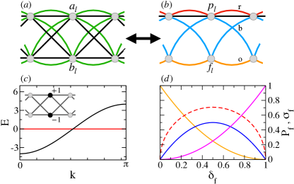
Figure 1: (a) The network (7,8) with $\hat{\mathcal{H}}_{\text{sp}}$ (straight black) and $\hat{\mathcal{H}}_{\text{int}}$ (curved green). (b) Detangled $\hat{\mathcal{H}}$ network with $\hat{\mathcal{H}}_{\text{sp}}$ (straight black), $\hat{\mathcal{H}}_{\text{int}}^{\text{d}}$ [curved red (r)], $\hat{\mathcal{H}}_{\text{int}}^{\text{df}}$ [curved blue (b)] and $\hat{\mathcal{H}}_{\text{int}}^{\text{f}}$ [curved orange (o)]. (c) Band structure of $\hat{\mathcal{H}}_{\text{sp}}$ (7), with the inset indicating the nonzero amplitude locations of an $E=0$ FB CLS (black filled circles). (d) Probabilities $P_{\text{f}}(\varepsilon_{l}=0)$ (orange), $P_{\text{f}}(\varepsilon_{l}=V)$ (blue), $P_{\text{f}}(\varepsilon_{l}=2V)$ (magenta) and standard deviation $\sigma_{\text{f}}$ (red dashed) of $\hat{\varepsilon}_{l}$ in Eq. (10) for $V=1$ versus $\delta_{\text{f}}$.

The local unitary transformation $\hat{a}_{l}=(\hat{p}_{l}+\hat{f}_{l})/\sqrt{2}$ and $\hat{b}_{l}=(\hat{p}_{l}-\hat{f}_{l})/\sqrt{2}$ introduced in Ref. Flach et al., 2014 detangles the Hamiltonian $\hat{\mathcal{H}}_{\text{sp}}$ (7) in $\hat{\mathcal{H}}_{\text{sp}}^{\text{d}}=-2\sum_{l}\bigl{[}\hat{p}_{l}^{\dagger}\hat{p}_{l+1}+\text{h.c.}\bigr{]}$ with $\hat{\mathcal{H}}_{\text{sp}}^{\text{f}}=0$. Moreover, the interaction $\hat{\mathcal{H}}_{\text{int}}$ (8) is invariant under that rotation. In this new basis $\hat{\mathcal{H}}_{\text{int}}$ breaks down into three components $\hat{\mathcal{H}}_{\text{int}}^{\text{f}}=\sum_{l}\hat{n}_{f,l}\hat{n}_{f,l+1}$, $\hat{\mathcal{H}}_{\text{int}}^{\text{d}}=\sum_{l}\hat{n}_{p,l}\hat{n}_{p,l+1}$, and $\hat{\mathcal{H}}_{\text{int}}^{\text{df}}=\sum_{l}\bigl{[}\hat{n}_{p,l}\hat{n}_{f,l+1}+\hat{n}_{f,l}\hat{n}_{p,l+1}\bigr{]}$ which are shown in Fig. 1(b) with orange, red and blue curves respectively.

The Hamiltonian $\hat{\mathcal{H}}^{\{{\bf q}\}}$ (6) and its potential $\hat{\varepsilon}_{l}$ read

$$\hat{\mathcal{H}}^{\{{\bf q}\}} =\sum_{l}\big{[}\hat{\varepsilon}_{l}\hat{n}_{p,l}-2(\hat{p}_{l}^{\dagger}\hat{p}_{l+1}+\text{h.c.})+V\hat{n}_{p,l}\hat{n}_{p,l+1}\big{]}$$ (9)

$$\qquad\hat{\varepsilon}_{l}=V(\hat{q}_{l+1}+\hat{q}_{l-1}),$$ (10)

with $\hat{n}_{p,l}=\hat{p}_{l}^{\dagger}\hat{p}_{l}$. The conserved quantities $\hat{q}_{l}=\hat{f}_{l}^{\dagger}\hat{f}_{l}$ take the values $\{0,1\}$. Hence $\hat{\mathcal{H}}^{\{{\bf q}\}}$ describes interacting spinless fermions in a one-dimensional chain with a random ternary potential $\varepsilon_{l}\in\{0,V,2V\}$. Ternary disorder with equal probabilities $1/3$ has been studied in Ref. Janarek et al., 2018 where an MBL transition was reported for the Heisenberg spin-$1/2$ chain by varying the strength of interaction and disorder independently. Our case is trickier, since both disorder and interaction strengths are tuned by the same control parameter $V$ in Eq. (9). Further, the probabilities of $\varepsilon_{l}=\{0,V,2V\}$ depend on the filling fraction $\delta_{\text{f}}$ of the flatband component: $P_{\text{f}}(\varepsilon_{l}=0)=(1-\delta_{\text{f}})^{2}$, $P_{\text{f}}(\varepsilon_{l}=V)=2\delta_{\text{f}}(1-\delta_{\text{f}})$ and $P_{\text{f}}(\varepsilon_{l}=2V)=\delta_{\text{f}}^{2}$. The curves are shown in Fig. 1(d) including the standard deviation $\sigma_{\text{f}}=V\sqrt{2\delta_{\text{f}}(1-\delta_{\text{f}})}$. The average potential value $\langle\varepsilon_{l}\rangle_{l}=2V\delta_{\text{f}}$. Note as well that equal probabilities $1/3$ are never realized for any filling fraction value.

We identify the transition between ergodic (thermalized, metallic, delocalized) and non-ergodic (non-thermalized, insulating, localized) regimes of our system by computing the energy-resolved adjacent gap ratio $r^{(n)}=\min(s^{(n)},s^{(n+1)})/\max(s^{(n)},s^{(n+1)})$ with $s^{(n)}=E_{n}-E_{n-1}$ for the eigenenergies $E_{n}$ Oganesyan and Huse (2007). The expectation is that the ergodic regime corresponds to the Gaussian Orthogonal Ensemble (GOE) with $r_{\text{GOE}}=0.5307$ Atas et al. (2013). At variance, the non-ergodic regime should yield a Poisson distribution of level spacings with $r_{\text{Poisson}}\approx 0.3863$.

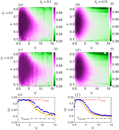
Figure 2: (a-d) Energy resolved mean adjacent gap ratio $\langle r\rangle$ versus $(\epsilon,V)$ for model (9,10). (a) $\delta_{\text{d}}=0.5;\delta_{\text{f}}=0.5$; (b) $\delta_{\text{d}}=0.25;\delta_{\text{f}}=0.5$; (c) $\delta_{\text{d}}=0.5;\delta_{\text{f}}=0.25$; (d) $\delta_{\text{d}}=0.25;\delta_{\text{f}}=0.25$. (e) $\langle r\rangle$ versus $V$ for $\epsilon=0.5$ at $\delta_{\text{f}}=0.5$ (orange) and $\delta_{\text{f}}=0.25$ (blue) for $\delta_{\text{d}}=0.5$. (f) Same as (e) for $\delta_{\text{d}}=0.25$. The system size $L=16$ for all cases.

We diagonalize $\hat{\mathcal{H}}^{\{{\bf q}\}}$ in Eq. (9) for $L=16$ sites with open boundary conditions averaging over $200$ realizations at fixed filling fractions $\delta_{\text{f}}$ and $\delta_{\text{d}}$ – i.e. over 200 sectors of the Hilbert space . Following Ref. Luitz et al. (2015), the spectrum is normalized as $\epsilon(E_{n})=(E_{n}-E_{\text{min}})/(E_{\text{max}}-E_{\text{min}})$ for each realization, divided into $50$ intervals, and the mean adjacent gap ratio $\langle r\rangle$ is computed for each segment separately. The results are reported in Fig. 2 (a-d). In all cases, the MBL transition emerges at large enough interaction strength $V\gg 1$. Note that the MBL transition occurs for different values of $V$ within different irreducible sectors of the Hilbert space characterized by different pairs of filling fractions $(\delta_{\text{f}},\delta_{\text{d}})$ despite sharing the same global filling $\delta$ – e͡.g. Figs. 2 (b,c).

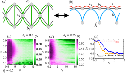
Figure 3: (a) The network (11,12) with $\hat{\mathcal{H}}_{\text{sp}}$ (straight black) and $\hat{\mathcal{H}}_{\text{int}}$ (curved green). (b) Detangled network  (13) with $\hat{\mathcal{H}}_{\text{int}}^{\text{d}}$ [red (r)] and $\hat{\mathcal{H}}_{\text{int}}^{\text{df}}$ [blue (b)]. (c-d) Energy resolved mean adjacent gap ratio $\langle r\rangle$ versus $(\epsilon,V)$ for (c) $\delta_{\text{d}}=0.5;\delta_{\text{f}}=0.5$; (d) $\delta_{\text{d}}=0.25;\delta_{\text{f}}=0.5$. (e) $\langle r\rangle$ versus $V$ around $\epsilon=0.5$ at $\delta_{\text{d}}=0.5$ (blue) and $\delta_{\text{d}}=0.25$ (orange) for $\delta_{\text{f}}=0.25$. The system size $L=16$ for all cases.

Our construction also explains the non-ergodic dynamics observed for a $\nu=3$ case with spinless fermions in Ref. Daumann et al., 2020. The model is shown in Fig. 3(a) and it is described by the Hamiltonian $\hat{\mathcal{H}}=\hat{\mathcal{H}}_{\text{sp}}+V\hat{\mathcal{H}}_{\text{int}}$ with

$$\small\hat{\mathcal{H}}_{\text{sp}} =-\sum_{l}\big{[}(\hat{a}_{l}^{\dagger}+\hat{b}_{l}^{\dagger})(\hat{c}_{l}+\hat{c}_{l+1})+\text{h.c.}\big{]}$$ (11)

$$\hat{\mathcal{H}}_{\text{int}} =\sum_{l}\bigl{[}\hat{n}_{a,l}+\hat{n}_{b,l}\bigr{]}\bigl{[}\hat{n}_{c,l}+\hat{n}_{c,l+1}\bigr{]}+\hat{n}_{a,l}\hat{n}_{b,l}$$ (12)

The single particle spectrum of $\hat{\mathcal{H}}_{\text{sp}}$ consists of two dispersive bands $E_{1,2}({\bf k})=\pm 2\sqrt{2}\cos({\bf k}/2)$ and a flatband $E=0$ with orthonormal CLS. Detangling local unitary transformations for the single particle Hamiltonian have been reported in Ref. Flach et al., 2014. For spinless fermions, the resulting system is shown in Fig. 3(b). In the new basis the product terms in Eq. (12) decompose into $\hat{\mathcal{H}}_{\text{int}}^{\text{f}}=0$, $\hat{\mathcal{H}}_{\text{int}}^{\text{d}}=\sum_{l}\hat{n}_{p,l}(\hat{n}_{c,l}+\hat{n}_{c,l+1})$, and $\hat{\mathcal{H}}_{\text{int}}^{\text{df}}=\sum_{l}\hat{n}_{f,l}(\hat{n}_{c,l}+\hat{n}_{c,l+1})$ – defining the Hamiltonian

$$\hat{\mathcal{H}}^{\{{\bf q}\}} =\sum_{l}\big{[}\hat{\varepsilon}_{l}\hat{n}_{c,l}-\sqrt{2}(\hat{p}_{l}^{\dagger}\hat{c}_{l}+\hat{p}_{l}^{\dagger}\hat{c}_{l+1}+\text{h.c})$$ (13)

$$\qquad+V\hat{n}_{p,l}(\hat{n}_{c,l}+\hat{n}_{c,l+1})\big{]}$$

with the potential $\hat{\varepsilon}_{l}=V(\hat{q}_{l-1}+\hat{q}_{l})$. Interestingly, the terms $\hat{n}_{a,l}\hat{n}_{b,l}$ result in $\hat{p}_{l}^{\dagger}\hat{p}_{l}^{\dagger}\hat{f}_{l}\hat{f}_{l}+\text{h.c}$ in addition to the Hubbard interaction terms on $p,f$ sites which could violate the finetuning. These terms need more than one particle per state and therefore disappear for spinless fermions. Consequently they do not enter $\hat{\mathcal{H}}^{\{{\bf q}\}}$ in Eq. (13). However such terms will appear for e.g. bosons and spinful fermions, and will move pairs of particles between sublattices $\mathcal{F}$ to $\mathcal{D}$. Consequently the quantities $\hat{q}_{l}$ will be no longer conserved for spinful fermions or bosons, and will wash out the irreducible sectors in the Hilbert space of $\hat{\mathcal{H}}$. In Fig. 3 (c-d) we plot the energy-resolved mean adjacent gap ratio $\langle r\rangle$ for two pairs of filling factors $\delta_{\text{d}}$ and $\delta_{\text{f}}$ upon increasing the interaction strength $V$. We observe signatures of an MBL transition for large $V\gg 1$. The transition is further visualized in Fig. 3 (e) where we plot the energy-resolved mean $\langle r\rangle$ versus $V$ around $\epsilon=0.5$.

Conclusions — To conclude, we showed that disorder free many body localization is obtained for flatband networks with finetuned interaction. The flatband supports compact localized states, and the finetuning locks particles in these states even in the presence of interaction. These locked particles turn into scatterers for particles from dispersive states. These families have been obtained by fine-tuning two–body interaction terms on single particle lattices that host dispersive bands and flat bands with orthonormal sets of CLS. We showed that these scatterers are equivalent to conserved quantities and enter the Hamiltonian of the system inducing an effective disorder. We studied numerically two sample cases, Eqs. (7,8) and Eqs. (11,12), for spinless fermions in 1D, confirming that such disorder indeed induces many-body localization transition upon changing the interaction strength. The proposed fine-tuning scheme applies in any lattice dimensions and for any type of many-body statistics. We therefore arrive at a systematic generic generator of quantum many-body systems characterized by an extensive number of local conserved operators, which result in ergodicity breaking phenomena. Another important extension is that we can abandon the translational invariance of $\hat{\mathcal{H}}$ and consider local rotations and/or the energies $E_{a}$ in Eq. (2) unit cell dependent; one can also consider flatband Hamiltonians $\hat{\mathcal{H}}_{\text{sp}}$ without orthonormal sets of CLS Leykam et al. (2017).

Our findings explain recent spinless fermion results for a rhombic lattice considered by Daumann et.al. Daumann et al. (2020); Khare and Choudhury (2020) (orthonormal set of CLS) as well as for a sawtooth ladder considered by Khare et.al. Khare and Choudhury (2020) (non-orthonormal set of CLS). It is straightforward to observe that for total filling fraction $\delta\leq 1/\nu$ there are exact eigenstates with all particles confined to single particle CLS. These eigenstates coexist with extended eigenstates characterized by volume-law entanglement, and become flatband many-body quantum scars Hart et al. (2020b); McClarty et al. (2020); Kuno et al. (2020a); Danieli et al. (2020a). Many-body quantum scars are related to weak ergodicity breaking phenomena Turner et al. (2018); Serbyn et al. (2020); Pilatowsky-Cameo et al. (2021).

The above obtained fine-tuned models can be both appealing from a purely mathematical point of view, and for experimentally relevant setups. Indeed, flatband networks have been indeed experimentally realized in diverse platforms, such as ultra cold atoms Taie et al. (2015) and photonic lattices Mukherjee et al. (2015); Vicencio et al. (2015); Weimann et al. (2016) – see also Derzhko et al. (2015); Leykam et al. (2018); Leykam and Flach (2018). Flatband systems with orthonormal CLS allow the energy levels $E_{\text{FB}}$ in Eq. (2) to be freely tuned. They can thus either cross the dispersive bands $E_{a}(\mathbf{k})$ in Eq. (3) or be gapped away from dispersive bands. This freedom allows to tune the flatband energy at the Fermi level, and to load the particles into the flatband states prior reaching the complete filling of dispersive bands in an experimentally achievable way.

Acknowledgments — This work was supported by the Institute for Basic Science (Project number IBS-R024-D1). We thank I. Khaymovich for helpful discussions.

References

- Anderson (1958) P. W. Anderson, “Absence of diffusion in certain random lattices,” Phys. Rev. 109, 1492–1505 (1958).
- Fleishman and Anderson (1980) L. Fleishman and P. W. Anderson, “Interactions and the anderson transition,” Phys. Rev. B 21, 2366–2377 (1980).
- Altshuler et al. (1997) Boris L. Altshuler, Yuval Gefen, Alex Kamenev, and Leonid S. Levitov, “Quasiparticle lifetime in a finite system: A nonperturbative approach,” Phys. Rev. Lett. 78, 2803–2806 (1997).
- Jacquod and Shepelyansky (1997) Ph. Jacquod and D. L. Shepelyansky, “Emergence of quantum chaos in finite interacting fermi systems,” Phys. Rev. Lett. 79, 1837–1840 (1997).
- Gornyi et al. (2005) I. V. Gornyi, A. D. Mirlin, and D. G. Polyakov, “Interacting electrons in disordered wires: Anderson localization and low- transport,” Phys. Rev. Lett. 95, 206603 (2005).
- Basko et al. (2006) D.M. Basko, I.L. Aleiner, and B.L. Altshuler, “Metal–insulator transition in a weakly interacting many-electron system with localized single-particle states,” Ann. Phys. 321, 1126 – 1205 (2006).
- Abanin and Papić (2017) Dmitry A. Abanin and Zlatko Papić, “Recent progress in many-body localization,” Ann. Phys. 529, 1700169 (2017).
- Abanin et al. (2019) Dmitry A. Abanin, Ehud Altman, Immanuel Bloch, and Maksym Serbyn, “Colloquium: Many-body localization, thermalization, and entanglement,” Rev. Mod. Phys. 91, 021001 (2019).
- Schiulaz et al. (2015) Mauro Schiulaz, Alessandro Silva, and Markus Müller, “Dynamics in many-body localized quantum systems without disorder,” Phys. Rev. B 91, 184202 (2015).
- van Horssen et al. (2015) Merlijn van Horssen, Emanuele Levi, and Juan P. Garrahan, “Dynamics of many-body localization in a translation-invariant quantum glass model,” Phys. Rev. B 92, 100305 (2015).
- Pino et al. (2016) Manuel Pino, Lev B. Ioffe, and Boris L. Altshuler, “Nonergodic metallic and insulating phases of Josephson junction chains,” PNAS 113, 536–541 (2016).
- Hickey et al. (2016) James M Hickey, Sam Genway, and Juan P Garrahan, “Signatures of many-body localisation in a system without disorder and the relation to a glass transition,” J. Stat. Mech.s 2016, 054047 (2016).
- Mondaini and Cai (2017) Rubem Mondaini and Zi Cai, “Many-body self-localization in a translation-invariant hamiltonian,” Phys. Rev. B 96, 035153 (2017).
- Schulz et al. (2019) M. Schulz, C. A. Hooley, R. Moessner, and F. Pollmann, “Stark many-body localization,” Phys. Rev. Lett. 122, 040606 (2019).
- Smith et al. (2017a) A. Smith, J. Knolle, D. L. Kovrizhin, and R. Moessner, “Disorder-free localization,” Phys. Rev. Lett. 118, 266601 (2017a).
- Smith et al. (2017b) A. Smith, J. Knolle, R. Moessner, and D. L. Kovrizhin, “Absence of ergodicity without quenched disorder: From quantum disentangled liquids to many-body localization,” Phys. Rev. Lett. 119, 176601 (2017b).
- Smith et al. (2018) Adam Smith, Johannes Knolle, Roderich Moessner, and Dmitry L. Kovrizhin, “Dynamical localization in lattice gauge theories,” Phys. Rev. B 97, 245137 (2018).
- Brenes et al. (2018) Marlon Brenes, Marcello Dalmonte, Markus Heyl, and Antonello Scardicchio, “Many-body localization dynamics from gauge invariance,” Phys. Rev. Lett. 120, 030601 (2018).
- Karpov et al. (2021) P. Karpov, R. Verdel, Y.-P. Huang, M. Schmitt, and M. Heyl, “Disorder-free localization in an interacting 2d lattice gauge theory,” Phys. Rev. Lett. 126, 130401 (2021).
- Hart et al. (2020a) Oliver Hart, Sarang Gopalakrishnan, and Claudio Castelnovo, “Logarithmic entanglement growth from disorder-free localisation in the two-leg compass ladder,” (2020a), arXiv:2009.00618 [cond-mat.str-el] .
- Sala et al. (2020) Pablo Sala, Tibor Rakovszky, Ruben Verresen, Michael Knap, and Frank Pollmann, “Ergodicity breaking arising from hilbert space fragmentation in dipole-conserving hamiltonians,” Phys. Rev. X 10, 011047 (2020).
- Yang et al. (2020) Zhi-Cheng Yang, Fangli Liu, Alexey V. Gorshkov, and Thomas Iadecola, “Hilbert-space fragmentation from strict confinement,” Phys. Rev. Lett. 124, 207602 (2020).
- Scherg et al. (2020) Sebastian Scherg, Thomas Kohlert, Pablo Sala, Frank Pollmann, Bharath H. M., Immanuel Bloch, and Monika Aidelsburger, “Observing non-ergodicity due to kinetic constraints in tilted fermi-hubbard chains,” (2020), arXiv:2010.12965 [cond-mat.quant-gas] .
- Derzhko et al. (2015) Oleg Derzhko, Johannes Richter, and Mykola Maksymenko, “Strongly correlated flat-band systems: The route from heisenberg spins to hubbard electrons,” Int. J. Mod. Phys. B 29, 1530007 (2015).
- Leykam et al. (2018) Daniel Leykam, Alexei Andreanov, and Sergej Flach, “Artificial flat band systems: from lattice models to experiments,” Adv. Phys.: X 3, 1473052 (2018).
- Leykam and Flach (2018) Daniel Leykam and Sergej Flach, “Perspective: Photonic flatbands,” APL Photonics 3, 070901 (2018).
- Flach et al. (2014) Sergej Flach, Daniel Leykam, Joshua D. Bodyfelt, Peter Matthies, and Anton S. Desyatnikov, “Detangling flat bands into Fano lattices,” Europhys. Lett. 105, 30001 (2014).
- Dias and Gouveia (2015) R. G. Dias and J. D. Gouveia, “Origami rules for the construction of localized eigenstates of the Hubbard model in decorated lattices,” Sci. Rep. 5, 16852 EP – (2015).
- Ramachandran et al. (2017) Ajith Ramachandran, Alexei Andreanov, and Sergej Flach, “Chiral flat bands: Existence, engineering, and stability,” Phys. Rev. B 96, 161104(R) (2017).
- Maimaiti et al. (2017) Wulayimu Maimaiti, Alexei Andreanov, Hee Chul Park, Oleg Gendelman, and Sergej Flach, “Compact localized states and flat-band generators in one dimension,” Phys. Rev. B 95, 115135 (2017).
- Röntgen et al. (2018) M. Röntgen, C. V. Morfonios, and P. Schmelcher, “Compact localized states and flat bands from local symmetry partitioning,” Phys. Rev. B 97, 035161 (2018).
- Toikka and Andreanov (2018) L. A. Toikka and A. Andreanov, “Necessary and sufficient conditions for flat bands in m-dimensional n-band lattices with complex-valued nearest-neighbour hopping,” J Phys. A: Math. Theor 52, 02LT04 (2018).
- Maimaiti et al. (2019) Wulayimu Maimaiti, Sergej Flach, and Alexei Andreanov, “Universal flat band generator from compact localized states,” Phys. Rev. B 99, 125129 (2019).
- Maimaiti et al. (2021) Wulayimu Maimaiti, Alexei Andreanov, and Sergej Flach, “Flat-band generator in two dimensions,” Phys. Rev. B 103, 165116 (2021).
- Tovmasyan et al. (2018) Murad Tovmasyan, Sebastiano Peotta, Long Liang, Päivi Törmä, and Sebastian D. Huber, “Preformed pairs in flat bloch bands,” Phys. Rev. B 98, 134513 (2018).
- Tilleke et al. (2020) Simon Tilleke, Mirko Daumann, and Thomas Dahm, “Nearest neighbour particle-particle interaction in fermionic quasi one-dimensional flat band lattices,” Z. Naturforsch. A 75, 20190371 (2020).
- Danieli et al. (2020a) Carlo Danieli, Alexei Andreanov, Thudiyangal Mithun, and Sergej Flach, “Quantum caging in interacting many-body all-bands-flat lattices,” (2020a), arXiv:2004.11880 [cond-mat.quant-gas] .
- Hart et al. (2020b) Oliver Hart, Giuseppe De Tomasi, and Claudio Castelnovo, “From compact localized states to many-body scars in the random quantum comb,” Phys. Rev. Research 2, 043267 (2020b).
- McClarty et al. (2020) Paul A. McClarty, Masudul Haque, Arnab Sen, and Johannes Richter, “Disorder-free localization and many-body quantum scars from magnetic frustration,” Phys. Rev. B 102, 224303 (2020).
- Kuno et al. (2020a) Yoshihito Kuno, Tomonari Mizoguchi, and Yasuhiro Hatsugai, “Flat band quantum scar,” Phys. Rev. B 102, 241115 (2020a).
- Danieli et al. (2020b) Carlo Danieli, Alexei Andreanov, and Sergej Flach, “Many-body flatband localization,” Phys. Rev. B 102, 041116(R) (2020b).
- Kuno et al. (2020b) Yoshihito Kuno, Takahiro Orito, and Ikuo Ichinose, “Flat-band many-body localization and ergodicity breaking in the Creutz ladder,” New J. Phys. 22, 013032 (2020b).
- Orito et al. (2020) Takahiro Orito, Yoshihito Kuno, and Ikuo Ichinose, “Exact projector hamiltonian, local integrals of motion, and many-body localization with symmetry-protected topological order,” Phys. Rev. B 101, 224308 (2020).
- Roy et al. (2020) Nilanjan Roy, Ajith Ramachandran, and Auditya Sharma, “Interplay of disorder and interactions in a flat-band supporting diamond chain,” Phys. Rev. Research 2, 043395 (2020).
- Daumann et al. (2020) Mirko Daumann, Robin Steinigeweg, and Thomas Dahm, “Many-body localization in translational invariant diamond ladders with flat bands,” (2020), arXiv:2009.09705 [cond-mat.stat-mech] .
- Khare and Choudhury (2020) Rishabh Khare and Sayan Choudhury, “Localized dynamics following a quantum quench in a non-integrable system: an example on the sawtooth ladder,” Journal of Physics B: Atomic, Molecular and Optical Physics 54, 015301 (2020).
- Janarek et al. (2018) Jakub Janarek, Dominique Delande, and Jakub Zakrzewski, “Discrete disorder models for many-body localization,” Phys. Rev. B 97, 155133 (2018).
- Oganesyan and Huse (2007) Vadim Oganesyan and David A. Huse, “Localization of interacting fermions at high temperature,” Phys. Rev. B 75, 155111 (2007).
- Atas et al. (2013) Y. Y. Atas, E. Bogomolny, O. Giraud, and G. Roux, “Distribution of the ratio of consecutive level spacings in random matrix ensembles,” Phys. Rev. Lett. 110, 084101 (2013).
- Note (1) No changes in the mobility edge profiles appeared while averaging over a different number of realizations.
- Luitz et al. (2015) David J. Luitz, Nicolas Laflorencie, and Fabien Alet, “Many-body localization edge in the random-field heisenberg chain,” Phys. Rev. B 91, 081103 (2015).
- Leykam et al. (2017) Daniel Leykam, Joshua D. Bodyfelt, Anton S. Desyatnikov, and Sergej Flach, “Localization of weakly disordered flat band states,” Eur. Phys. J. B 90, 1 (2017).
- Turner et al. (2018) C. J. Turner, A. A. Michailidis, D. A. Abanin, M. Serbyn, and Z. Papic, “Weak ergodicity breaking from quantum many-body scars,” Nat. Phys. 14, 745749 (2018).
- Serbyn et al. (2020) Maksym Serbyn, Dmitry A. Abanin, and Zlatko Papić, “Quantum many-body scars and weak breaking of ergodicity,” (2020), arXiv:2011.09486 [quant-ph] .
- Pilatowsky-Cameo et al. (2021) Saul. Pilatowsky-Cameo, David Villasenor, Miguel A. Bastarrachea-Magnani, Sergio Lerma-Hernandez, Lea F. Santos, and Jorge G. Hirsch, “Ubiquitous quantum scarring does not prevent ergodicity,” Nat. Comm. 12, 852 (2021).
- Taie et al. (2015) Shintaro Taie, Hideki Ozawa, Tomohiro Ichinose, Takuei Nishio, Shuta Nakajima, and Yoshiro Takahashi, “Coherent driving and freezing of bosonic matter wave in an optical Lieb lattice,” Sci. Adv. 1 (2015).
- Mukherjee et al. (2015) Sebabrata Mukherjee, Alexander Spracklen, Debaditya Choudhury, Nathan Goldman, Patrik Öhberg, Erika Andersson, and Robert R. Thomson, “Observation of a localized flat-band state in a photonic Lieb lattice,” Phys. Rev. Lett. 114, 245504 (2015).
- Vicencio et al. (2015) Rodrigo A. Vicencio, Camilo Cantillano, Luis Morales-Inostroza, Bastián Real, Cristian Mejía-Cortés, Steffen Weimann, Alexander Szameit, and Mario I. Molina, “Observation of localized states in Lieb photonic lattices,” Phys. Rev. Lett. 114, 245503 (2015).
- Weimann et al. (2016) Steffen Weimann, Luis Morales-Inostroza, Bastián Real, Camilo Cantillano, Alexander Szameit, and Rodrigo A. Vicencio, “Transport in sawtooth photonic lattices,” Opt. Lett. 41, 2414–2417 (2016).