Enhanced predictive skills in physically-consistent way: Physics Informed Machine Learning for Hydrological Processes
Abstract
Current modeling approaches for hydrological modeling often rely on either physics-based or data-science methods, including Machine Learning (ML) algorithms. While physics-based models tend to rigid structure resulting in unrealistic parameter values in certain instances, ML algorithms establish the input-output relationship while ignoring the constraints imposed by well-known physical processes. While there is a notion that the physics model enables better process understanding and ML algorithms exhibit better predictive skills, scientific knowledge that does not add to predictive ability may be deceptive. Hence, there is a need for hybrid modelling approach to couple ML algorithms and physics-based model in synergistic manner. Here we develop a Physics Informed Machine Learning (PIML) model that combines the process understanding of conceptual hydrological model with predictive abilities of state-of-the-art ML models. We apply the proposed model to predict the monthly time series of the target (streamflow) and intermediate variables (actual evapotranspiration) in the Narmada river basin in India. Our results show the capability of the PIML model to outperform a purely conceptual model ( model) and ML algorithms while ensuring the physical consistency in outputs validated through water balance analysis. The systematic approach for combining conceptual model structure with ML algorithms could be used to improve the predictive accuracy of crucial hydrological processes important for flood risk assessment.
Civil Engineering Discipline, Indian Institute of Technology, Gandhinagar, India Computer Science and Engineering Discipline, Indian Institute of Technology, Gandhinagar, India
Udit Bhatiabhatia.u@iitgn.ac.in
Model to combine predictive ability of machine learning with process understanding of physics-based models for hydrological processes.
Variants of architecture adapted for uncertainty quantification in both target (streamflow) and intermediate variables (evapotranspiration).
Performance gains in prediction of target and intermediate variables; annual water balance analysis reveals physical consistency of model.
1 Introduction
Streamflow prediction, flood protection, and water resource management challenges continue to be highly relevant for societal as well as economic security and well-being [Butts \BOthers. (\APACyear2004), Niu \BBA Feng (\APACyear2021)]. With the ever-increasing availability of computational resources, diverse spatiotemporal datasets from remotely-sensed and in-situ measurements, and advances in Machine Learning (ML) algorithms, data-driven approaches are being used widely to predict the response of catchments to meteorological forcings, including precipitation and surface temperature [Tongal \BBA Booij (\APACyear2018), Parisouj \BOthers. (\APACyear2020), Feng \BOthers. (\APACyear2020)]. Despite recent advances in their predictive performance and ability to handle highly complex spatiotemporal datasets, the success of ML algorithms in the domain applications remains elusive due to limited interpretability [Gilpin \BOthers. (\APACyear2018)], physical inconsistencies and persistent issues of equifinality (different model structures and parameterization schemes giving the same end state with equal accuracy) [Schmidt \BOthers. (\APACyear2020), Beven (\APACyear2006)]. To address interpretability challenges, physics-based models, which encapsulate our domain knowledge and physics principles, including conservation of mass, energy, and momentum through mathematical equations, remain the tool of choice for researchers and practitioners [Vieux \BOthers. (\APACyear2004), Beven (\APACyear1989)]. Physics-based models are broadly categorized as conceptual models and physically-based models. These models involve mathematical and semi-empirical equations with the physical basis [Devia \BOthers. (\APACyear2015)]. In addition to meteorological and hydrological observations, these models’ predictive performance critically relies on identifying the right set of parameters, which is typically achieved through the process of calibration [Fenicia \BOthers. (\APACyear2007)]. While there is a notion that physics-based models enable better process understanding, and ML methods lead to better predictive skills, the process understanding that does not add to predictive ability may be specious, and improved predictive skills devoid of physical realism may not generalize to unexpected, yet possible scenarios [Ganguly \BOthers. (\APACyear2014)]. With the growing realization that neither purely ML algorithms nor physics-based models suffice to address the domain-specific challenges, physics guided machine learning approaches are gaining significant attention in scientific and engineering domains, aiming to integrate the data and scientific knowledge in a complementary manner [Muralidhar \BOthers. (\APACyear2019), Wang \BOthers. (\APACyear2017), Zhang \BOthers. (\APACyear2020)].
Multiple frameworks, both conceptual and applied, for combining physics with machine learning approaches have been proposed in the literature for diverse applications. For example, \citeAwagner2016theory have demonstrated the importance of scientific reasoning for discovering reliable structure, property, and processing models, as well as listed nuances associated with machine learning applications in material science. \citeAwang2017physics have proposed a data-driven, physics-informed machine learning (PIML) approach for reconstructing discrepancies in Reynolds-averaged Navier Stokes modeled Reynolds stresses. It is achieved by training existing direct numerical simulation databases through machine learning techniques and applied the PIML approach for different flow conditions such as turbulent flows developed in the square duct for varying Reynolds numbers and flows with massive separation. \citeAmuralidhar2019physics have demonstrated the application of physics-guided model architecture for predicting drag force acting on each particle in fluid flow. Further, they have incorporated physics-based loss functions to capture physical knowledge, avoid constraint violation, and develop a physics-guided deep neural network model. For seismic response modeling, \citeAzhang2020physics have developed a physics-guided convolutional network architecture to predict a building’s seismic response. \citeAfaghmous2014theory, \citeAreichstein2019deep, and \citeAganguly2014toward have highlighted the need to have scalable data science methods which can incorporate physical and conceptual understanding for better interpretation for applications in earth and atmospheric sciences. The authors themselves noted that while there exist multiple opportunities in the area of incorporating contextual cues from the domain into machine learning models, the domain-specific challenges (that is, preservation of spatiotemporal structures, confidence and uncertainty representation in predictions) should be accounted for to ensure physical consistency in the outputs.
karpatne2017physics and \citeAjia2019physics developed physics-guided variants of ML models that guide neural network architectures to simulate lake temperature profiles in a physically consistent manner. Specifically, \citeAkarpatne2017physics demonstrated how to combine the standard neural network models with the energy conservation laws to outperform purely knowledge-based or data-driven models. These goals were achieved in two ways. First, the outputs from physics-based models were fed into ML architecture. Secondly, they introduced physical knowledge-based constraints in the temporal ML model’s objective function (Long Short Term Memory (LSTM) in this case). \citeAliang2019physics generated a database through simulations of the physics-based model and then processed it with different data-driven approaches to predict the quantity and quality of surface water in agricultural fields. Recently, \citeAlu2021streamflow introduced a physics-informed LSTM model to improve the prediction when data is out of distribution. The physics-based Precipitation Runoff Modeling System (PRMS) model-simulated streamflow and meteorological features were given as inputs to the LSTM for the streamflow prediction. We argue that while these approaches could help to improve the predictive abilities of purely physics-driven or ML models, the gains in terms of interpretability and capability of these hybrid models to capture the intermediate variables realistically are yet to be explored. \citeAkhandelwal2020physics has proposed the LSTM based architecture for streamflow prediction, which emulates the Soil and Water Assessment Tool (SWAT), a physically-based semi-distributed model. They used the same inputs as the SWAT model into three LSTMs in the first layer to simulate soil water, evapotranspiration, and snowpack. The outputs obtained from the first layer were combined with the original SWAT inputs to feed into another LSTM to model the streamflow. We note that this is one of a few physics-guided data sciences approaches for hydrological modeling that accounts for intermediate variables (i.e., soil water, evapotranspiration, and snowpack). However, a typical SWAT architecture involves multiple intermediate fluxes (e.g., evapotranspiration, surface runoff, groundwater flow, percolation, lateral flow, groundwater recharge, deep aquifer recharge) and state variables (e.g., soil water, snowpack, deep aquifer storage, shallow aquifer storage) [Neitsch \BOthers. (\APACyear2004)], which were altogether ignored in their architecture, hence limiting the interpretability of outputs.
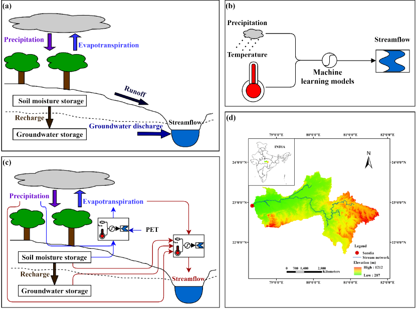
In this study, we design a modeling framework to combine the conceptual hydrological model with state-of-the-art ML models to leverage ML algorithms’ predictive ability with process understanding of physics-based models in a synergistic manner. Specifically, we use the structure of the abcd model to identify the input (precipitation, potential evapotranspiration, groundwater storage, and soil moisture), intermediate (actual evapotranspiration), and target variables (streamflow at particular gauge location) at various steps (Figure 1c). Then, we replace empirical equations of our conceptual model (the model) with ML algorithms at various steps to identify the relationships between input and output (both intermediate and target) variables. Our model design is inspired by the fact that conceptual hydrological models involve empirical and semi-empirical equations, which are generally developed and validated for specific basins. Therefore, their application outside the basin boundaries calls for abundant caution. We argue that the use of ML algorithms to identify the complex relationships between input and output variables at various stages of the modeling process adds flexibility to the models having rigid mathematical structures. Hence, PIML models can generalize to the basins where empirical equations of conceptual models may not generalize. We demonstrate the PIML models’ ability to capture the intermediate variables with greater accuracy, which in turn transpire into better model performance to model target variable (streamflow in the present case) compared to conceptual and pure data-driven architectures. Finally, we demonstrate the ability of variants of the PIML models to capture the water balance effectively. We demonstrate the proposed model’s applicability on the Narmada River Basin with gauge station at Sandia (Figure 1d). We use a suite of Machine Learning and Deep Learning architectures commonly used in numerous hydrological and earth sciences applications, including LSTMs [Kratzert \BOthers. (\APACyear2018)], Least absolute shrinkage and selection operator (LASSO) and Ridge Regression [Yu \BBA Liong (\APACyear2007), Lange \BBA Sippel (\APACyear2020)], Support Vector Regression [Deka \BOthers. (\APACyear2014)], Gaussian Process Regression [Sun \BOthers. (\APACyear2014)], and Bayesian LSTMs [Lu \BOthers. (\APACyear2021)] for purely ML-based as well as hybrid PIML models.
We organize the rest of the manuscript as follows: in section 2, we present the brief overview of the conceptual model and ML algorithms used in this study. Details of the proposed PIML model and various evaluation metrics deployed in this study are also discussed. In section 3, we discuss the details of the study area and datasets used in this research. In section 4, we compare physics-based, ML, and PIDS algorithms using metrics discussed in section 2. Finally, we discuss the physical consistency of PIML models by performing a water-balance analysis.
2 Methods
This section presents the review of the conceptual abcd model and various ML models with underlying equations used in this study. Further, we discuss the architecture of the PIML model. Finally, we present a brief overview of various performance metrics used throughout this study.
2.1 Review of the model
The model is a simple Water Balance (WB) conceptual hydrological model proposed by \citeAthomas1981improved. While it was originally developed to examine the catchment scale water balances at annual scales, variants of the model have been applied for regional and local hydrological investigations at monthly scales [Alley (\APACyear1984), Vandewiele \BOthers. (\APACyear1992)]. The conceptual model involves the parsimonious yet adequate description of various hydrological processes at catchment scale with the lesser computational cost making it highly popular in operational and research practice [Clark \BBA Kavetski (\APACyear2010)]. Specifically, the model structure has been widely used for hypotheses testing, model performance evaluation [Martinez \BBA Gupta (\APACyear2010), Bai \BOthers. (\APACyear2015)], and hydrological uncertainty reduction experiments [W. Li \BBA Sankarasubramanian (\APACyear2012)] owing to a highly realistic representation of various hydrological processes despite its simple structure. Figure 1a shows the conceptual representation of the model. The model consists of two storage compartments: soil moisture stoarage and groundwater storage. Inputs required are monthly precipitation and potential evapotranspiration , while output generated is streamflow . This model is calibrated with four parameters, , , , and . The parameter , controls the amount of direct runoff when soil is unsaturated, and parameter reflects the upper bound of the total of actual evapotranspiration and soil moisture at a given time step. The groundwater recharge is controlled by parameter , while parameter , decides the amount of groundwater storage to be converted to groundwater discharge . The direct runoff and groundwater discharge together generate the streamflow. The model includes two state variables: (available water) and . While is the sum of precipitation at a given time step and soil moisture at the previous time step, represents the sum of actual evapotranspiration and soil moisture at a given time step. Equations 1a-1b show the mass balance for soil moisture and groundwater storage compartments. Equations 1d-1e are typical examples of parameterized relationships among various variables (See Supplementary Information (SI) for complete set of equations).
| (1a) | |||
| (1b) | |||
| (1c) | |||
| (1d) | |||
| (1e) |
2.2 Review of Machine Learning Algorithms
Recent advances in the field of machine learning have provided many methodological opportunities to meet the evolving needs and challenges of hydrological research. ML models have demonstrated superior performance in learning patterns and generalizations as well as extracting patterns from complex streams of geospatial and hydrological datasets [Lange \BBA Sippel (\APACyear2020), Reichstein \BOthers. (\APACyear2019)]. ML algorithms form the core of the proposed PIML model. Hence, a review of various methods used in this study is presented to clarify the subsequent sections.
Long Short Term Memory (LSTM) is an artificial neural network architecture that has gained popularity for sequential data problems. In the context of hydrology, LSTMs have been used for rainfall-runoff modeling at hourly [Xiang \BOthers. (\APACyear2020)], daily [Fu \BOthers. (\APACyear2020), Cheng \BOthers. (\APACyear2020)], monthly [Cheng \BOthers. (\APACyear2020)] time steps as well as for the improvement in the predictions of the physics-based models [T. Yang \BOthers. (\APACyear2019)]. LSTMs are a special kind of recurrent neural networks (RNNs) capable of learning long-term temporal dependencies. The simple RNNs have an issue of vanishing gradient, which can be removed by LSTMs with the introduction of gates and memory cells [Hochreiter \BBA Schmidhuber (\APACyear1997)].
Bayesian Neural Networks (BNNs) have advantages over neural networks, such as they can handle small data well while generating uncertainty bounds of predictions. Since BNNs incorporate posterior inference in standard neural networks, these architectures have gained popularity for uncertainty quantification [Marshall \BOthers. (\APACyear2004), J. Yang \BOthers. (\APACyear2007), Raje \BBA Krishnan (\APACyear2012)]. Recently \citeAlu2021streamflow has applied Bayesian LSTM for uncertainty quantification in streamflow prediction. BNNs were made by approximating the intractable Bayesian Inference. BayesByBackprop [Blundell \BOthers. (\APACyear2015)] is a backpropagation-compatible algorithm to learn probability distribution of a neural network. The same concept is extended to create Bayesian LSTM. BNNs can provide us uncertainty on weights by sampling them from a distribution parameterized by trainable variables [Esposito (\APACyear2020)].
Gaussian Process Regression (GPR) is a non-parametric kernel-based probabilistic model, which has gained wider popularity in the domain of ML [Williams \BBA Rasmussen (\APACyear2006)]. Unlike various ML algorithms that determine the exact values of parameters, GPR infers the probability distribution over all possible values using the prior distribution and updated distribution (known as a posterior distribution) that incorporates information from both prior distribution and available data. Researchers have used the GPR for daily [Rasouli \BOthers. (\APACyear2012)] and monthly [Sun \BOthers. (\APACyear2014)] streamflow forecasting.
Support Vector Machine (SVM) is developed for classification, and it is extended to regression by \citeAvapnik1995nature. Support Vector Regression (SVR) is one the most popular ML approaches used for daily [Dibike \BOthers. (\APACyear2001), Malik \BOthers. (\APACyear2020)] and monthly [Maity \BOthers. (\APACyear2010)] streamflow predictions. SVRs can efficiently learn the non-linear relationships between predictors (input variables) and predictands (output variables) using the kernel trick, which maps the inputs into linearly solvable high-dimensional feature spaces.
The least absolute shrinkage and selection operator (LASSO) [Tibshirani (\APACyear1996)], and Ridge Regression [Hoerl \BBA Kennard (\APACyear1970)] are some of the simplest techniques which are widely used to reduce model complexity and prevent overfitting. LASSO regression works by reducing the model complexity and feature selection by penalizing the absolute sum of coefficients. As a result of this regularization, some of the coefficients that do not affect the output are reduced to zero. In Ridge regression, the square of the coefficients’ magnitude is penalized instead of the absolute sum. When coefficients take large values, the objective function (typically Mean Square Error function) is penalized, resulting in the coefficients’ shrinking during the optimization process. LASSO and Ridge regressions have been widely applied for streamflow forecasting, and their outputs have been found comparable with state-of-the-art ML algorithms [Lima \BBA Lall (\APACyear2010), Chokmani \BOthers. (\APACyear2008), Xiang \BOthers. (\APACyear2020)].
The details of all the ML models used in this study are presented in SI.
2.3 Physics Informed Machine Learning model
The proposed PIML model provides a way to combine the physics-based conceptual model with various ML approaches to enable better process understanding and improve predictive performance while being mindful of physical consistencies (e.g., water balance). The proposed model’s premise is as follows: use the covariate structure of the physics-based conceptual model (the model in this case) and replace rigid mathematical relationships among input and output variables at various steps using ML algorithms. While the conceptual model structure provides the physics-informed choice of covariates and interpretable structure, ML algorithms help in extracting complex relationships between the input and output variables. For example, in the model, is non-linear function of , , and (Equations 1c, 1d and 1e). In the PIML model, we use , , and as inputs (or predictors) into our embedded ML model and obtain the estimate of using various ML algorithms (deployed independently) described in Figure 1c. The estimates of thus obtained is combined with , , , and to obtain new covariate matrix, which is then fed into next layer of ML algorithm to obtain the final estimates of (target variable in this case). We note that choice of these covariates is governed by the water-balance equation (Equation 2a):
In general form, the functional relationship for the and can be written as follows.
| (2a) | |||
| (2b) |
The exact function form of and is determined by embedded ML models (Figure 1c).
2.4 Evaluation metrics
For model performance evaluation, we have used Nash-Sutcliffe Efficiency (NSE), Percent Bias (PBIAS), Root Mean Square Error (RMSE). Widely used in various hydrological applications [Najafi \BBA Moradkhani (\APACyear2016), Swain \BBA Patra (\APACyear2017), Paul \BOthers. (\APACyear2019), Wagena \BOthers. (\APACyear2020)], these metrics assess model efficiency, biases in the model predictions, and estimate errors in the model outputs, respectively.
2.4.1 Nash-Sutcliffe Efficiency
The NSE [Nash \BBA Sutcliffe (\APACyear1970)] is a reliable and widely used statistic to assess goodness of fit for hydrological models [McCuen \BOthers. (\APACyear2006)]. The NSE value has a range of to 1.0. When the NSE value is 1, it shows a perfect match between modeled output and observed data, while if it is less than 0, it shows observed mean is a better predictor than the model output. Following equation shows the formula for NSE calculation:
| (3a) | |||
| where, , , and are model output, observed data, and mean of observed data, respectively. | |||
2.4.2 Percent Bias
It helps to determine how well the model can estimate the average magnitudes of the required output. The PBIAS ranges from to . Its optimal value is 0, while the positive and negative values show model underpredicts and overpredicts, respectively.
| (3b) |
2.4.3 Root Mean Square Error
It is the measure of deviations in model output from observed data. The RMSE ranges from 0 to , and when it is equal to 0, it shows both modeled output and observed data are perfectly match each other.
| (3c) |
The model performance is evaluated using the criteria outlined in \citeAmoriasi2015hydrologic. For monthly simulation, , , and, , the model performance is considered as very good, good, satisfactory and unsatisfactory, respectively. Negative NSE values indicates the model performance is unacceptable.
3 Study area and datasets
To illustrate the proposed model’s applicability, we have selected the part of the Narmada river basin up to gauge station located at Sandia (Figure 1d). Flowing through the states of Gujarat and Madhya Pradesh, the Narmada River is a 1312 km long river draining a 98796 area. The study area considered here has a drainage area of 38,571 . The daily precipitation and (minimum and maximum) temperature at and spatial resolution, respectively, are obtained from the India Meteorological Department (IMD) for the period of 1979 – 2014. The observed streamflow data of the Sandia gauge station (22.92°N, 78.35°E) is obtained from the India Water Resources Information System (India-WRIS; https://indiawris.gov.in/). The daily soil moisture, groundwater storage, and evapotranspiration are obtained from Global Land Data Assimilation System (GLDAS) Catchment Land Surface Model L4 daily datasets, available through the archives of the Goddard Earth Sciences Data and Information Services Center (GES DISC) of National Aeronautics and Space Administration (NASA) .
| Data | Spatial resolution | Source |
|---|---|---|
| Precipitation | 0.25° | IMD [Pai \BOthers. (\APACyear2014)] |
| Minimum and maximum temperature | 1° | IMD [Srivastava \BOthers. (\APACyear2009)] |
| Soil moisture, groundwater storage and actual evapotranspiration | 0.25° | GLDAS [B. Li \BOthers. (\APACyear2019)] |
| Streamflow | Gauge at Sandia | India-WRIS |
We calculate the potential evapotranspiration using the Hargreaves method (equation 4) [Hargreaves \BBA Samani (\APACyear1985)]. The daily PET values are summed up to monthly values, followed by spatial averaging over the study region.
| (4) |
where, PET is potential evapotranspiration in mm/day and is the extra-terrestrial radiation in . , and, are maximum, minimum and average surface temperature in degree Celsius respectively.
To assess the algorithm’s generalizability, we consider distinct training and testing periods while ensuring that the test set does not contain examples from the training sets. Specifically, we use the window of 1979-2008 for training and 2009-2014 for validating the models on testing data. We kept similar training and testing data for the model, ML models, and the PIML model. The additional warm-up period required for the model is selected as 1976-1978. Subsequently, all evaluation metrics (See Results) are calculated on the test set.
4 Results
4.1 Evaluating performance of the physics-based model
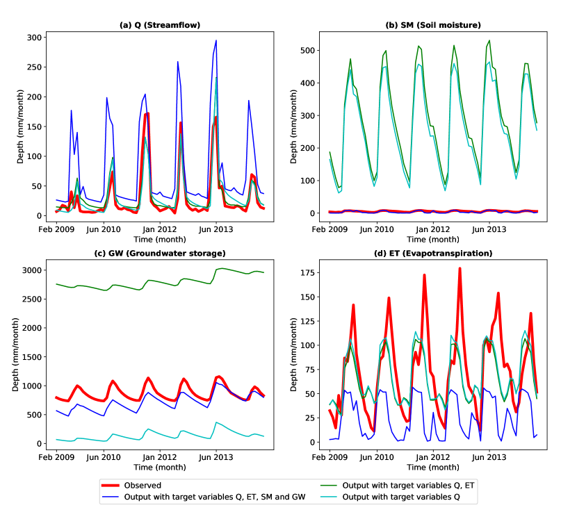
Here, we evaluate the performance of the model in predicting target and intermediate variables. We have considered the three cases. In each case, we use the same model structure but calibrate: (a) modeled streamflow (Q) against observed Q; (b) modeled Q and ET against observed Q and ET, respectively; and (c) modeled Q, SM, GW, and ET against observed Q, SM, GW, and ET, respectively. For all these cases, we use particle swarm optimization to estimate the parameters. The model warm-up and calibration period are selected as 1976-1978 and 1979-2008, respectively. We test the calibrated model’s performance for all cases using monthly data from 2009-2014 (same as the period of testing data used in all ML algorithms throughout the study). Results for all three cases are shown in Figure 2. Table 2 summarizes the calibrated model’s performance in terms of key performance metrics for the three cases. The model performance is evaluated using the criteria outlined in \citeAmoriasi2015hydrologic. For cases (a) and (b), model performance is categorized as ”very good.” In contrast, for case(c), the performance is classified as unacceptable in modeling the streamflow (based on the values of NSE). However, in case (b), despite calibrating the model for both Q and ET, the predictive performance on intermediate variable (ET) remains ”unacceptable.” Further, for case (c), we observe that the model performance was ”unacceptable” for all the predicted variables, including streamflow. Our results imply that while it is possible to obtain remarkable performances on target variables through the calibration process, even simple conceptual models may not simulate various intermediate processes consistently, which are otherwise important for interpretability (as observed in case (a)). The results thus obtained underscore the need to seriously consider model structure, generalizability, and intermediate process representations in physics-based models [Kirchner (\APACyear2006)].
| Variable | ET | Q | ||||
| Performance metric | RMSE | PBIAS | NSE | RMSE | PBIAS | NSE |
| (a) Target: Q | 30.443 | -6.495 | 0.438 | 17.767 | 8.392 | 0.815 |
| (b) Target: Q and ET | 31.519 | -10.381 | 0.397 | 17.172 | 11.296 | 0.827 |
| (c) Target: Q, ET, SM and GW | 60.860 | -65.289 | -1.247 | 64.303 | 145.771 | -1.423 |
| Variable | SM | GW | ||||
| Performance metric | RMSE | PBIAS | NSE | RMSE | PBIAS | NSE |
| (a) Target: Q | 286.336 | 4862.764 | -23967.799 | 739.475 | -84.398 | -37.014 |
| (b) Target: Q and ET | 314.685 | 5384.296 | -28948.883 | 1934.970 | 221.640 | -259.286 |
| (c) Target: Q, ET, SM and GW | 2.776 | -35.066 | -1.253 | 180.558 | -17.592 | -1.266 |
4.2 Performance evaluation of ML Algorithms
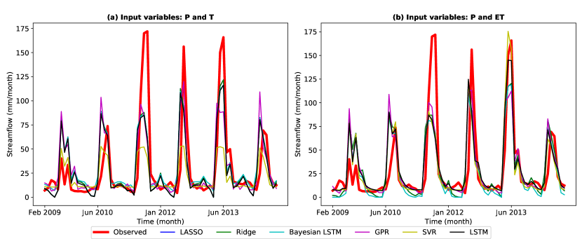
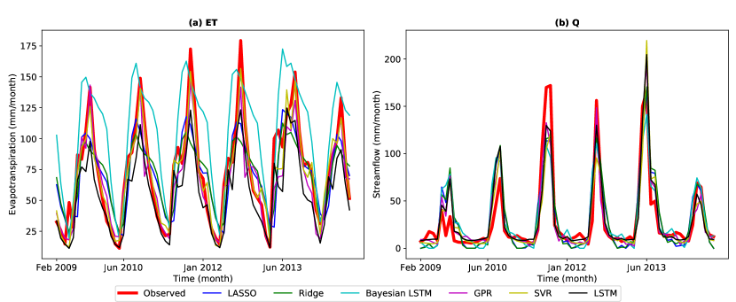
Before we discuss the results of the PIML model, we present the performance of various ML algorithms to model streamflow with a different set of input variables. These ML algorithms would be embedded into the structure of the conceptual model. Thus, it is imperative to understand the ability of ML models to capture relatively straightforward rainfall-runoff relationships. Specifically, we use (a) inputs as precipitation and average temperature and (b) inputs as precipitation and actual evapotranspiration. Figure 3a and 3b shows the comparison of all the ML models with observed streamflow for both cases. Performance metrics for all the algorithms are summarized in Table 3.
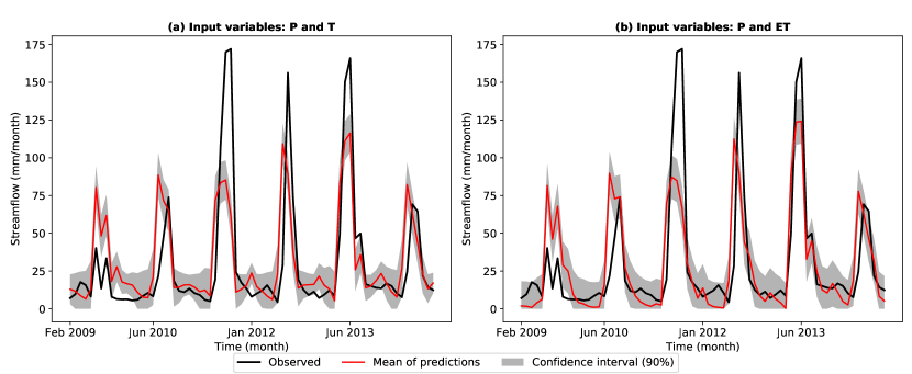
For case (a), LSTM, LASSO, Ridge, Bayesian LSTM exhibit satisfactory performance, whereas performance SVR and GPR lie in the ”unsatisfactory” range. Similarly, for case (b), we note that all the models’ performance is in the ”satisfactory” range based on the NSE criteria. Though Bayesian LSTM shows higher PBIAS, the improved NSE and decreased RMSE highlight the improvements in the model prediction, which can be attributed to input variables’ choice. Further, we adapt the architecture of Bayesian LSTMs to quantify the associated epistemic uncertainty (Fig. 4). We note that despite various ML models’ ability to capture the non-linear relationship between predictors and predictands and their scalability, it is often difficult for users to comprehend why specific predictions are made. Thus, there is an opportunity to combine ML and Physics-Based models’ architectures in a complementary way to address the associated limitations. In this study, we achieve this by using the model structure and embed ML algorithms in the proposed PIML model to simulate intermediate processes.
| Input variables | (a) P and T | (b) P and ET | ||||
|---|---|---|---|---|---|---|
| Performance metric | RMSE | PBIAS | NSE | RMSE | PBIAS | NSE |
| LSTM | 28.104 | -6.721 | 0.537 | 27.252 | 4.322 | 0.565 |
| LASSO | 28.037 | -2.624 | 0.539 | 27.899 | -0.312 | 0.544 |
| Ridge | 28.041 | -2.638 | 0.539 | 27.902 | -0.307 | 0.544 |
| SVR | 33.420 | -31.625 | 0.346 | 27.098 | -1.003 | 0.570 |
| GPR | 30.008 | -2.056 | 0.472 | 27.600 | 1.107 | 0.554 |
| Bayesian LSTM | 28.198 | 5.684 | 0.534 | 27.730 | -15.230 | 0.549 |
4.3 Performance Evaluation of PIML model
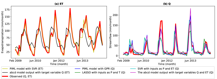
We evaluate the performance of the PIML model for an intermediate variable (Actual ET) and streamflow (Q) for which credible observations are available for both training and testing periods(Figure 5a and 5b). Table 4 summarizes the results of the PIML models embedded with various ML algorithms. The NSE value for Q shows that PIML models embedded with LSTM and GPR perform ”very good” while other models exhibit ”good” performance. We compare the performance of the PIML approach with the corresponding ML approach. For example, the performance of the model embedded with GPR and purely ML-based GPR algorithm are compared. We note consistent improvement in the NSE values obtained from monthly Q for all 6 cases of PIML (Table 4) compared to ML algorithms’ performance (Table 3). Further, we note that the best performing PIML architectures (+GPR, and +LSTM) even outperform the model (Table 2). Further, we calculate the model performance on predicting ET and note that 2 (PIML+SVR), (PIML+GPR) out of 6 variants of PIML exhibit ”very good” performance, whereas three variants (PIML+LASSO, PIML+Ridge, PIML+LSTM) can be classified as satisfactory. These five models also outperform the model in predicting monthly ET, thus highlighting the superiority of PIML models in predicting target and intermediate variables.
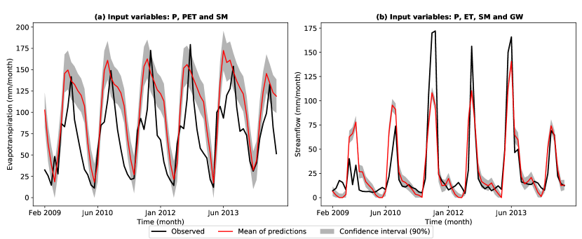
Further, we demonstrate how PIML approaches can be tailored to quantify uncertainties in the predictions of intermediate and target variables. Specifically, we quantify the uncertainties in modeled ET and Q using + Bayesian LSTM variant of PIML. Predictions of Q and ET with 90 percent confidence interval are shown in Figure 6a and Figure 6b, respectively, for the testing period. In addition to the superior performance of the PIML model, we also notice the reduction in uncertainty bounds in predictions of Q compared to purely ML-based algorithms (Figure 4b).
As noted earlier, in addition to improved prediction accuracy over pure physics or ML-based approaches, PIML approaches should generate outputs consistent with physical laws such as conservation of mass. In the context of hydrology, it is imperative to assess the model’s ability to simulate annual water balance realistically.
To check annual water balance, the sum of precipitation should be equal to actual ET, streamflow, and change in soil moisture and groundwater storage. For our study area, soil moisture and groundwater storage changes are observed as -0.045 mm and -0.155 mm, respectively. As these values are negligible in comparison to other terms in the water balance equation, the changes in storage are thus ignored [Szilagyi (\APACyear2020)].
Here, we consider three variants of PIML: (a) PIML with SVR; (b)PIML with GPR; and (c) PIML with SVR and GPR. While PIML with GPR performs the best in predicting Q, PIML with SVR outperformed other variants in predicting ET. Hence, we experiment with the hybrid variant: SVR for modeling ET in the first layer and GPR to model Q in the second layer in our PIML architecture. It is noteworthy that P, ET, and Q are obtained from three sources (Table LABEL:table:1). Therefore, an initial difference of -9.884 mm is observed between P and the sum of ET and Q. We calculate the percentage deviation in ET+Q for all the variants, with observations taken as a benchmark. Variant (c) exhibits deviation of -1.893 , whereas variants (a) and (b) have the deviation of -3.255 , -6.754 respectively in annual water balance (Table 5). The lower values of deviation for three cases demonstrate the ability of PIML approaches to simulate annual water balance consistently.
| Variable | ET | Q | ||||
|---|---|---|---|---|---|---|
| Performance metric | RMSE | PBIAS | NSE | RMSE | PBIAS | NSE |
| LSTM | 22.704 | -23.966 | 0.687 | 16.083 | 4.124 | 0.848 |
| LASSO | 25.975 | -3.303 | 0.591 | 20.901 | 3.796 | 0.744 |
| Ridge | 27.023 | -4.013 | 0.557 | 21.02 | 4.259 | 0.741 |
| SVR | 11.703 | -2.543 | 0.917 | 19.719 | -4.975 | 0.772 |
| GPR | 16.407 | -9.287 | 0.837 | 15.001 | -0.626 | 0.868 |
| Bayesian LSTM | 41.819 | 41.635 | -0.061 | 21.242 | 2.572 | 0.736 |
| Model/observed | P | ET | Q | ET + Q | Percentage of deviation |
|---|---|---|---|---|---|
| Observed | 1231.783 | 878.549 | 363.118 | 1241.667 | 0 |
| PIML with SVR | 1231.783 | 856.204 | 345.053 | 1201.257 | -3.255 |
| PIML with GPR | 1231.783 | 796.954 | 360.847 | 1157.801 | -6.754 |
| PIML with SVR and GPR | 1231.783 | 856.204 | 361.962 | 1218.166 | -1.893 |
5 Conclusion
Physics-guided and physics-informed data science approaches have received significant attention in the recent past [Muralidhar \BOthers. (\APACyear2019), Wang \BOthers. (\APACyear2017), Zhang \BOthers. (\APACyear2020), Karpatne \BOthers. (\APACyear2017)]. Several architectures in disparate fields have been proposed to improve the predictive abilities of pure physics-based and ML approaches in a physically consistent manner. Hydrological modeling is a non-linear and complex problem with ample scope for improvement. In this study, we propose the PIML model for predicting target as well as intermediate variables. We demonstrate the applicability of this model on a single hydrological unit to predict monthly time-series of actual evapotranspiration and streamflow, the two key variables in hydrological processes [Xiong \BOthers. (\APACyear2019)].
The proposed PIML model is the first-of-its-kind to provide an intuitive way to combine physically interpretable architectures of lumped hydrological models with state-of-the-art ML algorithms in a meaningful way. We also study the ability of these models to quantify uncertainties in both intermediate and target variables. For our study area, outputs from the PIML model exhibited high prediction performance compared to pure physics-based or ML approaches. Besides, we observe a significant reduction in the uncertainty bounds for predictions of both variables. We also assessed the ability of the PIML models to simulate the annual water budget and noted consistent performance for various variants.
The PIML model presented in this manuscript allows us to capture complex and non-linear dependencies between hydrological variables while being mindful of the logical sequence which the physics-based model guides. The proposed approach provides a way to add flexibility to otherwise rigid model structures of state-of-the-art hydrological models widely used in hydrology. While we demonstrate the applicability of this approach using a simple WB model ( model), this approach can be extended to other conceptual models, which may involve a much larger number of intermediate steps.
Future extensions to the PIML framework for hydrological applications need to be validated for distributed as well as semi-distributed model structures, as well as for daily and sub-daily time-steps. Moreover, we have ignored the role of upstream reservoirs, which might impact the predictive skills of models, especially at daily and sub-daily scales. Also, the performance of the PIML model is highly sensitive to the choice of ML algorithms used at various intermediate steps. As of now, there are no proven guidelines on the best ML model selection. Despite these outlined limitations, the application of the proposed framework can be extended to various scientific and engineering problems such as early warning systems, risk and reliability assessment for hydraulic structures, and flood management.
Acknowledgements.
Funding for the project is provided by Scheme for Transformational and Advances in Sciences of Ministry of Education implemented by Indian Institute of Science, Bangalore (Research Project ID: 367 titled ’Physics Guided Data Science Approach for Predictive Understanding of Hydrological Processes’). The authors thank Professor Auroop Ganguly from Northeastern University, Boston for helpful discussions, and IIT Gandhinagar colleagues Professor Nipun Batra, and Divya Upadhyay for comments on the manuscript.References
- Alley (\APACyear1984) \APACinsertmetastaralley1984treatment{APACrefauthors}Alley, W\BPBIM. \APACrefYearMonthDay1984. \BBOQ\APACrefatitleOn the treatment of evapotranspiration, soil moisture accounting, and aquifer recharge in monthly water balance models On the treatment of evapotranspiration, soil moisture accounting, and aquifer recharge in monthly water balance models.\BBCQ \APACjournalVolNumPagesWater Resources Research2081137–1149. \PrintBackRefs\CurrentBib
- Bai \BOthers. (\APACyear2015) \APACinsertmetastarbai2015comparison{APACrefauthors}Bai, P., Liu, X., Liang, K.\BCBL \BBA Liu, C. \APACrefYearMonthDay2015. \BBOQ\APACrefatitleComparison of performance of twelve monthly water balance models in different climatic catchments of China Comparison of performance of twelve monthly water balance models in different climatic catchments of china.\BBCQ \APACjournalVolNumPagesJournal of Hydrology5291030–1040. \PrintBackRefs\CurrentBib
- Beven (\APACyear1989) \APACinsertmetastarbeven1989changing{APACrefauthors}Beven, K. \APACrefYearMonthDay1989. \BBOQ\APACrefatitleChanging ideas in hydrology—the case of physically-based models Changing ideas in hydrology—the case of physically-based models.\BBCQ \APACjournalVolNumPagesJournal of hydrology1051-2157–172. \PrintBackRefs\CurrentBib
- Beven (\APACyear2006) \APACinsertmetastarbeven2006manifesto{APACrefauthors}Beven, K. \APACrefYearMonthDay2006. \BBOQ\APACrefatitleA manifesto for the equifinality thesis A manifesto for the equifinality thesis.\BBCQ \APACjournalVolNumPagesJournal of hydrology3201-218–36. \PrintBackRefs\CurrentBib
- Blundell \BOthers. (\APACyear2015) \APACinsertmetastarpmlr-v37-blundell15{APACrefauthors}Blundell, C., Cornebise, J., Kavukcuoglu, K.\BCBL \BBA Wierstra, D. \APACrefYearMonthDay201507–09 Jul. \BBOQ\APACrefatitleWeight Uncertainty in Neural Network Weight uncertainty in neural network.\BBCQ \BIn F. Bach \BBA D. Blei (\BEDS), \APACrefbtitleProceedings of the 32nd International Conference on Machine Learning Proceedings of the 32nd international conference on machine learning (\BVOL 37, \BPGS 1613–1622). \APACaddressPublisherLille, FrancePMLR. {APACrefURL} http://proceedings.mlr.press/v37/blundell15.html \PrintBackRefs\CurrentBib
- Butts \BOthers. (\APACyear2004) \APACinsertmetastarbutts2004evaluation{APACrefauthors}Butts, M\BPBIB., Payne, J\BPBIT., Kristensen, M.\BCBL \BBA Madsen, H. \APACrefYearMonthDay2004. \BBOQ\APACrefatitleAn evaluation of the impact of model structure on hydrological modelling uncertainty for streamflow simulation An evaluation of the impact of model structure on hydrological modelling uncertainty for streamflow simulation.\BBCQ \APACjournalVolNumPagesJournal of hydrology2981-4242–266. \PrintBackRefs\CurrentBib
- Cheng \BOthers. (\APACyear2020) \APACinsertmetastarcheng2020long{APACrefauthors}Cheng, M., Fang, F., Kinouchi, T., Navon, I.\BCBL \BBA Pain, C. \APACrefYearMonthDay2020. \BBOQ\APACrefatitleLong lead-time daily and monthly streamflow forecasting using machine learning methods Long lead-time daily and monthly streamflow forecasting using machine learning methods.\BBCQ \APACjournalVolNumPagesJournal of Hydrology590125376. \PrintBackRefs\CurrentBib
- Chokmani \BOthers. (\APACyear2008) \APACinsertmetastarchokmani2008comparison{APACrefauthors}Chokmani, K., Ouarda, T\BPBIB., Hamilton, S., Ghedira, M\BPBIH.\BCBL \BBA Gingras, H. \APACrefYearMonthDay2008. \BBOQ\APACrefatitleComparison of ice-affected streamflow estimates computed using artificial neural networks and multiple regression techniques Comparison of ice-affected streamflow estimates computed using artificial neural networks and multiple regression techniques.\BBCQ \APACjournalVolNumPagesJournal of Hydrology3493-4383–396. \PrintBackRefs\CurrentBib
- Clark \BBA Kavetski (\APACyear2010) \APACinsertmetastarclark2010ancient{APACrefauthors}Clark, M\BPBIP.\BCBT \BBA Kavetski, D. \APACrefYearMonthDay2010. \BBOQ\APACrefatitleAncient numerical daemons of conceptual hydrological modeling: 1. Fidelity and efficiency of time stepping schemes Ancient numerical daemons of conceptual hydrological modeling: 1. fidelity and efficiency of time stepping schemes.\BBCQ \APACjournalVolNumPagesWater Resources Research4610. \PrintBackRefs\CurrentBib
- Deka \BOthers. (\APACyear2014) \APACinsertmetastardeka2014support{APACrefauthors}Deka, P\BPBIC.\BCBT \BOthersPeriod. \APACrefYearMonthDay2014. \BBOQ\APACrefatitleSupport vector machine applications in the field of hydrology: a review Support vector machine applications in the field of hydrology: a review.\BBCQ \APACjournalVolNumPagesApplied soft computing19372–386. \PrintBackRefs\CurrentBib
- Devia \BOthers. (\APACyear2015) \APACinsertmetastardevia2015review{APACrefauthors}Devia, G\BPBIK., Ganasri, B\BPBIP.\BCBL \BBA Dwarakish, G\BPBIS. \APACrefYearMonthDay2015. \BBOQ\APACrefatitleA review on hydrological models A review on hydrological models.\BBCQ \APACjournalVolNumPagesAquatic Procedia41001–1007. \PrintBackRefs\CurrentBib
- Dibike \BOthers. (\APACyear2001) \APACinsertmetastardibike2001model{APACrefauthors}Dibike, Y\BPBIB., Velickov, S., Solomatine, D.\BCBL \BBA Abbott, M\BPBIB. \APACrefYearMonthDay2001. \BBOQ\APACrefatitleModel induction with support vector machines: introduction and applications Model induction with support vector machines: introduction and applications.\BBCQ \APACjournalVolNumPagesJournal of Computing in Civil Engineering153208–216. \PrintBackRefs\CurrentBib
- Esposito (\APACyear2020) \APACinsertmetastaresposito2020blitzbdl{APACrefauthors}Esposito, P. \APACrefYearMonthDay2020. \APACrefbtitleBLiTZ - Bayesian Layers in Torch Zoo (a Bayesian Deep Learing library for Torch). Blitz - bayesian layers in torch zoo (a bayesian deep learing library for torch). \APAChowpublishedhttps://github.com/piEsposito/blitz-bayesian-deep-learning/. \APACaddressPublisherGitHub. \PrintBackRefs\CurrentBib
- Faghmous \BOthers. (\APACyear2014) \APACinsertmetastarfaghmous2014theory{APACrefauthors}Faghmous, J\BPBIH., Banerjee, A., Shekhar, S., Steinbach, M., Kumar, V., Ganguly, A\BPBIR.\BCBL \BBA Samatova, N. \APACrefYearMonthDay2014. \BBOQ\APACrefatitleTheory-guided data science for climate change Theory-guided data science for climate change.\BBCQ \APACjournalVolNumPagesComputer471174–78. \PrintBackRefs\CurrentBib
- Feng \BOthers. (\APACyear2020) \APACinsertmetastarfeng2020enhancing{APACrefauthors}Feng, D., Fang, K.\BCBL \BBA Shen, C. \APACrefYearMonthDay2020. \BBOQ\APACrefatitleEnhancing streamflow forecast and extracting insights using long-short term memory networks with data integration at continental scales Enhancing streamflow forecast and extracting insights using long-short term memory networks with data integration at continental scales.\BBCQ \APACjournalVolNumPagesWater Resources Research569e2019WR026793. \PrintBackRefs\CurrentBib
- Fenicia \BOthers. (\APACyear2007) \APACinsertmetastarfenicia2007comparison{APACrefauthors}Fenicia, F., Savenije, H\BPBIH., Matgen, P.\BCBL \BBA Pfister, L. \APACrefYearMonthDay2007. \BBOQ\APACrefatitleA comparison of alternative multiobjective calibration strategies for hydrological modeling A comparison of alternative multiobjective calibration strategies for hydrological modeling.\BBCQ \APACjournalVolNumPagesWater Resources Research433. \PrintBackRefs\CurrentBib
- Fu \BOthers. (\APACyear2020) \APACinsertmetastarfu2020deep{APACrefauthors}Fu, M., Fan, T., Ding, Z., Salih, S\BPBIQ., Al-Ansari, N.\BCBL \BBA Yaseen, Z\BPBIM. \APACrefYearMonthDay2020. \BBOQ\APACrefatitleDeep learning data-intelligence model based on adjusted forecasting window scale: application in daily streamflow simulation Deep learning data-intelligence model based on adjusted forecasting window scale: application in daily streamflow simulation.\BBCQ \APACjournalVolNumPagesIEEE Access832632–32651. \PrintBackRefs\CurrentBib
- Ganguly \BOthers. (\APACyear2014) \APACinsertmetastarganguly2014toward{APACrefauthors}Ganguly, A\BPBIR., Kodra, E\BPBIA., Agrawal, A., Banerjee, A., Boriah, S., Chatterjee, S.\BDBLWuebbles, D. \APACrefYearMonthDay2014. \BBOQ\APACrefatitleToward enhanced understanding and projections of climate extremes using physics-guided data mining techniques Toward enhanced understanding and projections of climate extremes using physics-guided data mining techniques.\BBCQ \APACjournalVolNumPagesNonlinear Processes in Geophysics214777–795. {APACrefURL} https://npg.copernicus.org/articles/21/777/2014/ {APACrefDOI} 10.5194/npg-21-777-2014 \PrintBackRefs\CurrentBib
- Gilpin \BOthers. (\APACyear2018) \APACinsertmetastargilpin2018explaining{APACrefauthors}Gilpin, L\BPBIH., Bau, D., Yuan, B\BPBIZ., Bajwa, A., Specter, M.\BCBL \BBA Kagal, L. \APACrefYearMonthDay2018. \BBOQ\APACrefatitleExplaining explanations: An overview of interpretability of machine learning Explaining explanations: An overview of interpretability of machine learning.\BBCQ \BIn \APACrefbtitle2018 IEEE 5th International Conference on data science and advanced analytics (DSAA) 2018 ieee 5th international conference on data science and advanced analytics (dsaa) (\BPGS 80–89). \PrintBackRefs\CurrentBib
- Hargreaves \BBA Samani (\APACyear1985) \APACinsertmetastarhargreaves1985reference{APACrefauthors}Hargreaves, G\BPBIH.\BCBT \BBA Samani, Z\BPBIA. \APACrefYearMonthDay1985. \BBOQ\APACrefatitleReference crop evapotranspiration from temperature Reference crop evapotranspiration from temperature.\BBCQ \APACjournalVolNumPagesApplied engineering in agriculture1296–99. \PrintBackRefs\CurrentBib
- Hochreiter \BBA Schmidhuber (\APACyear1997) \APACinsertmetastarhochreiter1997long{APACrefauthors}Hochreiter, S.\BCBT \BBA Schmidhuber, J. \APACrefYearMonthDay1997. \BBOQ\APACrefatitleLong short-term memory Long short-term memory.\BBCQ \APACjournalVolNumPagesNeural computation981735–1780. \PrintBackRefs\CurrentBib
- Hoerl \BBA Kennard (\APACyear1970) \APACinsertmetastarhoerl1970Ridge{APACrefauthors}Hoerl, A\BPBIE.\BCBT \BBA Kennard, R\BPBIW. \APACrefYearMonthDay1970. \BBOQ\APACrefatitleRidge regression: Biased estimation for nonorthogonal problems Ridge regression: Biased estimation for nonorthogonal problems.\BBCQ \APACjournalVolNumPagesTechnometrics12155–67. \PrintBackRefs\CurrentBib
- Jia \BOthers. (\APACyear2019) \APACinsertmetastarjia2019physics{APACrefauthors}Jia, X., Willard, J., Karpatne, A., Read, J., Zwart, J., Steinbach, M.\BCBL \BBA Kumar, V. \APACrefYearMonthDay2019. \BBOQ\APACrefatitlePhysics guided RNNs for modeling dynamical systems: A case study in simulating lake temperature profiles Physics guided rnns for modeling dynamical systems: A case study in simulating lake temperature profiles.\BBCQ \BIn \APACrefbtitleProceedings of the 2019 SIAM International Conference on Data Mining Proceedings of the 2019 siam international conference on data mining (\BPGS 558–566). \PrintBackRefs\CurrentBib
- Karpatne \BOthers. (\APACyear2017) \APACinsertmetastarkarpatne2017physics{APACrefauthors}Karpatne, A., Watkins, W., Read, J.\BCBL \BBA Kumar, V. \APACrefYearMonthDay2017. \BBOQ\APACrefatitlePhysics-guided neural networks (pgnn): An application in lake temperature modeling Physics-guided neural networks (pgnn): An application in lake temperature modeling.\BBCQ \APACjournalVolNumPagesarXiv preprint arXiv:1710.11431. \PrintBackRefs\CurrentBib
- Khandelwal \BOthers. (\APACyear2020) \APACinsertmetastarkhandelwal2020physics{APACrefauthors}Khandelwal, A., Xu, S., Li, X., Jia, X., Stienbach, M., Duffy, C.\BDBLKumar, V. \APACrefYearMonthDay2020. \BBOQ\APACrefatitlePhysics Guided Machine Learning Methods for Hydrology Physics guided machine learning methods for hydrology.\BBCQ \APACjournalVolNumPagesarXiv preprint arXiv:2012.02854. \PrintBackRefs\CurrentBib
- Kirchner (\APACyear2006) \APACinsertmetastarkirchner2006getting{APACrefauthors}Kirchner, J\BPBIW. \APACrefYearMonthDay2006. \BBOQ\APACrefatitleGetting the right answers for the right reasons: Linking measurements, analyses, and models to advance the science of hydrology Getting the right answers for the right reasons: Linking measurements, analyses, and models to advance the science of hydrology.\BBCQ \APACjournalVolNumPagesWater Resources Research423. \PrintBackRefs\CurrentBib
- Kratzert \BOthers. (\APACyear2018) \APACinsertmetastarkratzert2018rainfall{APACrefauthors}Kratzert, F., Klotz, D., Brenner, C., Schulz, K.\BCBL \BBA Herrnegger, M. \APACrefYearMonthDay2018. \BBOQ\APACrefatitleRainfall–runoff modelling using long short-term memory (LSTM) networks Rainfall–runoff modelling using long short-term memory (lstm) networks.\BBCQ \APACjournalVolNumPagesHydrology and Earth System Sciences22116005–6022. \PrintBackRefs\CurrentBib
- Lange \BBA Sippel (\APACyear2020) \APACinsertmetastarlange2020machine{APACrefauthors}Lange, H.\BCBT \BBA Sippel, S. \APACrefYearMonthDay2020. \BBOQ\APACrefatitleMachine learning applications in hydrology Machine learning applications in hydrology.\BBCQ \BIn \APACrefbtitleForest-Water Interactions Forest-water interactions (\BPGS 233–257). \APACaddressPublisherSpringer. \PrintBackRefs\CurrentBib
- B. Li \BOthers. (\APACyear2019) \APACinsertmetastarli2019long{APACrefauthors}Li, B., Rodell, M., Sheffield, J., Wood, E.\BCBL \BBA Sutanudjaja, E. \APACrefYearMonthDay2019. \BBOQ\APACrefatitleLong-term, non-anthropogenic groundwater storage changes simulated by three global-scale hydrological models Long-term, non-anthropogenic groundwater storage changes simulated by three global-scale hydrological models.\BBCQ \APACjournalVolNumPagesScientific reports911–13. \PrintBackRefs\CurrentBib
- W. Li \BBA Sankarasubramanian (\APACyear2012) \APACinsertmetastarli2012reducing{APACrefauthors}Li, W.\BCBT \BBA Sankarasubramanian, A. \APACrefYearMonthDay2012. \BBOQ\APACrefatitleReducing hydrologic model uncertainty in monthly streamflow predictions using multimodel combination Reducing hydrologic model uncertainty in monthly streamflow predictions using multimodel combination.\BBCQ \APACjournalVolNumPagesWater Resources Research4812. \PrintBackRefs\CurrentBib
- Liang \BOthers. (\APACyear2019) \APACinsertmetastarliang2019physics{APACrefauthors}Liang, J., Li, W., Bradford, S\BPBIA.\BCBL \BBA Simunek, J. \APACrefYearMonthDay2019. \BBOQ\APACrefatitlePhysics-Informed Data-Driven Models to Predict Surface Runoff Water Quantity and Quality in Agricultural Fields Physics-informed data-driven models to predict surface runoff water quantity and quality in agricultural fields.\BBCQ \APACjournalVolNumPagesWater112200. \PrintBackRefs\CurrentBib
- Lima \BBA Lall (\APACyear2010) \APACinsertmetastarlima2010climate{APACrefauthors}Lima, C\BPBIH.\BCBT \BBA Lall, U. \APACrefYearMonthDay2010. \BBOQ\APACrefatitleClimate informed monthly streamflow forecasts for the Brazilian hydropower network using a periodic ridge regression model Climate informed monthly streamflow forecasts for the brazilian hydropower network using a periodic ridge regression model.\BBCQ \APACjournalVolNumPagesJournal of hydrology3803-4438–449. \PrintBackRefs\CurrentBib
- Lu \BOthers. (\APACyear2021) \APACinsertmetastarlu2021streamflow{APACrefauthors}Lu, D., Konapala, G., Painter, S\BPBIL., Kao, S\BHBIC.\BCBL \BBA Gangrade, S. \APACrefYearMonthDay2021. \BBOQ\APACrefatitleStreamflow simulation in data-scarce basins using Bayesian and physics-informed machine learning models Streamflow simulation in data-scarce basins using bayesian and physics-informed machine learning models.\BBCQ \APACjournalVolNumPagesJournal of Hydrometeorology. \PrintBackRefs\CurrentBib
- Maity \BOthers. (\APACyear2010) \APACinsertmetastarmaity2010potential{APACrefauthors}Maity, R., Bhagwat, P\BPBIP.\BCBL \BBA Bhatnagar, A. \APACrefYearMonthDay2010. \BBOQ\APACrefatitlePotential of support vector regression for prediction of monthly streamflow using endogenous property Potential of support vector regression for prediction of monthly streamflow using endogenous property.\BBCQ \APACjournalVolNumPagesHydrological Processes: An International Journal247917–923. \PrintBackRefs\CurrentBib
- Malik \BOthers. (\APACyear2020) \APACinsertmetastarmalik2020support{APACrefauthors}Malik, A., Tikhamarine, Y., Souag-Gamane, D., Kisi, O.\BCBL \BBA Pham, Q\BPBIB. \APACrefYearMonthDay2020. \BBOQ\APACrefatitleSupport vector regression optimized by meta-heuristic algorithms for daily streamflow prediction Support vector regression optimized by meta-heuristic algorithms for daily streamflow prediction.\BBCQ \APACjournalVolNumPagesStochastic Environmental Research and Risk Assessment34111755–1773. \PrintBackRefs\CurrentBib
- Marshall \BOthers. (\APACyear2004) \APACinsertmetastarmarshall2004comparative{APACrefauthors}Marshall, L., Nott, D.\BCBL \BBA Sharma, A. \APACrefYearMonthDay2004. \BBOQ\APACrefatitleA comparative study of Markov chain Monte Carlo methods for conceptual rainfall-runoff modeling A comparative study of markov chain monte carlo methods for conceptual rainfall-runoff modeling.\BBCQ \APACjournalVolNumPagesWater Resources Research402. \PrintBackRefs\CurrentBib
- Martinez \BBA Gupta (\APACyear2010) \APACinsertmetastarmartinez2010toward{APACrefauthors}Martinez, G\BPBIF.\BCBT \BBA Gupta, H\BPBIV. \APACrefYearMonthDay2010. \BBOQ\APACrefatitleToward improved identification of hydrological models: A diagnostic evaluation of the “abcd” monthly water balance model for the conterminous United States Toward improved identification of hydrological models: A diagnostic evaluation of the “abcd” monthly water balance model for the conterminous united states.\BBCQ \APACjournalVolNumPagesWater Resources Research468. \PrintBackRefs\CurrentBib
- McCuen \BOthers. (\APACyear2006) \APACinsertmetastarmccuen2006evaluation{APACrefauthors}McCuen, R\BPBIH., Knight, Z.\BCBL \BBA Cutter, A\BPBIG. \APACrefYearMonthDay2006. \BBOQ\APACrefatitleEvaluation of the Nash–Sutcliffe efficiency index Evaluation of the nash–sutcliffe efficiency index.\BBCQ \APACjournalVolNumPagesJournal of hydrologic engineering116597–602. \PrintBackRefs\CurrentBib
- Moriasi \BOthers. (\APACyear2015) \APACinsertmetastarmoriasi2015hydrologic{APACrefauthors}Moriasi, D\BPBIN., Gitau, M\BPBIW., Pai, N.\BCBL \BBA Daggupati, P. \APACrefYearMonthDay2015. \BBOQ\APACrefatitleHydrologic and water quality models: Performance measures and evaluation criteria Hydrologic and water quality models: Performance measures and evaluation criteria.\BBCQ \APACjournalVolNumPagesTransactions of the ASABE5861763–1785. \PrintBackRefs\CurrentBib
- Muralidhar \BOthers. (\APACyear2019) \APACinsertmetastarmuralidhar2019physics{APACrefauthors}Muralidhar, N., Bu, J., Cao, Z., He, L., Ramakrishnan, N., Tafti, D.\BCBL \BBA Karpatne, A. \APACrefYearMonthDay2019. \BBOQ\APACrefatitlePhysics-guided design and learning of neural networks for predicting drag force on particle suspensions in moving fluids Physics-guided design and learning of neural networks for predicting drag force on particle suspensions in moving fluids.\BBCQ \APACjournalVolNumPagesarXiv preprint arXiv:1911.04240. \PrintBackRefs\CurrentBib
- Najafi \BBA Moradkhani (\APACyear2016) \APACinsertmetastarnajafi2016ensemble{APACrefauthors}Najafi, M\BPBIR.\BCBT \BBA Moradkhani, H. \APACrefYearMonthDay2016. \BBOQ\APACrefatitleEnsemble combination of seasonal streamflow forecasts Ensemble combination of seasonal streamflow forecasts.\BBCQ \APACjournalVolNumPagesJournal of Hydrologic Engineering21104015043. \PrintBackRefs\CurrentBib
- Nash \BBA Sutcliffe (\APACyear1970) \APACinsertmetastarnash1970river{APACrefauthors}Nash, J\BPBIE.\BCBT \BBA Sutcliffe, J\BPBIV. \APACrefYearMonthDay1970. \BBOQ\APACrefatitleRiver flow forecasting through conceptual models part I—A discussion of principles River flow forecasting through conceptual models part i—a discussion of principles.\BBCQ \APACjournalVolNumPagesJournal of hydrology103282–290. \PrintBackRefs\CurrentBib
- Neitsch \BOthers. (\APACyear2004) \APACinsertmetastarneitsch2004soil{APACrefauthors}Neitsch, S., Arnold, J., Kiniry, J., Srinivasan, R.\BCBL \BBA Williams, J. \APACrefYearMonthDay2004. \BBOQ\APACrefatitleSoil and water assessment tool input/output file documentation, version 2005: Temple, TX Soil and water assessment tool input/output file documentation, version 2005: Temple, tx.\BBCQ \APACjournalVolNumPagesUS Department of Agriculture, Agricultural Research Service, Grassland, Soil and Water Research Laboratory, available online at:” ftp://ftp. brc. tamus. edu. pub/outgoing/sammons/swat2005” (accessed 11/28/06). \PrintBackRefs\CurrentBib
- Niu \BBA Feng (\APACyear2021) \APACinsertmetastarniu2021evaluating{APACrefauthors}Niu, W\BHBIj.\BCBT \BBA Feng, Z\BHBIk. \APACrefYearMonthDay2021. \BBOQ\APACrefatitleEvaluating the performances of several artificial intelligence methods in forecasting daily streamflow time series for sustainable water resources management Evaluating the performances of several artificial intelligence methods in forecasting daily streamflow time series for sustainable water resources management.\BBCQ \APACjournalVolNumPagesSustainable Cities and Society64102562. \PrintBackRefs\CurrentBib
- Pai \BOthers. (\APACyear2014) \APACinsertmetastarpai2014development{APACrefauthors}Pai, D., Sridhar, L., Rajeevan, M., Sreejith, O., Satbhai, N.\BCBL \BBA Mukhopadhyay, B. \APACrefYearMonthDay2014. \BBOQ\APACrefatitleDevelopment of a new high spatial resolution (0.25 0.25) long period (1901–2010) daily gridded rainfall data set over India and its comparison with existing data sets over the region Development of a new high spatial resolution (0.25 0.25) long period (1901–2010) daily gridded rainfall data set over india and its comparison with existing data sets over the region.\BBCQ \APACjournalVolNumPagesMausam6511–18. \PrintBackRefs\CurrentBib
- Parisouj \BOthers. (\APACyear2020) \APACinsertmetastarparisouj2020employing{APACrefauthors}Parisouj, P., Mohebzadeh, H.\BCBL \BBA Lee, T. \APACrefYearMonthDay2020. \BBOQ\APACrefatitleEmploying machine learning algorithms for streamflow prediction: a case study of four river basins with different climatic zones in the United States Employing machine learning algorithms for streamflow prediction: a case study of four river basins with different climatic zones in the united states.\BBCQ \APACjournalVolNumPagesWater Resources Management34134113–4131. \PrintBackRefs\CurrentBib
- Paul \BOthers. (\APACyear2019) \APACinsertmetastarpaul2019diagnosing{APACrefauthors}Paul, P\BPBIK., Gaur, S., Kumari, B., Panigrahy, N., Mishra, A.\BCBL \BBA Singh, R. \APACrefYearMonthDay2019. \BBOQ\APACrefatitleDiagnosing credibility of a large-scale conceptual hydrological model in simulating streamflow Diagnosing credibility of a large-scale conceptual hydrological model in simulating streamflow.\BBCQ \APACjournalVolNumPagesJournal of Hydrologic Engineering24404019004. \PrintBackRefs\CurrentBib
- Raje \BBA Krishnan (\APACyear2012) \APACinsertmetastarraje2012bayesian{APACrefauthors}Raje, D.\BCBT \BBA Krishnan, R. \APACrefYearMonthDay2012. \BBOQ\APACrefatitleBayesian parameter uncertainty modeling in a macroscale hydrologic model and its impact on Indian river basin hydrology under climate change Bayesian parameter uncertainty modeling in a macroscale hydrologic model and its impact on indian river basin hydrology under climate change.\BBCQ \APACjournalVolNumPagesWater Resources Research488. \PrintBackRefs\CurrentBib
- Rasouli \BOthers. (\APACyear2012) \APACinsertmetastarrasouli2012daily{APACrefauthors}Rasouli, K., Hsieh, W\BPBIW.\BCBL \BBA Cannon, A\BPBIJ. \APACrefYearMonthDay2012. \BBOQ\APACrefatitleDaily streamflow forecasting by machine learning methods with weather and climate inputs Daily streamflow forecasting by machine learning methods with weather and climate inputs.\BBCQ \APACjournalVolNumPagesJournal of Hydrology414284–293. \PrintBackRefs\CurrentBib
- Reichstein \BOthers. (\APACyear2019) \APACinsertmetastarreichstein2019deep{APACrefauthors}Reichstein, M., Camps-Valls, G., Stevens, B., Jung, M., Denzler, J., Carvalhais, N.\BCBL \BBA Prabhat. \APACrefYearMonthDay2019. \BBOQ\APACrefatitleDeep learning and process understanding for data-driven Earth system science Deep learning and process understanding for data-driven earth system science.\BBCQ \APACjournalVolNumPagesNature5667743195–204. \PrintBackRefs\CurrentBib
- Schmidt \BOthers. (\APACyear2020) \APACinsertmetastarschmidt2020challenges{APACrefauthors}Schmidt, L., Heße, F., Attinger, S.\BCBL \BBA Kumar, R. \APACrefYearMonthDay2020. \BBOQ\APACrefatitleChallenges in applying machine learning models for hydrological inference: A case study for flooding events across Germany Challenges in applying machine learning models for hydrological inference: A case study for flooding events across germany.\BBCQ \APACjournalVolNumPagesWater Resources Research565. \PrintBackRefs\CurrentBib
- Srivastava \BOthers. (\APACyear2009) \APACinsertmetastarsrivastava2009development{APACrefauthors}Srivastava, A., Rajeevan, M.\BCBL \BBA Kshirsagar, S. \APACrefYearMonthDay2009. \BBOQ\APACrefatitleDevelopment of a high resolution daily gridded temperature data set (1969–2005) for the Indian region Development of a high resolution daily gridded temperature data set (1969–2005) for the indian region.\BBCQ \APACjournalVolNumPagesAtmospheric Science Letters104249–254. \PrintBackRefs\CurrentBib
- Sun \BOthers. (\APACyear2014) \APACinsertmetastarsun2014monthly{APACrefauthors}Sun, A\BPBIY., Wang, D.\BCBL \BBA Xu, X. \APACrefYearMonthDay2014. \BBOQ\APACrefatitleMonthly streamflow forecasting using Gaussian process regression Monthly streamflow forecasting using gaussian process regression.\BBCQ \APACjournalVolNumPagesJournal of Hydrology51172–81. \PrintBackRefs\CurrentBib
- Swain \BBA Patra (\APACyear2017) \APACinsertmetastarswain2017streamflow{APACrefauthors}Swain, J\BPBIB.\BCBT \BBA Patra, K\BPBIC. \APACrefYearMonthDay2017. \BBOQ\APACrefatitleStreamflow estimation in ungauged catchments using regionalization techniques Streamflow estimation in ungauged catchments using regionalization techniques.\BBCQ \APACjournalVolNumPagesJournal of Hydrology554420–433. \PrintBackRefs\CurrentBib
- Szilagyi (\APACyear2020) \APACinsertmetastarszilagyi2020water{APACrefauthors}Szilagyi, J. \APACrefYearMonthDay2020. \BBOQ\APACrefatitleWater Balance Backward: Estimation of Annual Watershed Precipitation and Its Long-Term Trend with the Help of the Calibration-Free Generalized Complementary Relationship of Evaporation Water balance backward: Estimation of annual watershed precipitation and its long-term trend with the help of the calibration-free generalized complementary relationship of evaporation.\BBCQ \APACjournalVolNumPagesWater1261775. \PrintBackRefs\CurrentBib
- Thomas (\APACyear1981) \APACinsertmetastarthomas1981improved{APACrefauthors}Thomas, H. \APACrefYearMonthDay1981. \BBOQ\APACrefatitleImproved methods for national water assessment Improved methods for national water assessment.\BBCQ \APACjournalVolNumPagesReport WR15249270, US Water Resource Council, Washington, DC. \PrintBackRefs\CurrentBib
- Tibshirani (\APACyear1996) \APACinsertmetastartibshirani1996regression{APACrefauthors}Tibshirani, R. \APACrefYearMonthDay1996. \BBOQ\APACrefatitleRegression shrinkage and selection via the lasso Regression shrinkage and selection via the lasso.\BBCQ \APACjournalVolNumPagesJournal of the Royal Statistical Society: Series B (Methodological)581267–288. \PrintBackRefs\CurrentBib
- Tongal \BBA Booij (\APACyear2018) \APACinsertmetastartongal2018simulation{APACrefauthors}Tongal, H.\BCBT \BBA Booij, M\BPBIJ. \APACrefYearMonthDay2018. \BBOQ\APACrefatitleSimulation and forecasting of streamflows using machine learning models coupled with base flow separation Simulation and forecasting of streamflows using machine learning models coupled with base flow separation.\BBCQ \APACjournalVolNumPagesJournal of hydrology564266–282. \PrintBackRefs\CurrentBib
- Vandewiele \BOthers. (\APACyear1992) \APACinsertmetastarvandewiele1992methodology{APACrefauthors}Vandewiele, G., Xu, C\BHBIY.\BCBL \BOthersPeriod. \APACrefYearMonthDay1992. \BBOQ\APACrefatitleMethodology and comparative study of monthly water balance models in Belgium, China and Burma Methodology and comparative study of monthly water balance models in belgium, china and burma.\BBCQ \APACjournalVolNumPagesJournal of Hydrology1341-4315–347. \PrintBackRefs\CurrentBib
- Vapnik (\APACyear1995) \APACinsertmetastarvapnik1995nature{APACrefauthors}Vapnik, V\BPBIN. \APACrefYearMonthDay1995. \APACrefbtitleThe nature of statistical learning theory. The nature of statistical learning theory. \APACaddressPublisherSpringer-Verlag. \PrintBackRefs\CurrentBib
- Vieux \BOthers. (\APACyear2004) \APACinsertmetastarvieux2004evaluation{APACrefauthors}Vieux, B\BPBIE., Cui, Z.\BCBL \BBA Gaur, A. \APACrefYearMonthDay2004. \BBOQ\APACrefatitleEvaluation of a physics-based distributed hydrologic model for flood forecasting Evaluation of a physics-based distributed hydrologic model for flood forecasting.\BBCQ \APACjournalVolNumPagesJournal of hydrology2981-4155–177. \PrintBackRefs\CurrentBib
- Wagena \BOthers. (\APACyear2020) \APACinsertmetastarwagena2020comparison{APACrefauthors}Wagena, M\BPBIB., Goering, D., Collick, A\BPBIS., Bock, E., Fuka, D\BPBIR., Buda, A.\BCBL \BBA Easton, Z\BPBIM. \APACrefYearMonthDay2020. \BBOQ\APACrefatitleComparison of short-term streamflow forecasting using stochastic time series, neural networks, process-based, and Bayesian models Comparison of short-term streamflow forecasting using stochastic time series, neural networks, process-based, and bayesian models.\BBCQ \APACjournalVolNumPagesEnvironmental Modelling & Software126104669. \PrintBackRefs\CurrentBib
- Wagner \BBA Rondinelli (\APACyear2016) \APACinsertmetastarwagner2016theory{APACrefauthors}Wagner, N.\BCBT \BBA Rondinelli, J\BPBIM. \APACrefYearMonthDay2016. \BBOQ\APACrefatitleTheory-guided machine learning in materials science Theory-guided machine learning in materials science.\BBCQ \APACjournalVolNumPagesFrontiers in Materials328. \PrintBackRefs\CurrentBib
- Wang \BOthers. (\APACyear2017) \APACinsertmetastarwang2017physics{APACrefauthors}Wang, J\BHBIX., Wu, J\BHBIL.\BCBL \BBA Xiao, H. \APACrefYearMonthDay2017. \BBOQ\APACrefatitlePhysics-informed machine learning approach for reconstructing Reynolds stress modeling discrepancies based on DNS data Physics-informed machine learning approach for reconstructing reynolds stress modeling discrepancies based on dns data.\BBCQ \APACjournalVolNumPagesPhysical Review Fluids23034603. \PrintBackRefs\CurrentBib
- Williams \BBA Rasmussen (\APACyear2006) \APACinsertmetastarwilliams2006gaussian{APACrefauthors}Williams, C\BPBIK.\BCBT \BBA Rasmussen, C\BPBIE. \APACrefYear2006. \APACrefbtitleGaussian processes for machine learning Gaussian processes for machine learning (\BVOL 2) (\BNUM 3). \APACaddressPublisherMIT press Cambridge, MA. \PrintBackRefs\CurrentBib
- Xiang \BOthers. (\APACyear2020) \APACinsertmetastarxiang2020rainfall{APACrefauthors}Xiang, Z., Yan, J.\BCBL \BBA Demir, I. \APACrefYearMonthDay2020. \BBOQ\APACrefatitleA rainfall-runoff model with LSTM-based sequence-to-sequence learning A rainfall-runoff model with lstm-based sequence-to-sequence learning.\BBCQ \APACjournalVolNumPagesWater resources research561e2019WR025326. \PrintBackRefs\CurrentBib
- Xiong \BOthers. (\APACyear2019) \APACinsertmetastarxiong2019identifying{APACrefauthors}Xiong, M., Liu, P., Cheng, L., Deng, C., Gui, Z., Zhang, X.\BCBL \BBA Liu, Y. \APACrefYearMonthDay2019. \BBOQ\APACrefatitleIdentifying time-varying hydrological model parameters to improve simulation efficiency by the ensemble Kalman filter: A joint assimilation of streamflow and actual evapotranspiration Identifying time-varying hydrological model parameters to improve simulation efficiency by the ensemble kalman filter: A joint assimilation of streamflow and actual evapotranspiration.\BBCQ \APACjournalVolNumPagesJournal of Hydrology568758–768. \PrintBackRefs\CurrentBib
- J. Yang \BOthers. (\APACyear2007) \APACinsertmetastaryang2007bayesian{APACrefauthors}Yang, J., Reichert, P.\BCBL \BBA Abbaspour, K\BPBIC. \APACrefYearMonthDay2007. \BBOQ\APACrefatitleBayesian uncertainty analysis in distributed hydrologic modeling: A case study in the Thur River basin (Switzerland) Bayesian uncertainty analysis in distributed hydrologic modeling: A case study in the thur river basin (switzerland).\BBCQ \APACjournalVolNumPagesWater resources research4310. \PrintBackRefs\CurrentBib
- T. Yang \BOthers. (\APACyear2019) \APACinsertmetastaryang2019evaluation{APACrefauthors}Yang, T., Sun, F., Gentine, P., Liu, W., Wang, H., Yin, J.\BDBLLiu, C. \APACrefYearMonthDay2019. \BBOQ\APACrefatitleEvaluation and machine learning improvement of global hydrological model-based flood simulations Evaluation and machine learning improvement of global hydrological model-based flood simulations.\BBCQ \APACjournalVolNumPagesEnvironmental Research Letters1411114027. \PrintBackRefs\CurrentBib
- Yu \BBA Liong (\APACyear2007) \APACinsertmetastaryu2007forecasting{APACrefauthors}Yu, X.\BCBT \BBA Liong, S\BHBIY. \APACrefYearMonthDay2007. \BBOQ\APACrefatitleForecasting of hydrologic time series with ridge regression in feature space Forecasting of hydrologic time series with ridge regression in feature space.\BBCQ \APACjournalVolNumPagesJournal of Hydrology3323-4290–302. \PrintBackRefs\CurrentBib
- Zhang \BOthers. (\APACyear2020) \APACinsertmetastarzhang2020physics{APACrefauthors}Zhang, R., Liu, Y.\BCBL \BBA Sun, H. \APACrefYearMonthDay2020. \BBOQ\APACrefatitlePhysics-guided convolutional neural network (PhyCNN) for data-driven seismic response modeling Physics-guided convolutional neural network (phycnn) for data-driven seismic response modeling.\BBCQ \APACjournalVolNumPagesEngineering Structures215110704. \PrintBackRefs\CurrentBib