An explicit order matching for $L(3,n)$ from several approaches and its extension for $L(4,n)$

Abstract.

Let $L(m,n)$ denote Young’s lattice consisting of all partitions whose Young diagrams are contained in the $m\times n$ rectangle. It is a well-known result that the poset $L(m,n)$ is rank symmetric, rank unimodal, and Sperner. A direct proof of this result by finding an explicit order matching of $L(m,n)$ is an outstanding open problem. In this paper, we present an explicit order matching $\varphi$ for $L(3,n)$ by several different approaches, and give chain tableau version of $\varphi$ that is very helpful in finding patterns. It is surprise that the greedy algorithm and a recursive knead process also give the same order matching. Our methods extend for $L(4,n)$.

Mathematic subject classification: Primary 05A19; Secondary 05A17; 06A07.

Keywords: posets; order matchings; chain decompositions; greedy algorithm.

1. Introduction

For positive integers $m$ and $n$, let $L(m,n)$ denote the set of all partitions $\lambda=(\lambda_{1},\lambda_{2},...,\lambda_{m})$ such that $n\geqslant\lambda_{1}\geqslant\lambda_{2}\geqslant\cdots\lambda_{m}\geqslant 0$. That is, $L(m,n)$ consists of all partitions $\lambda$ whose Young diagram fits in the $m\times n$ rectangle. For $\lambda,\mu\in L(m,n)$, define $\lambda\leqslant\mu$ if $\lambda_{i}\leqslant\mu_{i}$ for all $1\leqslant i\leqslant m$. In other words, the Young diagram of $\lambda$ is contained in that of $\mu$. Then $L(m,n)$ is a partially ordered set. Indeed, it is a distributive lattice of cardinality $\tbinom{m+n}{m}$.

It is also easy to see that $L(m,n)$ is a ranked poset. That is, it satisfies the Jordan-Dedekind chain condition: all maximal chains between two comparable elements have the same length. The length of a maximal chain between $(0,0,...,0)$ and $\lambda=(\lambda_{1},\lambda_{2},...,\lambda_{m})$ is $|\lambda|=\lambda_{1}+\lambda_{2}+...+\lambda_{m}$. This is the rank $r(\lambda)$ of $\lambda$. The dual of $\lambda$ in $L(m,n)$, denoted $\lambda^{*}=(n-\lambda_{m},\dots,n-\lambda_{2},n-\lambda_{1})$, is an involution and plays an important role. The rank generating function of $L(m,n)$ is the well-known Gaussian polynomial:

(1) $$\sum_{i\geqslant 0}p_{i}(m,n)q^{i}=\tbinom{\textbf{m+n}}{\textbf{m}}=\frac{(1-q)(1-q^{2})\cdots(1-q^{n})}{(1-q)(1-q^{2})\cdots(1-q^{k})(1-q)(1-q^{2})\cdots(1-q^{n-k})},$$

where $p_{i}(m,n)$ is the number of elements in $L_{i}(m,n)$, which is the set of all elements of rank $i$ in $L(m,n)$. See [3, Chap. 6].

A classical result about $L(m,n)$ is the following.

Theorem 1.

The posets $L(m,n)$ are rank symmetric, rank unimodal, and Sperner.

The rank symmetry follows easily from the dual operation. The rank unimodality is due to Sylvester [6]. Later O’hara gave a combinatorial proof that astounded the combinatorial community. See [2] and [9]. Stanley gave a nice survey on unimodality and log-concavity in [4]. The spernicity was first proved by Stanley [5]. See [3, Corollary 6.10] for a proof and reference therein.

It was shown that there exists an order matching $\varphi_{i}$ from $L_{i}(m,n)$ to $L_{i+1}(m,n)$ for each $i<mn/2$. That is, $\varphi_{i}$ is an injection and satisfies $\varphi_{i}(\lambda)>\lambda$ for all $\lambda\in L_{i}(m,n)$. All known proofs of this result used algebra technique.

It is still an outstanding combinatorial problem to find an explicit order matching $\varphi_{i}$ from $L_{i}(m,n)$ to $L_{i+1}(m,n)$. The problem is equivalent to finding a Sperner chain decomposition, which is usually simpler to describe than the order matching. A a chain decomposition $\{C_{j}\}_{1\leq j\leq N}$ of $L(m,n)$ is called Sperner if each chain contains an element of middle rank $\lfloor mn/2\rfloor$. Such a chain decomposition clearly implies the Sperner property. See Section 5 for detailed discussion.

Symmetric chain decompositions requires each chain is rank symmetric. Its existence for $L(m,n)$ was not confirmed for $m\geq 5$. Symmetric chain decompositions was only constructed for $m=3$ in [1], for $m=4$ in [8], and for $m=3,4$ in [7]. Consequently, order matchings for $m=3,4$ are known, but explicit order matching even for $m=3$ does not seem to appear in the literature. Explicit symmetric chain decompositions A computer assisted

Our ultimate goal is to construct explicit Sperner chain decompositions for $L(m,n)$. By using greedy algorithm, computer experiment suggests Sperner chain decompositions for $L(3,n)$ and $L(4,n)$, but not for larger $m$. The pattern for $L(3,n)$ is particularly nice, and we obtain an explicit order matching as stated in Theorem 3. Analogous result for $L(4,n)$ seems too complicated to be presented.

We will give two equivalent descriptions of Theorem 3 using Sperner chain decompositions: i) the idea is to represent a chain by a standard Young tableau of a skew shape, which we call a chain tableau. We will see the pattern easily from the chain tableaux in Section 3. ii) the idea is to use the recursive structure $L(m,n)=L(m,n-1)\biguplus(n\oplus L(m-1,n))$ and a kneading method. Both ideas extend for $L(4,n)$, but need fresh ideas for larger $m$.

The paper is organized as follows. Section 1 is this introduction. In Section 2, we give an explicit order matching $\varphi$ for $L(3,n)$ in Theorem 3, and show that it agrees with the greedy algorithm. In Section 3, we give a tableaux version of $\varphi$ in Theorem 11. The proof relies on the properties of $\varphi$. Section 4 presents a self contained proof of Theorem 11. The idea extends for $L(4,n)$. The corresponding result is stated in Theorem 14. We only outlined the proof. Section 5 constructs the Sperner chain decompositions of $L(m,n)$ for $m=3,4$ by a recursive method.

2. The order matching $\varphi$ for $L(3,n)$ and the greedy algorithm

We first state and prove our order matching for $L(3,n)$, and then talk about its discovery by the greedy algorithm.

2.1. The order matching $\varphi$

The order matching relies on the starting partitions and end partitions defined by:

(1) $$S_{3,n} =\{(4k+\ell,2k,0):k\in\mathbb{N},\ell\in\mathbb{N}\setminus\{1\},4k+\ell\leqslant n,6k+\ell\leqslant 3n/2\}$$

(2) $$E_{3,n} =S_{3,n}^{*}=\{\lambda^{*}:\lambda\in S_{3,n}\}.$$

Then partitions in $S_{3,n}$ have ranks no more than $3n/2$, and partitions in $E_{3,n}$ have ranks no less than $3n/2$. We call $S_{3,n}$ the starting set and $E_{3,n}$ the end set.

The following lemma will be frequently used without mentioning.

Lemma 2.

A partition $\lambda=(\lambda_{1},\lambda_{2},\lambda_{3})$ belongs to $E_{3,\lambda_{1}}$ if and only if:

1. $\lambda_{1}-\lambda_{2}$ is even.

2. $2\lambda_{2}-\lambda_{1}-\lambda_{3}\in\mathbb{N}\setminus\{1\}$.

Theorem 3.

The following map $\varphi$ is a bijection from $L(3,n)\setminus E_{3,n}$ to $L(3,n)\setminus S_{3,n}$.

$$\varphi(\lambda)=\left\{\begin{array}[]{rcl}(\lambda_{1}+1,\lambda_{2},\lambda_{3}),&&\text{if }\lambda\in E_{3,\lambda_{1}},\text{ otherwise };\\ (\lambda_{1},\lambda_{2}+1,\lambda_{3}),&&\text{if }\lambda_{2}+\lambda_{3}\equiv 0\pmod{2}\text{ and }(\lambda_{1}-1,\lambda_{2}+1,\lambda_{3})\notin E_{3,\lambda_{1}-1};\\ (\lambda_{1},\lambda_{2}+1,\lambda_{3}),&&\text{if }\lambda_{2}+\lambda_{3}\not\equiv 0\pmod{2}\text{ and }(\lambda_{1}-1,\lambda_{2},\lambda_{3}+1)\in E_{3,\lambda_{1}-1};\\ (\lambda_{1},\lambda_{2},\lambda_{3}+1),&&\text{if }\lambda_{2}+\lambda_{3}\not\equiv 0\pmod{2}\text{ and }(\lambda_{1}-1,\lambda_{2},\lambda_{3}+1)\notin E_{3,\lambda_{1}-1}.\end{array}\right.$$

Therefore $\varphi$ defines order matchings

$$L_{0}(3,n)\to L_{1}(3,n)\to\cdots L_{j}(3,n)\leftarrow L_{j+1}(3,n)\leftarrow\cdots\leftarrow L_{3n}(3,n),$$

where $j=\lfloor 3n/2\rfloor$. Then $L(3,n)$ is rank unimodal and Sperner.

Remark 4.

For a full classification of the case $\lambda\not\in E_{3,\lambda_{1}}$, we need to consider the case $\lambda_{2}+\lambda_{3}\equiv 0\pmod{2}\text{ and }(\lambda_{1}-1,\lambda_{2}+1,\lambda_{3})\in E_{3,\lambda_{1}-1}$. But there is indeed no partition belonging to this case. That is, there is no partition $\lambda$ satisfying (i) $\lambda\notin E_{3,\lambda_{1}}$; (ii) $\lambda_{2}+\lambda_{3}\equiv 0\pmod{2}$; and (iii) $\mu=(\lambda_{1}-1,\lambda_{2}+1,\lambda_{3})\in E_{3,\lambda_{1}-1}$. The reason is as follows.

By (iii), we have $\mu_{1}-\mu_{2}=\lambda_{1}-\lambda_{2}-2$ is even, and $2\mu_{2}-\mu_{1}-\mu_{3}=2\lambda_{2}-\lambda_{1}-\lambda_{3}+3\in\mathbb{N}\setminus\{1\}$. By (i) and $\lambda_{1}-\lambda_{2}$ is even, we have $2\lambda_{2}-\lambda_{1}-\lambda_{3}\notin\mathbb{N}\setminus\{1\}$. Then $2\lambda_{2}-\lambda_{1}-\lambda_{3}\in\{-3,-1,1\}$. But this contradicts the fact that $\lambda_{1}+\lambda_{3}=(\lambda_{1}-\lambda_{2})+(\lambda_{2}+\lambda_{3})$ is even.

The proof follows from the following two lemmas, since $E_{3,n}$ and $S_{3,n}$ have the same cardinality.

Lemma 5.

The map $\varphi$ is well-defined from $L(3,n)\setminus E_{3,n}$ to $L(3,n)\setminus S_{3,n}$.

Proof.

Firstly, we show $\varphi(\lambda)$ is a valid partition. We discuss in 3 cases as follow.

1. If $\varphi(\lambda)=(\lambda_{1}+1,\lambda_{2},\lambda_{3})$ then we need to show $\lambda_{1}<n$. But if $\lambda_{1}=n$ then $\lambda\in E_{3,\lambda_{1}}$ conflicts $\lambda\in L(3,n)\setminus E_{3,n}$.

2. If $\varphi(\lambda)=(\lambda_{1},\lambda_{2}+1,\lambda_{3})$, then we need to show that $\lambda_{1}>\lambda_{2}$. Suppose to the contrary that $\lambda_{1}=\lambda_{2}$ so that $\lambda_{1}-\lambda_{2}=0$ is even. Then by Lemma 2 we have

   $$\lambda\notin E_{3,\lambda_{1}}\Rightarrow\lambda_{1}-\lambda_{3}\not\in\mathbb{N}\setminus\{1\}\Rightarrow\lambda_{1}-\lambda_{3}=1.$$

   Now $\lambda_{2}+\lambda_{3}=2\lambda_{1}-1$ is odd, and $(\lambda_{1}-1,\lambda_{2},\lambda_{3}+1)=(\lambda_{1}-1,\lambda_{1},\lambda_{1})$ is not a partition (so not in $E_{3,\lambda_{1}-1}$). This contradicts the definition of $\varphi$.

3. If $\varphi(\lambda)=(\lambda_{1},\lambda_{2},\lambda_{3}+1)$, then we need to show that $\lambda_{2}>\lambda_{3}$. Suppose to the contrary that $\lambda_{2}=\lambda_{3}$. Since $\lambda_{2}+\lambda_{3}=2\lambda_{2}$ is even, then by definition of $\varphi$, we have $\rho=(\lambda_{1}-1,\lambda_{2}+1,\lambda_{2})\in E_{3,\lambda_{1}-1}$, which implies that $\rho_{1}-\rho_{2}=\lambda_{1}-\lambda_{2}-2$ is even and $2\rho_{2}-\rho_{1}-\rho_{3}=3-(\lambda_{1}-\lambda_{2})\in\mathbb{N}\setminus\{1\}$. Clearly, no such $\lambda_{1}-\lambda_{2}$ exists.

Secondly, we show $\varphi(\lambda)\notin S_{3,n}$ by contradiction. If $\varphi(\lambda)\in S_{3,n}$ then there exists $k,\ell(\neq 1)\in\mathbb{N}^{+}$ such that $\varphi(\lambda)=(4k+\ell,2k,0)$. We discuss in 3 cases as follow.

1. If $\varphi(\lambda)=(\lambda_{1}+1,\lambda_{2},\lambda_{3})$ then $\lambda=(4k+\ell-1,2k,0)$. Now $\lambda\in E_{3,\lambda_{1}}$ implies that $\lambda_{1}-\lambda_{2}=2k+\ell-1$ is even and $2\lambda_{2}-\lambda_{1}-\lambda_{3}=1-\ell\in\mathbb{N}\setminus\{1\}\Rightarrow\ell=1$. This is clearly impossible.

2. If $\varphi(\lambda)=(\lambda_{1},\lambda_{2}+1,\lambda_{3})$ then $\lambda=(4k+\ell,2k-1,0)$. By $\lambda_{2}+\lambda_{3}=2k-1$, we get $\rho=(\lambda_{1}-1,\lambda_{2},\lambda_{3}+1)\in E_{3,\lambda_{1}-1}$, which implies that $2\rho_{2}-\rho_{1}-\rho_{3}=-\ell-2\in\mathbb{N}\setminus\{1\}\Rightarrow\ell\leq-2$. This is clearly impossible.

3. If $\varphi(\lambda)=(\lambda_{1},\lambda_{2},\lambda_{3}+1)$ then $\lambda=(4k-1-\ell,2k,-1)$. We get $\lambda$ is not a valid partition.

 

Lemma 6.

The the map $\varphi$ is one-to-one.

Proof.

We prove by contradiction. Suppose there is a partition $\lambda=(\lambda_{1},\lambda_{2},\lambda_{3})\in L(3,n)$ such that $\varphi(\mu)=\varphi(\nu)=\lambda$. Then $\mu$ and $\nu$ are both obtained from $\lambda$ by removing one of its corners. This is divided in to 3 cases.

1. Let $\mu=(\lambda_{1}-1,\lambda_{2},\lambda_{3})$, $\nu=(\lambda_{1},\lambda_{2}-1,\lambda_{3})$ with $\varphi(\mu)=\varphi(\nu)=\lambda$.

   On one hand, $\varphi(\mu)=\lambda$ implies that $\mu\in E_{3,\lambda_{1}-1}$. Thus $\mu_{1}-\mu_{2}=\lambda_{1}-\lambda_{2}-1$ is even;

   On the other hand, $\varphi(\nu)=\lambda$ implies that: i) If $\nu_{2}+\nu_{3}=(\lambda_{2}-1)+\lambda_{3}$ is even, then $\rho=(\nu_{1}-1,\nu_{2}+1,\nu_{3})=(\lambda_{1}-1,\lambda_{2},\lambda_{3})=\mu\notin E_{3,\lambda_{1}-1}$, which conflicts with $\mu\in E_{3,\lambda_{1}-1}$. ii) If $\nu_{2}+\nu_{3}=(\lambda_{2}-1)+\lambda_{3}$ is odd, then $\omega=(\nu_{1}-1,\nu_{2},\nu_{3}+1)=(\lambda_{1}-1,\lambda_{2}-1,\lambda_{3}+1)\in E_{3,\nu_{1}-1}$. We get $\omega_{1}-\omega_{2}=\lambda_{1}-\lambda_{2}$ is even, which conflicts with that $\mu_{1}-\mu_{2}=\lambda_{1}-\lambda_{2}-1$ is even.

2. Let $\mu=(\lambda_{1}-1,\lambda_{2},\lambda_{3}),\nu=(\lambda_{1},\lambda_{2},\lambda_{3}-1)$ with $\varphi(\mu)=\varphi(\nu)=\lambda$. On one hand, $\varphi(\mu)=\lambda$ implies that $\mu\in E_{3,\lambda_{1}-1}$; On the other hand, $\varphi(\nu)=\lambda$ implies that $\rho=(\nu_{1}-1,\nu_{2},\nu_{3}+1)=(\lambda_{1}-1,\lambda_{2},\lambda_{3})=\mu\notin E_{3,\lambda_{1}-1}$. This is a contradiction.

3. Let $\mu=(\lambda_{1},\lambda_{2}-1,\lambda_{3}),\nu=(\lambda_{1},\lambda_{2},\lambda_{3}-1)$ with $\varphi(\mu)=\varphi(\nu)=\lambda$. Now $\varphi(\nu)=\lambda$ implies that $\nu_{2}+\nu_{3}(=\mu_{2}+\mu_{3})\not\equiv 0\pmod{2}$. That is, $\lambda_{2}+\lambda_{3}$ is even. Note also that $\nu\not\in E_{3,\nu_{1}}$ implies that either $\nu_{1}-\nu_{2}$ is odd or $2\nu_{2}-\nu_{1}-\nu_{3}\not\in\mathbb{N}\setminus\{1\}$.

   But by $\varphi(\mu)=\lambda$, we have $\omega=(\mu_{1}-1,\mu_{2},\mu_{3}+1)\in E_{3,\mu_{1}-1}$. This implies that $\omega_{1}-\omega_{2}=\lambda_{1}-\lambda_{2}=\nu_{1}-\nu_{2}$ is even, and $2\omega_{2}-\omega_{1}-\omega_{3}=2\lambda_{2}-\lambda_{1}-\lambda_{3}-2\in\mathbb{N}\setminus\{1\}$. Hence $2\nu_{2}-\nu_{1}-\nu_{3}=2\lambda_{2}-\lambda_{1}-\lambda_{3}+1\in\mathbb{N}\setminus\{1\}$.

 

2.2. The involutions ${}^{*}\varphi$ and $\varphi^{*}$

The two involutions we discovered indeed state that the following is an identity map:

$$L(3,n)\setminus E_{3,n}\mathop{\longrightarrow}\limits^{\varphi}L(3,n)\setminus S_{3,n}\mathop{\longrightarrow}\limits^{*}L(3,n)\setminus E_{3,n}\mathop{\longrightarrow}\limits^{\varphi}L(3,n)\setminus S_{3,n}\mathop{\longrightarrow}\limits^{*}L(3,n)\setminus E_{3,n}.$$

More precisely, we have the following.

Theorem 7.

The map ${}^{*}\varphi$ defined by ${}^{*}\varphi(\lambda)=[\varphi(\lambda)]^{*}$ is an involution from $L(3,n)\setminus E_{3,n}$ to itself. That is, for any $\lambda\in L(3,n)\setminus E_{3,n}$, we have $[\varphi([\varphi(\lambda)]^{*})]^{*}=\lambda$, or equivalently, $\varphi([\varphi(\lambda)]^{*})=\lambda^{*}$.

Proof.

Let $\mu=[\varphi(\lambda)]^{*}$. We show that $\varphi(\mu)=\lambda^{*}$ by the following three cases.

Case 1: $\varphi(\lambda)=(\lambda_{1}+1,\lambda_{2},\lambda_{3})$ so that $\mu=(n-\lambda_{3},n-\lambda_{2},n-\lambda_{1}-1)$. This only happen when $\lambda\in E_{3,\lambda_{1}}$. We need to show that $\mu\not\in E_{3,\mu_{1}}$, $\mu_{2}+\mu_{3}$ is odd, and $\rho=(\mu_{1}-1,\mu_{2},\mu_{3}+1)\not\in E_{3,\mu_{1}-1}$. By $\lambda\in E_{3,\lambda_{1}}$, $\lambda_{1}-\lambda_{2}$ is even, and $2\lambda_{2}-\lambda_{1}-\lambda_{3}\in\mathbb{N}\setminus\{1\}$. To show that $\mu\not\in E_{3,\mu_{1}}$, we observe that $2\mu_{2}-\mu_{1}-\mu_{3}=\lambda_{1}+\lambda_{3}-2\lambda_{2}+1\left(\in\{1,-1,-2,\dots\}\right)$ cannot belong to $\mathbb{N}\setminus\{1\}$; $\mu_{2}+\mu_{3}=2n-\lambda_{1}-\lambda_{2}-1$ is odd; $2\rho_{2}-\rho_{1}-\rho_{3}=\lambda_{1}+\lambda_{3}-2\lambda_{2}+1$ cannot belong to $\mathbb{N}\setminus\{1\}$ again.

Case 2: $\varphi(\lambda)=(\lambda_{1},\lambda_{2}+1,\lambda_{3})$ so that $\mu=(n-\lambda_{3},n-\lambda_{2}-1,n-\lambda_{1})$. We need to show that $\varphi(\mu)=(\mu_{1},\mu_{2}+1,\mu_{3})=\lambda^{*}$. By definition of $\varphi$, we have to consider the following two subcases.

1. When $\lambda_{2}+\lambda_{3}$ is even, $\lambda\notin E_{3,\lambda_{1}}$, and $(\lambda_{1}-1,\lambda_{2}+1,\lambda_{3})\notin E_{3,\lambda_{1}-1}$: Firstly $\mu\not\in E_{3,\mu_{1}}$ since $\mu_{1}-\mu_{2}=\lambda_{2}-\lambda_{3}+1$ is odd. Next we have to consider the following two cases.

   1. If $\mu_{2}+\mu_{3}$ is even, then we need to show that $\rho=(\mu_{1}-1,\mu_{2}+1,\mu_{3})\notin E_{3,\mu_{1}-1}$. This is obvious since $\rho_{1}-\rho_{2}=\lambda_{2}-\lambda_{3}-1$ is odd.

   2. If $\mu_{2}+\mu_{3}=2n-\lambda_{1}-\lambda_{2}-1$ is odd, then we need to show that $\rho=(\mu_{1}-1,\mu_{2},\mu_{3}+1)\in E_{3,\mu_{1}-1}$. Firstly, $\rho_{1}-\rho_{2}=\mu_{1}-\mu_{2}-1=\lambda_{2}-\lambda_{3}$ is even. Next we show that $2\rho_{2}-\rho_{1}-\rho_{3}=\lambda_{1}+\lambda_{3}-2\lambda_{2}-2\in\mathbb{N}\setminus\{1\}$. By $\lambda\notin E_{3,\mu_{1}}$ and $\lambda_{1}-\lambda_{2}\equiv 0\pmod{2}$, we have $2\lambda_{2}-\lambda_{1}-\lambda_{3}\notin\mathbb{N}\setminus\{1\}$. This implies that $\lambda_{1}+\lambda_{3}-2\lambda_{2}-2\in\{-3,-1,0,1,2,\dots\}$. The proof is then completed by the fact that $\lambda_{1}+\lambda_{3}=(\lambda_{2}+\lambda_{3})+(\lambda_{1}-\lambda_{2})$ is even.

2. When $\lambda_{2}+\lambda_{3}$ is odd, $\lambda\notin E_{3,\lambda_{1}}$, and $\omega=(\lambda_{1}-1,\lambda_{2},\lambda_{3}+1)\in E_{3,\lambda_{1}-1}$: We get $\omega_{1}-\omega_{2}=\lambda_{1}-\lambda_{2}-1$ is even. Then $\mu_{2}+\mu_{3}=2n-\lambda_{1}-\lambda_{2}-1$ is even. So we need to that $\mu\notin E_{3,\mu_{1}}$ and $\rho=(\mu_{1}-1,\mu_{2}+1,\mu_{3})\notin E_{3,\mu_{1}-1}$, we have $2\omega_{2}-\omega_{1}-\omega_{3}=2\lambda_{2}-\lambda_{1}-\lambda_{3}\in\mathbb{N}\setminus\{1\}$. Thus $2\rho_{2}-\rho_{1}-\rho_{3}=\lambda_{1}+\lambda_{3}-2\lambda_{2}+1\notin\mathbb{N}\setminus\{1\}$ and $2\mu_{2}-\mu_{1}-\mu_{3}=\lambda_{1}+\lambda_{3}-2\lambda_{2}-2\notin\mathbb{N}\setminus\{1\}$. Hence $\mu\notin E_{3,\mu_{1}}$ and $\rho\notin E_{3,\mu_{1}-1}$.

Case 3: $\varphi(\lambda)=(\lambda_{1},\lambda_{2},\lambda_{3}+1)$ so that $\mu=(n-\lambda_{3}-1,n-\lambda_{2},n-\lambda_{1})$. This only happens when $\lambda\not\in E_{3,\lambda_{1}}$, $\lambda_{2}+\lambda_{3}$ is odd, and $\rho=(\lambda_{1}-1,\lambda_{2},\lambda_{3}+1)\notin E_{3,\lambda_{1}-1}$. We need to show that $\mu\in E_{3,\mu_{1}}$. Firstly $\mu_{1}-\mu_{2}=\lambda_{2}-\lambda_{3}-1$ is even. Secondly by $\rho=(\lambda_{1}-1,\lambda_{2},\lambda_{3}+1)\notin E_{3,\lambda_{1}-1}$ and $\lambda\notin E_{3,\lambda_{1}}$, we get $2\rho_{2}-\rho_{1}-\rho_{3}=2\lambda_{2}-\lambda_{1}-\lambda_{3}\notin\mathbb{N}\setminus\{1\}$. Thus $2\mu_{2}-\mu_{1}-\mu_{3}=\lambda_{1}+\lambda_{3}-2\lambda_{2}+1\in\mathbb{N}\setminus\{1\}$.  

Similarly, we have the following.

Corollary 8.

The map $\varphi^{*}$ defined by $\varphi^{*}(\lambda)=\varphi(\lambda^{*})$ is an involution from $L(3,n)\setminus S_{3,n}$.

Thus we have an alternative way to compute $\varphi^{-1}$ by $\varphi^{-1}(\mu)=\left[\varphi(\mu^{*})\right]^{*}$.

2.3. The Greedy Algorithm

Our discovery of $\varphi$ results from the greedy algorithm, which approximates a global optimal solution by a local optimal solution.

Below we describe explicitly how to use the greedy algorithm to find a possible order matching from $L_{i}(m,n)$ to $L_{i+1}(m,n)$.

Algorithm GA

Input: $L_{i}(m,n)$ and $L_{i+1}(m,n)$ ordered increasingly. Here we choose the lexicographic order, still denoted “$\leq$”: For $\lambda=(\lambda_{1},\lambda_{2},\cdots,\lambda_{m})\neq\mu=(\mu_{1},\mu_{2},\cdots,\mu_{m})\in L_{i}(m,n)$, find the smallest $s$ such that $\lambda_{s}\neq\mu_{s}$, then $\lambda>\mu$ if $\lambda_{s}>\mu_{s}$ and $\lambda<\mu$ if $\lambda_{s}<\mu_{s}$. For instance, in $L_{5}(3,5)$ we have $221<311<32<41<5$.

Output: Associate each $\lambda^{j}\in L_{i}(m,n)$ at most one $\mu^{j}\in L_{i+1}(m,n)$ denoted $GA(\lambda^{j})$ that covers $\lambda^{j}$ (in the Young’s lattice). Note that we allow $GA(\lambda^{j})$ does not exist. If every $\lambda^{j}$ has a $GA$ image, then $GA$ is an injection; If every $\mu^{j}$ has a pre-image, then $GA$ is a surjection; Otherwise, we only obtain a partial matching.

Assume partitions in $L_{i}(m,n)$ are listed as $\lambda^{1}<\cdots<\lambda^{N}$. We successively construct $\mu^{j}$ for $j$ from 1 to $N$ such that $\mu^{j}$ cover $\lambda^{j}$ as follows.

For $\lambda^{1}$, match it with the smallest partition $\mu^{1}\in L_{i+1}(m,n)$ that covers $\lambda^{1}$.

Suppose that we have constructed $\mu^{1},\dots,\mu^{j-1}$. Then we greedily match $\lambda^{j}$ with the smallest partition $\mu^{j}$ that covers $\lambda^{j}$ and is not in $\{\mu^{1},\dots,\mu^{j-1}\}$. When no such $\mu^{j}$ exists, we say $GA(\lambda^{j})$ does not exist.

The greedy algorithm is easy to perform by computer. We find desired order matching for $m\leq 4$, but fail for $m\geq 5$.

Proposition 9.

The map $\varphi$ agrees with the greedy algorithm:

1. $GA(\lambda)$ is well defined if and only if $\lambda\not\in E_{3,n}$.

2. If $\lambda\not\in E_{3,n}$ then $\varphi(\lambda)=GA(\lambda)$.

Proof.

We prove by induction on $j$ that $\varphi(\lambda^{j})=GA(\lambda^{j})$.

The base case is routine: Suppose $i=3q+r$ with $0\leq r\leq 2$. Then according to $r=0,1,2$, $\lambda^{1}$ equals $(q,q,q)$, $(q+1,q,q)$, $(q+1,q+1,q)$, with their $\varphi$ images $(q+1,q,q)$, $(q+1,q+1,q)$ $(q+1,q+1,q+1)$, respectively. These are exactly the choices of the Greedy Algorithm.

Now assume by induction that $\varphi(\lambda^{j})=GA(\lambda^{j})$ for $j\leq M-1$. By Theorem 3 $\varphi(\lambda)$ is a valid partition, and $\varphi(\lambda)\neq\varphi(\lambda^{i})$ for $i<M$. We need to show that this is exactly the choice of the Greedy Algorithm.

It is convenient to use the following notation according to the definition of $\varphi$:

$$F_{1}= \{\lambda:\lambda\in E_{3,\lambda_{1}}\};$$

$$F_{2}^{e}= \{\lambda:\lambda_{2}+\lambda_{3}\equiv 0\pmod{2}\text{ and }(\lambda_{1}-1,\lambda_{2}+1,\lambda_{3})\notin E_{3,\lambda_{1}-1}\text{ and }\lambda\notin E_{3,\lambda_{1}}\};$$

$$F_{2}^{o}= \{\lambda:\lambda_{2}+\lambda_{3}\not\equiv 0\pmod{2}\text{ and }(\lambda_{1}-1,\lambda_{2},\lambda_{3}+1)\in E_{3,\lambda_{1}-1}\text{ and }\lambda\notin E_{3,\lambda_{1}}\};$$

$$F_{3}^{o}= \{\lambda:\lambda_{2}+\lambda_{3}\not\equiv 0\pmod{2}\text{ and }(\lambda_{1}-1,\lambda_{2},\lambda_{3}+1)\notin E_{3,\lambda_{1}-1}\text{ and }\lambda\notin E_{3,\lambda_{1}}\}.$$

To show that $\varphi(\lambda)=GA(\lambda)$ for $\lambda=\lambda^{M}$, we consider the following four cases.

1. If $\lambda\in F_{3}^{o}$, then the first choice of $GA(\lambda)$ is $(\lambda_{1},\lambda_{2},\lambda_{3}+1)=\varphi(\lambda)$.

2. If $\lambda\in F_{2}^{e}$, then $GA(\lambda)=(\lambda_{1},\lambda_{2}+1,\lambda_{3})=\varphi(\lambda)$, because the first choice is occupied. That is, we have $GA(\mu)=(\lambda_{1},\lambda_{2},\lambda_{3}+1)$, where $\mu<\lambda$ is given by

   $$\mu=\left\{\begin{array}[]{ll}(\lambda_{1}-1,\lambda_{2},\lambda_{3}+1),&\mbox{if $\rho\in E_{3,\lambda_{1}}$;}\\ (\lambda_{1},\lambda_{2}-1,\lambda_{3}+1),&\mbox{if $\rho\not\in E_{3,\lambda_{1}}$,}\end{array}\right.\ \text{ where }\rho=(\lambda_{1},\lambda_{2}-1,\lambda_{3}+1).$$

   (I) If $\rho\in E_{3,\lambda_{1}}$, then $\rho_{1}-\rho_{2}=\lambda_{1}-\lambda_{2}+1$ is even, and $2\rho_{2}-\rho_{1}-\rho_{3}=2\lambda_{2}-\lambda_{1}-\lambda_{3}-3\in\mathbb{N}\setminus\{1\}.$ To see that $\mu=(\lambda_{1}-1,\lambda_{2},\lambda_{3}+1)\in E_{3,\mu_{1}}$ we check that: $\mu_{1}-\mu_{2}=\lambda_{1}-\lambda_{2}-1$ is even and $2\mu_{2}-\mu_{1}-\mu_{3}=2\lambda_{2}-\lambda_{1}-\lambda_{3}\in\mathbb{N}\setminus\{1\}$.

   (II) If $\rho\not\in E_{3,\lambda_{1}}$, then we need to show that $\mu\in F_{2}^{e}$. Firstly $\mu_{2}+\mu_{3}=\lambda_{2}+\lambda_{3}$ is even by $\lambda\in F_{2}^{e}$; Secondly $\mu=\rho\notin E_{3,\lambda_{1}}$ is obvious; Finally to show that $\omega=(\mu_{1}-1,\mu_{2}+1,\mu_{3})\notin E_{3,\mu_{1}-1}$ we check that: i) If $\lambda_{1}-\lambda_{2}$ is even, then $\omega_{1}-\omega_{2}=\lambda_{1}-\lambda_{2}-1$ is odd so that $\omega\notin E_{3,\omega_{1}}$; ii) If $\lambda_{1}-\lambda_{2}$ is odd, then $\mu_{1}-\mu_{2}=\lambda_{1}-\lambda_{2}+1$ is even, which implies, by $\mu\notin E_{3,\lambda_{1}}$ and the fact that $\lambda_{1}+\lambda_{3}=(\lambda_{2}+\lambda_{3})+(\lambda_{1}-\lambda_{2})$ is odd, that $2\mu_{2}-\mu_{1}-\mu_{3}=2\lambda_{2}-\lambda_{1}-\lambda_{3}-3\in\{1,-1,-2,-3,\dots\}\cap 2\mathbb{Z}=\{-2,-4,-6,\dots\}$. Thus $2\omega_{2}-\omega_{1}-\omega_{3}=2\lambda_{2}-\lambda_{1}-\lambda_{3}\in\{1,-1,-3,\dots\}$. This shows that $\omega\not\in E_{3,\omega_{1}}$.

3. If $\lambda\in F_{2}^{o}$, then $\mu=(\lambda_{1}-1,\lambda_{2},\lambda_{3}+1)\in E_{3,\mu_{1}}$, so that $GA(\mu)=(\lambda_{1},\lambda_{2},\lambda_{3}+1).$ It follows that $GA(\lambda)=(\lambda_{1},\lambda_{2}+1,\lambda_{3})=\varphi(\lambda)$.

4. If $\lambda\in F_{1}$, then $\lambda=(\lambda_{1},\lambda_{1}-2k,\lambda_{1}-4k-\ell)\in E_{3,\lambda_{1}}$ for $\ell\in\mathbb{N}\setminus\{1\}$. We have $GA(\lambda)=(\lambda_{1}+1,\lambda_{2},\lambda_{3})=\varphi(\lambda)$ (which is treated as not defined when $\lambda_{1}=n$), because the first and second choices are both occupied:

   $$GA(\mu) =(\lambda_{1},\lambda_{2}+1,\lambda_{3}),\text{ where }\mu=(\lambda_{1}-1,\lambda_{2}+1,\lambda_{3})\in F_{1}\text{ and }\mu<\lambda;$$

   $$GA(\nu) =(\lambda_{1},\lambda_{2},\lambda_{3}+1),\text{ where }\nu=(\lambda_{1},\lambda_{2}-1,\lambda_{3}+1)\in F_{2}^{e}\cup F_{2}^{o}\text{ and }\nu<\lambda.$$

   To show $\mu\in E_{3,\mu_{1}}$, we check that: by $\lambda\in E_{3,\lambda_{1}}$, we have $\mu_{1}-\mu_{2}=\lambda_{1}-\lambda_{2}-2$ is even and $2\mu_{2}-\mu_{1}-\mu_{3}=2\lambda_{2}-\lambda_{1}-\lambda_{3}+3\in\mathbb{N}\setminus\{1\}$.

   To show $\nu\in F_{2}^{e}\cup F_{2}^{o}$, we consider the following two cases:

   i) When $\lambda_{2}+\lambda_{3}\equiv 0\pmod{2}$, we need to show that $\nu\in F_{2}^{e}$. Firstly $\nu_{2}+\nu_{3}=\lambda_{2}+\lambda_{3}$ is even; Secondly $\lambda_{1}-\lambda_{2}$ is even by $\lambda\in E_{3,\lambda_{1}}$. Thus $\nu_{1}-\nu_{2}=\lambda_{1}-\lambda_{2}+1$ is odd, so that $\nu\notin E_{3,\lambda_{1}}$; Finally $\rho=(\nu_{1}-1,\nu_{2}+1,\nu_{3})\notin E_{3,\lambda_{1}-1}$ follows from the fact that $\rho_{1}-\rho_{2}=\lambda_{1}-\lambda_{2}-1$ is odd.

   ii) When $\lambda_{2}+\lambda_{3}\not\equiv 0\pmod{2}$, we need to show that $\nu\in F_{2}^{o}$. Firstly $\nu_{2}+\nu_{3}=\lambda_{2}+\lambda_{3}$ is odd; Secondly by $\lambda\in E_{3,\lambda_{1}}$, we get $\lambda_{1}-\lambda_{2}$ is even. Thus $\nu_{1}-\nu_{2}=\lambda_{1}-\lambda_{2}+1$ is odd, so that $\nu\notin E_{3,\lambda_{1}}$; Finally for $\rho=(\nu_{1}-1,\nu_{2},\nu_{3}+1)\in E_{3,\rho_{1}}$ we check that: a) $\rho_{1}-\rho_{2}=\lambda_{1}-\lambda_{2}$ is even; b) since $2\lambda_{2}-\lambda_{1}-\lambda_{3}\in\mathbb{N}\setminus\{1\}$ and $\lambda_{1}+\lambda_{3}=(\lambda_{2}+\lambda_{3})+(\lambda_{1}-\lambda_{2})$ is odd, $2\rho_{2}-\rho_{1}-\rho_{3}=2\lambda_{2}-\lambda_{1}-\lambda_{3}-3\in\mathbb{N}\setminus\{1\}$.

 

3. The chain tableau of $L(3,n)$ with respect to $\varphi$

It is standard to represent a chain $C:\mu_{1}\lessdot\mu_{2}\cdots\lessdot\mu_{k}$ of partitions by a standard Young tableau of a skew shape. We focus on partitions in $L(3,n)$.

1. We first draw the $3\times n$ grid and color the Young diagram of $\mu_{1}$ by green/gray.

2. For each $i\geq 1$, there is a unique square that is in the Young diagram of $\mu_{i+1}$ but not in the Young diagram of $\mu_{i}$. We fill the number $i$ in this square.

Chain tableaux are helpful in discovering the patterns. Our map $\varphi$ produce chain decompositions of $L(3,n)$, each of the form $C_{\mu}:\ \mu\lessdot\varphi(\mu)\lessdot\varphi^{2}(\mu)\lessdot\cdots\lessdot\varphi^{s}(\mu)$, with $\mu\in S_{3,n}$ and $\varphi^{s}(\mu)\in E_{3,n}$. For sake of clarity, we list all the chain tableaux of $L(3,8)$ in Figure 1. For instance, $C_{\phi}$ corresponds to $\phi\lessdot 100\lessdot 110\lessdot 111\lessdot 211\lessdot\cdots\lessdot 888$, where we have abbreviated the partition $(a,b,c)$ by $abc$ when clear from the context; $C_{84}$ corresponds to the single partition $840$.

Example 10.

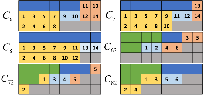
Figure 1. The tableaux of the chain decomposition of $L(3,8)$ under $\varphi$.

By investigating these chain tableaux of $L(3,n)$ for small $n$, we find the pattern as follows.

Theorem 11.

The bijection $\varphi$ in Theorem 3 produces a chain decomposition of $L(3,n)$. The corresponding chain tableaux are divided into two types: i) $C_{\mu}$ with $\mu=(4k,2k,0)$ for $k=0,1,\dots,\lfloor n/4\rfloor$, as in Figure 2; ii) $C_{\mu}$ with $\mu=(4k+\ell,2k,0)$ where $\ell\geq 2$ and $k=0,1,\dots,\lfloor(n-\ell)/4\rfloor$, as in Figure 3.

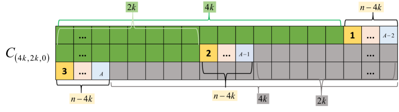
Figure 2. Chain tableaux of Type i) starting at $\mu=(4k,2k,0)$, where $A=3n-12k$.

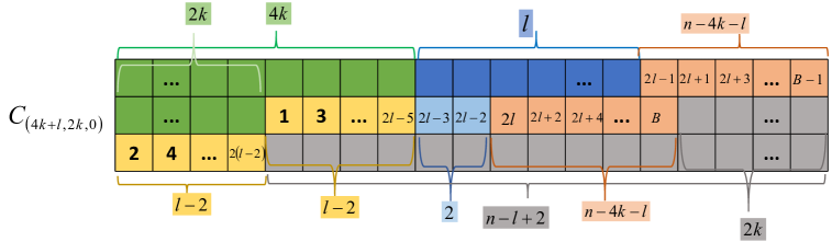
Figure 3. Chain tableaux of Type ii) starting at $\mu=(4k,2k,\ell)$ where $\ell\geq 2$ and $B=2n+4\ell-8k-2$.

We give two proofs of the theorem. The second proof will be given in the next section. The first proof need the following Lemma.

Lemma 12.

We have the following facts:

1. If $\lambda=(4k+c,2k+c,c),k\geqslant 0,c\geqslant 0$, then $\lambda\in E_{3,\lambda_{1}}$.

2. If $\lambda=(4k+c+1,2k+c,c),k\geqslant 1,c\geqslant 0$, then $\lambda\notin E_{3,\lambda_{1}}$,$\lambda_{2}+\lambda_{3}\equiv 0\pmod{2}$ and $(\lambda_{1}-1,\lambda_{2}+1,\lambda_{3})\notin E_{3,\lambda_{1}-1}$.

3. If $\lambda=(4k+c+1,2k+c+1,c),k\geqslant 1,c\geqslant 0$, then $\lambda\notin E_{3,\lambda_{1}}$, $\lambda_{2}+\lambda_{3}\not\equiv 0\pmod{2}$ and $(\lambda_{1}-1,\lambda_{2},\lambda_{3}+1)\notin E_{3,\lambda_{1}-1}$.

4. If $\lambda=(4k+\ell,2k+c,c),k\geqslant 0,1\leqslant c\leqslant\ell-2,\ell\geqslant 2$, then $\lambda\notin E_{3,\lambda_{1}}$,$\lambda_{2}+\lambda_{3}\equiv 0\pmod{2}$ and $(\lambda_{1}-1,\lambda_{2}+1,\lambda_{3})\notin E_{3,\lambda_{1}-1}$.

5. If $\lambda=(4k+\ell,2k+c+1,c),k\geqslant 0,1\leqslant c\leqslant\ell-3,\ell\geqslant 2$, then $\lambda\notin E_{3,\lambda_{1}}$, $\lambda_{2}+\lambda_{3}\not\equiv 0\pmod{2}$ and $(\lambda_{1}-1,\lambda_{2},\lambda_{3}+1)\notin E_{3,\lambda_{1}-1}$.

6. If $\lambda=(4k+\ell+c,2k+\ell+c,\ell-2),c\geqslant 0,k\geqslant 0,\ell\geqslant 2$, then $\lambda\in E_{3,\lambda_{1}}$.

7. If $\lambda=(4k+\ell+c+1,2k+\ell+c,\ell-2),k\geqslant 0,c\geqslant 0,\ell\geqslant 2$, then $\lambda\notin E_{3,\lambda_{1}}$ and $\lambda$ satisfy one of the following two conditions:
   (1) $\lambda_{2}+\lambda_{3}\equiv 0\pmod{2}$ and $(\lambda_{1}-1,\lambda_{2}+1,\lambda_{3})\notin E_{3,\lambda_{1}-1}$;
   (2) $\lambda_{2}+\lambda_{3}\not\equiv 0\pmod{2}$ and $(\lambda_{1}-1,\lambda_{2},\lambda_{3}+1)\in E_{3,\lambda_{1}-1}$.

Proof.

1. Direct calculation gives $\lambda_{1}-\lambda_{2}=2k$ and $2\lambda_{2}-\lambda_{1}-\lambda_{3}=0\in\mathbb{N}\setminus\{1\}$.

2. By direct calculation, $\lambda_{1}-\lambda_{2}=2k+1$ is odd, which implies $\lambda\notin E_{3,\lambda_{1}}$; $\lambda_{2}+\lambda_{3}=2k+2c$ is even; Let $\rho=(\lambda_{1}-1,\lambda_{2}+1,\lambda_{3})$. Then $\rho_{1}-\rho_{2}=2k-1$ is odd, which implies that $\rho\notin E_{3,\lambda_{1}-1}$.

3. By direct calculation, $2\lambda_{2}-\lambda_{1}-\lambda_{3}=1\notin\mathbb{N}\setminus\{1\}$, which implies $\lambda\notin E_{3,\lambda_{1}}$; $\lambda_{2}+\lambda_{3}=2k+2c+1$ is odd; Let $\rho=(\lambda_{1}-1,\lambda_{2},\lambda_{3}+1)$. Then $\rho_{1}-\rho_{2}=2k-1$ implies $\rho\notin E_{3,\lambda_{1}-1}$.

4. By $2\lambda_{2}-\lambda_{1}-\lambda_{3}=-(\ell-c)(\leq-2)\notin\mathbb{N}\setminus\{1\}$ we have $\lambda\notin E_{3,\lambda_{1}}$; $\lambda_{2}+\lambda_{3}=2k+2c$ is even; Let $\rho=(\lambda_{1}-1,\lambda_{2}+1,\lambda_{3})$. Then $2\rho_{2}-\rho_{1}-\rho_{3}=-(\ell-c)\leq-2$ and is hence not in $\mathbb{N}\setminus\{1\}$, so that $\rho\notin E_{3,\lambda_{1}-1}$.

5. By $2\lambda_{2}-\lambda_{1}-\lambda_{3}=-(\ell-c)+2(\leq-1)\notin\mathbb{N}\setminus\{1\}$ we have $\lambda\notin E_{3,\lambda_{1}}$; $\lambda_{2}+\lambda_{3}=2k+2c+1$ is odd; Let $\rho=(\lambda_{1}-1,\lambda_{2},\lambda_{3}+1)$. Then $2\rho_{2}-\rho_{1}-\rho_{3}=-(\ell-c)+1(\leq-2)\notin\mathbb{N}\setminus\{1\}$, so that $\rho\notin E_{3,\lambda_{1}-1}$.

6. Since $\lambda_{1}-\lambda_{2}=2k$ is even and $2\lambda_{2}-\lambda_{1}-\lambda_{3}=2c+2\in\mathbb{N}\setminus\{1\}$, we have $\lambda\in E_{3,\lambda_{1}}$.

7. By $\lambda_{1}-\lambda_{2}=2k+1$ we have $\lambda\notin E_{3,\lambda_{1}}$.

   (1) If $\lambda_{2}+\lambda_{3}=2k+2\ell+c-2$ is even. Let $\rho=(\lambda_{1}-1,\lambda_{2}+1,\lambda_{3})=(4k+\ell+c,2k+\ell+c+1,\ell-2)$. Then $\rho_{1}-\rho_{2}=2k-1$ is odd, so that $\rho\notin E_{3,\lambda_{1}-1}$.

   (2) If $\lambda_{2}+\lambda_{3}=2k+2\ell+c-2$ is odd. Let $\rho=(\lambda_{1}-1,\lambda_{2},\lambda_{3}+1)=(4k+\ell+c,2k+\ell+c,\ell-1)$. Then $\rho_{1}-\rho_{2}=0$ is even. Since $\lambda_{2}+\lambda_{3}=2k+2\ell+c-2$ is odd, we have $c\neq 0$ and therefore $2\rho_{2}-\rho_{1}-\rho_{3}=c+1\in\mathbb{N}\setminus\{1\}$.

 

First proof of Theorem 11.

We prove by applying Lemma 12 and the definition of $\varphi$. There are two cases as follows.

1. See Figure 2. For each $k,c\in\mathbb{N}$, let $\mu_{c}=(\mu_{1},\mu_{2},\mu_{3})=(4k+c,2k+c,c)$. By Lemma 12 part $(A_{1})$, $(A_{2})$ and $(A_{3})$, we get $\varphi(\mu_{c})=(\mu_{1}+1,\mu_{2},\mu_{3})=(4k+c+1,2k+c,c)$, $\varphi^{2}(\mu_{c})=(\mu_{1}+1,\mu_{2}+1,\mu_{3})=(4k+c+1,2k+c+1,c)$ and $\varphi^{3}(\mu_{c})=(\mu_{1}+1,\mu_{2}+1,\mu_{3}+1)=(4k+c+1,2k+c+1,c+1)$ respectively.

2. See Figure 3. First consider labels up to $2\ell-5$. For each $k\in\mathbb{N}$ and $\ell\geqslant 2$ satisfying $1\leqslant c\leqslant\ell-3$, let $\nu_{\ell,c}=(4k+\ell,2k+c,c)$. By part $(B_{2})$ and $(B_{3})$, we have

   $$\nu_{\ell,c}\mathop{\longrightarrow}\limits^{\varphi}(4k+\ell,2k+c+1,c)\mathop{\longrightarrow}\limits^{\varphi}(4k+\ell,2k+c+1,c+1)=\nu_{\ell,c+1}.$$

   This process end at $\omega=\nu_{\ell,\ell-2}=(4k+\ell,2k+\ell-2,\ell-2)$ with label $2\ell-4$.

   Next consider $\omega$ with label $2\ell-4$ and $\rho=(4k+\ell,2k+\ell-1,\ell-2)$ with label $2\ell-3$. By part $(B_{2})$, we get $\varphi(\omega)=\rho$, as desired. We need to show that $\rho\in F_{2}^{o}$ so that $\varphi(\rho)=(4k+\ell,2k+\ell,\ell-2)$ DO corresponds to label $2\ell-2$. Firstly $\rho_{2}+\rho_{3}=2k+2\ell-3$ is odd; Secondly let $\tau=(\rho_{1}-1,\rho_{2},\rho_{3}+1)$. Then $\tau_{1}-\tau_{2}=2k$ is even and $2\tau_{2}-\tau_{1}-\tau_{3}=0\in\mathbb{N}\setminus\{1\}$, so that $\tau\in E_{3,\rho_{1}-1}$; Finally $\rho_{1}-\rho_{2}=2k+1$ is odd, which implies that $\rho\notin E_{3,\rho_{1}}$.

   For labels begin at $2\ell-2$, let $\mu_{\ell,c}=(4k+\ell+c,2k+\ell+c,\ell-2)$, where $k\in\mathbb{N}$ and $\ell\geqslant 2$ satisfy $0\leqslant c\leqslant n-4k-\ell-1$. By part $(C_{1})$ and $(C_{2})$, we have

   $$\qquad\mu_{\ell,c}\mathop{\longrightarrow}\limits^{\varphi}(4k+\ell+c+1,2k+\ell+c,\ell-2)\\ \mathop{\longrightarrow}\limits^{\varphi}(4k+\ell+c+1,2k+\ell+c+1,\ell-2)=\mu_{\ell,c+1}.\qquad$$

   This process ends at $\mu_{\ell,n-4k-\ell}=(n,n-2k,\ell-2)$.

 

From the proof, we see that $\varphi$ induces two type of chains: i) Chains from $(4k,2k,0)$ to $(n,n-2k,n-4k)=(4k,2k,0)^{*}$; ii) For $\ell\geq 2$, we have chains from $(4k+\ell,2k,0)$ to $(n,n-2k,\ell-2)=(n-\ell+2,2k,0)^{*}$. This give rise an involution $\psi$ on $S_{3,n}$ defined by $\psi((4k,2k,0))=(4k,2k,0)$ and $\psi((4k+\ell,2k,0))=(n-\ell+2,2k,0)$ for $\ell\geq 2$. The fixed points of $\psi$ are $\{(4k,2k,0):4k\leq n\}\cup\{(4k+\ell,2k,0):\ell\geq 2,n=4k+2\ell-2\}$.

3.1. Comparison with other chain decompositions

In Figure 4 we draw the tableaux of the symmetric chain decompositions of $L(3,6)$ from a result of Bernt Lindstr$\ddot{o}$m [1]. Compare it with our chain decompositions in Figure 5. We also draw the tableaux of the symmetric chain decompositions of $L(4,4)$ from a result of Douglas B. West [8] in Figure 6. Compare it with our chain decompositions in Figure 7. In both examples, the pattern of our chain decompositions seems easier to find.

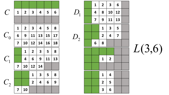
Figure 4. The tableaux for Lindstr$\ddot{o}$m’s chain decompositions of $L(3,6)$.

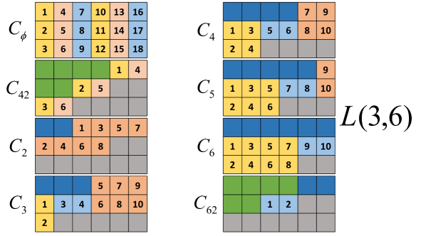
Figure 5. The tableaux for our chain decompositions of $L(3,6)$.

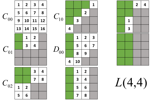
Figure 6. The tableaux for West’s chain decompositions of $L(4,4)$.

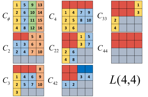
Figure 7. The tableaux for our chain decompositions of $L(4,4)$.

4. Sperner chain decompositions of $L(3,n)$ and $L(4,n)$

A chain decomposition $C_{1},C_{2},\dots,C_{N}$ of $L(m,n)$ is called Sperner if it satisfies the following two conditions: i) $L(m,n)$ is the disjoint union of the $C_{j}$’s; ii) each $C_{j}$ is of the form $x_{j,1}<x_{j,2}<x_{j,3}<\cdots<x_{j,e_{j}}$ with $\operatorname{rank}(x_{j,1})\leq mn/2$ and $\operatorname{rank}(x_{j,e_{j}})\geq mn/2$, where $x_{j,1}$ are called the starting partitions and $x_{j,e_{j}}$ are called the end partitions. Obviously each $C_{j}$ intersects $L_{\lfloor mn/2\rfloor}(m,n)$, which implies the Sperner property. Symmetric chain decompositions are Sperner chain decompositions satisfying the extra rank symmetric condition $\operatorname{rank}(x_{j,1})+\operatorname{rank}(x_{j,e_{j}})=mn$.

Theorem 11 indeed give a Sperner chain decomposition of $L(3,n)$. Its first proof relies on the order matching $\varphi$. We give a self-contained proof and extend the result for $L(4,n)$.

4.1. A direct proof for the chain decomposition of $L(3,n)$

We need the following classification of $L(3,n)$ in 7 types.

Lemma 13.

Any element $\lambda=(\lambda_{1},\lambda_{2},\lambda_{3})$ in $L(3,n)$ can be uniquely expressed in one of the following forms:

1. $(4k+c,2k+c,c),\ k\geqslant 0,\ c\geqslant 0$.

2. $(4k+c+1,2k+c,c),\ k\geqslant 0,\ c\geqslant 0$.

3. $(4k+c+1,2k+c+1,c),\ k\geqslant 0,\ c\geqslant 0$.

4. $(4k+\ell,2k+c,c),\ k\geqslant 0,\ \ell\geqslant 2,\ \ell-2\geqslant c\geqslant 0$.

5. $(4k+\ell,2k+c+1,c),\ k\geqslant 0,\ \ell\geqslant 2,\ \ell-2\geqslant c\geqslant 0$.

6. $(4k+\ell+c,2k+\ell+c,\ell-2),\ k\geqslant 0,\ \ell\geqslant 2,\ c\geqslant 0$.

7. $(4k+\ell+c+1,2k+\ell+c,\ell-2),\ k\geqslant 0,\ \ell\geqslant 2,\ c\geqslant 0$.

Proof.

We first prove the uniqueness. Since the elements in each type are clearly different from each other, it suffices to prove that there are no identical elements between different types. This is achieved by computing the values $\alpha=\lambda_{1}-\lambda_{2}$, $\beta=\lambda_{2}-\lambda_{3}$, and $\alpha-\beta$ for each $\lambda$, as given in the following table.

$$\begin{array}[]{|l|l|l|l|l|}\hline\cr&(\lambda_{1},\lambda_{2},\lambda_{3})&\alpha-\beta&\alpha=\lambda_{1}-\lambda_{2}&\beta=\lambda_{2}-\lambda_{3}\\ \hline\cr A_{1})&(4k+c,2k+c,c)&0&even&even\\ \hline\cr A_{2})&(4k+c+1,2k+c,c)&1&odd&even\\ \hline\cr A_{3})&(4k+c+1,2k+c+1,c)&-1&even&odd\\ \hline\cr B_{2})&(4k+\ell,2k+c,c)&\ell-c\geq 2&&even\\ \hline\cr B_{3})&(4k+\ell,2k+c+1,c)&\ell-c-2\geq 0&&odd\\ \hline\cr C_{1})&(4k+\ell+c,2k+\ell+c,\ell-2)&-2-c\leq-2&even&\\ \hline\cr C_{2})&(4k+\ell+c+1,2k+\ell+c,\ell-2)&-1-c\leq-1&odd&\\ \hline\cr\end{array}$$

For instance, type $A_{1}$ and $B_{3}$ partitions can only overlap at $\lambda$ with $\alpha-\beta=0$, but their $\beta$ values have different parity. The other cases can be done similarly.

Next we prove that any element in $L(3,n)$ belongs to one of the seven types. Let $\alpha$ and $\beta$ be defined as above for a given $\lambda=(\lambda_{1},\lambda_{2},\lambda_{3})$. The following table determines the type of $\lambda$ and their corresponding representations.

$$\begin{array}[]{|l|l|l|l|l|l|l|}\hline\cr\alpha-\beta&\alpha&\beta&k&c&\ell&\text{type of }\lambda\\ \hline\cr 0&even&even&\frac{\alpha}{2}&\lambda_{3}&\times&A_{1})\\ \hline\cr 1&odd&even&\frac{\beta}{2}&\lambda_{3}&\times&A_{2})\\ \hline\cr-1&even&odd&\frac{\alpha}{2}&\lambda_{3}&\times&A_{3})\\ \hline\cr\geq 2&&even&\frac{\beta}{2}&\lambda_{3}&(\alpha-\beta)+\lambda_{3}&B_{2})\\ \hline\cr\geq 0&&odd&\frac{\beta-1}{2}&\lambda_{3}&(\alpha-\beta)+\lambda_{3}+2&B_{3})\\ \hline\cr\leq-2&even&&\frac{\alpha}{2}&-(\alpha-\beta)-2&\lambda_{3}+2&C_{1})\\ \hline\cr\leq-1&odd&&\frac{\alpha-1}{2}&-(\alpha-\beta)-1&\lambda_{3}+2&C_{2})\\ \hline\cr\end{array}.$$

This completes the proof.  

Second proof of Theorem 11.

The theorem clearly follows by the following Claims 1 and 2.

Claim 1: For each $k$, $C_{\mu}$ with $\mu=(4k,2k,0)$ contains elements of type $A$ for all $c$.

Starting at the $A_{1}$ element $(4k,2k,0)$ with $c=0$, we successively add $1$ to the first row, the second row and the third row to get $A_{2}$, $A_{3}$, and $A_{1}$ elements respectively. Now we are at the $A_{1}$ element $(4k+1,2k+1,1)$ with $c=1$. Continuing this way, we see that Claim 1 holds true.

Claim 2: For each $k$ and $\ell\geq 2$, $C_{\mu}$ with $\mu=(4k+\ell,2k,0)$ contains all elements of type $B$ and $C$ for all $c$.

Starting at $B_{2}$ element $(4k+\ell,2k,0)$ with $c=0$, we successively add $1$ to the second row, and the third row to get $B_{3}$ and $B_{2}$ elements respectively. Now we are at the $B_{2}$ element $(4k+\ell,2k+1,1)$ with $c=1$. Continuing this way until we reach the $B_{2}$ element $(4k+\ell,2k+\ell-2,\ell-2)$ with $c=\ell-2$. By adding $1$ to the second row, we get the $B_{3}$ element $(4k+\ell,2k+\ell-1,\ell-2)$ with $c=\ell-2$. This covers all type $B$ elements.

Next we add $1$ to the second row to get the $C_{1}$ element $(4k+\ell,2k+\ell,\ell-2)$ with $c=0$. After that, we successively add $1$ to the first row, and the second row to get $C_{2}$ and $C_{1}$ elements respectively. Now we are at the $C_{1}$ element $(4k+\ell+1,2k+\ell+1,\ell-2)$ with $c=1$. Continuing this way, we see that Claim 2 holds true.  

4.2. Sperner chain decompositions of $L(4,n)$

Our chain decompositions for $L(4,n)$ are also from the greedy algorithm. Let us see Figure 8 for the Chain tableaux of $L(4,8)$ for the pattern.

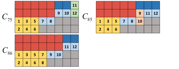
Figure 8. The tableaux of all $L(4,8)$ chains.

For general $n$, the result is summarized as follows.

Theorem 14.

The Young’s lattice $L(4,n)$ is a disjoint union of chains, where the corresponding chain tableaux are divided into four types:

A) $C_{\mu}$ with $\mu=(6k,4k,2k,0)$ for $k=0,1,\dots,\lfloor n/6\rfloor$, as in Figure 9. Partitions in these chains will be called of type $A_{1},A_{2},A_{3},A_{4}$;

B) $C_{\mu}$ with $\mu=(6k+\ell,4k+\ell,2k,0)$, where $\ell\geq 2$ and $k=0,1,\dots,\lfloor(n-\ell)/6\rfloor$, as in Figure 10. Partitions in these chains will be called of type $B_{1},B_{3},B_{2},B_{4}$;

C) $C_{\mu}$ with $\mu=(6k+r,4k,2k,0)$, where $r\geq 2$ and $k=0,1,\dots,\lfloor(n-r)/6\rfloor$, as in Figure 11. Partitions in these chains will be called of type $C_{a2},C_{a3},C_{a4},C_{b2},C_{b_{3}},C_{b1}$;

D) $C_{\mu}$ with $\mu=(6k+r+\ell,4k+\ell,2k,0)$, where $\ell\geq 2$, $r\geq 2$ and $k=0,1,\dots,\lfloor(n-r-\ell)/6\rfloor$, as in Figure 12. Partitions in these chains will be called of type
$D_{a3},D_{a4},D_{b2},D_{b3},D_{c1},D_{c2}$.

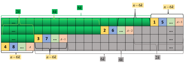
Figure 9. Chain tableaux of Type i) starting at $\mu=(6k,4k,2k,0)$, $k\in\mathbb{N}$, where $A=4n-24k$.

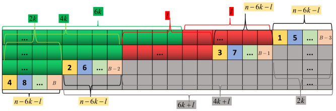
Figure 10. Chain tableaux of Type ii) starting at $\mu=(6k+\ell,4k+\ell,2k,0)$, $k\in\mathbb{N}$,$\ell\geq 2$, where $B=4n-24k-4\ell$.

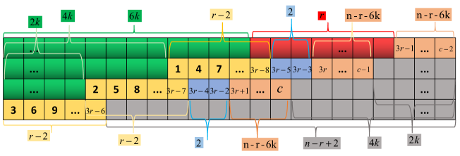
Figure 11. Chain tableaux of Type iii) starting at $\mu=(6k+r,4k,2k,0)$, $k\in\mathbb{N}$,$r\geq 2$, where $C=3n-18k-2$.

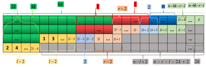
Figure 12. Chain tableaux of Type iv) starting at $\mu=(6k+r+\ell,4k+\ell,2k,0)$, $k\in\mathbb{N}$,$r\geq 2$,$\ell\geq 2$, where $D=2\ell+2r-7$ and $E=2n-12k-5$.

The proof of Theorem 14 is similar to that of Theorem 11. We only sketch the idea.

We divide partitions in $L(4,n)$ as in the following lemma.

Lemma 15.

Any element $\lambda=(\lambda_{1},\lambda_{2},\lambda_{3},\lambda_{4})$ in $L(4,n)$ can be expressed in one of the following forms:

1. $(6k+c,4k+c,2k+c,c),k\geqslant 0,n-6k\geqslant c\geqslant 0$.

2. $(6k+c+1,4k+c,2k+c,c),k\geqslant 0,n-6k-1\geqslant c\geqslant 0$.

3. $(6k+c+1,4k+c+1,2k+c,c),k\geqslant 0,n-6k-1\geqslant c\geqslant 0$.

4. $(6k+c+1,4k+c+1,2k+c+1,c),k\geqslant 0,n-6k-1\geqslant c\geqslant 0$.

5. $(6k+\ell+c,4k+\ell+c,2k+c,c),k\geqslant 0,\ell\geqslant 2,n-6k-\ell\geqslant c\geqslant 0$.

6. $(6k+\ell+c+1,4k+\ell+c,2k+c,c),k\geqslant 0,\ell\geqslant 2,n-6k-\ell-1\geqslant c\geqslant 0$.

7. $(6k+\ell+c+1,4k+\ell+c,2k+c+1,c),k\geqslant 0,\ell\geqslant 2,n-6k-\ell-1\geqslant c\geqslant 0$.

8. $(6k+\ell+c+1,4k+\ell+c+1,2k+c+1,c),k\geqslant 0,\ell\geqslant 2,n-6k-\ell-1\geqslant c\geqslant 0$.

9. $(6k+r,4k+c,2k+c,c),k\geqslant 0,r\geqslant 2,r-2\geqslant c\geqslant 0$.

10. $(6k+r,4k+c+1,2k+c,c),k\geqslant 0,r\geqslant 2,r-2\geqslant c\geqslant 0$.

11. $(6k+r,4k+c+1,2k+c+1,c),k\geqslant 0,r\geqslant 2,r-3\geqslant c\geqslant 0$.

12. $(6k+r+c,4k+r-1+c,2k+r-1+c,r-2),k\geqslant 0,r\geqslant 2,n-r-6k\geqslant c\geqslant 0$.

13. $(6k+r+c,4k+r+c,2k+r-1+c,r-2),k\geqslant 0,r\geqslant 2,n-r-6k\geqslant c\geqslant 0$.

14. $(6k+r+c,4k+r+c,2k+r+c,r-2),k\geqslant 0,r\geqslant 2,n-r-6k\geqslant c\geqslant 0$.

15. $(6k+\ell+r,4k+\ell,2k+c,c),k\geqslant 0,\ell\geqslant 2,r\geqslant 2,\ell-2\geqslant c\geqslant 0$.

16. $(6k+\ell+r,4k+\ell,2k+c+1,c),k\geqslant 0,\ell\geqslant 2,r\geqslant 2,\ell-2\geqslant c\geqslant 0$.

17. $(6k+\ell+r,4k+\ell+c,2k+\ell+c,\ell-2),k\geqslant 0,\ell\geqslant 2,r\geqslant 2,r-2\geqslant c\geqslant 0$.

18. $(6k+\ell+r,4k+\ell+c+1,2k+\ell+c,\ell-2),k\geqslant 0,\ell\geqslant 2,r\geqslant 2,r-2\geqslant c\geqslant 0$.

19. $(6k+\ell+r+c,4k+\ell+r+c,2k+\ell+r-2,\ell-2),k\geqslant 0,\ell\geqslant 2,r\geqslant 2,n-6k-r-\ell\geqslant c\geqslant 0$.

20. $(6k+\ell+r+c+1,4k+\ell+r+c,2k+\ell+r-2,\ell-2),k\geqslant 0,\ell\geqslant 2,r\geqslant 2,n-6k-r-\ell-1\geqslant c\geqslant 0$.

Proof.

Clearly partitions in each type are different from each other. To show that partitions from different types can not equal, we compute in the following table, where for $\lambda=(\lambda_{1},\lambda_{2},\lambda_{3},\lambda_{4})$, we define $\alpha=\lambda_{1}-\lambda_{2},\beta=\lambda_{2}-\lambda_{3},\gamma=\lambda_{3}-\lambda_{4}$. The proof is completed by data in Figures 13, 14, 15, and 16.

$$\begin{array}[]{|l|l|l|l|l|l|l|}\hline\cr\lambda&\alpha-\beta&\alpha-\gamma&\beta-\gamma&\alpha&\beta&\gamma\\ \hline\cr A_{1})&0&0&0&even&even&even\\ \hline\cr A_{2})&1&1&0&odd&even&even\\ \hline\cr A_{3})&-1&0&1&even&odd&even\\ \hline\cr A_{4})&0&-1&-1&even&even&odd\\ \hline\cr B_{1})&-\ell\leqslant-2&0&\ell\geqslant 2&even&&even\\ \hline\cr B_{3})&1-\ell\leqslant-1&1&\ell\geqslant 2&odd&&even\\ \hline\cr B_{2})&2-\ell\leqslant 0&0&\ell-2\geqslant 0&odd&&odd\\ \hline\cr B_{4})&-\ell\leqslant-2&-1&\ell-1\geqslant 1&even&&odd\\ \hline\cr C_{a2})&r-c\geqslant 2&r-c\geqslant 2&0&&even&even\\ \hline\cr C_{a3})&r-c-2\geqslant 0&r-c-1\geqslant 1&1&&odd&even\\ \hline\cr C_{a4})&r-c-1\geqslant 2&r-c-2\geqslant 1&-1&&even&odd\\ \hline\cr C_{b2})&1&-c\leqslant-1&-1-c\leqslant-1&odd&even&\\ \hline\cr C_{b3})&-1&-1-c\leqslant-1&-c\leqslant 0&even&odd&\\ \hline\cr C_{b1})&0&-2-c\leqslant-2&-2-c\leqslant-2&even&even&\\ \hline\cr D_{a3})&r-\ell+c&r\geqslant 2&\ell-c\geqslant 2&&&even\\ \hline\cr D_{a4})&r-\ell+c+1&r-1\geqslant 1&\ell-c-2\geqslant 0&&&odd\\ \hline\cr D_{b2})&r-c\geqslant 2&r-2c-2&-2-c\leqslant-2&&even&\\ \hline\cr D_{b3})&r-c-2\geqslant 0&r-2c-3&-1-c\leqslant-1&&odd&\\ \hline\cr D_{c1})&-2-c\leqslant-2&-r\leqslant-2&c+2-r&even&&\\ \hline\cr D_{c2})&-1-c\leqslant-1&1-r\leqslant-1&c+2-r&odd&&\\ \hline\cr\end{array}$$

Figure 13. The $\alpha,\beta,\gamma$ values for different types.

Figure 14. Proof of the distinction of partitions from different types.

$$\begin{array}[]{|l|l|l|l|l|l|l|}\hline\cr\alpha-\beta&\alpha-\gamma&\beta-\gamma&\alpha&\beta&\gamma&\lambda\\ \hline\cr 0&0&0&even&even&even&A_{1}\\ \hline\cr 1&1&0&odd&even&even&A_{2}\\ \hline\cr-1&0&1&even&odd&even&A_{3}\\ \hline\cr 0&-1&-1&even&even&odd&A_{4}\\ \hline\cr\leqslant-2&0&\geqslant 2&even&&even&B_{1}\\ \hline\cr\leqslant-1&1&\geqslant 2&odd&&even&B_{3}\\ \hline\cr\leqslant 0&0&\geqslant 0&odd&&odd&B_{2}\\ \hline\cr\leqslant-2&-1&\geqslant 1&even&&odd&B_{4}\\ \hline\cr\geqslant 2&\geqslant 2&0&&even&even&C_{a2}\\ \hline\cr\geqslant 0&\geqslant 1&1&&odd&even&C_{a3}\\ \hline\cr\geqslant 2&\geqslant 1&-1&&even&odd&C_{a4}\\ \hline\cr 1&\leqslant 0&\leqslant-1&odd&even&&C_{b2}\\ \hline\cr-1&\leqslant-1&\leqslant 0&even&odd&&C_{b3}\\ \hline\cr 0&\leqslant-2&\leqslant-2&even&even&&C_{b1}\\ \hline\cr&\geqslant 2&\geqslant 2&&&even&D_{a3}\\ \hline\cr&\geqslant 1&\geqslant 0&&&odd&D_{a4}\\ \hline\cr\geqslant 2&&\leqslant-2&&even&&D_{b2}\\ \hline\cr\geqslant 0&&\leqslant-1&&odd&&D_{b3}\\ \hline\cr\leqslant-2&\leqslant-2&&even&&&D_{c1}\\ \hline\cr\leqslant-1&\leqslant-1&&odd&&&D_{c2}\\ \hline\cr\end{array}$$

Figure 15. Determine the types from the $\alpha,\beta,\gamma$ values.

$$\begin{array}[]{|l|l|l|l|l|}\hline\cr\lambda&k&\ell&r&c\\ \hline\cr A_{1}&\frac{\alpha}{2}&\times&\times&\lambda_{4}\\ \hline\cr A_{2}&\frac{\beta}{2}&\times&\times&\lambda_{4}\\ \hline\cr A_{3}&\frac{\alpha}{2}&\times&\times&\lambda_{4}\\ \hline\cr A_{4}&\frac{\alpha}{2}&\times&\times&\lambda_{4}\\ \hline\cr B_{1}&\frac{\alpha}{2}&-(\alpha-\beta)&\times&\lambda_{4}\\ \hline\cr B_{3}&\frac{\alpha-1}{2}&-(\alpha-\beta)+1&\times&\lambda_{4}\\ \hline\cr B_{2}&\frac{\alpha-1}{2}&-(\alpha-\beta)+2&\times&\lambda_{4}\\ \hline\cr B_{4}&\frac{\alpha}{2}&-(\alpha-\beta)&\times&\lambda_{4}\\ \hline\cr C_{a2}&\frac{\beta}{2}&\times&(\alpha-\beta)+\lambda_{4}&\lambda_{4}\\ \hline\cr C_{a3}&\frac{\beta-1}{2}&\times&(\alpha-\beta)+\lambda_{4}+2&\lambda_{4}\\ \hline\cr C_{a4}&\frac{\beta}{2}&\times&\lambda_{4}+2&\lambda_{4}\\ \hline\cr C_{b2}&\frac{\beta}{2}&\times&\lambda_{4}+2&-(\beta-\gamma)-1\\ \hline\cr C_{b3}&\frac{\alpha}{2}&\times&\lambda_{4}+2&-(\alpha-\gamma)-1\\ \hline\cr C_{b1}&\frac{\alpha}{2}&\times&\lambda_{4}+2&-(\alpha-\gamma)-2\\ \hline\cr D_{a3}&\frac{\gamma}{2}&(\beta-\gamma)+\lambda_{4}&(\alpha-\gamma)&\lambda_{4}\\ \hline\cr D_{a4}&\frac{\gamma-1}{2}&(\beta-\gamma)+\lambda_{4}+2&(\alpha-\gamma)+1&\lambda_{4}\\ \hline\cr D_{b2}&\frac{\beta}{2}&\lambda_{4}+2&(\alpha-\beta)-(\beta-\gamma)-2&-(\beta-\gamma)-2\\ \hline\cr D_{b3}&\frac{\beta-1}{2}&\lambda_{4}+2&(\alpha-\beta)-(\beta-\gamma)+1&-(\beta-\gamma)-1\\ \hline\cr D_{c1}&\frac{\alpha}{2}&\lambda_{4}+2&(\alpha-\gamma)&-(\alpha-\beta)-2\\ \hline\cr D_{c2}&\frac{\alpha-1}{2}&\lambda_{4}+2&(\alpha-\gamma)+1&-(\alpha-\beta)-1\\ \hline\cr\end{array}$$

Figure 16. From the types and $\alpha,\beta,\gamma$ values to the partitions.

 

5. Recursive Sperner chain decompositions of $L(m,n)$

A basic idea is that by using the dual operation, we only need the upper half part of $L(m,n)$ to construct the a Sperner chain decomposition.

Definition 16.

$L^{U}(m,n)=:\{\lambda\mid\lambda\in L(m,n),\left|\lambda\right|\leq d_{m,n},\ d_{m,n}=\left\lfloor\frac{mn+1}{2}\right\rfloor\}$.

Definition 17.

A U-decomposition of $L^{U}(m,n)$ is a chain decomposition $C_{1},C_{2},\cdots,C_{k}$, where $C_{i}=\lambda_{i,1}\leq\lambda_{i,2}\leq\cdots\leq\lambda_{i,t_{i}},\ i=1,2,\cdots,k$ satisfy the following conditions:

(1) $L^{U}(m,n)=C_{1}\cup C_{2}\cup\cdots\cup C_{k}$;

(2) $C_{1},C_{2},\cdots,C_{k}$ are disjoint;

(3) $\operatorname{rank}(\lambda_{i,t_{i}})=d_{m,n}$.

Example 18.

The U decompositions of $L^{U}(2,5)$ and $L^{U}(2,8)$ are given in Figure 17.

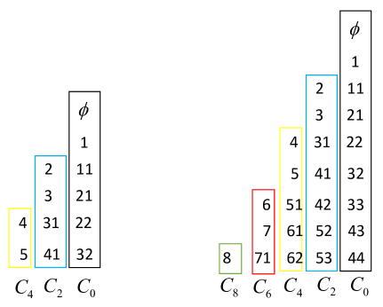
Figure 17. The U decomposition of $L^{U}(2,5)$ and $L^{U}(2,8)$.

Clearly, the dual of a U-decomposition of $L^{U}(m,n)$ is also a chain decomposition, but of the lower half of $L(m,n)$. We can knead them together to obtain a Sperner chain decomposition of $L(m,n)$.

Lemma 19.

If $L^{U}(m,n)$ has a U-decomposition $\{C_{1},C_{2},\cdots,C_{k}\}$, where $C_{i}$ is $\lambda_{i,1}\leq\lambda_{i,2}\leq\cdots\leq\lambda_{i,t_{i}}(i=1,2,\cdots,k)$, then $L(m,n)$ has a Sperner chain decomposition, and $\{\lambda_{i,1},i=1,2,\cdots,k\}$ is the starting set for the chain decomposition, $\{\lambda^{*}_{i,1},i=1,2,\cdots,k\}$ is the end point set of the chain decomposition.

Proof.

we discuss the parity of $mn$ as follows.

• When $mn$ is even, since the proposition $L(m,n)$ is rank-symmetric, we get $\{\lambda_{i,t_{i}},i=1,2,\cdots,k\}=\{\lambda^{*}_{i,t_{i}},i=1,2,\cdots,k\}$. So we knead the chain $C=\{C_{1},C_{2},\cdots,C_{k}\}$ and the chain $C^{\star}=\{C^{\star}_{1},C^{\star}_{2},\cdots,C^{\star}_{k}\}$ together to form a new chain denoted as $\tilde{C}=\{\tilde{C}_{1},\tilde{C}_{2},...,\tilde{C}_{k}\}$.

• When $mn$ is odd, since the proposition $L(m,n)$ is rank-symmetric, we get $\{\lambda_{i,t_{i}},i=1,2,\cdots,k\}=\{\lambda^{*}_{i,t_{i}-1},i=1,2,\cdots,k\}$. So we knead the chain $C=\{C_{1},C_{2},\cdots,C_{k}\}$ and the chain $C^{\star}=\{C^{\star}_{1},C^{\star}_{2},\cdots,C^{\star}_{k}\}$ together to form a new chain denoted as $\tilde{C}=\{\tilde{C}_{1},\tilde{C}_{2},\cdots,\tilde{C}_{k}\}$.

In a word, we get the Sperner chain decomposition $\tilde{C}=\{\tilde{C}_{1},\tilde{C}_{2},\cdots,\tilde{C}_{k}\}$ of $L(m,n)$.  

The above Lemma 19 is best explained by an example.

Example 20.

The U-decomposition of $L^{U}(3,3)$ is given by $C_{1},C_{2},C_{3}$. Then $C^{*}_{1},C^{*}_{2},C^{*}_{3}$ are constructed. We get the Sperner chain decomposition $\tilde{C}=\{\tilde{C}_{1},\tilde{C}_{3},\tilde{C}_{3}\}$ of $L(3,3)$. See Figure 18.

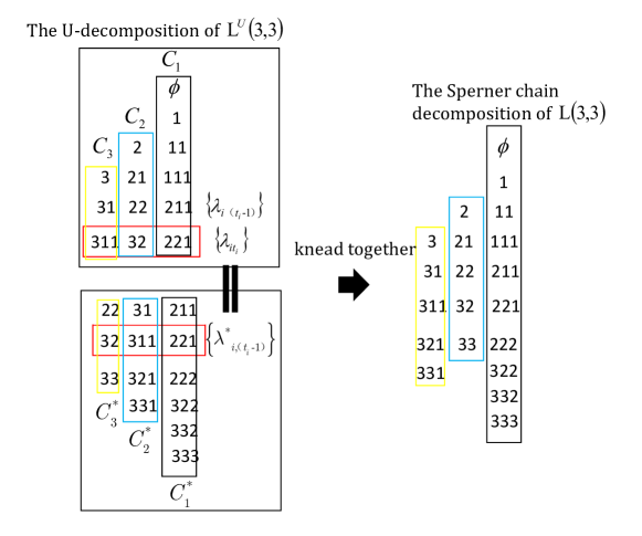
Figure 18. The knead process for $L(3,3)$.

5.1. The recursive construction

To decompose $L^{U}(m,n)$, we use the natural recursion $L(m,n)=L(m,n-1)\biguplus(n\oplus L(m-1,n))$, where $n\oplus(\lambda_{1},\dots,\lambda_{m-1})=(n,\lambda_{1},\dots,\lambda_{m-1})$ and $n\oplus L(m-1,n)=\{n\oplus\lambda:\lambda\in L(m-1,n)\}$.

Algorithm RecUD

Input: The U-decompositions of $L^{U}(m,n-1)$ and $L^{U}(m-1,n)$.
Output: The U-decomposition of $L^{U}(m,n)$ if possible.

1. Construct the Sperner Chain decomposition of $L(m,n-1)$ from the U-decomposition of $L^{U}(m,n-1)$. Chains end at a rank less than $d_{m,n}$ is called bad chains and need further operation. Other chains are cut at rank $d_{m,n}$ and kept as good chains. Let $E=\{\alpha^{1},\dots,\alpha^{e}\}$ be the set of end partitions of bad chains.

2. Map $\lambda$ to $n\bigoplus\lambda$ for all partitions in the U-decomposition of $L^{U}(m-1,n)$. Cut all chains at rank $d_{m,n}$. These are candidate chains for kneading with bad chains. Let $S=\{\beta^{1},\dots,\beta^{s}\}$ be the set of all starting partitions of these chains.

3. For each $\alpha^{i}$, add $1$ to the first entry and check if it equals $\beta^{j_{i}}$. If true for all $i$ then knead the bad chains with the corresponding candidate chains.

4. Good chains, kneaded candidate chains, and the remaining candidate chains form the U-decomposition of $L^{U}(m,n)$.

Example 21.

The U-decomposition of $L^{U}(3,5)$ is constructed in Figures 19,20,21,22.

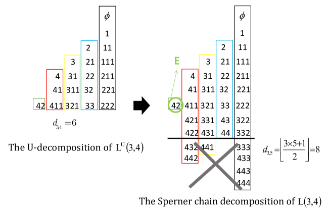
Figure 19. Step 1

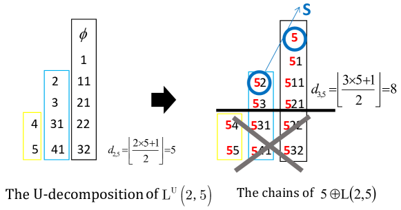
Figure 20. Step 2

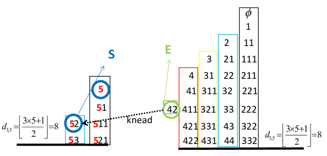
Figure 21. Step 3

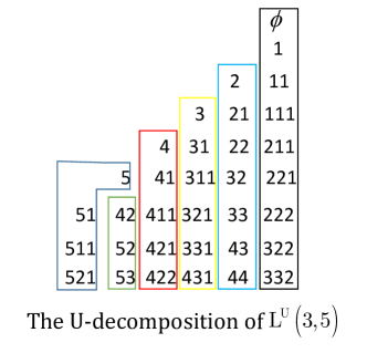
Figure 22. Step 4

From the algorithm, we see that the starting partitions play an important role. If we only want to show the existence of a Sperner chain decomposition, the algorithm maybe much simpler. Indeed, we can obtain the set $S_{m,n}$ of starting partitions .

Algorithm RecSmn

Input: The sets $S_{m,n-1}$ and $S_{m-1,n}$ of starting partitions for certain Sperner chain decompositions of $L(m,n-1)$ and $L(m-1,n)$, respectively.

Output: The set $S_{m,n}$ of starting partitions for a possible Sperner chain decomposition of $L(m,n)$.

1. Let $E_{m,n-1}=S_{m,n-1}^{*}$ be the set of end partitions of a Sperner chain decomposition of $L(m,n-1)$. Select all partitions of rank less than $d_{m,n}$ to form $E=\{\alpha^{1},\dots,\alpha^{e}\}$.

2. Let $S=n\bigoplus S_{m-1,n}=\{\beta_{1},\beta_{2},\dots\}$.

3. Add $1$ to the first entry for each $\alpha^{i}$ to obtain $E^{\prime}$. If $E^{\prime}\subseteq S$ then we can construct a Sperner chain decomposition of $L(m,n)$ with $S_{m,n}=S_{m,n-1}\bigcup S\setminus E^{\prime}$. Otherwise, the method failed.

The algorithm succeeds for $m\leq 4$.

Clearly, for $m=1$ $L(1,n)$ is a chain and we have $S_{1,n}=\{(0)\}$.

For $m=2$, we have

Proposition 22.

There is a Sperner chain decomposition for $L(2,n)$ with starting partitions $S_{2,n}=\{(2k,0):0\leq k\leq n/2\}$.

Proof.

The proposition clearly holds for $n=1$, in which case $L(2,1)$ itself is a chain.

Assume the proposition holds for $n$ and we want to show that it holds for $n+1$. We use Algorithm RecSmn and discuss by the parity of $n$: i) If $n$ is odd, then no elements in $E_{2,n}$ has rank less than $d_{2,n+1}$, so that $E=\emptyset$ and $S=(n+1)\oplus(0)$. It follows that $S_{2,n+1}=S_{2,n}\cup\{(n+1,0)\}$ as desired; ii) If $n$ is even, then only one element $(n,0)^{*}=(n,0)$ has rank less than $d_{2,n+1}=n+1$, so that $E=\{(n,0)\}$ and $S=(n+1)\oplus(0)$. Clearly we have the match $(n,0)\lessdot(n+1,0)$. It follows that $S_{2,n+1}=S_{2,n}$ as desired.  

For $m=3$, we have

Proposition 23.

There is a Sperner chain decomposition for $L(3,n)$ with starting partitions $S_{3,n}$ as in (2).

Proof.

To apply Algorithm RecSmn, it is better to have the following facts as guide for our proof.

1. $S_{3,4t}=S_{3,4t-1}\cup 4t\oplus\{(4t,0),(4t,2),(4t,4),\cdots,(4t,2t)\}$.

2. $S_{3,4t+1}=S_{3,4t}\cup(4t+1)\oplus\{(4t+1,0),(4t+1,2),(4t+1,4),\cdots,(4t+1,2t-2)\}$.

3. $S_{3,4t+2}=S_{3,4t+1}\cup(4t+2)\oplus\{(4t+2,0),(4t+2,2),(4t+2,4),\cdots,(4t+2,2t)\}$.

4. $S_{3,4t+3}=S_{3,4t+2}\cup(4t+3)\oplus\{(4t+3,0),(4t+3,2),(4t+3,4),\cdots,(4t+3,2t)\}$.

Case 1, for $(m,n)=(3,4t)$. We only need to consider starting partitions whose ranks $r$ satisfy $3\cdot(4t-1)-r<d_{3,4t}=6t$, which is equivalent to $r>6t-3$. By definition, we need all $(4k+\ell,2k,0)$ with $\ell\neq 1$ satisfying $6k+\ell>6t-3$ and $4k+\ell\leq 4t-1$, which simplifies to $t-\frac{\ell+3}{6}<k\leq t-\frac{\ell+1}{4}$. Since no such integer $k$ exists, $E$ is empty, and we have $S_{3,4t}=S_{3,4t-1}\cup((4t+1)\oplus S_{2,4t})$ as desired.

Case 2, for $(m,n)=(3,4t+1)$. We only need to consider starting partitions whose ranks $r$ satisfy $3\cdot 4t-r<d_{3,4t+1}=6t+2$, which is equivalent to $r>6t-2$. By definition, we need all $(4k+\ell,2k,0)$ with $\ell\neq 1$ satisfying $6k+\ell>6t-2$ and $4k+\ell\leq 4t$, which simplifies to $t-\frac{\ell+2}{6}<k\leq t-\frac{\ell}{4}$. This can happen only when $k=t$ and $\ell=0$. So $E=\{(4t,2t,0)^{*}\}=\{(4t,2t,0)\}$. Then $E^{\prime}=\{(4t+1,2t,0)\}\subseteq(4t+1)\oplus S_{2,4t+1}$. Hence we have $S_{3,4t+1}=S_{3,4t}\cup((4t+1)\oplus S_{2,4t+1})\setminus\{(4t+1,2t,0)\}$ as desired.

The other cases are similar.  

Theorem 24.

If we use the Sperner chain decomposition in Theorem 3, then Algorithm RecUD gives rise a Sperner chain decomposition of $L(4,n)$ with starting partitions

$$S_{4,n}=\{(6k+s+\ell,4k+\ell,2k,0):s,\ell,k\geq 0,\ s\neq 1,\ \ell\neq 1,\text{ and }6k+s+\ell\leq n\}.$$

Proof.

Case 1. We explain how to obtain $S_{4,6t+1}$ from $S_{4,6t}$.

We first need to find all starting partitions in $S_{4,6t}$ whose rank $r$ satisfy $4\cdot 6t-r<d_{4,6t+1}=12t+2$, which is $r>12t-2$. Let $(6k+s+\ell,4k+\ell,2k,0)$ be a such partition. Then we need the conditions: $12k+s+2\ell>12t-2$, $6k+s+\ell\leq 6t$, $s\neq 1$, $\ell\neq 1$. The first two inequalities are equivalent to $t-\frac{1+s+2\ell}{12}\leq k\leq t-\frac{s+\ell}{6}$, which implies $s\leq 1$ and hence $s=0$. Now it is easy to see that $\ell$ has to be a multiple of $6$ and $k=t-\ell/6$. By listing all such partitions and computing their dual, we obtain

$$E=\{(6t,6t,0,0),(6t,6t-2,2,0),(6k,6k-4,4,0),\cdots,(6k,4k,2k,0)\}.$$

Then one easily checked that

$$E^{\prime}=\{(6t+1,6t,0,0),(6t+1,6t-2,2,0),(6k+1,6k-4,4,0),\cdots,(6k+1,4k,2k,0)\}$$

and $E^{\prime}\subseteq(6t+1)\bigoplus S_{3,6t+1}$. Hence we have $S_{4,6t+1}=S_{4,6t}\cup((6t+1)\bigoplus S_{3,6t+1})\setminus E^{\prime}$ as desired.

Case 2. We explain how to obtain $S_{4,6t+2}$ from $S_{4,6t+1}$.

We first need to find all starting partitions in $S_{4,6t+1}$ whose rank $r$ satisfy $4\cdot(6t+1)-r<d_{4,6t+2}=12t+4$, which is $r>12t$. Let $(6k+s+\ell,4k+\ell,2k,0)$ be a such partition. Then we need the conditions: $12k+s+2\ell>12t$, $6k+s+\ell\leq 6t+1$, $s\neq 1$, $\ell\neq 1$. The first two inequalities are equivalent to $t-\frac{s+2\ell}{12}\leq k\leq t-\frac{s+\ell-1}{6}$, which implies $s<2$ and hence $s=0$. Now it is easy to see that $\ell$ has to be a multiple of $6$ and $k=t-\frac{\ell-1}{6}$. By listing all such partitions and computing their dual, we obtain

$$E=\{(6t+1,6t+1,0,0),(6t+1,6t-1,2,0),(6k+1,6k-3,4,0),\cdots,(6k+1,4k+3,2k-2,0)\}.$$

Then one easily checked that

$$E^{\prime}=\{(6t+2,6t+1,0,0),(6t+2,6t-1,2,0),(6k+2,6k-3,4,0),\cdots,(6k+2,4k+3,2k-2,0)\}$$

and $E^{\prime}\subseteq(6t+2)\bigoplus S_{3,6t+2}$. Hence we have $S_{4,6t+2}=S_{4,6t+1}\cup((6t+2)\bigoplus S_{3,6t+2})\setminus E^{\prime}$ as desired.

Case 3. We explain how to obtain $S_{4,6t+3}$ from $S_{4,6t+2}$.

We first need to find all starting partitions in $S_{4,6t+2}$ whose rank $r$ satisfy $4\cdot(6t+2)-r<d_{4,6t+3}=12t+6$, which is $r>12t+2$. Let $(6k+s+\ell,4k+\ell,2k,0)$ be a such partition. Then we need the conditions: $12k+s+2\ell>12t+2$, $6k+s+\ell\leq 6t+2$, $s\neq 1$, $\ell\neq 1$. The first two inequalities is equivalent to $t-\frac{s+2\ell-2}{12}\leq k\leq t-\frac{s+\ell-2}{6}$, which implies $s<2$ and hence $s=0$. Now it is easy to see that $\ell$ has to be a multiple of $6$ and $k=t-\frac{\ell-2}{6}$. By listing all such partitions and computing their dual, we obtain

$$E=\{(6t+2,6t+2,0,0),(6t+2,6t,2,0),(6k+2,6k-2,4,0),\cdots,(6k+2,4k+2,2k,0)\}.$$

Then one easily checked that

$$E^{\prime}=\{(6t+3,6t+2,0,0),(6t+3,6t,2,0),(6k+3,6k-2,4,0),\cdots,(6k+3,4k+2,2k,0)\}$$

and $E^{\prime}\subseteq(6t+3)\bigoplus S_{3,6t+3}$. Hence we have $S_{4,6t+3}=S_{4,6t+2}\cup((6t+3)\bigoplus S_{3,6t+3})\setminus E^{\prime}$ as desired.

The other cases are similar. We omit the details and only give some data.

Case 4. To obtain $S_{4,6t+4}$ from $S_{4,6t+3}$, we have

$$E^{\prime}=\{(6t+4,6t+3,0,0),(6t+4,6t+1,2,0),(6k+4,6k-1,4,0),\cdots,(6k+4,4k+3,2k,0)\}$$

and $E^{\prime}\subseteq(6t+4)\bigoplus S_{3,6t+4}$. Hence we have $S_{4,6t+4}=S_{4,6t+3}\cup((6t+4)\bigoplus S_{3,6t+4})\setminus E^{\prime}$ as desired.

Case 5. To obtain $S_{4,6t+5}$ from $S_{4,6t+4}$, we have

$$E^{\prime}=\{(6t+5,6t+4,0,0),(6t+5,6t+2,2,0),(6k+5,6k,4,0),\cdots,(6k+5,4k+4,2k,0)\}$$

and $E^{\prime}\subseteq(6t+4)\bigoplus S_{3,6t+4}$. Hence we have $S_{4,6t+5}=S_{4,6t+4}\cup((6t+5)\bigoplus S_{3,6t+5})\setminus E^{\prime}$ as desired.

Case 6. To obtain $S_{4,6t+6}$ from $S_{4,6t+5}$, we have

$$E^{\prime}=\{(6t+6,6t+5,0,0),(6t+6,6t+2,2,0),(6k+6,6k,4,0),\cdots,(6k+6,4k+4,2k,0)\}$$

and $E^{\prime}\subseteq(6t+6)\bigoplus S_{3,6t+6}$. Hence we have $S_{4,6t+6}=S_{4,6t+5}\cup((6t+6)\bigoplus S_{3,6t+6})\setminus E^{\prime}$ as desired.  

6. Concluding Remark

In this paper, we give an explicit order matching $\varphi$ for $L(3,n)$ using several different approaches. The methods extend for $L(4,n)$. But for $L(m,n)$ with $m\geq 5$, we need new idea to construct the order matching.

We suspect that the greedy algorithm will succeed if we use an appropriate total ordering on $L(m,n)_{i}$. If succeeds, the corresponding chain tableau will be helpful in finding the patterns. Existing algebraic proofs might give hints on the ordering.

References

- [1] Bernt Lindström. A partition of into saturated chains. European J.Combin., 61–631, (1980).
- [2] Kathleen M. O’Hara. Unimodality of Gaussian coefficients: a constructive proof. J. Combin. Theory Ser. A, 29–52, 53 (1990).
- [3] Richard P. Stanley. Algebraic Combinatorics: Walks, Trees, Tableaux, and More. Springer, (2013).
- [4] Richard P. Stanley. Log-concave and unimodal sequences in algebra, combinatorics, and geometry. Annals of the New York Academy of Sciences, 576(1): 500–535, 2010.
- [5] Richard P. Stanley. Weyl groups, the hard Lefscheta theorem, and the Sperner property, SIAM J. Algebr. Discrete Math. 1, 168–184 (1980).
- [6] James J. Sylvester. Proof of the hitherto undemonstrated fundamental theorem of invariants. Phil. Mag. 178–188, 5 (1878); Collected Mathematical Papers, Chelsea, New York, 117–126, vol. 3 (1973).
- [7] X. Wen. Computer-generated symmetric chain decompositions for and . Advances in Applied Mathematics, 33(2): 409–412, 2004.
- [8] Douglas B. West. A Symmetric chain decomposition of . European J. Combin., 379–383,1 (1980).
- [9] Doron Zeilberger. Kathy O’Hara’s Constructive proof of the Unimodality of the Gaussian Polynomials. American Mathematical Monthly, 590–602, 96 (1989).