Reinforcement Learning using Guided Observability

Abstract

Due to recent breakthroughs, reinforcement learning (RL) has demonstrated impressive performance in challenging sequential decision-making problems. However, an open question is how to make RL cope with partial observability which is prevalent in many real-world problems. Contrary to contemporary RL approaches, which focus mostly on improved memory representations or strong assumptions about the type of partial observability, we propose a simple but efficient approach that can be applied together with a wide variety of RL methods. Our main insight is that smoothly transitioning from full observability to partial observability during the training process yields a high performance policy. The approach, called partially observable guided reinforcement learning (PO-GRL), allows to utilize full state information during policy optimization without compromising the optimality of the final policy. A comprehensive evaluation in discrete partially observable Markov decision process (POMDP) benchmark problems and continuous partially observable MuJoCo and OpenAI gym tasks shows that PO-GRL improves performance. Finally, we demonstrate PO-GRL in the ball-in-the-cup task on a real Barrett WAM robot under partial observability.

I Introduction

RL is a special field of machine learning where an agent, e.g. a robot, tries to learn behavior through interaction with an environment. The robot does that by maximizing a reward signal that he receives after each interaction. By making use of the powerful function approximation properties of neural networks, deep RL algorithms can approximate optimal policies and/or value functions. Deep RL has achieved high attraction in recent years due to breakthroughs in simulated domains [1, 2]. In robotic tasks, deep RL has been able to learn control policies directly from camera inputs [3, 4].

However, an open question is how to make RL work well under partial observability. In many real-world scenarios, it is not possible to perceive the exact state of the environment. An example scenario is driving an autonomous car in bad weather conditions where not all sensor data is available or only poor quality data is available. The common formal definition for such problems is a POMDP [5]. For optimal decision making, POMDPs require taking the complete event history into account making policy optimization challenging.

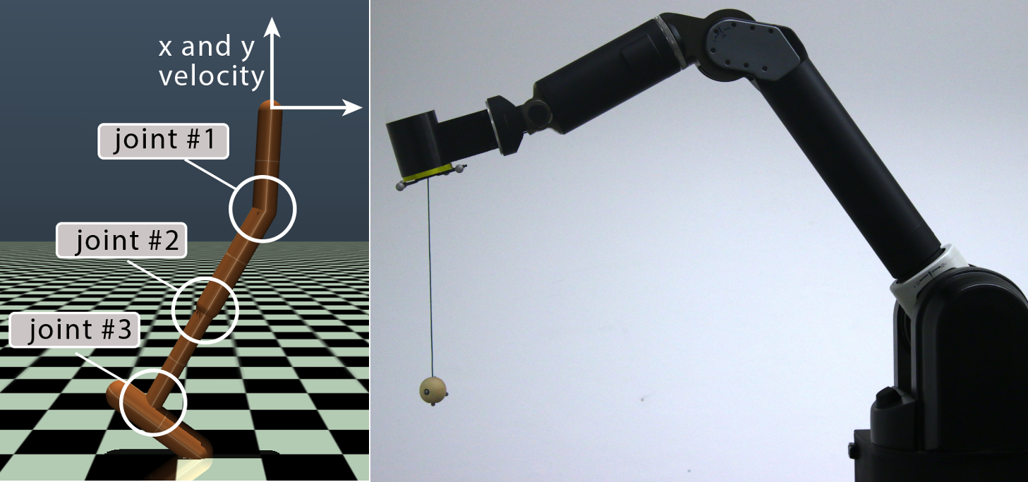
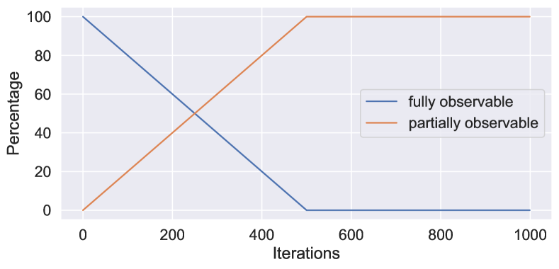
Figure 1: We propose a reinforcement learning approach called PO-GRL to optimize robot behavior under partial observability. (Bottom) PO-GRL transitions from full observability to partial observability during optimization allowing to utilize full state information but ending up with a policy assuming solely partial observability. We evaluate PO-GRL in both discrete and continuous simulation tasks and on a real robot. (Top Left) An example of a continuous simulation task where the robot can not observe the highlighted joints and x and y velocity. (Top Right) Barrett WAM performing the ball-in-the-cup task with a partially observed ball.

To make policy optimization more efficient we utilize full state information during training. In many robotic applications, training can be done in simulation with access to full state information, and, the optimized policy transferred to the real system. Even without (exact) simulation, physical systems can be set up to provide more information during training compared to running the final optimized policy. For example, in robotic multi-object manipulation with visual sensory input objects are partially observable [6]. However, the objects could be marked with markers during training to yield full state information. As another example, for hydraulic machines without proprioception one could attach markers to robot links for full state information during training. Similarly, mobile robots that rely on visual input for localization [7] could be trained by using preconfigured measuring posts.

To take a step closer to solving POMDPs we propose a simple but efficient approach that utilizes full state information during optimization. Classical work on RL under partial observability [8, 9, 10, 11] focuses on investigating different memory representations such as recurrent neural networks (RNNs) but does not consider how to make the learning process more efficient. Other methods are either application specific [12], utilize models [13, 14], or make the policy assume information which is not available during online operation [15, 16]. We focus on model-free RL that enables us to optimize policies directly through system interactions without learning a model. We propose a novel approach, called PO-GRL, which guides RL algorithms with additional full state information during the training phase. Our approach, illustrated in Fig. 1, is based on mixing full and partial state information while we gradually decrease the amount of full state information during training ending up with a policy compatible with partial observations. Our approach is able to efficiently learn behavior for fully observable parts without sacrificing performance in the partially observable parts of the problem.

II Related Work

The most naive strategy for dealing with partial observability is to ignore it. [17] treats observations as if they were states of the environment and Markov decision process (MDP) methods are applied to learn potentially sub-optimal behavior. So-called memory-based approaches use finite memory representations to learn based on previous interactions with the environment. Long Short-Term Memory (LSTM) has been studied widely as a memory representation [9, 18, 10, 11, 8]. Even with memory it is challenging to learn optimal behavior. [19] proposes a prediction constrained training for POMDPs which allows effective model learning even in the settings with misspecified models, as it can ignore observation patterns that would distract classic two-stage training. All these methods focus on memory representation rather than on the optimization of the policy itself. As an alternative for training an RNN to summarize the past, [20] learns a generative model of the environment and perform inference in this model to effectively aggregate the available information.

Guided RL approaches support RL algorithms during the learning process to increase their performance at test time. Guided policy search interleaves model-based trajectory optimization and deep learning for trajectory based tasks [13, 14, 21, 3, 22]. Guided policy search has been extended with continuous-valued internal memory [23] for partially observable tasks. [12] present an algorithm which combines model predictive control (MPC) with guided policy search in the special domain of quadcopters. The full state is known at training time when also MPC is used, but unavailable at test time. While all these guided policy search methods assume trajectory optimization with smooth trajectories, we focus on a more general setting and also evaluate our approach in benchmarks such as RockSample where trajectory optimization is not possible.

Regarding utilizing full state information when optimizing general RL policies under partial observability, [15] presents a guided actor-critic approach for learning policies for a set of cooperative homogeneous agents. While each actor learns a decentralized control policy operation on (partially observable) locally sensed information, the critic has access to the full system state. This means that the policy is optimized to assume full state information at each future time step. Such a policy cannot optimally consider information gathering under partial observability [17]. Similarly to [15], [16] proposes to use a guided actor-critic approach where the actor performs actions based on image input while the critic has access to full state information. Due to the critic being trained based on full state information the policy can be, similarly to [15], sub-optimal. Contrary to [15, 16] our optimization process starts by utilizing full state information but decreases the amount of full state information during optimization and ends up with a policy that has been adapted to the partially observable environment.

Finally, for completeness we mention that classic POMDP methods [24] assume a known model and typically discrete actions and observations. In contrast, we focus on model-free RL that can handle continuous actions and observations and directly learns from a reward signal.

III Preliminaries

This section discusses background information needed to understand our PO-GRL approach. First, we will describe the mathematical framework for POMDPs. Following standard notation [5, 25], a POMDP is a tuple $<\lx@glossaries@gls@link{symbol}{sspace}{\leavevmode\mathpzc{S}},\lx@glossaries@gls@link{symbol}{acspace}{\leavevmode\mathpzc{A}},\lx@glossaries@gls@link{symbol}{obspace}{\leavevmode\mathpzc{O}},P,\mathcal{O},r>$ consisting of states $\lx@glossaries@gls@link{symbol}{s}{\leavevmode\boldsymbol{\mathrm{s}}}\in\lx@glossaries@gls@link{symbol}{sspace}{\leavevmode\mathpzc{S}}$, actions $\lx@glossaries@gls@link{symbol}{ac}{\leavevmode\boldsymbol{\mathrm{a}}}\in\lx@glossaries@gls@link{symbol}{acspace}{\leavevmode\mathpzc{A}}$, and observations $\lx@glossaries@gls@link{symbol}{ob}{\leavevmode\boldsymbol{\mathrm{o}}}\in\lx@glossaries@gls@link{symbol}{obspace}{\leavevmode\mathpzc{O}}$. $P(\lx@glossaries@gls@link{symbol}{s}{\leavevmode\boldsymbol{\mathrm{s}}}^{\prime}|\lx@glossaries@gls@link{symbol}{s}{\leavevmode\boldsymbol{\mathrm{s}}},\lx@glossaries@gls@link{symbol}{ac}{\leavevmode\boldsymbol{\mathrm{a}}})$ is the probability (for continuous values a probability density) of ending in state $\lx@glossaries@gls@link{symbol}{s}{\leavevmode\boldsymbol{\mathrm{s}}}^{\prime}$ when starting in state s and executing action a. $\mathcal{O}(\lx@glossaries@gls@link{symbol}{ob}{\leavevmode\boldsymbol{\mathrm{o}}}|\lx@glossaries@gls@link{symbol}{s}{\leavevmode\boldsymbol{\mathrm{s}}}^{\prime},\lx@glossaries@gls@link{symbol}{ac}{\leavevmode\boldsymbol{\mathrm{a}}})$ is the probability of making observation o given that the agent took action a and landed in state $\lx@glossaries@gls@link{symbol}{s}{\leavevmode\boldsymbol{\mathrm{s}}}^{\prime}$. $r(\lx@glossaries@gls@link{symbol}{s}{\leavevmode\boldsymbol{\mathrm{s}}},\lx@glossaries@gls@link{symbol}{ac}{\leavevmode\boldsymbol{\mathrm{a}}})$ is the reward function.

As input for the underlaying algorithms, we maintain a history $\boldsymbol{\mathrm{h}}$ containing the last $H$ observations (and actions), where the horizon $H$ is an a-priori defined parameter. For further details see section V-A. The full history is a sufficient statistic for optimal decision making in POMDPs and a finite history an approximation [17]. The goal in RL for POMDPs is to find a policy $\pi(\lx@glossaries@gls@link{symbol}{ac}{\leavevmode\boldsymbol{\mathrm{a}}}_{t}|\lx@glossaries@gls@link{symbol}{h}{\leavevmode\boldsymbol{\mathrm{h}}}_{t})$ that maximizes the expected reward $\mathbb{E}_{\lx@glossaries@gls@link{symbol}{h}{\leavevmode\boldsymbol{\mathrm{h}}}_{0},\lx@glossaries@gls@link{symbol}{ac}{\leavevmode\boldsymbol{\mathrm{a}}}_{0},...}[\sum_{t=0}^{\infty}\gamma^{t}r(\lx@glossaries@gls@link{symbol}{h}{\leavevmode\boldsymbol{\mathrm{h}}}_{t},\lx@glossaries@gls@link{symbol}{ac}{\leavevmode\boldsymbol{\mathrm{a}}}_{t})]$. In the continuous case, the expected reward can be defined as [26]

$$J(\pi)=\iint p_{\pi}(\lx@glossaries@gls@link{symbol}{h}{\leavevmode\boldsymbol{\mathrm{h}}})\pi(\lx@glossaries@gls@link{symbol}{ac}{\leavevmode\boldsymbol{\mathrm{a}}}|\lx@glossaries@gls@link{symbol}{h}{\leavevmode\boldsymbol{\mathrm{h}}})Q^{\pi}(\lx@glossaries@gls@link{symbol}{h}{\leavevmode\boldsymbol{\mathrm{h}}},\lx@glossaries@gls@link{symbol}{ac}{\leavevmode\boldsymbol{\mathrm{a}}})d\lx@glossaries@gls@link{symbol}{h}{\leavevmode\boldsymbol{\mathrm{h}}}d\lx@glossaries@gls@link{symbol}{ac}{\leavevmode\boldsymbol{\mathrm{a}}},$$

where $p_{\pi}(\lx@glossaries@gls@link{symbol}{h}{\leavevmode\boldsymbol{\mathrm{h}}})$ denotes a (discounted) observation history distribution induced by policy $\pi$ and

$$\begin{split}Q^{\pi}(\lx@glossaries@gls@link{symbol}{h}{\leavevmode\boldsymbol{\mathrm{h}}}_{t},\lx@glossaries@gls@link{symbol}{ac}{\leavevmode\boldsymbol{\mathrm{a}}}_{t})&=\mathbb{E}_{\lx@glossaries@gls@link{symbol}{h}{\leavevmode\boldsymbol{\mathrm{h}}}_{t+1},\lx@glossaries@gls@link{symbol}{ac}{\leavevmode\boldsymbol{\mathrm{a}}}_{t+1},...}\Bigg{[}\sum_{t=0}^{\infty}\gamma^{t}r(\lx@glossaries@gls@link{symbol}{h}{\leavevmode\boldsymbol{\mathrm{h}}}_{t},\lx@glossaries@gls@link{symbol}{ac}{\leavevmode\boldsymbol{\mathrm{a}}}_{t})\Bigg{]},\\ V^{\pi}(\lx@glossaries@gls@link{symbol}{h}{\leavevmode\boldsymbol{\mathrm{h}}}_{t})&=\mathbb{E}_{\lx@glossaries@gls@link{symbol}{ac}{\leavevmode\boldsymbol{\mathrm{a}}}_{t},\lx@glossaries@gls@link{symbol}{h}{\leavevmode\boldsymbol{\mathrm{h}}}_{t+1},...}\Bigg{[}\sum_{t=0}^{\infty}\gamma^{t}r(\lx@glossaries@gls@link{symbol}{h}{\leavevmode\boldsymbol{\mathrm{h}}}_{t},\lx@glossaries@gls@link{symbol}{ac}{\leavevmode\boldsymbol{\mathrm{a}}}_{t})\Bigg{]},\\ A^{\pi}(\lx@glossaries@gls@link{symbol}{h}{\leavevmode\boldsymbol{\mathrm{h}}}_{t},\lx@glossaries@gls@link{symbol}{ac}{\leavevmode\boldsymbol{\mathrm{a}}}_{t})&=Q^{\pi}(\lx@glossaries@gls@link{symbol}{h}{\leavevmode\boldsymbol{\mathrm{h}}}_{t},\lx@glossaries@gls@link{symbol}{ac}{\leavevmode\boldsymbol{\mathrm{a}}}_{t})-V^{\pi}(\lx@glossaries@gls@link{symbol}{h}{\leavevmode\boldsymbol{\mathrm{h}}}_{t})\end{split}$$

denote the state-action (history-action in the POMDP case) value function $Q^{\pi}(\lx@glossaries@gls@link{symbol}{h}{\leavevmode\boldsymbol{\mathrm{h}}}_{t},\lx@glossaries@gls@link{symbol}{ac}{\leavevmode\boldsymbol{\mathrm{a}}}_{t})$, the value function $V^{\pi}(\lx@glossaries@gls@link{symbol}{h}{\leavevmode\boldsymbol{\mathrm{h}}}_{t})$ and the advantage function $A^{\pi}(\lx@glossaries@gls@link{symbol}{h}{\leavevmode\boldsymbol{\mathrm{h}}}_{t},\lx@glossaries@gls@link{symbol}{ac}{\leavevmode\boldsymbol{\mathrm{a}}}_{t})$. For the discrete case, integrals can be replaced by sums.

IV Reinforcement Learning using Guided Observability

This section presents our PO-GRL approach. During training PO-GRL mixes both full and partial information until a defined point (for example, half of training iterations) decreasing linearly the amount of full information. For the remaining training iterations (for example, final half of training iterations) PO-GRL uses only partial information resulting in a policy fully compatible with partial observations. We demonstrate the example usage with the policy search algorithm compatible policy search (COPOS) and the actor-critic algorithm Soft Actor-Critic (SAC). PO-GRL has the same convergence guarantees as applying the underlaying RL algorithm directly on partial observations due to the full conditioning on partial observations.

We assume having access to both full and partial observations during training and only to partial observations at test time. Partial observability at test time can mean that parts of the full state information are missing or noisy, or that the complete observations are noisy. Further, we assume training on a fixed number of samples. We also assume that we know the dimensions of the observation vector that will not be available, or noisy, during the test phase. For training outside simulation, that is, in the real-world, it is often straightforward to generate additional state information e.g. by adding additional sensors or cameras in robotic tasks. By deactivating parts of the observations at test time, we simulate practical scenarios like broken sensors or omitting sensors to save costs. For problems where the fully observable parts are not at all related to the best solution, PO-GRL may not help. However, when full state information helps in solving some parts of the task our PO-GRL approach may help underlying algorithms escape poor local optima through additional state information. We will now describe our approach based on samples $\tau$ consisting of tuples of observations $\boldsymbol{\mathrm{o}}$, actions $\boldsymbol{\mathrm{a}}$ and rewards r.

Algorithm Description

Algorithm 1 shows the PO-GRL approach for batch-based RL algorithms which we use as the guiding algorithm template. The following procedure will be performed at the learning phase: At the beginning of training, all samples $\tau$ contain fully observable state information. The amount of full state information decreases linearly until $N_{\textrm{MIX}}$ training iterations (see Algorithm 1, Lines 4 and 5). From that point the training will be continued with only partial information to optimize the final policy for partial observability (see Algorithm 1, Line 7). Fig. 1(Bottom) visualizes this general procedure. For simplicity, in the experiments we always mixed samples until reaching half of the iterations in the learning phase. For example, for 1000 training iterations the parameter $N_{\textrm{MIX}}$ will be set to 500. Interestingly, as shown in the experiments in section V the results are not sensitive to $N_{\textrm{MIX}}$. In the future, depending on the problem, parameter $N_{\textrm{MIX}}$ could be optionally fine-tuned. Now, we provide further implementation details for two types of algorithms: batch-based algorithms like COPOS, Trust Region Policy Optimization (TRPO) [26], or Proximal Policy Optimization (PPO) [27] and algorithms using a replay buffer like SAC.

Implementation Details for COPOS

Batch-based algorithms like COPOS use a sample set $\mathpzc{T}$, received from environment interactions in each iteration. Training in simulation, the environment returns always fully observable samples (Algorithm 1, Line 3). At training iteration $i$, when $i<N_{\textrm{MIX}}$, we directly make $|\mathpzc{T}|\cdot i/N_{\textrm{MIX}}$ samples partially observable (Algorithm 1, Line 5) (when $i\geq N_{\textrm{MIX}}$ we make all samples partially observable). For partially observable samples, we overwrite partially observable dimensions with zeros and set a flag. At test time the environment directly return partially observable observations. We implemented the COPOS algorithm for discrete and continuous action spaces as well as PO-GRL as a guided version of COPOS using the OpenAI baselines framework [28].

1:  Initialize $\pi_{0}$, $N_{\textrm{MIX}}$

2:  for i = 0 to max iterations - 1 do

3:     Generate sample set $\mathpzc{T}$ using $\pi_{i}$

4:     if $i<N_{\textrm{MIX}}$ then

5:        Make $|\mathpzc{T}|\cdot i/N_{\textrm{MIX}}$ samples partially observable

6:     else

7:        Make all samples partially observable

8:     end if

9:     Optimize and update $\pi_{i+1}$ using modified set $\mathpzc{T}$

10:  end for

Algorithm 1 Partially Observable Guided Reinforcement Learning (PO-GRL)

Implementation Details for SAC

Some algorithms like SAC have no explicit sampling phase to collect individual sample sets for the optimization, instead they perform the optimization based on a (fixed-length, rolling) replay buffer where samples are collected after each environment interaction. Training is performed on batches sampled from the replay buffer. To apply PO-GRL, we can modify these batches to contain $N_{\textrm{BATCH}}\cdot i/N_{\textrm{MIX}}$ partially observable samples for training iterations $i<N_{\textrm{MIX}}$, where $N_{\textrm{BATCH}}$ is the batch size, and for $i\geq N_{\textrm{MIX}}$ we use only partially observable samples. However, this modification of each batch can be computationally heavy. Therefore, in the experiments, before $N_{\textrm{MIX}}$ training iterations, we make a sample partially observable already before inserting it into the replay buffer. Samples are made partially observable according to the probability $n_{\textrm{CURRENT}}/n_{\textrm{MIX}}$, where $n_{\textrm{MIX}}$ is the total number of samples obtained in $N_{\textrm{MIX}}$ training iterations and $n_{\textrm{CURRENT}}$ is the index of the current sample. After $N_{\textrm{MIX}}$ training iterations we use only partially observable samples. Note, that for SAC, the replay buffer should not be too long, otherwise the optimization might still take fully observable samples into account long after the last fully observable sample was added to the buffer. In contrast, setting the replay buffer length too short, the performance of SAC will decrease significantly. We modified the implementation of the SAC algorithm from the Stable Baselines framework [29] using our PO-GRL approach.

V Experimental Results

Our experimental evaluation was designed to answer the following research questions:

1. How does our PO-GRL approach perform on POMDP problems compared to other model-free RL algorithms? Could our approach lead the policy search algorithm COPOS and actor-critic algorithm SAC to produce better results in contrast to learning only on partial state information?

2. Is our approach useful when the observations contain symmetric noise? How does the application of our approach affect the results in comparison to training directly on noisy observations?

To clarify the first question we analyzed the performance of our approach and other RL algorithms on different POMDP tasks. For answering the second question we designed a continuous control task where all observations returned by the environment are noisy. Also in this task, we compare our approach against training on either noisy or the original state information.

TABLE I: Mean of the average return (average discounted return on discrete tasks) on nine fully observable tasks over the last 40 episodes ± standard error over 50 random seeds.

Task (Timesteps)	COPOS	PPO	PPO-LSTM	SAC	TRPO
HalfCheetah-v2 (1M)	1629.53±69.91	1303.73±78.72	1460.23±70.58	3830.97±357.30	1009.25±27.33
Hopper-v2 (1M)	1899.34±81.80	1161.65±75.75	1587.66±58.28	2130.49±61.89	1647.12±38.42
InvertedDoublePendulum-v2 (1M)	8112.95±181.20	3367.50±208.42	3889.17±76.66	5164.28±266.02	6589.08±277.21
LunarLander-POMDP (5M)	233.07±1.29	26.06±13.94	122.58±39.07	240.06±0.61	204.45±3.52
Noisy-LunarLander (5M)	255.61±2.83	140.59±11.15	53.12±13.44	-	248.07±3.26
Reacher-v2 (1M)	-4.61±0.04	-6.37±0.13	-11.12±0.09	-6.86±0.09	-4.74±0.05
RockSample(4,4) (3M)	12.82±0.28	-	-	-	9.03±0.20
RockSample(5,7) (10M)	13.13±0.29	-	-	-	8.37±0.16
Swimmer-v2 (1M)	101.03±2.42	84.79±3.26	72.49±3.66	51.83±2.42	114.95±0.73
Walker2d-v2 (1M)	1147.71±89.68	871.69±44.40	1049.95±34.85	3740.61±78.33	1331.77±49.70

TABLE II: Mean of the average return (average discounted return on discrete tasks) on nine partially observable tasks over the last 40 episodes ± standard error over 50 random seeds.

Task (Timesteps)	COPOS	COPOS-guided	PPO	PPO-LSTM
HalfCheetah-v2 (1M)	1490.79±48.58	1491.02±59.99	1314.10±59.97	1157.11±44.12
Hopper-v2 (1M)	1411.96±77.40	2219.61±83.34	994.93 ±48.56	955.15±33.31
InvertedDoublePendulum-v2 (1M)	5528.74±297.16	7535.25±241.52	2629.53±133.94	935,93±21.89
LunarLander-POMDP (5M)	81.03±20.29	154.16±15.03	-195.06±17.99	-272.95±37.26
Noisy-LunarLander (10M)	124.34±1.76	132.74±2.32	-153.24±12.89	-117.54±7.19
Reacher-v2 (1M)	-9.35±0.05	-4.69±0.05	-9.66±0.05	-14.01±0.06
RockSample(4,4) (3M)	9.95±0.28	11.83±0.30	-	-
RockSample(5,7) (10M)	8.07±0.02	9.66±0.21	-	-
Swimmer-v2 (1M)	60.95±2.09	92.63±2.96	38.04±1.30	35.82±0.45
Walker2d-v2 (1M)	780.44±46.69	993.29±78.10	598.23±18.06	699.56±10.53

Task (Timesteps)	SAC	SAC-guided	TRPO
HalfCheetah-v2 (1M)	1536.54±119.12	1835.62±154.52	1049.87±31.06
Hopper-v2 (1M)	726.70±37.76	858.00±55.88	1038.55±12.95
InvertedDoublePendulum-v2 (1M)	6661.90±161.32	5922.65±252.54	5089.96±190.03
LunarLander-POMDP (5M)	-70.13±11.17	-	-52.43±15.86
Noisy-LunarLander (10M)	-	-	123.00±2.47
Reacher-v2 (1M)	-11.06±0.20	-11.58±0.24	-9.34±0.06
RockSample(4,4) (3M)	-	-	8.57±0.25
RockSample(5,7) (10M)	-	-	8.15±0.00
Swimmer-v2 (1M)	41.47±0.77	42.25±0.68	67.67±1.19
Walker2d-v2 (1M)	1892.36±88.80	1911.40±99.52	862.46±27.01

V-A Experimental Setup

For continuous action space experiments, we evaluate LunarLander-POMDP [30], Noisy-LunarLander and six tasks in the MuJoCo [31] physics simulator. The LunarLander-POMDP environment is a modification that turns the OpenAI Gym [32] environment LunarLanderContinuous-v2 into a partially observable problem by adding a ”blind” area between the starting point on the top and the landing pad. Inside the the blind area the lander agent cannot perceive any information of the environment. Instead of using the original observation output from the environment, we use a history of fixed length as input for the RL algorithms which is more suitable for solving POMDPs. The history includes the last $H$ observations $\boldsymbol{\mathrm{o}}$, actions $\boldsymbol{\mathrm{a}}$ and a flag $f$ that tells the algorithm whether full or partial state information is available. We define the used history for time step $t$ as $\boldsymbol{h}_{t}=\big{(}f_{t},\lx@glossaries@gls@link{symbol}{ob}{\leavevmode\boldsymbol{\mathrm{o}}}_{t},\lx@glossaries@gls@link{symbol}{ac}{\leavevmode\boldsymbol{\mathrm{a}}}_{t-1},...,f_{t-H},\lx@glossaries@gls@link{symbol}{ob}{\leavevmode\boldsymbol{\mathrm{o}}}_{t-H},\lx@glossaries@gls@link{symbol}{ac}{\leavevmode\boldsymbol{\mathrm{a}}}_{t-H-1}\big{)}$. The history structure and the structure of the neural networks remain always the same in all three cases (fully observable, partially observable, guided) which enables us to focus on the differences between partial and full observability. Based on the LunarLanderContinuous-v2 environment we built another modification, called Noisy-LunarLander, to answer the second research question posed at the beginning of the section. We added Gaussian noise by randomly drawing samples from a normal (Gaussian) distribution, represented by the mean $\mu$ and the standard deviation $\sigma$. Additionally, we focus on the two-dimensional tasks HalfCheetah-v2, Hopper-v2, InvertedDoublePendulum-v2, Reacher-v2, Swimmer-v2 and Walker2d-v2 from MuJoCo. In order to create partially observable environments, we modified the MuJoCo tasks listed above by deactivating parts of the observation. Specifically, we select a number of dimensions of the observation vector and overwrite them with zeros. For the selection of these dimensions for the individual MuJoCo tasks, we run some preliminary tests and chose dimensions whose deactivation has a noticeable impact on the overall performance. Fig. 1(Top Left) visualizes these dimensions for Hopper-v2.

As the discrete action task, we use RockSample, a well-known benchmark problem for POMDP algorithms which was first introduced in [33]. We use the RockSample implementation from gym-pomdp [34] which are extensions of OpenAI Gym for POMDPs and built a wrapper which returns a history containing the following information: The agent’s observation for sampling or checking rocks, the position of the agent in the grid, the previously taken action and a flag that tells whether full or partial state information is available. In the fully observable case, the true rock values are additionally available. For our experiments, we use two different sizes of the problem: RockSample(4,4) and RockSample(5,7).

For each experimental run, we used one core on an Intel^® Xeon^® E5-2670 processor and a maximum of 6 GB RAM. We denote the guided versions of the COPOS and SAC algorithms ”COPOS-guided” and ”SAC-guided”, respectively. We compared against COPOS, SAC, TRPO, and PPO, where TRPO and PPO used the OpenAI baselines [28] implementation. Additionally, to test whether a different memory representation influences performance, we compared against PPO + LSTM [35] called ”PPO-LSTM” and implemented using Stable Baselines [29]. In preliminary experiments we also tried the OpenAI baselines implementation of PPO + LSTM but achieved better results with Stable Baselines. We ran all experiments for 50 random seeds each. For training, we used 1 million time steps in the MuJoCo tasks, 5 million time steps in LunarLander-POMDP, 10 million time steps in the Noisy-LunarLander environment, 3 million time steps in the RockSample(4,4) environment and 10 million time steps in the RockSample(5,7) environment. The performance in the first 50% timesteps for COPOS-guided and SAC-guided is evaluated on a mixture of fully and partially observable samples. The second half of iterations is evaluated on only partially observable samples.

V-B Results

Table II summarizes the results on all partially observable tasks targeting the first research question. We also ran all experiments in the fully observable case as baseline, see Table I. In the LunarLander-POMDP environment, we compared COPOS-guided with the algorithms COPOS, PPO, PPO-LSTM, SAC, and TRPO and rendered some runs of the LunarLander-POMDP (partially observable) environment with the final learned policy for COPOS-guided (see Figure 2(b)) and COPOS (see Figure 2(a)). There is a noticeable difference in learned behavior: With the policy learned by COPOS, the lander moves slowly into the blind area, then it falls fast through the blind area and after that slows down before landing, while with the policy learned by COPOS-guided, the speed of the lander is more constant also inside the blind area. Additionally, with COPOS-guided the lander does not turn off the orientation engine in the blind area as is done by COPOS in Figure 2(a).

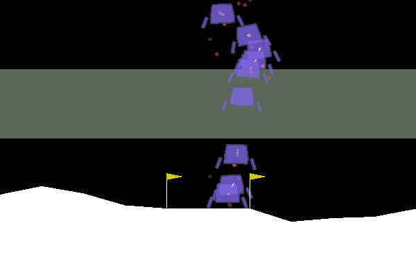
(a) Lander is heavily breaking
before blind area and falling through.

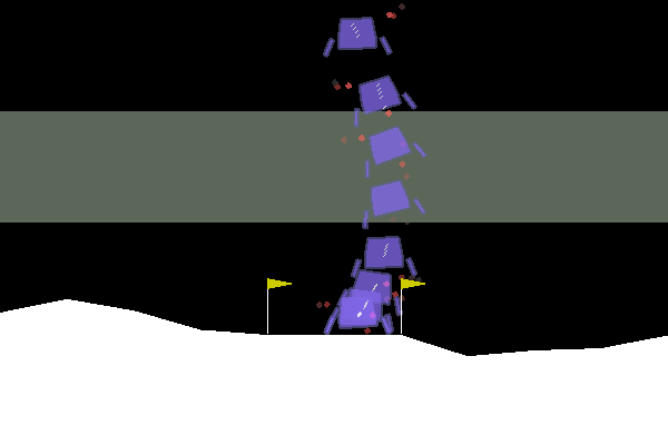
(b) Speed of the lander is constant also inside blind area.

Figure 2: Visualization of two trained policies in LunarLander-POMDP, where (a) is trained on partial information (COPOS) and (b) is trained with guided approach (COPOS-guided).

We compared COPOS-guided and SAC-guided to COPOS, PPO, PPO-LSTM, SAC, and TRPO, on six different continuous control tasks in the MuJoCo physics simulator. Table II shows that our PO-GRL approach, meaning either COPOS-guided or SAC-guided, improves the performance in all partially observable MuJoCo tasks.

For evaluating our PO-GRL approach on environments with a discrete action space, we compared COPOS-guided against COPOS and TRPO. We were not able to test against SAC because this algorithm is only implemented for continuous action spaces. Table II demonstrates that COPOS-guided outperformed the other algorithms in both problem sizes (for more details, see Figure 1 in the supplement). Our approach supports the algorithm not being stuck in poor local optima and therefore allows to learn a more advanced policy. RockSample is a challenging task for model-free approaches because there is no learned model of the environment including the position of the rocks available. Therefore, approaches which require an exact model already achieve better results on this problem. For example, Heuristic Search Value Iteration (HSVI) [33] achieves a reward of $18.0$ on RockSample(4,4) and a reward of $23.1$ on RockSample(5,7).

To investigate our second research question, we compared COPOS-guided against COPOS, PPO, PPO-LSTM and TRPO in our Noisy-LunarLander environment. For the Gaussian noise we use the parameters $\mu=0$ and $\sigma=0.3$. Table II shows that the PO-GRL approach leads to a higher performance than using COPOS, PPO, PPO-LSTM or TRPO directly on noisy data.

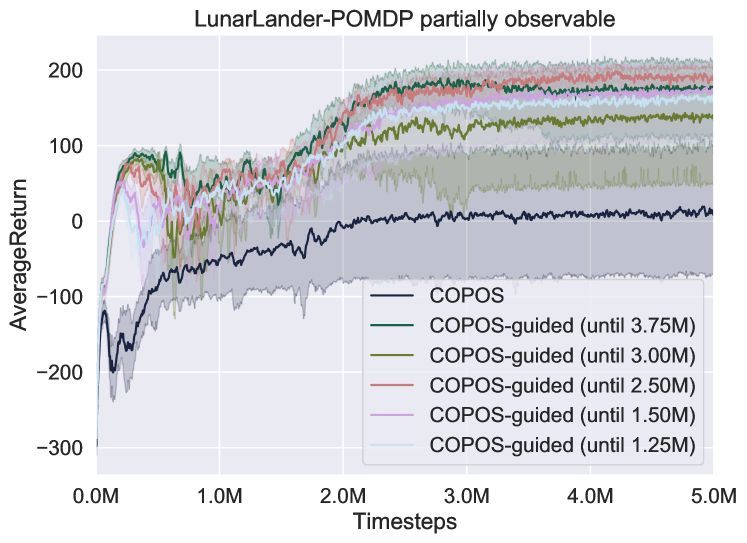
Figure 3: Average return for different mixing rates on LunarLander-POMDP with partial observations over 10 random seeds. In the legend, value in parenthesis indicates when mixing full and partial observations stops and purely partial observations are used. Algorithms were executed for 5 million time steps. Shaded area denotes the bootstrapped 95% confidence interval.

Since the same mixing rate schedule of full and partial observations worked in all the tasks our approach does not appear to be sensitive to the mixing rate. To test the sensitivity to the mixing rate schedules even further, we ran an additional experiment for COPOS-guided with different schedules in LunarLander-POMDP as shown in Figure 3. For all schedules COPOS-guided outperformed COPOS.

VI Real-Robot Experiment

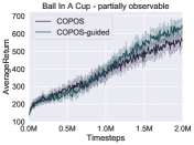
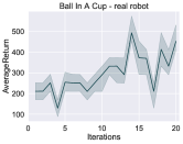
Figure 4: Results for the ball-in-a-cup task using the Barrett WAM robot arm. The left plot shows the average return for COPOS and COPOS-guided in simulation runs. The right plot shows the average return obtained when continuing training of COPOS-guided on the real robot as well as the $0.25$ and $0.75$ computed via bootstrap sampling.

To validate our method in a real-world sim2real scenario, we applied PO-GRL using COPOS to a ball in a cup task shown in Fig. 1 (top right). In the task a robot with a WAM arm from Barrett Technologies tries to swing the ball hanging from a string into a cup. In our setup, the actions of the RL agent are the displacements of the desired joint positions that are then tracked by the low-level controller of the robot. The agent controls only three of the seven degrees of freedom of the robot, as the remaining DoFs are not necessary to learn the task. As can be seen in Fig. 1 (top right), both ball and cup are equipped with OptiTrack markers that allows to reliably estimate the position of the ball and the cup. This allows to compute the reward function on the real system and generate observations for the RL agent, which consist of current joint position and velocity of the robot, desired joint position as well as the position of the ball. Under partial observability the velocity of the ball is not observed and at each time step we freeze the pall position with $5$% probability for 5 consecutive frames. We first train the policy using COPOS and COPOS-guided in a simulator for $2$M time steps. Since COPOS-guided outperformed COPOS in simulation as shown in Fig. 4 (left) we continued with COPOS-guided for another $20$ iterations on the real robot, where in each iteration $20$ episodes are performed. As shown in Fig. 4 (right), this learning step on the real system increased the average reward from $210$ to $452$. Finally, we executed both the learned policy before and after training on the real robot using $40$ episodes in order to gain an impression of the qualitative performance of the policies. We observed, that training on the real robot improved the success rate of the policy from $17.5\%$ to $45\%$, underlining the potential of exploiting state-information during training in simulation with a subsequent training step in reality.

VII Conclusion

In this work, we proposed PO-GRL which guides RL algorithms with additional full state information during training to increase the performance in the test phase. PO-GRL produces a policy which does not rely on assumptions about state information in the test phase. During training PO-GRL mixes samples with both full and partial state information, starting with full observability but ending with a policy needing only partial observations. The simple formulation allows applying the approach to a variety of RL methods. Further, we are able to efficiently learn behavior for parts of the problem that are actually fully observable while making learning easier for the algorithms due to using full observability at the beginning of learning. In the experiments, PO-GRL outperformed baseline algorithms trained directly on partial observations in different continuous and discrete tasks. As a history representation needed in POMDP tasks we used a simple windowing approach in form of a fixed-length history. In future work it would be interesting to replace this representation with an LSTM to be able to memorize events over a very long horizon. Our approach mixes fully and partially observable samples linearly. At this point there is also potential for future work by applying more complex functions for the ratio between fully and partially observable samples at the beginning of training.

Supplementary Material

VIII Additional Plots for Experiments

Figure 5 shows performance plots for two instances of the RockSample problem and Figure 6 shows the performance and entropy plots for the Noisy-LunarLander task. Additional entropy plots can be found in Figure 7 and Figure 8.

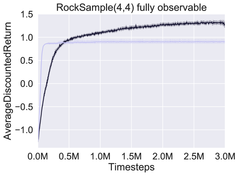
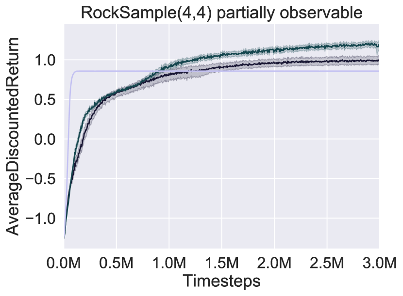
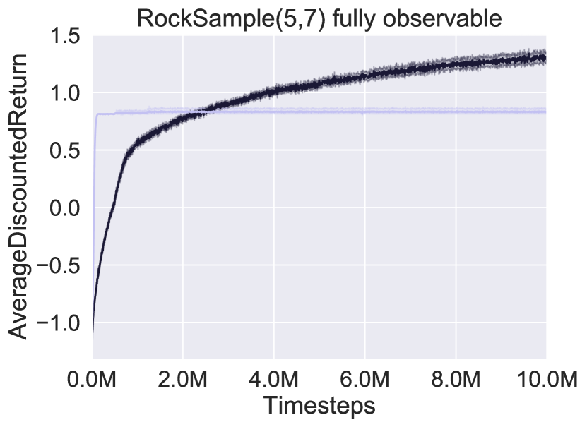
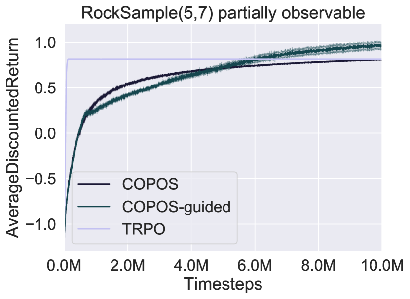
Figure 5: Average discounted return for two instances of RockSample, both with full observations (left) and partial observations (right) over 50 random seeds. Algorithms were executed for 5 million time steps on RockSample(4,4) (top) and 10 million time steps on RockSample(5,7) (bottom). Shaded area denotes the bootstrapped 95% confidence interval.

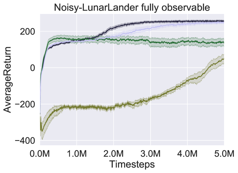
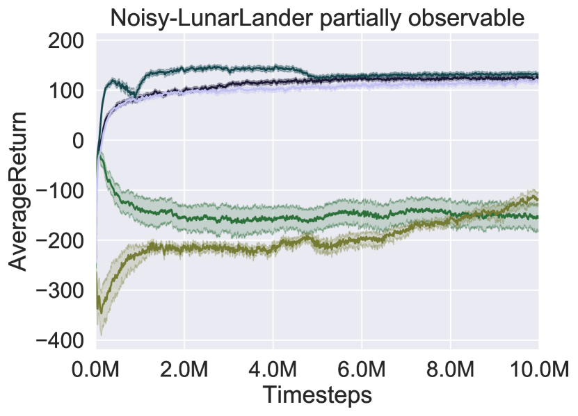
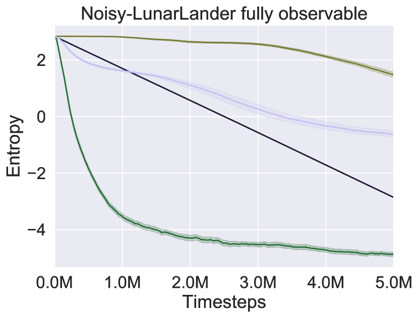
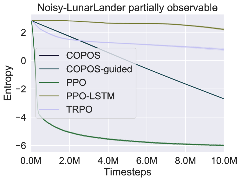
Figure 6: Average return (top) and entropy (bottom) for both Noisy-LunarLander with full observations (left) and noisy observations (right) over 50 random seeds. Algorithms were executed for 10 million time steps (5 million time steps in the fully observable case). Shaded area denotes the bootstrapped 95% confidence interval.

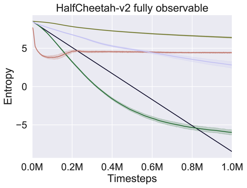
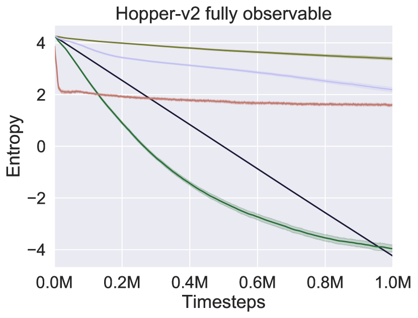
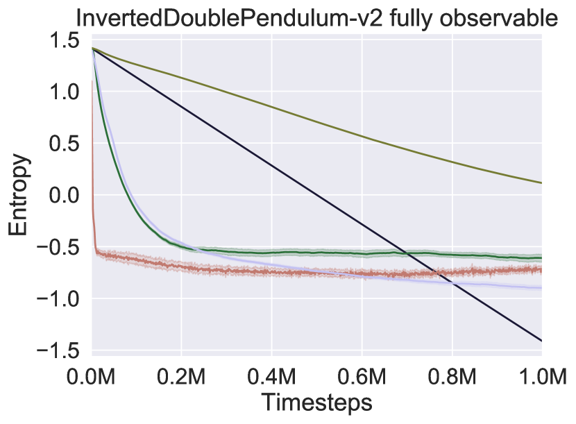
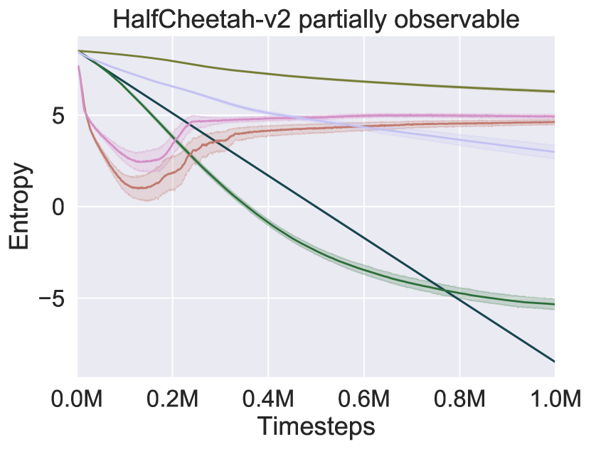
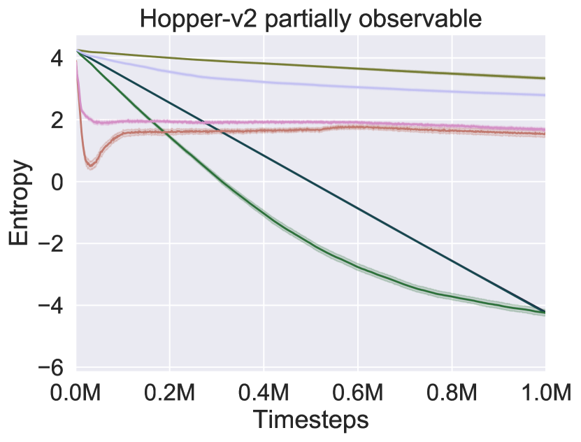
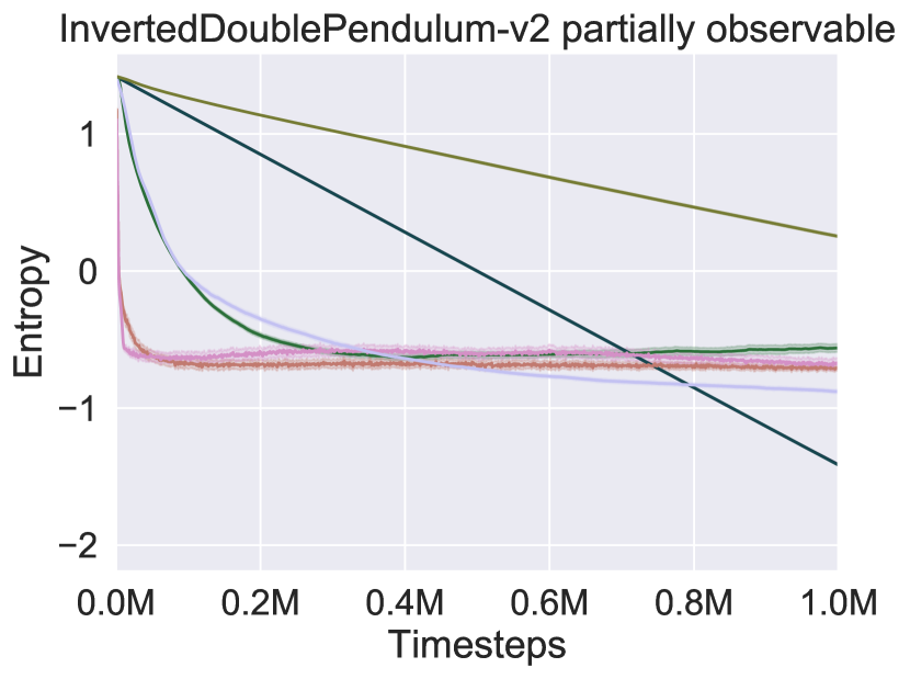
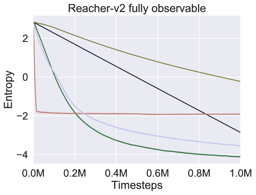
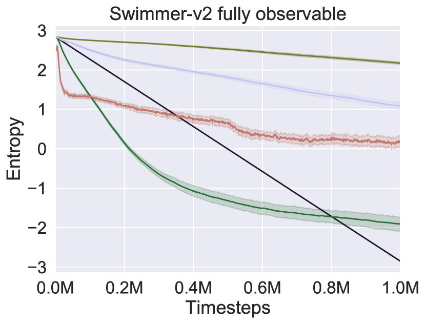
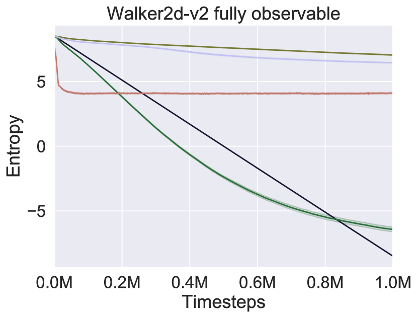
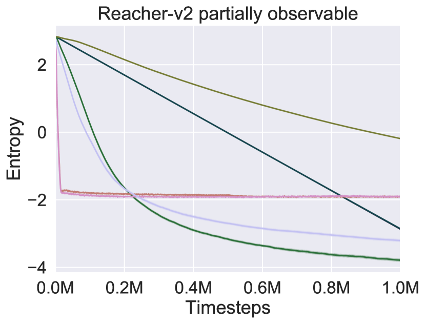
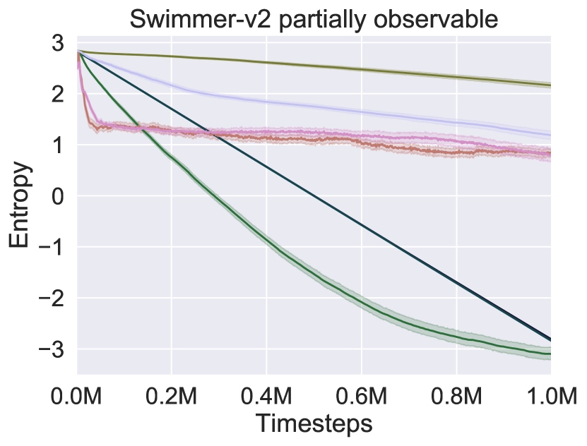
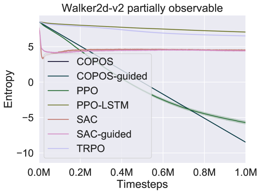
Figure 7: Entropy for MuJoCo tasks over 50 random seeds. Algorithms were executed for 1 million time steps. Shaded area denotes the bootstrapped 95% confidence interval.

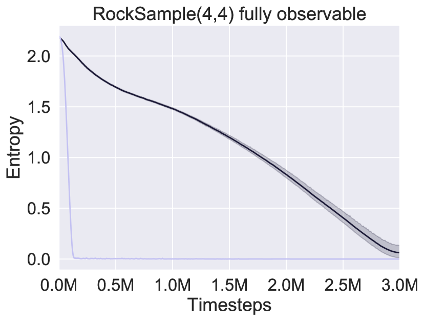
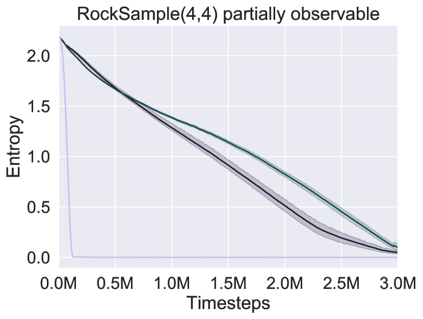
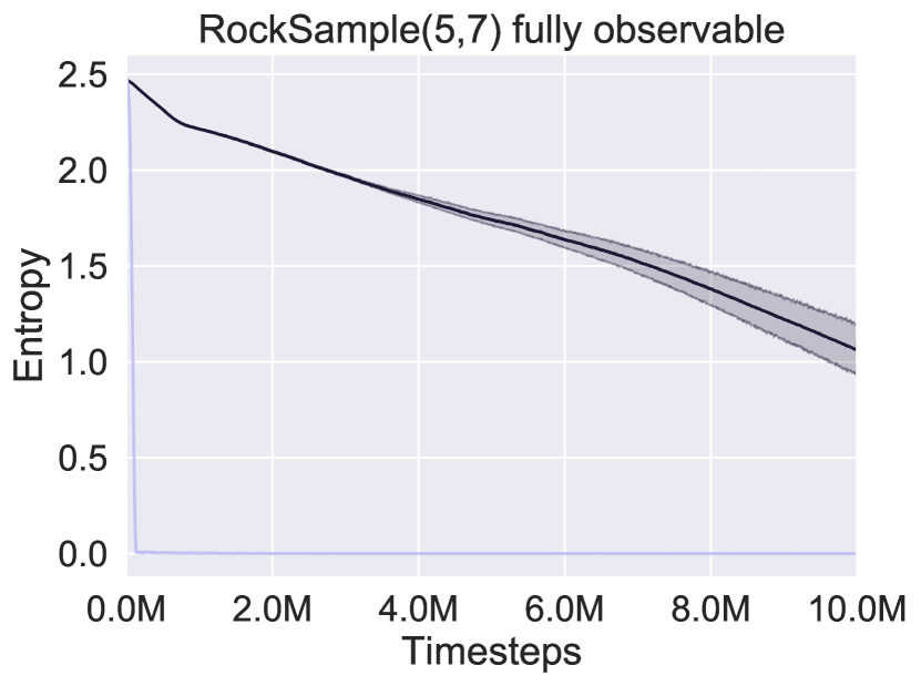
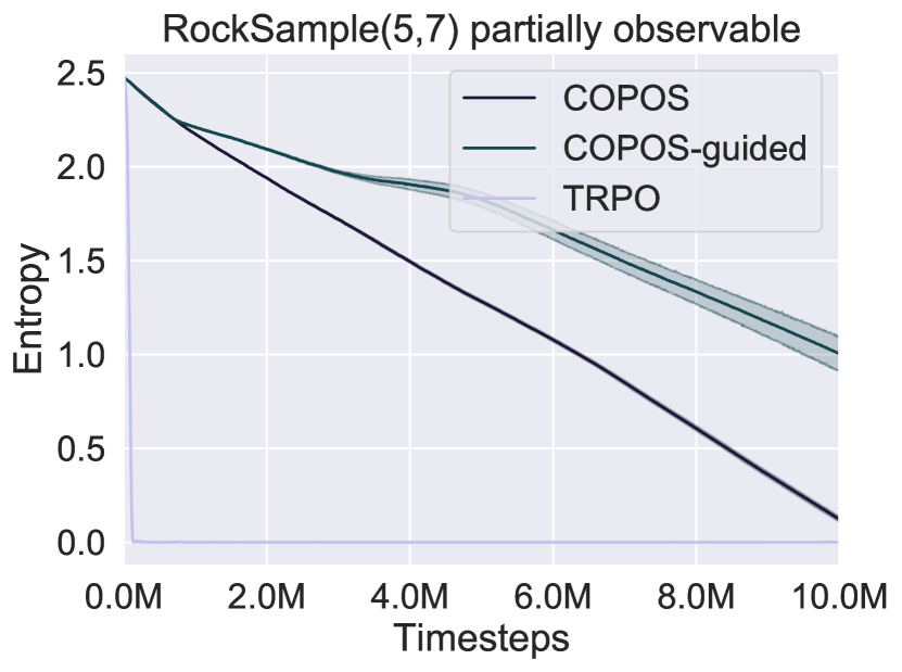
Figure 8: Entropy for two instances of RockSample, both with full observations (left) and partial observations (right) over 50 random seeds. Algorithms were executed for 5 million time steps on RockSample(4,4) (top) and 10 million time steps on RockSample(5,7) (bottom). Shaded area denotes the bootstrapped 95% confidence interval.

IX MuJoCo POMDP tasks

See Table III for a detailed overview of MuJoCo tasks that we modified into partially observable tasks by deactivation some dimensions of the observations vector.

TABLE III: Observation (Ob.) space dimensionality and the dimensions we deactivated for the partially observable versions of the MuJoCo tasks. The column ”Description” is for the inactive observation dimensions in the POMDP versions.

Task	Ob. Space	Inactive Ob.	Description
	Dim.	Dim.
HalfCheetah-v2	17	3-10	angle of front/back thigh, shin and foot joint
			x and y velocity
Hopper-v2	11	3-7	angle of thigh, leg and foot joint
			x and y velocity
InvertedDoublePend.-v2	11	1-4	angle of both pole joints
			y position of both pole joints
Reacher-v2	11	5-11	target x and y position
			angular velocity of both joints
			distance between fingertip and target
Swimmer-v2	8	2-6	angle of both joints, x and y velocity
			angular velocity of torso
Walker2d-v2	17	9-14	x and y velocity, angular velocity of torso
			angular velocity of right thigh, shin and foot joint

X Experiment Parameters

Additionally to the parameters already described in section 5.1, see Table IV for COPOS, Table V for PPO, Table VI for PPO-LSTM, Table VII for SAC and Table VIII for TRPO.

TABLE IV: Hyperparameters for running the COPOS algorithm.

Parameter	Value
Number of hidden neural network layers	2
Units per hidden layer	32
Hidden activation function	tanh
Time steps per batch	5000 (LunarLander and RockSample) or 2000 (MuJoCo)
Maximum KL-divergence ($\beta$)	0.01
Maximum difference in entropy ($\epsilon$)	auto (continuous tasks) or 0.01 (discrete tasks)
Conjugate gradient iterations	10
Conjugate gradient damping	0.1
GAE parameters ($\gamma$ and $\lambda$)	0.99 and 0.98
Value function iterations	5
Value function step size	0.001

TABLE V: Hyperparameters for running the PPO algorithm.

Parameter	Value
Number of hidden neural network layers	2
Units per hidden layer	64
Hidden activation function	tanh
Time steps per batch	2048
Number of mini-batches	32
Clip range	0.2
GAE parameters ($\gamma$ and $\lambda$)	0.99 and 0.95
Number of epochs	10
Learning rate	$3\cdot 10^{-4}$

TABLE VI: Hyperparameters for running the PPO-LSTM algorithm.

Parameter	Value
LSTM network size	32
Activation function	tanh
Time steps per batch	2048
Number of mini-batches	1
Clip range	0.2
GAE parameters ($\gamma$ and $\lambda$)	0.99 and 0.95
Number of epochs	10
Learning rate	$3\cdot 10^{-4}$

TABLE VII: Hyperparameters for running the SAC algorithm.

Parameter	Value
Number of hidden neural network layers	2
Units per hidden layer	256
Hidden activation function	ReLU
Batchsize	256
Target update interval	1
Gradient steps	1
Buffer size	$5\cdot 10^{5}$
Learning rate	$3\cdot 10^{-4}$

TABLE VIII: Hyperparameters for running the TRPO algorithm.

Parameter	Value
Number of hidden neural network layers	2
Units per hidden layer	32
Hidden activation function	tanh
Time steps per batch	5000 (LunarLander and RockSample) or 2000 (MuJoCo)
Maximum KL-divergence	0.01
Conjugate gradient iterations	10
Conjugate gradient damping	0.1
GAE parameters ($\gamma$ and $\lambda$)	0.99 and 0.98
Value function iterations	5
Value function step size	0.001

References

- [1] D. Silver, J. Schrittwieser, K. Simonyan, I. Antonoglou, A. Huang, A. Guez, T. Hubert, L. Baker, M. Lai, A. Bolton, et al., “Mastering the game of go without human knowledge,” Nature, vol. 550, no. 7676, p. 354, 2017.
- [2] O. Vinyals, I. Babuschkin, W. M. Czarnecki, M. Mathieu, A. Dudzik, J. Chung, D. H. Choi, R. Powell, T. Ewalds, P. Georgiev, et al., “Grandmaster level in starcraft ii using multi-agent reinforcement learning,” Nature, vol. 575, no. 7782, pp. 350–354, 2019.
- [3] S. Levine, C. Finn, T. Darrell, and P. Abbeel, “End-to-end training of deep visuomotor policies,” Journal of Machine Learning Research, vol. 17, no. 1, pp. 1334–1373, 2016.
- [4] S. Levine, P. Pastor, A. Krizhevsky, J. Ibarz, and D. Quillen, “Learning hand-eye coordination for robotic grasping with deep learning and large-scale data collection,” The International Journal of Robotics Research, vol. 37, no. 4-5, pp. 421–436, 2018.
- [5] L. P. Kaelbling, M. L. Littman, and A. R. Cassandra, “Planning and acting in partially observable stochastic domains,” Artificial intelligence, vol. 101, no. 1-2, pp. 99–134, 1998.
- [6] J. Pajarinen and V. Kyrki, “Robotic manipulation of multiple objects as a POMDP,” Artificial Intelligence, vol. 247, pp. 213–228, 2017.
- [7] N. Radwan, A. Valada, and W. Burgard, “Vlocnet++: Deep multitask learning for semantic visual localization and odometry,” IEEE Robotics and Automation Letters, vol. 3, no. 4, pp. 4407–4414, 2018.
- [8] B. Bakker, “Reinforcement learning with long short-term memory,” in Advances in neural information processing systems, 2002, pp. 1475–1482.
- [9] D. Wierstra, A. Foerster, J. Peters, and J. Schmidhuber, “Solving deep memory pomdps with recurrent policy gradients,” in International Conference on Artificial Neural Networks. Springer, 2007, pp. 697–706.
- [10] M. Hausknecht and P. Stone, “Deep recurrent q-learning for partially observable mdps,” in 2015 AAAI Fall Symposium Series, 2015.
- [11] N. Heess, J. J. Hunt, T. P. Lillicrap, and D. Silver, “Memory-based control with recurrent neural networks,” arXiv preprint arXiv:1512.04455, 2015.
- [12] T. Zhang, G. Kahn, S. Levine, and P. Abbeel, “Learning deep control policies for autonomous aerial vehicles with mpc-guided policy search,” in IEEE International Conference on Robotics and Automation (ICRA). IEEE, 2016, pp. 528–535.
- [13] S. Levine and V. Koltun, “Guided policy search,” in International Conference on Machine Learning, 2013, pp. 1–9.
- [14] ——, “Learning complex neural network policies with trajectory optimization,” in International Conference on Machine Learning, 2014, pp. 829–837.
- [15] M. Hüttenrauch, A. Šošić, and G. Neumann, “Guided deep reinforcement learning for swarm systems,” 2017.
- [16] L. Pinto, M. Andrychowicz, P. Welinder, W. Zaremba, and P. Abbeel, “Asymmetric actor critic for image-based robot learning,” in Proceedings of Robotics: Science and Systems, Pittsburgh, Pennsylvania, June 2018.
- [17] L. P. Kaelbling, M. L. Littman, and A. W. Moore, “Reinforcement learning: A survey,” Journal of artificial intelligence research, vol. 4, pp. 237–285, 1996.
- [18] D. Wierstra and J. Schmidhuber, “Policy gradient critics,” in European Conference on Machine Learning. Springer, 2007, pp. 466–477.
- [19] J. Futoma, S. Harvard, M. C. Hughes, and F. Doshi-Velez, “Prediction-constrained pomdps,” 32nd Conference on Neural Information Processing Systems (NIPS), 2018.
- [20] M. Igl, L. Zintgraf, T. A. Le, F. Wood, and S. Whiteson, “Deep variational reinforcement learning for POMDPs,” in International Conference on Machine Learning, 2018, pp. 2122–2131.
- [21] S. Levine, N. Wagener, and P. Abbeel, “Learning contact-rich manipulation skills with guided policy search (2015),” arXiv preprint arXiv:1501.05611, 2015.
- [22] W. H. Montgomery and S. Levine, “Guided policy search via approximate mirror descent,” in Advances in Neural Information Processing Systems, 2016, pp. 4008–4016.
- [23] M. Zhang, Z. McCarthy, C. Finn, S. Levine, and P. Abbeel, “Learning deep neural network policies with continuous memory states,” in 2016 IEEE International Conference on Robotics and Automation (ICRA). IEEE, 2016, pp. 520–527.
- [24] G. Shani, J. Pineau, and R. Kaplow, “A survey of point-based POMDP solvers,” Autonomous Agents and Multi-Agent Systems, vol. 27, no. 1, pp. 1–51, 2013.
- [25] M. Wiering and M. Van Otterlo, “Reinforcement learning,” Adaptation, learning, and optimization, vol. 12, p. 3, 2012.
- [26] J. Schulman, S. Levine, P. Abbeel, M. Jordan, and P. Moritz, “Trust region policy optimization,” in International conference on machine learning, 2015, pp. 1889–1897.
- [27] J. Schulman, F. Wolski, P. Dhariwal, A. Radford, and O. Klimov, “Proximal policy optimization algorithms,” arXiv preprint arXiv:1707.06347, 2017.
- [28] P. Dhariwal, C. Hesse, O. Klimov, A. Nichol, M. Plappert, A. Radford, J. Schulman, S. Sidor, Y. Wu, and P. Zhokhov, “Openai baselines,” https://github.com/openai/baselines, 2017.
- [29] A. Hill, A. Raffin, M. Ernestus, A. Gleave, R. Traore, P. Dhariwal, C. Hesse, O. Klimov, A. Nichol, M. Plappert, A. Radford, J. Schulman, S. Sidor, and Y. Wu, “Stable baselines,” https://github.com/hill-a/stable-baselines, 2018.
- [30] R. Zhi, “Deep reinforcement learning under uncertainty for autonomous driving,” Master’s thesis, Technische Universität Darmstadt, 2018.
- [31] E. Todorov, T. Erez, and Y. Tassa, “Mujoco: A physics engine for model-based control,” in 2012 IEEE/RSJ International Conference on Intelligent Robots and Systems. IEEE, 2012, pp. 5026–5033.
- [32] G. Brockman, V. Cheung, L. Pettersson, J. Schneider, J. Schulman, J. Tang, and W. Zaremba, “Openai gym,” 2016.
- [33] T. Smith and R. Simmons, “Heuristic search value iteration for pomdps,” in Proceedings of the 20th conference on Uncertainty in artificial intelligence. AUAI Press, 2004, pp. 520–527.
- [34] S. Totaro, “gym-pomdp,” https://github.com/d3sm0/gym˙pomdp, 2018.
- [35] S. Hochreiter and J. Schmidhuber, “Long short-term memory,” Neural computation, vol. 9, no. 8, pp. 1735–1780, 1997.