A Probabilistic Assessment of the COVID-19 Lockdown on Air Quality in the UK

Abstract

In March 2020 the United Kingdom (UK) entered a nationwide lockdown period due to the Covid-19 pandemic. As a result, levels of NO₂ in the atmosphere dropped. In this work, we use over 550,134 NO₂ data points from 237 stations in the UK to build a spatiotemporal Gaussian process (GP) capable of predicting NO₂ levels across the entire UK. We integrate several covariate datasets to enhance the model’s ability to capture the complex spatiotemporal dynamics of NO₂. Our numerical analyses show that, within two weeks of a UK lockdown being imposed, UK NO₂ levels dropped 36.8%. Further, we show that as a direct result of lockdown NO₂ levels were 29-38% lower than what they would have been had no lockdown occurred. In accompaniment to these numerical results, we provide a software framework that allows practitioners to easily and efficiently fit similar models.

1 Introduction

In response to the COVID-19 pandemic, many countries resorted to ordering citizens to remain at home. These lockdown measures had the effect of curtailing certain polluting activities, resulting in reduced pollutant concentrations in many places around the world (e.g. Forster et al.,, 2020). Clear evidence of reductions has been found in nitrogen dioxide (NO₂), a pollutant that can negatively impact respiratory health (Henschel and Chan,, 2013; Anenberg et al.,, 2018) and which is strongly associated with transport emissions due to the burning of fossil fuels (Sundvor et al.,, 2013). Yet these (often provisional) assessments of lockdown impacts on NO₂ have largely been restricted to analyses of individual measurement locations or satellite retrievals and focused on daily means (Berman and Ebisu,, 2020; Carslaw,, 2020; Schindler,, 2020), rather than combining information across different sources. In this paper we utilise a spatiotemporal approach to model the patterns of change in NO₂.

Modelling continuous spatiotemporal surfaces using a set of discrete observations is a common task in geostatistics (Diggle and Ribeiro,, 2007). This approach assumes that there exists a latent partially observed function which is commonly modelled with a GP. Consequently, it is then possible to construct a fully-Bayesian model. Historically these models have been computationally challenging due to their $\mathcal{O}(n^{3})$ cost, where $n$ is the number of datapoints. However, recent advances in the sparse GP literature has reduced this cost to $\mathcal{O}(nm^{2})$, where $m<<n$ (Hensman et al.,, 2013).

In this work we combine several measurement datasets and covariate information to build a highly informative spatiotemporal model that yields novel insights into the affect of the COVID-19 UK lockdown on NO₂ levels. To build a model that can be both computationally efficient to fit and powerful enough to capture the complex latent process, we use recent developments in the GP literature by using the SteinGP presented by Pinder et al., (2020). Finally, we examine the inferred latent function to report two quantitative results concerning the change in NO₂ levels. The first gives the integrated NO₂ levels pre and post-lockdown, and the second compares the latent function post-lockdown to the NO₂ levels that, accounting for weather-driven variability, would have been recorded had a lockdown not been instigated.

2 Background

2.1 Environmental datasets

Ground measurements

Hourly NO₂ concentrations are recorded by the Automatic Urban and Rural Network (AURN) that covers England and Northern Ireland, the Scottish Air Quality Network (SAQN) and the Welsh Air Quality Network (WAQN) groups of sensors. This network is comprised of 237 sites (shown in Appendix A) that are used to monitor compliance of UK air quality with ambient air quality directives. It provides hourly concentrations of a number of key pollutants, including NO₂. The data covers a wide range of site types from urban roadside through to rural settings. The NO₂ values are pre-processed by the RMWeather package Grange et al., (2018) to normalise for the effects of weather, namely wind speed and wind direction.

Land cover data

The UK Centre for Ecology and Hydrology Land cover Map (LCM) 2019 describes the land cover over Great Britain (Morton et al., 2020b, ) and Northern Ireland (Morton et al., 2020a, ) at 25 m resolution for 21 broad classes. Here, the 25 m data is aggregated to 200 m grid squares over the UK and the proportion of each square that falls under one of the 3 urban classes is calculated. This gives an estimate of the urban fraction in each grid cell.

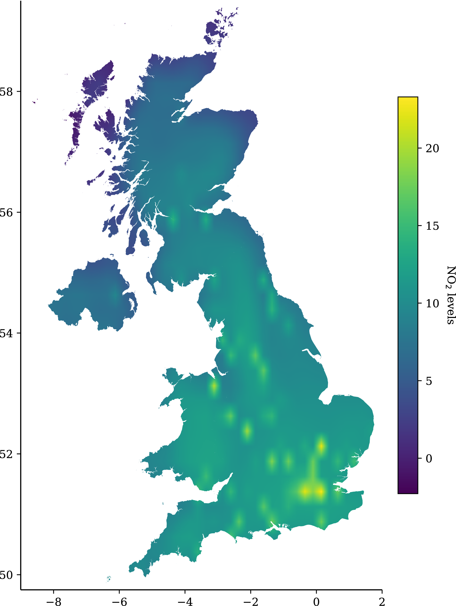
Figure 1: Inferred NO₂ spatial surface ($\mu$gm^-3) in the UK at 9AM on March 23${}^{\text{rd}}$; the day that initial lockdown measures were announced.

Reanalysis data

ERA5 is a reanalysis product developed by the European Centre for Medium Range Weather Forecasting (ECMWF). Using data assimilation techniques with a forecast model, satellite data and ground-based observations, global hourly meteorological conditions are produced at a horizontal resolution of $\approx$31 km (Hersbach et al.,, 2020), from 1979 through to the present day. Here wind speed, wind direction, relative humidity and temperature data are used to provide our model with meteorological covariate information (Grange et al.,, 2018).

In the model described in Section 3.1 we will refer to the land cover and reanalysis data as covariates, the location of the ground measurement stations as the spatial dimensions and the timestamp as the temporal dimension. This selection of covariates is consistent with other air pollution studies (e.g., Grange et al.,, 2018).

2.2 Stein variational Gaussian processes

Considering a set of $n$ observations $\mathcal{D}=\{X,\mathbf{y}\}=\{\mathbf{x}_{i},y_{i}\}_{i=1}^{n}$ where $\mathbf{x}_{i}\in\mathbb{R}^{n}$ and $y_{i}\in\mathbb{R}$. We seek to learn a function $f:\mathbb{R}^{d}\rightarrow\mathbb{R}$ that relates inputs to outputs given $\mathcal{D}$ and a likelihood function $p(\mathbf{y}\,|\,f)=\mathcal{N}(\mathbf{f},\sigma_{n}^{2})$ where $\mathbf{f}=f(X)$ is the realisation of $f$ at the input locations $X$. We place a GP prior on $f$ such that $p(f)\sim\mathcal{GP}(\mu,k_{\boldsymbol{\theta}})$, characterised by a mean function $\mu:\mathcal{X}\rightarrow\mathbb{R}$ and a $\boldsymbol{\theta}$-parameterised kernel function $k_{\boldsymbol{\theta}}:\mathcal{X}\times\mathcal{X}\rightarrow\mathbb{R}$.

To introduce sparsity into our GP model we introduce a set of inducing points $Z$ that are used to approximate $X$. This is common practice for GP modelling with large datasets as it enables tractable computation (see Snelson and Ghahramani,, 2005; Hensman et al.,, 2013). Using recent work by Pinder et al., (2020), the kernel parameters $\boldsymbol{\theta}$, observational noise $\sigma^{2}$ and latent values $\mathbf{u}=f(Z)$ of the GP can be learned using Stein Variational Gradient Descent (SVGD). Such an approach allows for highly efficient computations to be done, whilst allowing the practitioner to place prior distributions on parameters, a quality not enjoyed by regular sparse frameworks. Further, using the software package described by Pinder et al., (2020), we demonstrate how practitioners can easily integrate these models into their existing analyses. See Appendix E for an example of this.

3 Analysis

3.1 Model design

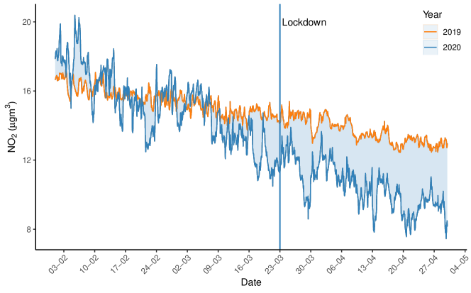
Figure 2: The difference in the inferred latent trend in 2019 and 2020 in London, United Kingdom. The start of the UK lockdown on March 23^rd is depicted by a blue vertical line.

We formulate the following kernel to capture the complex spatiotemporal dynamics of NO₂,

$$k_{\boldsymbol{\theta}}(\mathbf{x},\mathbf{x}^{\prime})=k_{1}(\mathbf{x}_{s},\mathbf{x}_{s}^{\prime})k_{2}(\mathbf{x}_{t},\mathbf{x}_{t}^{\prime})k_{3}(\mathbf{x}_{c},\mathbf{x}_{c}^{\prime})$$ (1)

where the subscripts $s$, $t$ and $c$ denote the spatial, temporal and covariate dimensions of the data. A third-order Matérn kernel is used for the spatial kernel and a squared exponential kernel for the covariate values. Furthermore, we use a product kernel of a non-stationary third-order polynomial kernel and first-order Matérn kernel for the temporal dimension. A white noise process is applied to all seven input dimensions. Full kernel expressions can be found in Appendix B.1.

The choice of kernels was driven by two factors: firstly our beliefs about the spatiotemporal behaviour of NO₂, and secondly from a comparison of the performance of several different kernels on a held-out set of data (see Appendix B.2).

To supplement the above kernel, we also equip the GP with a linear mean function $y_{i}=\mathbf{a}^{\top}\mathbf{x}_{i}+b$ where $\mathbf{a}\in\mathbb{R}^{d}$ and $b\in\mathbb{R}$. The rationale for including a linear mean function is that if we focus on the temporal dimension, there is a globally decreasing trend in NO₂ levels. Including a linear mean function provides an effective method to capture this.

3.2 Inference

From the above model design, our full set of parameters becomes $\Omega=\{\boldsymbol{\theta},\mathbf{a},b,\sigma^{2},\mathbf{u}\}$ where $|\Omega|=1022$ The learned values of these parameters are crucial as it will govern the behaviour of the inferred latent function. Within $\boldsymbol{\theta}$ we have three types of parameter: a lengthscale $\ell$ that will control the amount of correlation between datapoints, a variance $\alpha$ that controls the magnitude of the latent function and polynomial coefficients $\gamma$ that control the temporal behaviour of the GP.To learn posterior distributions for each of these parameters, we independently initialise $J=10$ particles to be used within the SVGD optimisation update step. We employ the Adam (Kingma and Ba,, 2015) optimiser to estimate step-sizes $\epsilon$ and compute the gradients using mini-batches containing 250 observations.

We fit the model from Section 3.1 to 89 days worth of hourly data from February 1${}^{\text{st}}$ to April 30${}^{\text{th}}$, noting that lockdown measures were first imposed in the UK on March 23${}^{\text{rd}}$. It is of note that enhanced social distancing was introduced in the UK from March 16${}^{\text{th}}$. A snapshot of the inferred spatial surface on March 23${}^{\text{rd}}$ at 9AM can be seen in Figure 1.

A set of 1000 inducing points $Z$ are initialised using a k-determinantal point process (KDPP) (Burt et al.,, 2020) where $k=1000$ with 10000 samples drawn according to the Markov chain Monte-Carlo (MCMC) sampler described in Anari et al., (2016). As is standard, we treat the latent values $\mathbf{u}=f(Z)$ as a model parameter.

4 Conclusions

NO₂ reduction

From the inferred latent process, we are able go beyond assessing changes in NO₂ levels at the location of measurement stations. Using the latent process we can instead compute integrated spatiotemporal mean levels. This is desirable as it gives quantities that are representative of the entire UK, and not just the parts of the UK where measurement stations exist. For the entire UK, the integrated spatial NO₂ levels decreased 36.8% between 9AM on March 16${}^{\text{th}}$ and 9AM on March 30${}^{\text{th}}$ (one week pre and post-lockdown).

Deviation from normal trends

While a clear reduction in NO₂ is apparent across the pre and post lockdown period, we would also like to give more context to the apparent decrease by comparing to levels in previous years. To define a normal trend, we consider data from February 1${}^{\text{st}}$ to April 30${}^{\text{th}}$ in 2019. Comparing the latent function that is learned in 2019 to the latent function that corresponds to data from the same period in 2020, we can see the effect that lockdown had on NO₂ levels, relative to expected temporal changes from 2019.

Quantitatively, by computing the integrated spatiotemporal mean for data from February 1${}^{\text{st}}$ through to the March 23${}^{\text{rd}}$ in 2019 and 2020, we can see that NO₂ levels are 9% lower in 2020 compared to levels in 2019. However, if we now compute the integrated spatiotemporal mean for data from March 23${}^{\text{rd}}$ through to April 30${}^{\text{th}}$ in 2019 and 2020, then we can see that levels in 2020 are now 38% lower. This can be seen in Figure 3 where we plot the difference in NO₂ levels from 2019 to 2020, integrated over the temporal values from March 23${}^{\text{rd}}$ to April 30${}^{\text{th}}$. In all locations NO₂ values are lower in 2020 when compared to 2019. Moreover, we can see that the decrease is greater in cities and the more urban areas of the UK compared to the more rural regions. For illustrative purposes, we can also see this temporal change in Figure 2. Here we observe the inferred time series at a single location (51.5^oN, 0.1^oW) that corresponds to Westminster in London, UK, where it is apparent that the divergence in NO₂ levels begins around March 23${}^{\text{rd}}$.

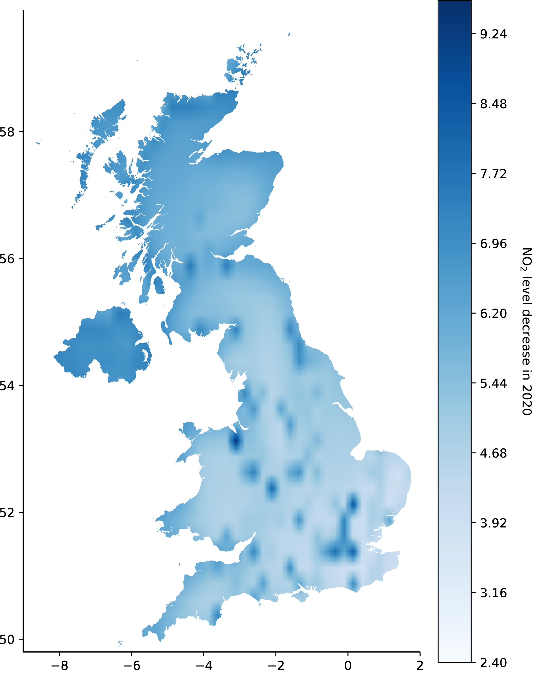
Figure 3: Difference in spatial means ($\mu$gm^-3) integrated over March 23${}^{\text{rd}}$ to April 20${}^{\text{th}}$ in 2019 and 2020. Darker shades of blue indicate a larger decrease from 2019 to 2020.

Future directions

This work has demonstrated a method to infer spatially and temporally complete air quality measurement data, which will serve machine learners, environmental scientists and policymakers. Computing spatiotemporal interpolations in the way described in this article allows us to make informed decisions based upon air quality levels in locations where we have no sensors. Further, using the associated predictive uncertainty, we can express to policy makers the confidence we have in these interpolations. Overall, this is a very powerful technique for atmospheric and environmental scientists.

Whilst we have focussed our analysis on the COVID-19 lockdown in the UK, there is nothing preventing this analysis being applied to different time periods, locations and environmental variables. For instance, this could be used in conjunction with UK-wide health data to identify regions of the UK most at risk of air quality related illnesses. Additionally, due to the accompanying uncertainty estimates in the predictive output of a GP, there is scope for this work to be used in a decision making framework to decide where new sensors should be placed. Perhaps the simplest metric for informing this decision is choosing the point location that results in the largest decrease in predictive uncertainty. Finally, this work could also provide a dataset suitable for understanding and quantifying the spatiotemporal evolution of pollution - or indeed any sparsely measured environmental variable - and for evaluating process models of the atmosphere and climate.

Appendix A Monitoring stations

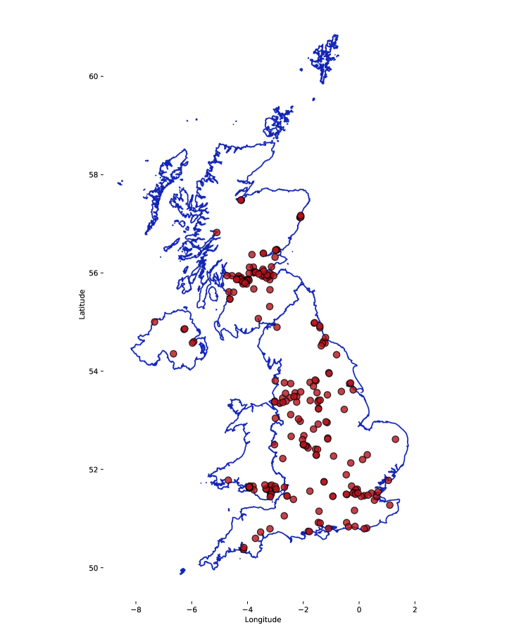
Figure 4: Spatial dispersion of the AURN, SAQN and WAQN NO₂ measurement stations described in Section 2.1.

Appendix B Kernel design

B.1 Kernels

Table 1: Explicit forms of the kernels used in Section 3 operating on an arbitrary $\mathbf{x}\in\mathbb{R}^{d}$. For Matérn kernels, the respective order is given by $\nicefrac{{c}}{{2}}-2$. For notational brevity we let $\tau=\left\lVert\mathbf{x},\mathbf{x}^{\prime}\right\rVert_{2}^{2}$.

Kernel	$k_{\boldsymbol{\theta}}(\mathbf{x},\mathbf{x}^{\prime})$	$\boldsymbol{\theta}$
Matérn $\nicefrac{{1}}{{2}}$	$\sigma^{2}\exp(\nicefrac{{-\tau}}{{\boldsymbol{\ell}}})$	$\{\sigma\in\mathbb{R},\boldsymbol{\ell}\in\mathbb{R}^{d}\}$
Matérn $\nicefrac{{5}}{{2}}$	$\sigma^{2}(1+\nicefrac{{\sqrt{5}\tau}}{{\boldsymbol{\ell}}}+\nicefrac{{\nicefrac{{5}}{{3}}\tau^{2}}}{{\boldsymbol{\ell}^{2}}})\exp(-\nicefrac{{\sqrt{5}\tau}}{{\boldsymbol{\ell}}})$	$\{\sigma\in\mathbb{R},\boldsymbol{\ell}\in\mathbb{R}^{d}\}$
Squared exponential	$\sigma^{2}\exp(\nicefrac{{-\tau}}{{2\boldsymbol{\ell}^{2}}})$	$\{\sigma\in\mathbb{R},\boldsymbol{\ell}\in\mathbb{R}^{d}\}$
Polynomial ($d$-order)	$(\sigma^{2}\mathbf{x}^{\top}\mathbf{x}^{\prime}+\gamma)^{d}$	$\{\sigma\in\mathbb{R},\gamma\in\mathbb{R}\}$
White	$\begin{cases}\sigma&\text{if $\mathbf{x}=\mathbf{x}^{\prime}$}\\ 0&\text{otherwise}\end{cases}$	$\{\sigma\in\mathbb{R}\}$

B.2 Alternative kernels

In the course of building the GP model described in Section 3, several alternative models were considered. Primarily, this is driven by the use of increasingly complex kernels whilst trying to build the most parsimonious model. Where complexity is determined by the number of parameters, we will proceed to detail the alternative kernels that were considered and their respective metrics in order of increasing complexity. 1) isotropic third-order Matérn, 2) Automatic Relevance Determination (ARD) third-order Matérn, 3) third-order polynomial kernel acting on the data’s temporal dimension convolved with an ARD third-order Matérn acting on all but the temporal dimension. In each case a zero and linear mean function are considered.

As the kernel’s complexity increased, the the marginal log-likelihood increased and the root mean-squared error on a held-out set of data decreased. Based upon these two metrics, the kernel described in Section 3 was used.

Appendix C Stein variational Gaussian processes

Building upon the GP setup in Section 2.2, we give a brief description of Stein variational Gaussian processes for the interested reader.

Following Pinder et al., (2020), we introduce a set of $J$ particles $\{\boldsymbol{\lambda}^{i}\}_{i=1}^{J}$ where $\boldsymbol{\lambda}_{i}=\{\boldsymbol{\theta},\sigma_{n}^{2},\mathbf{u}\}$. The particles are then jointly optimised according to the mapping $\mathcal{T}(\boldsymbol{\lambda}_{t})=\boldsymbol{\lambda}_{t}+\epsilon_{t}\zeta(\boldsymbol{\lambda}_{t})$ where $\mathcal{T}$ is the velocity field that yields the fastest reduction of the Kullback-Leibler divergence from the approximate posterior to the true posterior. Further, $\epsilon$ is a step-size parameter. Empirically, this velocity field can be computed by

$$\hat{\zeta}(\boldsymbol{\lambda})=\frac{1}{J}\sum^{J}_{j=1}\bigg{[}\underbrace{\kappa(\boldsymbol{\lambda}^{j}_{t},\boldsymbol{\lambda})\nabla_{\boldsymbol{\lambda}}\log p(\boldsymbol{\lambda}_{t}^{j})}_{\text{Attraction}}+\underbrace{\nabla_{\boldsymbol{\lambda}}\kappa(\boldsymbol{\lambda}_{t}^{j},\boldsymbol{\lambda})}_{\text{Repulsion}}\bigg{]}.$$ (2)

where $\kappa:\mathcal{X}\times\mathcal{X}\rightarrow\mathbb{R}$ is a kernel function, such as the radial basis function (RBF) $\kappa(\mathbf{x},\mathbf{x^{\prime}})=\sigma^{2}\exp(\nicefrac{{-\left\lVert\mathbf{x}-\mathbf{x}^{\prime}\right\rVert_{2}^{2}}}{{2\ell^{2}}})$. The first term in (2) attracts particles to areas of high probability mass in Gaussian process posterior, whereas the second term in (2) encourages diversity amongst particles. For more details, see Liu and Wang, (2016); Pinder et al., (2020).

Appendix D Training details

Prior distributions

For the lengthscale parameters present in stationary kernels we use a Gamma prior with shape and scale parameters of 1. All variance parameters are assigned a Gamma prior with shape and scale parameters of 2. For the mean function’s coefficients $\mathbf{a}$ and intercept we assign a unit Gaussian prior.

SVGD kernels

In our implementation of Kernel Stein Discrepancy (KSD) the RBF kernel is used to compute (2). The kernel’s lengthscale is estimated at each iteration of the optimisation procedure using the median rule, as per Liu and Wang, (2016).

Inducing points

The inducing points used in Section 3 are set using a KDPP as per Burt et al., (2020).

Particle initialisation

Particle initialisation is carried out by making a random draw from the respective parameter’s prior distributions.

Parameter constraints

For all parameters where positivity is a constraint (i.e. variance), the softplus transformation is applied with a clipping of $10^{-6}$, as is the default in GPFlow. Inference is then conducted on the unconstrained parameter, however, we report the re-transformed parameter i.e. the constrained representation.

Optimisation

We use the Adam optimiser (Kingma and Ba,, 2015) to optimise the set of SVGD particles. The step-size parameter is started at 0.01 for the first 500 iterations, before being reduced to 0.005 and 0.001 for a further 500 iterations per step-size.

Data preprocessing

All the data used described in Section 2.1 is standardised to zero-mean and unit standard deviation.

Data availability

The LCM 2019 land cover data is available for download from the UKCEH Environmental Information Data Centre (EIDC). The dataset for GB is available at https://doi.org/10.5285/f15289da-6424-4a5e-bd92-48c4d9c830cc and the Northern Ireland dataset is available at
https://doi.org/10.5285/2f711e25-8043-4a12-ab66-a52d4e649532. The ERA5 ECMWF data is available for download from the Copernicus Climate Change Service (CS3) Climate Data Store (CDS) at https://cds.climate.copernicus.eu/#!/search?text=ERA5&type=dataset. Near real-time air quality data from the AURN, WAQN and SAQN networks are available through the Openair R package (Carslaw and Ropkins,, 2012).

Software

All code is written in Tensorflow Abadi et al., (2016) and extends the popular Gaussian process library GPFlow (Matthews et al.,, 2017). A full implementation of the SteinGP used in Section 3 can be found at
https://github.com/thomaspinder/SteinGP and corresponding experimental notebook will be publically released on submission.

Appendix E Demo Implementation

from steingp import SteinGPR, RBF, Median, SVGD import tensorflow_probability.distributions as tfd import numpy as np import gpflow

# Define some synthetic timestamps X = np.random.uniform(-5, 5, 100).reshape(-1,1) # Simulate a response plus some noise at each timestamp y = np.sin(x) + np.random.normal(loc=0, scale=0.1, size=X.shape)

# Define model kernel = gpflow.kernels.SquaredExponential() model = SteinGPR((X, y), kernel)

# Place priors on hyperparameters model.kernel.lengthscale.prior = tfd.Gamma(1.0, 1.0) model.kernel.variance.prior = tfd.Gamma(2.0, 1.0) model.likelihood.variance.prior = tfd.Gamma(2.0, 2.0)

# Fit opt = SVGD(RBF(bandwidth=Median()), n_particles=5) opt.run(iterations = 1000)

# Predict Xtest = np.linspace(-5, 5, 500).reshape(-1, 1) theta = opt.get_particles() posterior_samples = model.predict(Xtest, theta, n_samples=5)

References

- Abadi et al., (2016) Abadi, M., Agarwal, A., Barham, P., Brevdo, E., Chen, Z., Citro, C., Corrado, G. S., Davis, A., Dean, J., Devin, M., Ghemawat, S., Goodfellow, I., Harp, A., Irving, G., Isard, M., Jia, Y., Jozefowicz, R., Kaiser, L., Kudlur, M., Levenberg, J., Mane, D., Monga, R., Moore, S., Murray, D., Olah, C., Schuster, M., Shlens, J., Steiner, B., Sutskever, I., Talwar, K., Tucker, P., Vanhoucke, V., Vasudevan, V., Viegas, F., Vinyals, O., Warden, P., Wattenberg, M., Wicke, M., Yu, Y., and Zheng, X. (2016). TensorFlow: Large-Scale Machine Learning on Heterogeneous Distributed Systems. arXiv:1603.04467 [cs]. arXiv: 1603.04467.
- Anari et al., (2016) Anari, N., Gharan, S. O., and Rezaei, A. (2016). Monte carlo markov chain algorithms for sampling strongly rayleigh distributions and determinantal point processes. In Feldman, V., Rakhlin, A., and Shamir, O., editors, Proceedings of the 29th Conference on Learning Theory, COLT 2016, New York, USA, June 23-26, 2016, volume 49 of JMLR Workshop and Conference Proceedings, pages 103–115. JMLR.org.
- Anenberg et al., (2018) Anenberg, S. C., Henze, D. K., Tinney, V., Kinney, P. L., Raich, W., Fann, N., Malley, C. S., Roman, H., Lamsal, L., Duncan, B., Martin, R. V., van Donkelaar, A., Brauer, M., Doherty, R., Jonson, J. E., Davila, Y., Sudo, K., and Kuylenstierna, J. C. (2018). Estimates of the Global Burden of Ambient PM2.5, Ozone, and NO2 on Asthma Incidence and Emergency Room Visits. Environmental Health Perspectives, 126(10):107004.
- Berman and Ebisu, (2020) Berman, J. D. and Ebisu, K. (2020). Changes in U.S. air pollution during the COVID-19 pandemic. Science of The Total Environment, 739:139864.
- Burt et al., (2020) Burt, D. R., Rasmussen, C. E., and van der Wilk, M. (2020). Convergence of Sparse Variational Inference in Gaussian Processes Regression. arXiv:2008.00323 [cs, stat]. arXiv: 2008.00323.
- Carslaw, (2020) Carslaw, D. (2020). COVID-19 and changes in air pollution. Technical report.
- Carslaw and Ropkins, (2012) Carslaw, D. C. and Ropkins, K. (2012). openair — An R package for air quality data analysis. Environmental Modelling & Software, 27-28:52–61.
- Diggle and Ribeiro, (2007) Diggle, P. and Ribeiro, P. J. (2007). Model-based Geostatistics. Springer Series in Statistics. Springer-Verlag, New York.
- Forster et al., (2020) Forster, P. M., Forster, H. I., Evans, M. J., Gidden, M. J., Jones, C. D., Keller, C. A., Lamboll, R. D., Quéré, C. L., Rogelj, J., Rosen, D., Schleussner, C.-F., Richardson, T. B., Smith, C. J., and Turnock, S. T. (2020). Current and future global climate impacts resulting from COVID-19. Nature Climate Change, pages 1–7. Publisher: Nature Publishing Group.
- Grange et al., (2018) Grange, S. K., Carslaw, D. C., Lewis, A. C., Boleti, E., and Hueglin, C. (2018). Random forest meteorological normalisation models for Swiss PM trend analysis. Atmospheric Chemistry and Physics, 18(9):6223–6239. Publisher: Copernicus GmbH.
- Henschel and Chan, (2013) Henschel, S. and Chan, G. (2013). Health risks of air pollution in Europe – HRAPIE project. New emerging risks to health from air pollution –results from the survey of experts. Technical report, World Health Organisation.
- Hensman et al., (2013) Hensman, J., Fusi, N., and Lawrence, N. D. (2013). Gaussian processes for big data. In Nicholson, A. and Smyth, P., editors, Proceedings of the Twenty-Ninth Conference on Uncertainty in Artificial Intelligence, UAI 2013, Bellevue, WA, USA, August 11-15, 2013. AUAI Press.
- Hersbach et al., (2020) Hersbach, H., Bell, B., Berrisford, P., Hirahara, S., Horányi, A., Muñoz-Sabater, J., Nicolas, J., Peubey, C., Radu, R., Schepers, D., Simmons, A., Soci, C., Abdalla, S., Abellan, X., Balsamo, G., Bechtold, P., Biavati, G., Bidlot, J., Bonavita, M., De Chiara, G., Dahlgren, P., Dee, D., Diamantakis, M., Dragani, R., Flemming, J., Forbes, R., Fuentes, M., Geer, A., Haimberger, L., Healy, S., Hogan, R. J., Hólm, E., Janisková, M., Keeley, S., Laloyaux, P., Lopez, P., Lupu, C., Radnoti, G., de Rosnay, P., Rozum, I., Vamborg, F., Villaume, S., and Thépaut, J.-N. (2020). The ERA5 global reanalysis. Quarterly Journal of the Royal Meteorological Society, 146(730):1999–2049. tex.eprint: https://rmets.onlinelibrary.wiley.com/doi/pdf/10.1002/qj.3803.
- Kingma and Ba, (2015) Kingma, D. P. and Ba, J. (2015). Adam: A method for stochastic optimization. In Bengio, Y. and LeCun, Y., editors, 3rd International Conference on Learning Representations, ICLR 2015, San Diego, CA, USA, May 7-9, 2015, Conference Track Proceedings.
- Liu and Wang, (2016) Liu, Q. and Wang, D. (2016). Stein variational gradient descent: A general purpose bayesian inference algorithm. In Lee, D. D., Sugiyama, M., von Luxburg, U., Guyon, I., and Garnett, R., editors, Advances in Neural Information Processing Systems 29: Annual Conference on Neural Information Processing Systems 2016, December 5-10, 2016, Barcelona, Spain, pages 2370–2378.
- Matthews et al., (2017) Matthews, A. G. d. G., Wilk, M. v. d., Nickson, T., Fujii, K., Boukouvalas, A., Le{\’o}n-Villagr{\’a}, P., Ghahramani, Z., and Hensman, J. (2017). GPflow: A Gaussian Process Library using TensorFlow. Journal of Machine Learning Research, 18(40):1–6.
- (17) Morton, R. D., Marston, C. G., O’Neil, A. W., and Rowland, C. S. (2020a). Land cover map 2019 (25m rasterised land parcels, n. Ireland). Publisher: NERC Environmental Information Data Centre.
- (18) Morton, R. D., Marston, C. G., O’Neil, A. W., and Rowland, C. S. (2020b). Land Cover Map 2019 (25m rasterised land parcels, GB). Publisher: NERC Environmental Information Data Centre.
- Pinder et al., (2020) Pinder, T., Nemeth, C., and Leslie, D. (2020). Stein Variational Gaussian Processes. arXiv:2009.12141 [cs, stat]. arXiv: 2009.12141.
- Schindler, (2020) Schindler, T. (2020). SVS: Reductions in Pollution Associated with Decreased Fossil Fuel Use Resulting from COVID-19 Mitigation. Technical report.
- Snelson and Ghahramani, (2005) Snelson, E. and Ghahramani, Z. (2005). Sparse gaussian processes using pseudo-inputs. In Advances in Neural Information Processing Systems 18 [Neural Information Processing Systems, NIPS 2005, December 5-8, 2005, Vancouver, British Columbia, Canada], pages 1257–1264.
- Sundvor et al., (2013) Sundvor, I., Nuria, C. B., Viana, M., Querol, X., Reche, C., Amato, F., Mellios, G., and Guerreiro, C. (2013). Road traffic’s contribution to air quality in European cities ETC/ACM Technical Paper 2012/14. Technical report.