Tracking Cells and their Lineages via Labeled Random Finite Sets

Abstract

Determining the trajectories of cells and their lineages or ancestries in live-cell experiments are fundamental to the understanding of how cells behave and divide. This paper proposes novel online algorithms for jointly tracking and resolving lineages of an unknown and time-varying number of cells from time-lapse video data. Our approach involves modeling the cell ensemble as a labeled random finite set with labels representing cell identities and lineages. A spawning model is developed to take into account cell lineages and changes in cell appearance prior to division. We then derive analytic filters to propagate multi-object distributions that contain information on the current cell ensemble including their lineages. We also develop numerical implementations of the resulting multi-object filters. Experiments using simulation, synthetic cell migration video, and real time-lapse sequence, are presented to demonstrate the capability of the solutions.

I Introduction

Tracking cells from time-lapse video data is one of the foremost tasks in developmental cell biology [1] and is critical to the understanding of the laws governing cell behavior in living tissue–laws that predict when a cell will divide or differentiate into a specialized cell type [2]. Cell tracking is a challenging problem due to intricate cell motion/interaction, cell division/death, complex sources of uncertainty, such as false positives, false negatives [3, 4, 5]. A typical time-lapse video consists of thousands of frames. Thus manually tracking the cells is time consuming and prone to human errors. Moreover, given the large and growing volume of data, it becomes necessary to automate cell tracking [6, 7, 8, 1, 4, 5, 9, 10, 11].

In addition to determining the trajectories of the cells, it is necessary to resolve their lineages or ancestries in cell divisions as time progresses. A cell’s lineage describes the sequence of ancestors of a cell and is important for the understanding of the relationship between cell ancestry and cell fate–how a particular cell develops into a final cell type [12]. Many solutions have been proposed for resolving cell lineages, see for example [12] and references therein. However, most of these methods are invasive in the sense that they require injection of dye as markers to keep track of the cells and their ancestors. Non-invasive solutions are more economically viable and suitable for almost all types of experiments.

Regardless of whether cell tracking is performed manually or automated, it is important to note that the tracking results are not perfect. Further, since cell experiments are mostly designed to infer certain variables/parameters from the estimated tracks, errors in the inferred results inevitable. How meaningful are the observations from the experiments depend on the level of confidence in the inferred results. Hence, it is important that the tracking framework has the capability to characterize confidence on the inferred information.

So far, amongst the many approaches to multi-object tracking, Mahler’s random finite set (RFS) framework [13, 14] has a demonstrable capability for characterizing confidence/uncertainty on the inferred variables/results [15]. Classical probabilistic multi-object tracking approaches such as Multiple Hypothesis Tracking (MHT) [16] and Joint Probabilistic Data Association (JPDA) [17], have been used in many applications, including cell tracking. However, while they provide some form of confidence on the estimated tracks individually, the issue of confidence on the variables inferred from the tracks have not been considered. The RFS approach has also been applied to cell tracking in [3, 5, 18, 19, 11]. In [20] a labeled RFS multi-object tracking filter that accommodates spawning was proposed. However, such spawning model does not capture ancestry in cell division, nor changes in cell appearance before dividing, hence heuristic post-processing is needed to accommodate cell ancestry [19].

In this work, we propose a tractable spawning model and multi-object tracking filters that address cell division including lineages and changes in appearance. The labeled RFS formulation [21] enables lineage information to be encoded into the labels of individual objects. Furthermore, the labels that identify individual objects and their ancestry, can be naturally assimilated into the RFS spawning models, and subsequently inferred from the data using labeled RFS estimation techniques. The salient features of the proposed spawning model is its ability to capture changes in cell appearance prior to division and cell ancestry, thereby enabling better lineage estimation. When a track is born from spontaneous birth, its label contains information pertaining to when it is born and from which birth region [21]. Similarly, for a spawned track, its label contains information pertaining to when and from which parent it originated. Under the proposed spawning model, we derive the optimal multi-object Bayes tracking filter, and two approximate filters, using moment and cardinality matching [22], as trade-offs between accuracy and computational load. Efficient implementations are developed to operate under real world conditions where the (time-varying) clutter rate and detection probability are not known. We also demonstrate the capability of our approach to quantify confidence in the inferred results.

For the remainder of the paper, we summarize related works and the RFS framework in Section II. Section III presents the novel spawning model and corresponding multi-object tracking filters. Section IV details the implementations of the cell tracking filters, and numerical studies are presented in Section V.

II Background

II-A Related Work

There are two main approaches to cell tracking, namely model evolution and track-by-detection. In model evolution, segmentation and tracking (including the deformation of shapes) are carried out simultaneously. On the other hand, track-by-detection treats detection and tracking as two separate modules.

TABLE I: List of symbols

Notation	Description
$\mathbb{X}$	single object state space
$\mathbb{L}$	label space
$\mathbb{M}$	mode space
$\mathbb{K}$	kinematic/feature space
$\boldsymbol{X}$	labeled multi-object state
$\boldsymbol{x}=(x,\ell)$	labeled single-object state (with label $\ell$)
$m$	object mode
$\zeta$	object kinematic state
$[h(\cdot)]^{X}$	set exponential
$\langle f,g\rangle$	inner product between $f$ and $g$
$\delta_{Y}[X]$	generalized Dirac delta function
$1_{Y}(X)$	set inclusion function
$\left\langle\boldsymbol{f}\right\rangle$	label marginal of $\boldsymbol{f}$
$\mathcal{L}\left(\boldsymbol{X}\right)$	set of labels of $\boldsymbol{X}$
$\mathcal{F}(X)$	class of finite subsets of $X$
$C$	maximum cardinality of generated sets
$c$	cardinality of a generated set
$\mathbb{G}_{+}^{(c)}(\ell)$	labels of set with cardinality $c$ generated by
	object labeled $\ell$
$\mathbb{G}_{+}(\ell)$	labels of all sets generated by object labeled $\ell\!\!$
$\Phi_{+}^{(c)\!}(\cdot|\boldsymbol{x})$	joint labeled state density of $c$ daughters of $\boldsymbol{x}$
$\varphi_{+}^{(c)}\left(\cdot\mid\zeta,\ell\right)$	joint kinematics-label density of $c$ daughters
	of $(\zeta,\ell)$
$\vartheta^{(c)}(m_{+}^{(i)}|m,\ell)\!\!$	mode transition probability
$\boldsymbol{g}(Z|\boldsymbol{X})$	multi-object likelihood
$\varrho$	observed kinematic feature
$\alpha$	observed appearance feature
$\gamma$	extended association map
$\Gamma$	space of (extended) association maps
$\mathbb{D}$	space of association maps with division
$\mathbb{N}$	space of association maps without division

Algorithms in the model evolution category are usually based on minimizing some energy functions via active contours [23, 24], level sets [25, 26, 27], or mean shift [28]. While this approach is accurate in tracking the cell membranes, there are a number of disadvantages. Firstly, it is domain-specific as the modeling of the contour evolution depends on the types of cell. Secondly, it is computational intensive in high cell density scenarios [29], which limits application to large scale problems. Thirdly, since the detection and tracking modules cannot be separated, these algorithms are not flexible and their performances degrade when the sampling rate is low as the deformation cannot be adequately tracked [9].

Track-by-detection infers cell tracks from the detector output, which allows the extraction of temporal information on the cell population, and the applications of different detection methods without reformulating the tracking module. Track-by-detection algorithms can be further classified as deterministic or probabilistic. Deterministic algorithms are based on deterministically matching detections to cell tracks by optimizing some cost functions [1, 30, 31, 32], and perform relatively well in scenarios where the cells are well separated. However, performance deteriorates when the clutter rate and cell density are high [4]. In probabilistic algorithms, the cell tracks are inferred from some form of probability distribution [7, 5, 4]. This approach has been demonstrated to track closely spaced cells in environments with high clutter rate and low detection probability [4].

The quality of cell detectors influences the performance of cell trackers in the track-by-detection approach. Apart from segmentation in the model evolution approach, there are generally two approaches to detect cells: morphological thresholding and machine learning. In morphological thresholding, image filtering is applied to remove noise, followed by locally adaptive thresholding [33, 34, 35, 36], and finally, size filtering to obtain cell blobs. With the advent of neural networks, machine learning for cell detection is gaining attention [37, 38, 39]. Detectors in this category are usually neural networks trained to predict enclosed boxes, segmentation masks and location of cells from input images. While promising, high computational efforts and large volumes of training data are needed to achieve reliable predictions. In practice, the morphological approach is still widely used given its speed and relative accuracy. Moreover, in fluorescence imaging, the cells are usually observed as bright/dark spots without any features, and hence rely mainly on morphological thresholding for detection.

Due to its importance in developmental cell biology, a number of cell lineage estimation techniques have been developed [40]. The tracking-free methods rely on features associated with mitotic cells to detect mitosis in individual images [41, 42, 43]. The tracking-based methods identify mitosis by integrating mitotic models/classifiers into the cell trackers [32, 44, 45, 28, 46, 47], or by post-processing the tracking results to construct the lineage tree [48]. While tracking-free methods can perform well in high mitosis abnormality levels, tracking-based methods are more advantageous when this abnormality level is weak or the image sampling rate is low.

Established approaches such as JPDA [17], MHT [16] and RFS [13, 14] have been applied to cell tracking in [3, 4, 49, 5, 50, 19]. The RFS approach models the entire ensemble of cells as an RFS, which naturally encapsulates the uncertainty in the cell population due to mitosis, migration, death, and the presence of clutter and mis-detection. More importantly, labeled RFS provides natural means for modeling cell trajectories and their lineages [15], [20]. Numerically, the RFS approach has been demonstrated on very large-scale problems [51], and hence promising for applications with high cell density.

For most multi-object trackers, detection probability and clutter rate are important prior parameters that are usually assumed known. However, in biological applications, these parameters are unknown and vary with time. RFS-based filters have been developed to address this problem in [52, 53, 54]. In [5], the robust CPHD filter [52] that estimates clutter rate and detection probability, was bootstrapped to another standard CPHD filter [55] to track cells. However, this algorithm does not consider cell division. Moreover, the robust CPHD filter [52] is superseded by the newer solution in [53].

II-B Bayesian Multi-Object Filtering

In the (classical) Bayes filter, all information on the current state $x$, modeled as a random vector, is encapsulated in the filtering density $p$ (which is conditioned on the observation history, but omitted for clarity). Moreover, this density can be propagated to the next time via the Bayes recursion [56]

$$p_{+}\!\left(x_{+}\right) = {\scriptstyle{\displaystyle{\textstyle\int}}}f_{+}\!\left(x_{+}|x\right)p\left(x\right)dx,$$ (1)

$$p_{+}\!\left(x_{+}|z_{+}\right) \propto g_{+}\left(z_{+}|x_{+}\right)p_{+}\!\left(x_{+}\right),$$ (2)

where $p_{+}\!$ is the prediction density, $f_{+}(x_{+}|x)$ is the Markov transition density to the state $x_{+}$ from a given $x$, and $g_{+}(z_{+}|x_{+})$ is the likelihood that $x_{+}$ generates an observation $z_{+}$. For simplicity we omit the subscript for current time and use the subscript ‘+’ to denote the next time step.

Cell tracking is a multi-object estimation problem because the number of cells and their states are unknown and time-varying. Thus, instead of a single state vector we have a set of state vectors, called the multi-object state. Specifically, each element of the multi-object state $\boldsymbol{X}$ is an ordered pair $\boldsymbol{x}=(x,\ell)$, where $x$ is a state vector in some space $\mathbb{X}$, and $\ell$ is a distinct label in some discrete space $\mathbb{L}$ [21]. The label of an $\boldsymbol{x\in}\mathbb{X}\times\mathbb{L}$ is given by the label extraction function $\mathcal{L}\left(\boldsymbol{x}\right)$, and the labels of any $\boldsymbol{X\subset}\mathbb{X}\times\mathbb{L}$ is defined as $\mathcal{L}\left(\boldsymbol{X}\right)\triangleq\left\{\mathcal{L}\left(\boldsymbol{x}\right):\boldsymbol{x}\in\boldsymbol{X}\right\}$.

Hereon, we adhere to the following notations:

$$\begin{array}[]{cc}[h(\cdot)]^{X}\triangleq\prod_{x\in X}h(x);&\ \ \langle f,g\rangle\triangleq\int f(x)g(x)dx;\\ \delta_{Y}[X]\triangleq\begin{cases}1&X=Y\\ 0&X\neq Y\end{cases};&\ \ 1_{Y}(X)\triangleq\begin{cases}1&X\subseteq Y\\ 0&\textrm{otherwise}\end{cases}.\end{array}$$

For a singleton $X=\{x\}$, we abbreviate $1_{Y}(x)\triangleq 1_{Y}(\{x\})$. Since the multi-object state $\boldsymbol{X}$ must have distinct labels, we require the distinct label indicator $\Delta\left(\boldsymbol{X}\right)\triangleq\delta_{\left|\boldsymbol{X}\right|}\left[\left|\mathcal{L}\left(\boldsymbol{X}\right)\right|\right]$ be equal to 1. We also denote the class of finite subsets of a space $S$ by $\mathcal{F}(S)$, and for a function $f:\mathcal{F}(\mathbb{X}\times\mathbb{L})\rightarrow\mathbb{R}$, we define its label-marginal $\left\langle f\right\rangle:\mathcal{F}(\mathbb{L})\rightarrow\mathbb{R}$, by

$$\left\langle f\right\rangle(\{\ell_{1},...,\ell_{n}\})\triangleq{\textstyle\int}f(\{(x_{1},\ell_{1}),...,(x_{n},\ell_{n})\})dx_{1:n}.$$ (3)

In line with the Bayesian paradigm, the multi-object state is modeled as a random finite set, characterized by Mahler’s multi-object density [13, 14] (equivalent to a probability density [57]). The multi-object Bayes filter takes on the same form as the classical Bayes filter with: $x$ and $x_{+}$ replaced by the sets $\boldsymbol{X}$ and $\boldsymbol{X}_{+}$ of multi-object states; $p$, $p_{+}$ and $p_{+}(\cdot|z_{+})$ replaced by the multi-object filtering/prediction densities $\mathbf{\boldsymbol{\pi}}$, $\mathbf{\boldsymbol{\pi}_{+}\!}$ and $\boldsymbol{\pi}_{+}(\cdot|Z_{+})$; $f_{+}$ and $g_{+}$ replaced by the multi-object transition density $\boldsymbol{f}_{+}$ and multi-object (observation) likelihood $\boldsymbol{g}_{+}$; $z_{+}$ replaced by the measurement set $Z_{+}$; and the vector integral replaced by the set integral [14], i.e.

$$\boldsymbol{\pi}_{+}\!\left(\boldsymbol{X}_{+}\right) = {\textstyle\int}\boldsymbol{f}_{+}\!\left(\boldsymbol{X}_{+}|\boldsymbol{X}\right)\boldsymbol{\pi}\left(\boldsymbol{X}\right)\delta\boldsymbol{X},$$ (4)

$$\boldsymbol{\pi}_{+}\!\left(\boldsymbol{X}_{+}|Z_{+}\right) \propto \boldsymbol{g}_{+}\left(Z_{+}|\boldsymbol{\boldsymbol{X}}_{+}\right)\boldsymbol{\pi}_{+}\!\left(\boldsymbol{X}_{+}\right).$$ (5)

The multi-object (observation) likelihood captures the observation noise, false negatives, and false positives. For $Z=\{z_{1:|Z|}\}$, the multi-object likelihood is given by

$$\boldsymbol{g}(Z|\boldsymbol{X})\propto\sum_{\theta\in\Theta}1_{\Theta(\mathcal{L}(\boldsymbol{X}))}(\theta)\left[\varPsi_{Z}^{(\theta)}\right]^{\boldsymbol{X}},$$ (6)

where $\Theta$ is the set of positive 1-1 maps $\theta$ taking the object labels to indices of observations, $\Theta\left(I\right)$ is the subset of $\Theta$ with domain $I$, $\varPsi_{Z}^{(\theta)}(x,\ell)=\psi_{Z}^{(\theta(\ell))}(x,\ell)$,

$$\psi_{Z}^{(j)}(x,\ell)=\begin{cases}\frac{P_{D}(x,\ell)g(z_{j}|x,\ell)}{\kappa(z_{j})}&\textrm{if }j\in\{1,...,|Z|\}\\ 1-P_{D}(x,\ell)&\textrm{if }j=0\end{cases},$$

$\kappa(\cdot)$ is the clutter intensity, $P_{D}(x,\ell)$ is the detection probability, and $g(\cdot|x,\ell)$ is the single-object likelihood function [58].

The multi-object transition density captures the motions, births and deaths of objects. Births can occur independently or spawn from parent objects. A multi-object transition density that models spawning was proposed in [20]. However, this model does not accommodate ancestry in cell division because it assumes independence between the parent’s existence and spawned objects’ existence. Specifically, a parent can survive/die independent of whether it spawns or not. This is not the case in cell division where the parent ceases to exist at the moment it spawns. Hence, the model in [20] cannot capture mitosis because it permits parents and daughters to co-exist.

III Labeled RFS Tracker for Cell Biology

This section presents a multi-object transition density that captures cell lineages (Subsection III-A), the resulting multi-object filters (Subsection III-B), and a cell division model that incorporates cell appearance (Subsection III-C). Extension to tracking with unknown clutter rate, detection probability, and birth parameters is discussed in Subsection III-D.

III-A Spawning Model for Cell Division

Following [21], the label $\ell=(k+1,\iota)$ of a spontaneous birth, i.e. a new object with no parent, comprises the time of birth, and an index to distinguish those born at the same time. Hence, the space $\mathbb{B}_{+}$ of spontaneous birth labels at time $k+1$ is $\{k+1\}\times\mathbb{I}$, where $\mathbb{I}$ is a discrete set.

An object (with label $\ell$) can generate, at the next time, a set $\mathbb{G}_{+}^{(c)}(\ell)$ of $c$ objects with distinct labels. For: $c=0$, the object dies and $\mathbb{G}_{+}^{(0)}(\ell)=\emptyset$; $c=1$, the object continues to live and $\mathbb{G}_{+}^{(1)}(\ell)=\{\ell\}$; and $c>1$, the object spawns $c$ daughters with label set $\mathbb{G}_{+}^{(c)}(\ell)=\{(\ell,k+1,c)\}\times\{1,...,c\}$, see Fig. 1. In this convention the label $(\ell,k+1,c,\iota)\in\mathbb{G}_{+}^{(c)}(\ell)$ consists of the parent label, the time of birth, the number of siblings, and an index to distinguish it amongst the siblings. Assuming $\ell$ can spawn at most $C$ daughters at a time (for cell division $C=2$ since a cell can only divide into two), the space of possible labels generated by $\ell$ is $\mathbb{G}_{+}(\ell)\triangleq\biguplus_{c=1}^{C}\mathbb{G}_{+}^{(c)}(\ell)$. We also abbreviate $\mathbb{G}_{+}(\boldsymbol{x})=\mathbb{G}_{+}(\mathcal{L}(\boldsymbol{x}))$, and $\mathbb{G}_{+}(L)\triangleq\biguplus_{\ell\in L}\mathbb{G}_{+}(\ell)$.

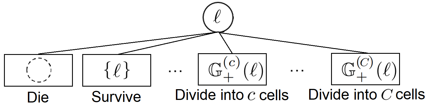
Figure 1: An object can divide into maximum of $C$ objects in the next time.

Given the current label space $\mathbb{L}$, the space of all possible labels at the next time is $\mathbb{L}_{+}=\mathbb{G}_{+}(\mathbb{L})\uplus\mathbb{B}_{+}$. Note that $\mathbb{L}=\biguplus_{\ell\in\mathbb{L}}\mathbb{G}_{+}^{(1)}(\ell)\subset\mathbb{L}_{+}$. To address lineage, we define the Parent function on $\mathbb{L}_{+}-\mathbb{B}_{+}-\mathbb{L}$ by $\text{Parent}((\ell,k+1,c,\iota))=\ell$.

Remark. There are no unique labeling conventions for spawned objects. For consistency in lineage, we require the following conditions (which our labeling convention satisfies):

1. $\mathbb{G}_{+}^{(c)}(\ell)\cap\mathbb{G}_{+}^{(c^{\prime})}(\ell^{\prime})=\emptyset$ if $\ell\neq\ell^{\prime}$, i.e. the children from two distinct objects must not share any common labels;

2. $\mathbb{G}_{+}^{(c)}(\ell)\cap\mathbb{G}_{+}^{(c^{\prime})}(\ell)=\emptyset$ if $c\neq c^{\prime}$, i.e. any two sets of children with different cardinalities, (even from the same parent), should not have common labels.

These properties enable the parent of any $\mathbb{\ell\in\mathbb{L}_{+}-\mathbb{B}_{+}-\mathbb{L}}$ to be determined as the (unique) label $\ell^{\prime}$ such that $\ell\in\mathbb{G}_{+}(\ell^{\prime})$.

The new set of objects generated from a single object with labeled state $\boldsymbol{x}$ is modeled by a labeled RFS with density:

$$\!\!\!\boldsymbol{f}_{\!G,+}(\boldsymbol{U}|\boldsymbol{x})=\Delta(\boldsymbol{U})\sum_{c=0}^{C}\delta_{\mathbb{G}_{+}^{(c)\!}(\boldsymbol{x})}[\mathcal{L}(\boldsymbol{U})]\rho_{+}^{(c)}(\boldsymbol{x})\Phi_{+}^{(c)}(\boldsymbol{U}|\boldsymbol{x}),\!\!\!\!$$ (7)

where $\rho_{+}^{(c)}(\boldsymbol{x})$ is the probability that $\boldsymbol{x}$ generates $c$ objects at the next time, and $\Phi_{+}^{(c)}(\{\boldsymbol{x}_{+}^{(1)},...,\boldsymbol{x}_{+}^{(c)}\}|\boldsymbol{x})$ is the joint density of their $c$ states, with the convention $\Phi_{+}^{(0)}(\emptyset|\boldsymbol{x})=1$. Note that parent objects cannot co-exist with their daughters, and the kinematics/features of siblings from the same parent are statistically dependent. On the other hand, in [20] parents of spawned objects can continue to exist, and the kinematics/features of siblings from the same parent are statistically independent.

It is assumed that the sets of objects generated by individual elements of a given (labeled) multi-object state $\boldsymbol{X}$ are independent of each other and the set of spontaneous births. Additionally, since all generated labels are distinct, the multi-object state $\boldsymbol{X}_{+}$ at the next time is a disjoint union of the spontaneous births and the sets of labeled states generated from different elements of $\boldsymbol{X}$. Hence, using the FISST convolution theorem [13] the multi-object transition density is given by

$$\!\!\boldsymbol{f}_{+}(\boldsymbol{X}_{+}\mid\boldsymbol{X})=\boldsymbol{f}_{B,+}(\boldsymbol{X}_{+}\cap(\mathbb{X}\times\mathbb{B}_{+}))\boldsymbol{f}_{G,+}(\boldsymbol{X}_{+}|\boldsymbol{X}),$$ (8)

where $\boldsymbol{f}_{B,+}$ is the density of the spontaneous-birth set, and

$$\!\boldsymbol{f}_{G,+}(\boldsymbol{X}_{+}|\boldsymbol{X})=\prod_{\boldsymbol{x}\in\boldsymbol{X}}\boldsymbol{f}{}_{G,+}(\boldsymbol{X}_{+}\cap(\mathbb{X}\times\mathbb{G}_{+}(\boldsymbol{x}))|\boldsymbol{x}).\!\!$$ (9)

A popular birth model is a labeled multi-Bernoulli (LMB) [21]

$$\boldsymbol{f}_{B,+}(\boldsymbol{Y}) = \Delta(\boldsymbol{Y})w_{B,+}(\mathcal{L}(\boldsymbol{Y}))[p_{B,+}]^{\boldsymbol{Y}},$$ (10)

where $w_{B,+}(L)=1_{\mathbb{B}_{+}}(L)[1-r_{B,+}]^{\mathbb{B}_{+}-L}[r_{B,+}]^{L},$ $r_{B,+}(\ell)$ is the probability of new a birth with label $\ell$, and $p_{B,+}(\cdot,\ell)$ is the probability density of its (unlabeled) state.

Remark. In addition to the above labeling scheme, our proposed dynamic model removes the independence in the parent’s existence and daughters’ existence assumed in [20]. Consequently, the techniques for propagating the multi-object filtering density used in [20] is no longer applicable.

III-B Multi-object Filtering with Cell Division

For the standard multi-object system model (no spawnings), if the initial prior is a Generalized Labeled Multi-Bernoulli (GLMB), then the prediction and filtering densities are also GLMBs, i.e. multi-object densities of the form [21]

$$\boldsymbol{\pi}\left(\boldsymbol{X}\right)=\Delta\left(\boldsymbol{X}\right)\sum_{I,\xi}\omega^{\left(I,\xi\right)}\delta_{I}[\mathcal{L}(\boldsymbol{X})]\left[p^{(\xi)}\right]^{\boldsymbol{X}},$$ (11)

where $I\in\mathcal{F}(\mathbb{L})$, $\xi\in\Xi$ the space of all association histories, each $\omega^{\left(I,\xi\right)}$ is non-negative such that $\sum_{I,\xi}\!\omega{}^{(I,\xi)}=1$, and each $p^{\left(\xi\right)}\left(\cdot,\ell\right)$ is a probability density on $\mathbb{X}$.

Hereon, we use the multi-object system model described by our proposed multi-object transition density (8) and multi-object likelihood (6). In this case the prediction and filtering densities are not GLMBs, but take on a more general form:

$$\boldsymbol{\pi}(\boldsymbol{X})=\Delta(\boldsymbol{X})\!\sum_{I,\xi}\!\omega^{(I,\xi)}\delta_{I}[\mathcal{L}(\boldsymbol{X})]p^{(\xi)}(\boldsymbol{X}),$$ (12)

where $\left\langle p^{(\xi)}\right\rangle(L)=1$, for each $L\in\mathcal{F}(\mathbb{L})$.

The RFS framework provides the tools for characterizing uncertainty in the ensemble of trajectories such as the cardinality distribution, intensity $v$, and some other statistics:

$$\Pr(\left|\boldsymbol{X}\right|\text{=}n)=\sum_{I,\xi}\delta_{n}\left[\left|I\right|\right]\omega^{(I,\xi)},$$ (13)

$$\!\!\!\!\!\!\!v(x,\ell)=\sum_{I,\xi}1_{I}(\ell)\omega^{(I,\xi)}\left\langle p^{(\xi)\!}\left(\{(x,\ell)\}\!\uplus\!(\cdot)\right)\!\right\rangle\!(I\!-\!\{\ell\}),$$ (14)

$$\!\Pr(\text{label $\ell\ $exists})=\sum_{I,\xi}1_{I}(\ell)\omega^{(I,\xi)},$$ (15)

$$\!\!\!\!\!\Pr(n\text{ new spawnings})=\sum_{I,\xi}\delta_{n\!}\left[\left|I\mathbf{\cap}(\mathbb{L}\!-\!\mathbb{L}_{-}\!-\!\mathbb{B})\right|\right]\omega^{(I,\xi)},$$ (16)

$$\!\!\!\!\!\Pr(n\text{ divisions})\!=\!\sum_{I,\xi}\delta_{n\!}\left[\left|\text{Parent}\!\left(I\mathbf{\cap}(\mathbb{L}\!-\!\mathbb{L}_{-}\!-\!\mathbb{B})\right)\right|\right]\omega^{(I,\xi)}\!.$$ (17)

From (12), trajectories are estimated by first finding a cardinality $n^{*}$ that maximizes the cardinality distribution, and the component $(I^{*},\xi^{*})$ with highest weight such that $|I^{*}|=n^{*}$. The trajectories with labels in $I^{*}$ are estimated jointly from the function $p^{(\xi^{*})}(\cdot)$. For the GLMB special case, the trajectory of each $\ell\in I^{*}$ is estimated from $p^{(\xi^{*})}(\cdot,\ell)$ [15, 59].

The propagation of the multi-object prediction and filtering densities are given in Propositions 1 and 2, respectively (see Appendix VII-A, VII-B for proof).

Proposition 1.

Given a current multi-object filtering density of the form (12), the prediction density at the next time is

$$\!\!\!\!\!\boldsymbol{\pi}_{\!+}\!(\boldsymbol{X}_{\!+})\!=\!\Delta(\boldsymbol{X}_{\!+})\!\!\sum_{I,\xi,I_{+}}\!\!\omega_{+}^{(I,\xi,I_{+\!})}\delta_{I_{+\!}}[\mathcal{L}(\boldsymbol{X}_{\!+})]p_{+}^{(I,\xi)}(\boldsymbol{X}_{\!+}),$$ (18)

where $I\subseteq\mathbb{L}$, $\xi\in\Xi$, $I_{+}\subseteq\mathbb{L}_{+}$, and

$$\!\!\!\!\!\!\!\!\!\omega_{+}^{(I,\xi,I_{+})} \!\!\!= \!\!\!\omega^{(I,\xi)}w_{B,+}(I_{+}\cap\mathbb{B}_{+})\eta_{G,+}^{(I,\xi)}(I_{+}-\mathbb{B}_{+}),$$ (19)

$$\!\!\!\!\!\!\!\!\!p_{+}^{(I,\xi)\!}(\boldsymbol{Y}) \!\!\!= \!\!\!\left[p_{B,+}\right]{}^{\boldsymbol{Y}\cap(\mathbb{X}\times\mathbb{B}_{+})}p_{G,+}^{(I,\xi)}(\boldsymbol{Y}-(\mathbb{X}\times\mathbb{B}_{+})),$$ (20)

$$\!\!\!\!\!\!\!\!\!\eta_{G,+}^{(I,\xi)}(L) \!\!\!= \!\!\!\left\langle q_{G,+}^{(I,\xi)}\right\rangle(L),$$ (21)

$$\!\!\!\!\!\!\!\!\!p_{G,+}^{(I,\xi)}(\boldsymbol{Y}) \!\!\!= \!\!\!q_{G,+}^{(I,\xi)}(\boldsymbol{Y})/\eta_{G,+}^{(I,\xi)}(\mathcal{L}(\boldsymbol{Y})),$$ (22)

$$\!\!\!\!\!\!\!\!\!q_{G,+}^{(I,\xi)}(\boldsymbol{Y}) \!\!\!= \!\!\!\left\langle p^{(\xi)}(\cdot)\boldsymbol{f}_{G,+}(\boldsymbol{Y}|\cdot)\right\rangle(I).$$ (23)

Moreover, if the current multi-object filtering density is a GLMB of the form (11), then

$$\!\!\!\!\!\!q_{G,+}^{(I,\xi)}(\boldsymbol{Y}) =\left[{\textstyle\int}p^{(\xi)\!}(x,\cdot)\boldsymbol{f}_{\!G,+\!}(\boldsymbol{Y}\!\cap\!(\mathbb{X\!}\times\!\mathbb{G}_{+}(\cdot))|x,\cdot)dx\right]^{I}\!\!\!\!.$$ (24)

Note that for component $(I,\xi,I_{+})$ of the multi-object prediction density, its weight $\omega_{+}^{(I,\xi,I_{+})}$ is the product of the previous weight, the predictive probability of the new birth label set, and the predictive probability of the label set of generated objects. Similarly, its density $p_{+}^{(I,\xi)\!}$ is the product of the predictive density of new birth objects and the predictive density of generated objects.

Proposition 2.

Given a current multi-object filtering density of the form (12), the filtering density at the next time given the multi-object measurement $Z_{+}$ is

$$\!\!\!\!\boldsymbol{\pi}_{\!+}(\boldsymbol{X}_{+}|Z_{+})\propto\\ \Delta(\boldsymbol{X}_{\!+})\!\!\sum_{I,\xi,I_{+},\theta_{+}}\!\omega_{Z_{+}}^{(I,\xi,I_{+},\theta_{+})\!}\delta_{I_{+\!}}[\mathcal{L}(\boldsymbol{X}_{\!+})]p_{Z_{+}}^{(I,\xi,\theta_{+})\!}(\boldsymbol{X}_{\!+}),$$ (25)

where $I\subseteq\mathbb{L}$, $\xi\in\Xi$, $I_{+}\subseteq\mathbb{L}_{+},\theta_{+}\in\Theta_{+}$,

$$\!\!\!\!\!\!\!\!\!\omega{}_{Z_{+}}^{(I,\xi,I_{+},\theta_{+})} \!\!\!\!\!= \!\!\!\!\!\omega_{+}^{(I,\xi,I_{+})}1_{\Theta_{+}(I_{+})}(\theta_{+})\times$$ (26)

$$\!\!\!\!\!\left[\eta_{B,Z_{+}}^{(\theta_{+})}\right]^{I_{+}\cap\mathbb{B}_{+}}\eta_{G,Z_{+}}^{(I,\xi,\theta_{+})}(I_{+}-\mathbb{B}_{+}),$$

$$\!\!\!\!\!\!\!\!\!\eta_{B,Z_{+}}^{(\theta_{+})}(\ell) \!\!\!\!\!= \!\!\!\!\!\left\langle p_{B,+}(\cdot,\ell),\varPsi_{Z_{+}}^{(\theta_{+})}(\cdot,\ell)\right\rangle,$$ (27)

$$\!\!\!\!\!\!\!\!\!\eta_{G,Z_{+}}^{(I,\xi,\theta_{+})}(L) \!\!\!\!\!= \!\!\!\!\!\left\langle p_{G,+}^{(I,\xi)}(\cdot)\left[\varPsi_{Z_{+}}^{(\theta_{+})}\right]{}^{(\cdot)}\right\rangle(L),$$ (28)

$$\!\!\!\!\!\!\!\!\!p_{Z_{+}}^{(I,\xi,\theta_{+})\!}(\boldsymbol{Y}) \!\!\!\!\!= \!\!\!\!\!\left[p_{B,Z_{+}}^{(\theta_{+})}\!\right]\!^{\!\boldsymbol{Y}\cap(\mathbb{X}\!\times\!\mathbb{B}_{+\!})}p_{G,Z_{+}}^{(I,\xi,\theta_{+})\!}(\boldsymbol{Y}\!-\!(\mathbb{X}\!\times\!\mathbb{B}_{+\!})),\!\!$$ (29)

$$\!\!\!\!\!\!\!\!\!p_{B,Z_{+}}^{(\theta_{+})}(x,\ell) \!\!\!\!\!\propto \!\!\!\!\!p_{B,+}(x,\ell)\varPsi_{Z_{+}}^{(\theta_{+})}(x,\ell),$$ (30)

$$\!\!\!\!\!\!\!\!\!p_{G,Z_{+}}^{(I,\xi,\theta_{+})}(\boldsymbol{Y}) \!\!\!\!\!\propto \!\!\!\!\!p_{G,+}^{(I,\xi)}(\boldsymbol{Y})\left[\varPsi_{Z_{+}}^{(\theta_{+})}\right]{}^{\boldsymbol{Y}}.$$ (31)

Assuming that component $(I,\xi,I_{+},\theta_{+})$ of the multi-object filtering density has valid association map $\theta_{+}$, i.e. $1_{\Theta_{+}(I_{+})}(\theta_{+})=1$, then its weight $\omega{}_{Z_{+}}^{(I,\xi,I_{+},\theta_{+})}$ is the product of the predictive weight, the data-updated weight of the new birth label set, and data-updated weight of the label set of generated objects. Similarly, its density $p_{Z_{+}}^{(I,\xi,\theta_{+})\!}$ is the product of the data-updated new birth object density and the data-updated density of generated objects.

Unlike the GLMB recursion, propagating the multi-object filtering density (25) is numerically intensive, due to the growing number of high-dimensional densities over time. To alleviate this problem, we present two GLMB approximation strategies based on prediction and update approximations.

Prediction Approximation

This strategy approximates the prediction density by a GLMB using Proposition 2 of [22], and then performs an (exact) GLMB update [21] to yield a GLMB approximate filtering density, as summarized in Corollary 3.

Corollary 3.

A GLMB that matches the prediction density (18) in first moment and cardinality distribution is given by

$$\!\!\widehat{\boldsymbol{\pi}}_{+}(\boldsymbol{X}_{+})=\enskip\enskip\enskip\enskip\qquad\qquad\qquad\enskip\qquad\qquad\qquad\qquad$$

$$\Delta(\boldsymbol{X}_{\!+})\!\!\sum_{I,\xi,I_{+}}\!\!\omega_{+}^{(I,\xi,I_{+})}\delta_{I_{+\!}}[\mathcal{L}(\boldsymbol{X}_{\!+})]\left[p_{+}^{(I,\xi,I_{+})}\right]^{\boldsymbol{X}_{\!+}}\!\!\!\!,$$ (32)

where $I\subseteq\mathbb{L}$, $\xi\in\Xi$, $I_{+}\subseteq\mathbb{L}_{+}$, and

$$\!\!\!\!\!\!\!\!\!p_{+}^{(I,\xi,I_{+})}(x,\ell) \!\!\!\!\!= \!\!\!\!\!\begin{cases}p_{B,+}(x,\ell),&\ell\in\mathbb{B}_{+}\\ p_{G,+}^{(I,\xi,I_{+}-\mathbb{B}_{+})}(x,\ell),&\ell\notin\mathbb{B}_{+}\end{cases},$$ (33)

$$\!\!\!\!\!\!\!\!\!p_{G,+}^{(I,\xi,L)}(x,\ell) \!\!\!\!\!= \!\!\!\!\!1_{L}(\ell)\!\left\langle p_{G,+}^{(I,\xi)}\!\left(\{(x,\ell)\}\uplus(\cdot)\right)\!\right\rangle\!(L-\{\ell\}).$$ (34)

Moreover, if (32) is the prediction density, then the GLMB filtering density given the multi-object measurement $Z_{+}$ is

$$\!\!\!\!\!\boldsymbol{\tilde{\pi}}_{+}(\boldsymbol{X}_{+}|Z_{+})\propto\qquad\qquad\qquad\qquad\enskip\qquad\qquad\qquad\qquad$$

$$\Delta(\boldsymbol{X}_{\!+})\!\!\!\sum_{I,\xi,I_{+},\theta_{+}}\!\!\!\tilde{\omega}_{Z+}^{(I,\xi,I_{+},\theta_{+})}\delta_{I_{+\!}}[\mathcal{L}(\boldsymbol{X}_{\!+})]\!\left[\tilde{p}_{Z_{+}}^{(I,\xi,I_{+},\theta_{+})}\right]^{\boldsymbol{X}_{+}}\!\!\!\!,$$ (35)

where $I\subseteq\mathbb{L}$, $\xi\in\Xi$, $I_{+}\subseteq\mathbb{L}_{+},\theta_{+}\in\Theta_{+}$, and

$$\!\!\!\!\!\!\tilde{\omega}{}_{Z_{+}}^{(I,\xi,I_{+},\theta_{+})} \!\!\!\!\!= \!\!\!\!\!\omega_{+}^{(I,\xi,I_{+})}1_{\Theta_{+}(I_{+})}(\theta_{+})\times$$ (36)

$$\!\!\!\!\!\left[\eta_{B,Z_{+}}^{(\theta_{+})}\right]^{I_{+}\cap\mathbb{B}_{+}}\left[\tilde{\eta}_{G,Z_{+}}^{(I,\xi,I_{+},\theta_{+})}\right]^{(I_{+}-\mathbb{B}_{+})}\!\!,$$

$$\!\!\!\!\!\!\tilde{\eta}_{G,Z_{+}}^{(I,\xi,I_{+},\theta_{+})}(\ell) \!\!\!\!\!= \!\!\!\!\!\left\langle p_{G,+}^{(I,\xi,I_{+})}(\cdot,\ell),\varPsi_{Z_{+}}^{(\theta_{+})}(\cdot,\ell)\right\rangle,$$ (37)

$$\!\!\!\!\!\!\tilde{p}_{Z_{+}}^{(I,\xi,I_{+},\theta_{+})}(x,\ell) \!\!\!\!\!\propto \!\!\!\!\!p_{+}^{(I,\xi,I_{+})}(x,\ell)\varPsi_{Z_{+}}^{(\theta_{+})}(x,\ell).$$ (38)

Update Approximation

This strategy performs a joint prediction and update, followed by a GLMB approximation with matching first moment and cardinality distribution using Proposition 2 of [22], as summarized in Corollary 4.

Corollary 4.

A GLMB that matches the filtering density (25) in first moment and cardinality distribution is given by

$$\!\!\!\!\widehat{\boldsymbol{\pi}}_{\!+}(\boldsymbol{X}_{+}|Z_{+})\propto\qquad\qquad\qquad\qquad\enskip\qquad\qquad\qquad\qquad$$

$$\Delta(\boldsymbol{X}_{\!+})\!\!\!\!\!\sum_{I,\xi,I_{+},\theta_{+}}\!\!\!\!\omega_{Z_{+}}^{(I,\xi,I_{+},\theta_{+})}\delta_{I_{+\!}}[\mathcal{L}(\boldsymbol{X}_{\!+})]\left[p_{Z_{+}}^{(I,\xi,I_{+},\theta_{+})}\right]^{\boldsymbol{X}_{\!+}}\!\!\!\!,$$ (39)

where $I\subseteq\mathbb{L}$, $\xi\in\Xi$, $I_{+}\subseteq\mathbb{L}_{+},\theta_{+}\in\Theta_{+}$, and

$$\!\!\!\!\!\!\!\!\!\!p_{Z_{+}}^{(I,\xi,I_{+},\theta_{+\!})\!}(x,\ell) \!\!\!\!\!= \!\!\!\!\!\begin{cases}p_{B,Z_{+}}^{(\theta_{+})}(x,\ell),&\ell\in\mathbb{B}_{+}\\ p_{G,Z_{+}}^{(I,\xi,I_{+}-\mathbb{B}_{+},\theta_{+})}(x,\ell),&\ell\notin\mathbb{B}_{+}\end{cases},$$ (40)

$$\!\!\!\!\!\!\!\!\!\!\!p_{G,Z_{+}}^{(I,\xi,L,\theta_{+}\!)\!}(x,\ell) \!\!\!\!\!= \!\!\!\!\!1_{\!L}(\ell)\!\left\langle\!p_{G,Z_{+}}^{(I,\xi,\theta_{+\!})\!}\!\left(\{(x,\ell)\}\!\uplus\!(\cdot)\right)\!\right\rangle\!(L\!-\!\{\ell\}).$$ (41)

In principle, (39) provides a more accurate approximation to the multi-object filtering density (25) than (35). However, it is more expensive to compute due to the joint densities in (28). Nonetheless, it is cheaper than propagating (25), because the GLMB approximation caps the dimension of the joint densities.

Remark. Since the number of components in the multi-object density grows exponentially over time, truncation of its components is needed to maintain tractability. Separate prediction and update implementation is structurally inefficient because it requires two independent truncations of the multi-object densities. Since the predicted multi-object density is truncated separately from the update, computations would be wasted in updating the predicted components that generate negligible updated components. Algebraically, the prediction and update can be combined into a single expression to improve efficiency because truncation of the prediction is no longer needed [60].

III-C Cell Appearance in Mitosis

A cell can be in either the normal mode or the mitotic (about to divide) mode, in which its biological structure changes drastically. This is manifested via changes the cell’s appearance such as shape and intensity, see Fig. 2. The proposed multi-object modeling/estimation framework allows us to exploit the observed cell appearance to infer the cell modes, which, in turn improves detection of mitosis events and lineage estimation.

To capture differences in cell appearance between the two modes, we augment each cell’s unlabeled state vector with a mode variable, i.e. $x=(\zeta,m)\in\mathbb{X=K}\times\mathbb{M}$, where $\mathbb{K}$ is the kinematic/feature space, and $\mathbb{M=}\{1,2\}$ is the mode space with ‘1’ and ‘2’ representing the normal and mitotic modes, respectively. The single object observation $z=(\varrho,\alpha)$ consists of the vector $\varrho$ of kinematic features (e.g. centroid, velocity), and the vector $\alpha$ of observed appearance features (e.g. intensity, shapes, or features extracted via a neural network). To model the dependence of the cell’s appearance on the mode, we propose an observation likelihood function of the form

$$g(\varrho,\alpha|\zeta,m,\ell)=g^{(k)}(\varrho|\zeta,\ell)g^{(a)}(\alpha|\zeta,m,\ell),$$ (42)

where the kinematic likelihood $g^{(k)}(\varrho|\zeta,\ell)$ is the probability density of the observed kinematic vector, and the appearance likelihood $g^{(a)}(\alpha|\zeta,m,\ell)$ is the probability density of the observed appearance vector. Note that $g^{(k)}(\varrho|\zeta,\ell)$ is independent of the mode, while $g^{(a)}(\alpha|\zeta,m,\ell)$ is parameterized by the mode $m$. The relationship between an object’s observed appearance and its state is complex in general, and the appearance likelihood is usually constructed from training data.

The time evolution of the mode-augmented state is modeled as a jump-Markov system [53]. Specifically, our model assumes that if a cell is currently in survival mode, then at the next time step it will follow the standard motion model, but could assume either mode. If it is currently in mitotic mode, then it will divide at the next time step into daughter cells (and cease to exist). Hence, the kinematic of an existing cell can only follow the standard motion model. Effectively, the kinematics of cells are independent of the mode of their generator, and that their modes are independent of the kinematics of their generator. As a result, the density $\Phi_{+}^{(c)}$ in the cell division model (7) has the form

$$\!\!\!\!\Phi_{+}^{(c)\!}(\{(\zeta_{+}^{(1)}\!,m_{+}^{(1)}\!,\ell_{+}^{(1)}),...,(\zeta_{+}^{(c)}\!,m_{+}^{(c)}\!,\ell_{+}^{(c)})\}|(\zeta,m,\ell))=\\ \!\!\!\varphi_{+}^{(c)}(\{(\zeta_{+}^{(1)}\!,\ell_{+}^{(1)}),...,(\zeta_{+}^{(c)}\!,\ell_{+}^{(c)})\}|\zeta,\ell)\prod_{i=1}^{c}\vartheta^{(c)}(m_{+}^{(i)}|m,\ell),\!\!\!$$ (43)

where $\varphi_{+}^{(c)}\left(\cdot\mid\zeta,\ell\right)$ is the joint density of kinematics and labels of the $c$ cells generated at the next time, and $\vartheta^{(c)}(m_{+}^{(i)}|m,\ell)$ is the probability that the generated cell with label $\ell_{+}^{(i)}$ takes on mode $m_{+}^{(i)}$. Note that for $c=1,$ $\vartheta^{(1)}(m_{+}^{(1)}|m,\ell)$ is the mode transition probability of the cell with label $\ell$, if it survives.

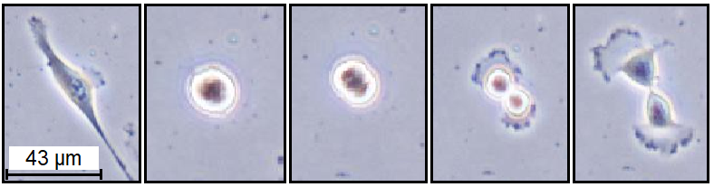
Figure 2: A breast cancer cell during mitosis.

III-D Extension to Unknown Background and Birth Parameters

To address the unknown clutter rate, we adopt the strategy proposed in [53], which treats clutter as an independent type of objects. In our context, a clutter object cannot divide and only take on one mode (normal mode) while its kinematic state is uniformly distributed over the observation region. To address the unknown cell detection rate, we augment $d\in[0,1]$ to the state of the object, i.e. $\boldsymbol{x}=(\zeta,m,d,\ell)$, and define $P_{D}(\zeta,m,d,\ell)\triangleq d$ [52]. The clutter detection rate is assumed to be a constant $P_{D}^{(0)}$ and the cell detection rate is modeled with a beta distribution which is propagated as in [52].

A static LMB birth model can be slow in initiating tracks. This can be alleviated by an adaptive LMB birth model that uses previous measurements to construct the LMB parameters at the current time step [61, 51]. Additionally, as new cells tend to enter the tracking region from the edges, the existence probability of new births can be adjusted accordingly, i.e. higher toward the edge of the image and low near the center.

IV Cell Tracking Filter Implementations

This section details the implementations of the cell tracking filters discussed in Subsection III-B. The proposed spawning model allows an object to generate up to $C$ objects, but for cell tracking we only need the special case $C=2$. Nonetheless, the solutions presented here readily extend to larger $C$.

The most pressing implementation issue is the exponential growth in the number of terms/components of the filtering densities. To maintain tractability, we truncate the insignificant (low-weight) components, which minimizes the $L_{1}$-error from the original GLMB [58]. In Subsection IV-A, we formulate the ranked assignment problem for truncating the multi-object densities in Corollary 3 (prediction approximation) and Corollary 4/Proposition 2 (update approximation/exact filtering). Since the problem size is very large, traditional ranked assignment solutions [58] are not tractable while the Gibbs sampler of [60] is not directly applicable due to the conditional parent-daughter dependence. In Subsection IV-B, we propose a block Gibbs sampling solution that can accommodate this dependence. Computing the single-object densities of the resulting GLMB is discussed in Subsection IV-C.

IV-A Ranked Assignment Problem

$$\!\!\!\!\lambda_{i}^{(I,\xi)}(j) \triangleq\begin{cases}\eta_{G,+}^{(\ell_{i},\xi)}(\emptyset),&\!\ell_{i}\in I;j\in\mathbb{N}_{+};j^{(3)}=-1,\\ \eta_{G,+}^{(\ell_{i},\xi)}(\{\ell_{i}\})\eta_{G,Z_{+}}^{(\ell_{i},\xi,\{\ell_{i}\})}(j^{(3)},\ell_{i}),&\!\ell_{i}\in I;j\in\mathbb{N}_{+};j^{(3)}>-1,\\ \eta_{G,+}^{(\ell_{i},\xi)}(\{\ell_{i}^{(1)},\ell_{i}^{(2)}\})\prod_{q=1}^{2}\eta_{G,Z_{+}}^{(\ell_{i},\xi,\{\ell_{i}^{(1)},\ell_{i}^{(2)}\})}(j^{(q)},\ell_{i}^{(q)}),&\!\ell_{i}\in I;j\in\mathbb{D}_{+};\left(\left(j^{(1)}\neq j^{(2)}\right)\textrm{or}\left(j^{(1)}=j^{(2)}=0\right)\right),\\ 1-r_{B,+}(\ell_{i}),&\!\ell_{i}\in\mathbb{B_{+}};j\in\mathbb{N}_{+};j^{(3)}=-1,\\ r_{B,+}(\ell_{i})\langle p_{+}^{(B)}(\cdot,\ell_{i})\psi_{Z_{+}}^{(j^{(3)})}(\cdot,\ell_{i})\rangle,&\!\ell_{i}\in\mathbb{B}_{+};j\in\mathbb{N}_{+};j^{(3)}>-1,\\ 0&\!\textrm{otherwise}.\end{cases}$$ (44)

Since the maximum number of daughter cells is 2 ($C=2$), we denote the set of possible labels generated at the next time from any $\ell\in\mathbb{L}$ as $\{\ell^{(1)},\ell^{(2)},\ell^{(3)}\}$, where $\ell^{(1)}=(\ell,k+1,2,1)$, $\ell^{(2)}=(\ell,k+1,2,2)$, are the daughter labels, and $\ell^{(3)}=\ell$ is the parent label (see Subsection III-A).

Note from the recursions (35) and (39) that each GLMB component (indexed by) $(I,\xi)$ generates, at the next time, a set of “children” components $(I,\xi,I_{+},\theta_{+})$. For a prior component $(I,\xi)$, let us enumerate $Z_{+}=\{z_{1:M}\}$, $I=\{\ell_{1:R}\}$, $\mathbb{B}_{+}=\{\ell_{R+1:P}\}$, and represent each pair $(I_{+},\theta_{+})\in\mathcal{F}(\mathbb{L}_{+})\times\Theta_{+}$ by $P\times 3$ matrix $\gamma$, called an extended association map, defined as

$$\gamma_{i,q}=\begin{cases}\theta_{+}(\ell_{i}^{(q)}),&\ell_{i}^{(q)}\in I_{+}\\ -1,&\textrm{otherwise }\end{cases}.$$ (45)

We use the notation $\gamma_{i}$ for the $i$-th row of $\gamma$. In this representation $\gamma_{i,q}=-1$ means $\ell_{i}^{(q)}$ does not exist, $\gamma_{i,q}=0$ means $\ell_{i}^{(q)}$ exists but not detected, and $\gamma_{i,q}>0$ means $\ell_{i}^{(q)}$ exists and generates the measurement indexed by $\gamma_{i,q}$. Since a parent cell cannot co-exist with its daughters, each $\gamma_{i}\in\mathbb{D}_{+}\uplus\mathbb{N}_{+}$, and $\gamma_{i}\in\mathbb{N}_{+}$ for $i\in\{R+1\colon P\}$, where

$$\mathbb{D}_{+}=\{0\colon M\}^{2}\times\{-1\},$$

(i.e. division occurs, daughters exist but not the parent) and

$$\mathbb{N}_{+}=\{-1\}\times\{-1\}\times\{-1\colon M\},$$

(i.e. no division). $\gamma$ also inherits the positive 1-1 property, i.e. there are no distinct $(i,q),(i^{\prime},q^{\prime})$ with $\gamma_{i,q}=\gamma_{i^{\prime},q^{\prime}}>0$.

Let $\Gamma$ denote the set of all extended association maps, i.e. $P\times 3$ matrices that are positive 1-1 with $\gamma_{i}\in\mathbb{D}_{+}\uplus\mathbb{N}_{+}$, $i\in\{1\colon R\}$ and $\gamma_{i}\in\mathbb{N}_{+}$, $i\in\{R+1\colon P\}$. Then, for any $\gamma\in\Gamma$, we recover $(I_{+},\theta_{+})$ by

$$I_{+}=\{\ell_{i}^{(q)}\in\mathbb{G}_{+}(I)\uplus\mathbb{B}_{+}:\gamma_{i,q}\geq 0\},\ \ \theta_{+}(\ell_{i}^{(q)})=\gamma_{i,q}.$$

Hence, there is a 1-1 correspondence between $\Theta_{+}(I_{+})$ and $\Gamma$, with $1_{\Gamma}(\gamma)=1_{\Theta_{+}(I_{+})}(\theta_{+})$. Consequently, selecting the significant children of component $(I,\xi)$ amounts to selecting extended association maps with significant weights as per (36) for the prediction approximation, or (26) for the update approximation.

Prediction Approximation

Since we are using a GLMB approximation, it can be shown that the weight (36) takes the form (for completeness details are given in Appendix VII-C)

$$\!\!\!\!\tilde{\omega}{}_{Z_{+}}^{(I,\xi,I_{+},\theta_{+})}\propto 1_{\Theta_{+}(I_{+})}(\theta_{+})[\eta_{G,Z_{+}}^{(\cdot,\xi,\theta_{+},I_{+})}]^{I}[1-r_{B,+}(\cdot)]{}^{\mathbb{B}_{+}-I_{+}}\\ \begin{array}[]{c}\times\left[r_{B,+}(\cdot)\!\int p_{+}^{(B)}(x,\cdot)\psi_{Z_{+}}^{(\theta_{+}(\cdot))}(x,\cdot)dx\right]^{\!I_{+}\cap\mathbb{B}_{+}},\end{array}$$ (46)

where

$$\!\!\!\!\!\!\!\!\!\!\eta_{G,Z_{+}}^{(\ell,\xi,\theta_{+},I_{+})}\!\!\!\! = \!\!\!\!\eta_{G,+}^{(\ell,\xi)}(I_{+}\cap\mathbb{G}_{+}(\ell))\times$$

$$\!\!\!\!\left[\eta_{G,Z_{+}}^{(\ell,\xi,I_{+}\cap\mathbb{G}_{+}(\ell))}(\theta_{+}(\cdot),\cdot)\right]^{I_{+}\cap\mathbb{G}_{+}(\ell)},$$

$$\!\!\!\!\!\!\!\!\!\!\eta_{G,+}^{(\ell,\xi)}(L)\!\!\!\! = \!\!\!\!\langle q_{G,+}^{(\ell,\xi)}\rangle(L),$$ (48)

$$\!\!\!\!\!\!\!\!\!\!\eta_{G,Z_{+}}^{(\ell,\xi,L)}(j,u)\!\!\!\! = \!\!\!\!\langle p_{G,+}^{(\ell,\xi,L)}(\cdot,u),\psi_{Z_{+}}^{(j)}(\cdot,u)\rangle,$$ (49)

$$\!\!\!\!\!\!\!\!\!\!p_{G,+}^{(\ell,\xi,L)}(x,u)\!\!\!\! = \!\!\!\!1_{L}(u)\!\left\langle p_{G,+}^{(\ell,\xi)}\!\left(\{(x,u)\}\uplus(\cdot)\right)\!\right\rangle\!(L-\{u\}),$$ (50)

$$\!\!\!\!\!\!\!\!\!\!p_{G,+}^{(\ell,\xi)}(\boldsymbol{Y})\!\!\!\! = \!\!\!\!q_{G,+}^{(\ell,\xi)}(\boldsymbol{Y})/\eta_{G,+}^{(\ell,\xi)}(\mathcal{L}(\boldsymbol{Y})),$$ (51)

$$\!\!\!\!\!\!\!\!\!\!q_{G,+}^{(\ell,\xi)}(\boldsymbol{Y})\!\!\!\! = \!\!\!\!\int\!p^{(\xi)\!}(x,\ell)\boldsymbol{f}_{+}^{(G)\!}(\boldsymbol{Y}\!\cap\mathbb{X\!}\times\!\mathbb{G}_{+}(\ell)|x,\ell)dx.$$ (52)

Further, using (45), we can write the weight $\tilde{\omega}_{Z_{+}}^{(I,\xi,I_{+},\theta_{+})}$ in (46) as a function of $\gamma$.

Proposition 5.

For each $i\in\{1\colon P\}$ and triplet $j\in\mathbb{D}_{+}\uplus\mathbb{N}_{+}$, define $\lambda_{i}^{(I,\xi)}(j)$ by (44). Then for any $(I_{+},\theta_{+})\in\mathcal{F}(\mathbb{L}_{+})\times\Theta_{+}$ and its equivalent representation $\gamma\in\Gamma$,

$$\tilde{\omega}_{Z_{+}}^{(I,\xi,I_{+},\theta_{+})}=\omega^{(I,\xi)}1_{\Gamma}(\gamma)\prod_{i=1}^{P}\lambda_{i}^{(I,\xi)}(\gamma_{i}).$$ (53)

Hence, for a given component $\left(I,\xi\right)$ the problem of selecting its $T$ children with highest weights according to (53) is a ranked assignment problem with cost $C_{i,j}=\lambda_{i}^{(I,\xi)}(j)$, $i\in\{1\colon P\}$, $j\in\mathbb{D}_{+}\uplus\mathbb{N}_{+}$. Note that for each $i$, there are $(M+1)^{2}+M+2$ candidate $j$’s. This ranked assignment problem can be solved using Murty’s algorithm and variants with complexity $\mathcal{O}(T(2P+M^{2}){}^{3})$ [62, 63, 64], which is still very prohibitive even for a moderate number of cells. A cheaper alternative is to sample from (53) as detailed in Subsection IV-B.

Update Approximation/Exact Filtering Density

A similar ranked assignment problem can be formulated for truncating the multi-object filtering density (25) and its GLMB approximation, by expressing the weight $\omega_{Z_{+}}^{(I,\xi,I_{+},\theta_{+})}$ (26) as a function of the extended association map. However, computing the cost $C_{i,j}$ , $i\in\{1\colon P\}$, $j\in\mathbb{D}_{+}\uplus\mathbb{N}_{+}$ for this ranked assignment problem is expensive because it involves operating on the joint densities of the cells. Hence, solving the resulting ranked assignment problem is impractical when the number of measurements $M$ is large. To circumvent this computational problem, we propose to sample the extended association maps from (53) to generate the significant children components $(I,\xi,I_{+},\theta_{+})$, and recompute their weights via (26). The rationale is that $[\tilde{\eta}_{G,Z_{+}}^{(I,\xi,I_{+},\theta_{+})}]^{(I_{+}-\mathbb{B}_{+})}$ in (36) was designed to approximate $\eta_{G,Z_{+}}^{(I,\xi,\theta_{+})}(I_{+}-\mathbb{B}_{+})$ in (26). Hence, if $(I,\xi,I_{+},\theta_{+})$ has a significant $\tilde{\omega}_{Z_{+}}^{(I,\xi,I_{+},\theta_{+})}$ it also has a significant $\omega_{Z_{+}}^{(I,\xi,I_{+},\theta_{+})}$, even though these values may differ.

IV-B Block Gibbs Sampling

This section presents a technique for sampling extended association maps from the discrete probability distribution $\pi$ given by

$$\pi(\gamma)\propto 1_{\Gamma}(\gamma)\prod_{i=1}^{P}\lambda_{i}^{(I,\xi)}(\gamma_{i}).$$ (54)

In particular, we use a block Gibbs sampler to generate $\gamma$ row by row, via a Markov chain with transition kernel

$$\pi(\gamma^{\prime}|\gamma)=\prod_{n=1}^{P}\pi_{n}(\gamma_{n}^{\prime}|\gamma_{1:n-1}^{\prime},\gamma_{n+1:P}),$$ (55)

where each conditional $\pi_{n}\left(\cdot|\cdot\right)$ is given by

$$\pi_{n}\left(\gamma_{n}^{\prime}|\gamma_{1:n-1}^{\prime},\gamma_{n+1:P}\right)=\frac{\pi\left(\gamma_{1:n}^{\prime},\gamma_{n+1:P}\right)}{\sum_{\gamma_{n}}\!\pi\left(\gamma_{1:n-1}^{\prime},\gamma_{n},\gamma_{n+1:P}\right)}.$$ (56)

The following proposition provides closed form expressions for the conditionals that can be computed/sampled at low cost. The proof follows that of Proposition 3 in [60] and is provided in Appendix VIII for completeness.

Proposition 6.

Given $n\in\{1\colon P\}$ and $\gamma_{\bar{n}}=(\gamma_{1:n-1},\gamma_{n+1:P})$,

$$\!\pi_{n}(\gamma_{n}|\gamma_{\bar{n}})\propto\begin{cases}0,&\!\!\!\!\!\begin{array}[]{l}\textrm{if any positive entry of $\gamma_{n}$ }\\ \textrm{coincides with those of }\gamma_{\bar{n}}\end{array}\\ \lambda_{n}^{(I,\xi)}(\gamma_{n}),&\!\!\textrm{otherwise}\end{cases}\!\!.\!\!$$ (57)

All iterates of the proposed block Gibbs sampler, summarized in Algorithm 1, are extended association maps. Its convergence property is given in the following proposition (the proof follows that of Proposition 4 in [60] and is provided in Appendix IX).

   Input: $\gamma^{(1)}$, $T$, $\lambda^{(I,\xi)}=\left[\lambda_{i}^{(I,\xi)}(j\in\mathbb{N}_{+}\uplus\mathbb{D}_{+})\right]$

   Output: $\gamma^{(1)},...,\gamma^{(T)}$

 

for $t=2:T$

for $i=1:P$

for $j\in\mathbb{N}_{+}\uplus\mathbb{D}_{+}$$\left(\left|\mathbb{N}_{+}\uplus\mathbb{D}_{+}\right|=(M+1)^{2}+M+2\right)$

if any positive entry of $j$ in $\left[\gamma_{1:i-1}^{(t)},\gamma_{i+1:P}^{(t-1)}\right]$

$\quad\lambda_{i}^{(I,\xi)}(j):=0$

end

end

$\quad\quad\quad\gamma_{i}^{(t)}\sim\textrm{Categorical}(\mathbb{N}_{+}\uplus\mathbb{D}_{+},\lambda_{i}^{(I,\xi)})$

end

$\quad\gamma^{(t)}:=[\gamma_{1}^{(t)};...;\gamma_{P}^{(t)}]$

end

Algorithm 1 Block Gibbs sampling.

Proposition 7.

Starting with any $\gamma\in\Gamma$, the block Gibbs sampler, defined the conditionals in (57), converges to the stationary distribution (54) at an exponential rate. Specifically, let $\pi^{j}$ denote the $j^{th}$ power of the transition matrix then

$$\max_{\lambda,\lambda^{\prime}\in\Lambda}\left(\left|\pi^{j}(\gamma^{\prime}|\gamma)-\pi(\gamma^{\prime})\right|\right)\leq\left(1-2\beta\right)^{\left[\frac{j}{2}\right]},$$

where $\beta\triangleq\min_{\gamma,\gamma^{\prime}\in\Gamma}\pi^{2}(\gamma^{\prime}|\gamma)>0$ is the least likely 2-step transition probability.

Sampling $\gamma^{\prime}_{n}\sim\pi_{n}(\cdot|\gamma^{\prime}_{1:n-1},\gamma^{\prime}_{n+1:P})$ takes $\mathcal{O}\left(PM^{2}\right)$ operations since the complexity of categorical sampling is linear in the number of categories. Consequently, following [60], the $T$-best solutions are sampled via the block Gibbs sampler with a complexity of $\mathcal{O}\left(TP^{2}M^{2}\right)$.

Overall, to sample all components $\left(I,\xi,I_{+},\theta_{+}\right)$ with significant weights according to (53), we sample $\left(I,\xi\right)$ from $\pi\left(I,\xi\right)\propto\omega^{\left(I,\xi\right)}$, and then for each $\left(I,\xi\right)$, we sample $\gamma$ (and hence $\left(I_{+},\theta_{+}\right)$) from (54) via the described Gibbs sampler.

In addition to the complexity of the block Gibbs sampler, the exact filter and its update approximation require $T$ operations to compute each component weight (26). For the exact filter, the dimension of the joint object state grows when new objects appear/generated because objects are dependent on each other. Thus, computing the filtering density involves operating on very high dimensional spaces. These computations are reduced in the update approximation strategy since the joint densities are marginalized to form independent single-object densities at the end of each filtering cycle.

IV-C State Density Propagation

Since we are using a Jump-Markov model, the initial joint object densities are separable in kinematic and mode, i.e. $p_{0}^{(\xi)}(\{(\zeta_{1},m_{1},\ell_{1}),...,(\zeta_{n},m_{n},\ell_{n})\})$$=p_{K,0}^{(\xi)}(\{(\zeta_{1},\ell_{1}),...,(\zeta_{n},\ell_{n})\})$$\prod_{i=1}^{n}p_{M,0}^{(\xi)}(m_{i},\ell_{i})$. Consequently, all multi-object densities of subsequent densities are also separable in kinematic and mode as shown in the following.

Corollary 8.

Suppose that the joint density of each component of the current multi-object filtering density (12) are separable in kinematic and mode. Then the term $p_{G,+}^{(I,\xi)}(\cdot)$ in Proposition 1 takes the form

$$p_{G,+}^{(\{\ell_{1},...,\ell_{n}\},\xi)}(\boldsymbol{Y})=\!\int p_{K,0}^{(\xi)}(\{(\zeta_{1},\ell_{1}),...,(\zeta_{n},\ell_{n})\})\times\\ \prod_{i=1}^{n}\sum_{c=0}^{C}\!\delta_{\mathbb{G}_{+}^{(c)\!}(\ell_{i})}\!\left[\mathcal{L}(\boldsymbol{Y})\cap\mathbb{G}_{+}(\ell_{i})\right]\times\\ \varphi_{+}^{(c)}\!\left(\mathcal{K}(\boldsymbol{Y})\cap(\mathbb{X}\times\mathbb{G}_{+}(\ell_{i}))\!\mid\!\zeta_{i},\ell_{i}\right)d\zeta_{1:n}\times\\ \prod_{i=1}^{n}\sum_{j\in\mathbb{M}}p_{M,0}^{(\xi)}(j,\ell_{i})\!\sum_{c=0}^{C}\!\delta_{\mathbb{G}_{+}^{(c)\!}(\ell_{i})}\!\left[\mathcal{L}(\boldsymbol{Y})\cap\mathbb{G}_{+}(\ell_{i})\right]\\ \times\prod_{(m_{+},\ell_{+})\in\mathcal{M}^{(c)}(\ell_{i},\boldsymbol{Y})}\vartheta^{(c)}(m_{+}\mid j,\ell_{i}).$$ (58)

Further, if the initial density is a GLMB with separable form $p_{0}^{(\xi)}(x,\ell)=p_{K,0}^{(\xi)}(\zeta,\ell)p_{M,0}^{(\xi)}(m,\ell)$ then,

$$p_{G,+}^{(I,\xi)}(\boldsymbol{Y})=\prod_{\ell\in I}\sum_{c=0}^{C}\!\delta_{\mathbb{G}_{+}^{(c)\!}(\ell)}\!\left[\mathcal{L}(\boldsymbol{Y})\cap\mathbb{G}_{+}(\ell)\right]\times\\ \langle\varphi_{+}^{(c)}\left(\mathcal{K}(\boldsymbol{Y})\cap(\mathbb{X}\times\mathbb{G}_{+}^{(c)\!}(\ell))\right)\mid\cdot,\ell)p_{K,0}^{(\xi)}(\cdot,\ell),1\rangle\times\\ \sum_{j\in\mathbb{M}}\prod_{(m_{+},\ell_{+})\in\mathcal{M}^{(c)}(\ell,\boldsymbol{Y})}\!\vartheta^{(c)}(m_{+}\mid j,\ell)p_{M,0}^{(\xi)}(j,\ell),$$ (59)

where, for $\boldsymbol{Y}=\biguplus_{i=1}^{n}\{(\zeta_{i},m_{i},\ell_{i})\}$, $\mathcal{K}(\boldsymbol{Y})=\biguplus_{i=1}^{n}\{(\zeta_{i},\ell_{i})\}$ and $\mathcal{M}^{(c)}(\ell,\boldsymbol{Y})=\biguplus_{i=1}^{n}\{(m_{i},\ell_{i})\}\cap\left(\mathbb{M}\times\mathbb{G}_{+}^{(c)\!}(\ell)\right)$.

Under linear Gaussian models, $p_{K,0}^{(\xi)}(\{(\cdot,\ell_{1}),...,(\cdot,\ell_{n})\})$ or $p_{K,0}^{(\xi)}(\cdot,\ell)$ can be propagated analytically using the Kalman recursion. For non-linear non-Gaussian kinematic models, extended Kalman filter, unscented Kalman filter or particle filter can be used.

V Experimental Results

This section presents three case studies: a small scale scenario with simulated detections to benchmark the approximate filters against the optimal filter (Subsection V-A); a large scale scenario of more than 100 cells with synthetic image sequence to benchmark the approximate filters against well-known cell trackers (Subsection V-B); and a real sequence of breast cancer cells to demonstrate the viability of our cheapest solution in real applications (Subsection V-C).

In all three studies, the number of cells varies with time due to new independent births, mitosis and deaths, and the multi-object filters use following system model. A cell’s kinematic state is its position-velocity vector $\zeta=[p_{x},p_{y},\dot{p}_{x},\dot{p}_{y}]$, which follows a mixture of constant velocity model and free diffusion model, with transition density

$$\varphi_{+}^{(1)}\left(\zeta_{+},\ell\mid\zeta,\ell\right) \!\triangleq\!w_{1}\mathcal{N}(\zeta_{+},F_{1}\zeta,Q_{1})+w_{2}\mathcal{N}(\zeta_{+},F_{2}\zeta,Q_{2}),$$

where $\mathcal{N}(\cdot,\bar{\zeta},P)$ is a Gaussian distribution with mean $\bar{\zeta}$ and co-variance $P$, $w_{1},w_{2}$ are the mixture weights,

$$F_{1}\!=\!\left[\begin{array}[]{cc}I_{2}&I_{2}\\ 0_{2}&I_{2}\end{array}\right]\!\!,\enskip Q_{1}=\sigma_{v}^{2}\left[\begin{array}[]{cc}\frac{1}{4}I_{2}&\frac{1}{2}I_{2}\\ \frac{1}{2}I_{2}&I_{2}\end{array}\right]\!\!,F_{2}=\left[\begin{array}[]{cc}I_{2}&0_{2}\\ 0_{2}&0_{2}\end{array}\right]\!\!,$$

$Q_{2}=\sigma_{s}F_{2}$, $\sigma_{v}=1$ $\textrm{pixel}/\textrm{frame}^{2}$ and $\sigma_{s}=9$ pixels. This model is motivated by the cell model provided in the supplementary material of [4], in which, cells are assumed to randomly switch between free diffusive (FD) and directed motion (DM). For mitosis, each daughter cell appears approximately 10 pixels away from the parent’s last position. The post-mitosis kinematic transition density is

$$\varphi_{+}^{(2)}\!\left(\zeta_{+}^{(1:2)},\mathbb{G}_{+}^{(2)\!}(\ell)\mid\zeta,\ell\right)\!\triangleq\sum_{n=1}^{N}\frac{\mathcal{N}(\zeta_{+}^{(1:2)},F^{(2)}\zeta+d_{n},Q^{(2)})}{N},$$

where $F^{(2)}=I_{2}\otimes F_{2}$, $Q^{(2)}=I_{2}\otimes Q_{2}$, $d_{n}=[d_{n}^{(0)},-d_{n}^{(0)}]^{T}$ with $d_{n}^{(0)}=10[\cos(\hat{\theta}+\epsilon\times n),\sin(\hat{\theta}+\epsilon\times n),0,0]$, $\hat{\theta}$ and $\epsilon$ (degrees) are constants. This mitotic model is based on the observation in typical cell migration datasets where daughter cells move in opposite direction at mitosis. Multiple Gaussian components are used to take into account the uncertainty in splitting direction of the cells.

The mode transition probabilities are time invariant, given by $\vartheta^{(c)}(m_{+}^{(i)}\mid j,\ell)=p_{sp}$ if $m_{+}^{(i)}=2$ and $\vartheta^{(c)}(m_{+}^{(i)}\mid j,\ell)=1-p_{sp}$ if $m_{+}^{(i)}=1$ (with $p_{sp}=0.03$). The cardinality distribution given a specific mode is given in Tab. II.

TABLE II: Cardinality distribution given a mode.

	$c=0$	$c=1$	$c=2$
$m=1$	0.01	0.98	0.01
$m=2$	0.01	0.09	0.9

The kinematic observation is modeled by the Gaussian likelihood $g^{(k)}(\varrho_{+}|\zeta_{+},\ell_{+})=\mathcal{N}(\varrho_{+},H\zeta_{+},R)$, where $H=\left[\begin{array}[]{cc}I_{2}&0_{2}\end{array}\right]$, $R=\sigma_{\epsilon}^{2}I_{2}$ and $\sigma_{\epsilon}=2$ pixels. The mode likelihood is described separately in each experiment.

V-A Simulated Detection Experiment

In this experiment, cells follow the constant velocity motion, i.e., the kinematic model with $w_{1}=1$ and $w_{2}=0$. The mitosis model has parameters: $N=1$, mean bearing angle of the parent $\hat{\theta}$ and $\epsilon=90^{\circ}$. Ground truth trajectories are shown in Fig. 3, with a maximum of 12 at any time.

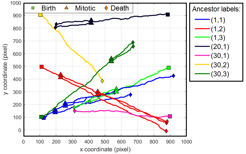
Figure 3: True cell trajectories in simulated detection experiment, each distinct color indicates a family.

Each simulated detection is a vector comprising the 2D position and appearance feature of the cell. These detections are generated with a detection probability of $0.9$, while clutter is uniformly distributed with an average rate of $30$. The appearance feature $\alpha=[\alpha_{1},\alpha_{2}]$ is sampled from Beta distributions. Specifically, if this measurement is generated by: a normal cell then $\alpha_{1}\sim\beta(0.9,0.1)$ and $\alpha_{2}\sim\beta(0.2,0.1)$; a mitotic cell then $\alpha_{1}\sim\beta(0.2,0.1)$ and $\alpha_{2}\sim\beta(0.9,0.1)$. If it is a clutter object then $\alpha_{1}\sim\beta(0.4,0.1)$ and $\alpha_{2}\sim\beta(0.1,0.1)$. The mode likelihood is given as $g^{(a)}(\alpha|1)=\alpha_{1}$ and $g^{(a)}(\alpha|2)=\alpha_{2}$.

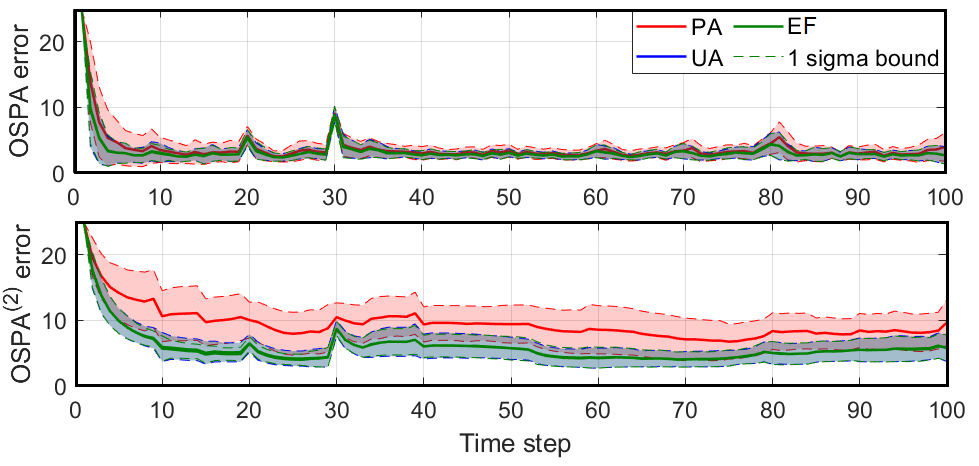
Figure 4: Mean OSPA and $\textrm{OSPA}^{\textrm{(2)}}$ errors in simulated detection experiment.

For the purposes of benchmarking the prediction approximation (PA) and update approximation (UA) against the very expensive implementation of the exact filter (EF), we assume the clutter rate and detection probability are known (whereas these are unknown to the trackers in the next two experiments). All filtering strategies are performed with a component weight threshold of $10^{-5},$a requested number of 30000 solutions from the Gibbs sampler, and a maximum number of 30000 components retained. The mean OSPA and $\textrm{OSPA}^{\textrm{(2)}}$ [51] errors over 100 Monte Carlo (MC) trials shown in Fig. 4. The norm-order and cut-off of the OSPA metrics are set to 1 and 25, respectively (as in [4]), and the window length for $\textrm{OSPA}^{\textrm{(2)}}$ is set to 20 time steps. The OSPA errors for the PA, UA and EF are similar due to the fact that the OSPA does not capture labeling errors. This is confirmed by the $\textrm{OSPA}^{\textrm{(2)}}$ which shows that the UA and EF incur a much lower tracking error than the PA, and can be attributed to more accurate estimation of mitotic events as shown in Fig. 5. The error curves for UA and EF are almost identical which shows that UA is a good approximation of the exact solution.

It can be seen from Fig. 6 that the PA, UA and EF correctly estimate the number of cells, but that the UA and EF exhibit a much lower estimation uncertainty. It further shows that PA slightly overestimates the number of mitotic events. Due to the relatively small number of cells, the PA and UA have approximately similar run times while EF takes significantly longer (more than three times).

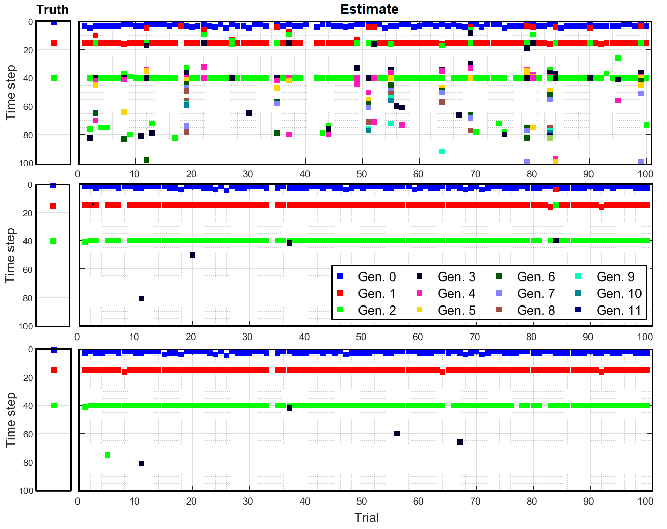
Figure 5: Lineage estimation for one cell family (top: PA, middle: UA, bottom: EF), similar trends are also observed for other families.

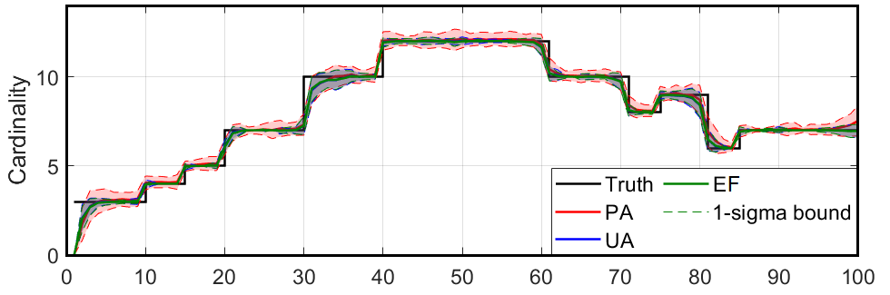
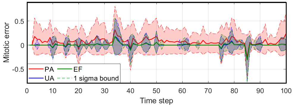
Figure 6: Mean estimated cell cardinality (top) and error in mitotic event counts (bottom) (positive: overestimation, negative: underestimation) in simulated detection experiment.

V-B Synthetic Cells Migration Sequences

In this experiment, cells initially appear randomly with cardinality sampled from a Poisson distribution and locations sampled uniformly within the image. The parameters used to generate the true cell trajectories are given in Tab. III. Parameters for the kinematic model are $w_{1}=0.3$ and $w_{2}=0.7$. Parameters for the mitosis model are $N=9$, $\hat{\theta}=0^{\circ}$, and $\epsilon=20^{\circ}$. Instead of detection sequences, the method in [65] is used to generate 5 different scenarios, containing fluorescent image sequences of cell nucleii, and each with a different level of Charge-Coupled Device noise. Mitotic cells appear with maximum intensity and with a highly eccentric appearance in mimicking a common characteristic in the cell division process. Snapshots for scenarios 1 and 5 are given in Fig. 7. From each of the generated image sequences, the detector proposed in [35] is used to extract cell centroids. Based on a distance limit of 5 pixels around the ground truths, the actual true and false positive rates are tabulated in Tab. IV. The intensity of each detected spot is used as the observed feature of the cell. The likelihood for the intensity is mode dependent, and $g^{(a)}(\cdot|1)$ is designed such that its output is high when the intensity is low, while $g^{(a)}(\cdot|2)$, is high when the intensity is high.

TABLE III: Parameters for true cell trajectories generation in synthetic migration experiment.

Parameters	Values
Initial number of cells	20
Sequence length	100
Image size	$1000\times 1000$
Poisson rate of birth events	0.1
Probability of death events	0.01
Probability of mitotic events	0.05
DM/FD switching probability	0.3/0.7
Uncertainty of free diffusive motion	10 pixels

Figure 7: Snapshots of the synthetic migration sequence at time step 100 (left: scenario 1, right: scenario 5).

TABLE IV: True/False positive rates of the detection in synthetic experiment.

	Scen. 1	Scen. 2	Scen. 3	Scen. 4	Scen. 5
True Pos. Rate	0.8473	0.7752	0.5727	0.4566	0.3862
False Pos. Rate	0	0.97	20.6	62.78	105.72

The same filter settings as the previous experiment are used. However, our filters assume no knowledge of clutter rate and detection parameters. The unknown detection probability is modeled as a Beta distribution as per [52]. For unknown clutter rate estimation [53], the clutter birth rate is set to 0.5 while the clutter surviving and detection rates are set to 0.9 for all scenarios. Due to the large number of cells, the EF becomes intractable as it is intensive in both memory and computations.

Fig. 8 shows that both PA and UA accurately estimate the number of cells in scenarios 1 to 4 but exhibits overestimation in scenario 5 due to the high clutter rate. Fig. 9 shows that the average estimated detection probability decreases across time from scenario 1 to 5. This is due to the difficulty in detection when the cell density increases. The plots of clutter cardinality in Fig. 10 corroborate the average false positive rates shown in Tab. 9. To provide further insight on the estimated detection probability, we show the histograms of cell detection probability across all time steps for all 5 scenarios in Fig. 11. Note that the detection probability of a cell is dependent on its state. Hence, more cells with low detection probability are estimated across different scenarios as seen in Fig. 11, even though Fig. 9 does not show significant reduction in average estimated detection probability. Tab. V shows PA has slightly higher mitotic error compared to UA.

Figure 8: Cell cardinality in synthetic migration experiment (top: PA, bottom: UA).

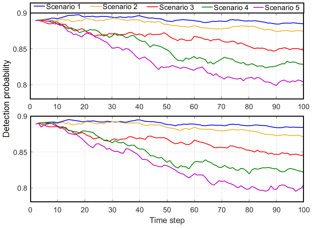
Figure 9: Average estimated cell detection probability in synthetic migration experiment (top: PA, bottom: UA).

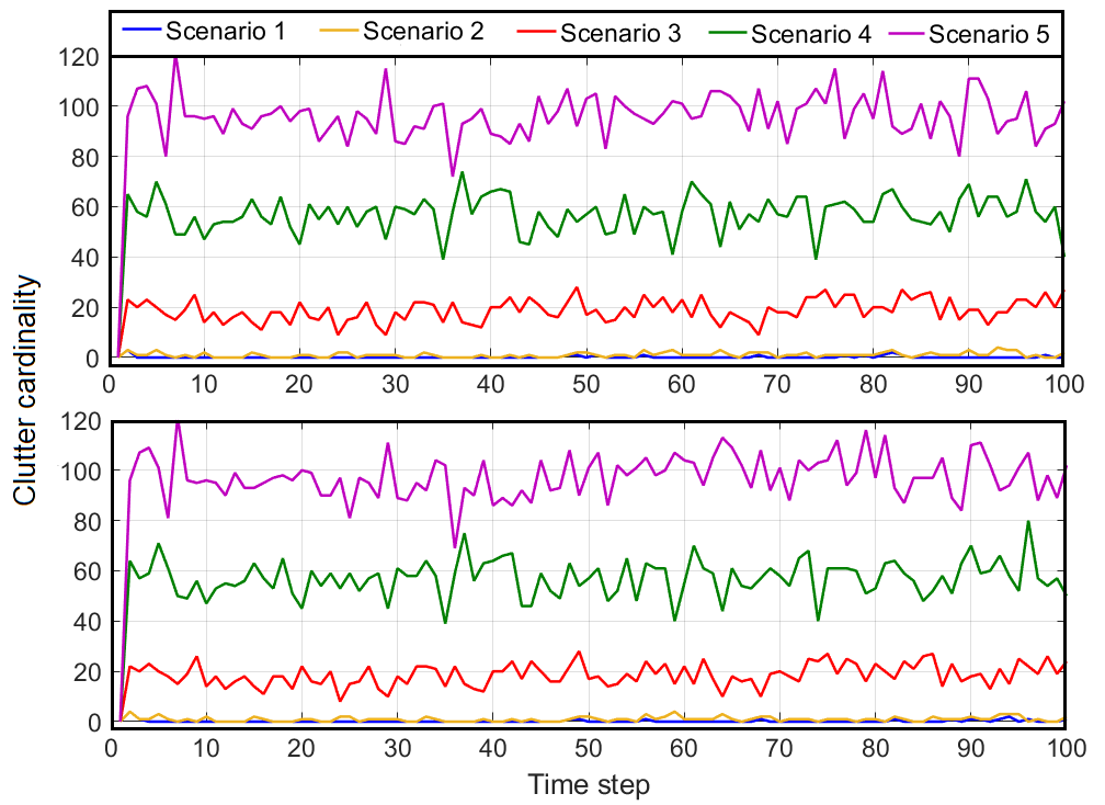
Figure 10: Estimated clutter cardinality in synthetic migration experiment (top: PA, bottom: UA).

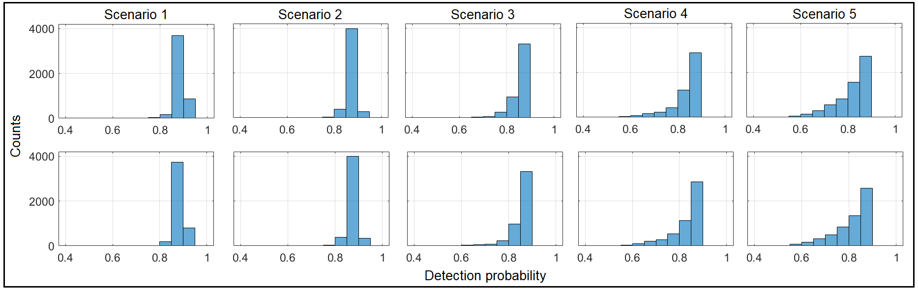
Figure 11: Histograms of cell detection probability (for all time steps) in synthetic migration experiment (top: PA, bottom: UA).

TABLE V: The time-averaged error of estimated mitotic events counts.

	Scen. 1	Scen. 2	Scen. 3	Scen. 4	Scen. 5
PA	1.62	1.53	1.47	1.40	1.23
UA	1.54	1.49	1.43	1.36	1.58

We also provide a performance comparison with other state-of-the-art methods: MHT [4] via icy^© [66] (icy-MHT), global optimization with Viterbi linking algorithm [32] via BaxterAlgorithm [67] (Viterbi Linking), JPDA with Interacting Multiple Models (IMM-JPDA) [49], and Linear Assignment Problem (LAP) via CellProfiler^© [6] (CellProfiler-LAP). The motion model parameters are the same as per our proposed algorithm. Other parameters are taken from actual values in Tab. IV or tuned via the parameters estimation routines provided with the software, prior to tracking.

The $\textrm{OSPA}^{\textrm{(2)}}$ errors over the entire scenario for all filters under consideration are plotted in Fig. 12. It can be seen that the proposed GLMB-based methods have the lowest error, keeping in mind that they have no knowledge of the false positive and negative rates. The errors for the other algorithms are similar in all scenarios, and is highest for CellProfiler-LAP in scenarios 1, 2, 4 and 5, and highest for icy-MHT in scenario 3. The true number of distinct tracks in this experiment is 357. Icy-MHT and Viterbi Linking algorithms overestimate the number of tracks while IMM-JPDA and Cellprofilter-LAP underestimate. On the other hand, our methods yield the lowest error in the number of tracks across all scenarios.

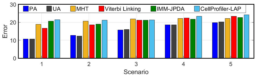
Figure 12: $\textrm{OSPA}^{\textrm{(2)}}$ error (lower is better) of different cell tracking methods across all scenarios in synthetic migration experiment (evaluated over the entire tracking period).

In addition to the $\textrm{OSPA}^{\textrm{(2)}}$ metric, we report the TRA score [68] to evaluate lineage estimation (IMM-JPDA is excluded as it does not provide lineage). Instead of computing the overlap region between the true and the computed cells, we use the Euclidean distance between them as the matching cost. Matches that have distances lower than 25 pixels are counted as true positives. The standard computation for TRA scores then gives the false positives, false negatives links etc. Equal weights are used for all 5 types of errors (merged, false negatives, false positives, false negative links, false positive links and incorrect semantic links). Readers are referred to [68] for more details on TRA score.

The results in Tab. VI indicate that PA has the best performance in TRA score on all scenarios while UA is the second best in scenarios 1 to 4. MHT performs poorly in the 3 most challenging scenarios with a high amount of false tracks which is presumably due to the high clutter rate.

TABLE VI: TRA scores (higher is better) for different algorithms.

	Scen. 1	Scen. 2	Scen. 3	Scen. 4	Scen. 5
PA	0.7458	0.7429	0.6319	0.3295	0.1413
UA	0.7447	0.7331	0.5812	0.3138	0.0678
icy-MHT	0.5584	0.1675	0	0	0
Viterbi Linking	0.5789	0.4763	0.2273	0.1575	0.0811
CellProfiler-LAP	0.4821	0.4694	0.4094	0.0044	0

We compare the computation times of PA and UA (on a 12-core machine at 1.5 GHz with parallelization applied where possible) in Tab. VII noting that both approximate filters exhibit similar performance. The difference in computation times for PA and UA is not significant in the first 2 scenarios but the gaps noticeably widened from scenario 3 onward. Other methods took roughly 5 to 15 minutes to compute the sequences. The additional computation times for the proposed methods is due to the fact it jointly estimates the detection probability and clutter rate whereas the existing methods require these parameters to be known prior to tracking. While these execution times are only meant to be indicative, they suggest that all methods are suitable for live image experiments, which typically have observation intervals of 10-15 minutes.

TABLE VII: Computation times of proposed filters across different scenarios.

	Scen. 1	Scen. 2	Scen. 3	Scen. 4	Scen. 5
PA (min)	20	18	22	38	66
UA (min)	24	25	89	131	187

V-C Breast Cancer Cells Migration Sequence

This experiment considers a real breast cancer cell (MDA-MB-231) dataset in an 88 frame migration sequence of time-lapsed images taken every 15 minutes by inverted microscope. Cell detections are extracted from the images via a neural network called FRCNN-ResNet101 [69] and trained on a separate set of images of the same type of cell. Since mitotic cells have different features to normal cells, we use the output of the last fully-connected layer of FRCNN-ResNet101 to capture their features (1000-dimensional vectors). Specifically, we feed the training sub-images (bounding boxes) of mitotic and normal cells to FRCNN-ResNet101, and then extract the feature vectors from the last fully-connected layer to form $\mathbb{F}_{1}$ (the set of feature vectors of normal cells) and $\mathbb{F}_{2}$ (the set of feature vectors of mitotic cells). To obtain each appearance measurement, we extract the centroid of the box (used as the detected location $\varrho$ of the cell), and then feed the sub-image of the detected cell to FRCNN-ResNet101 to generate $\alpha$.

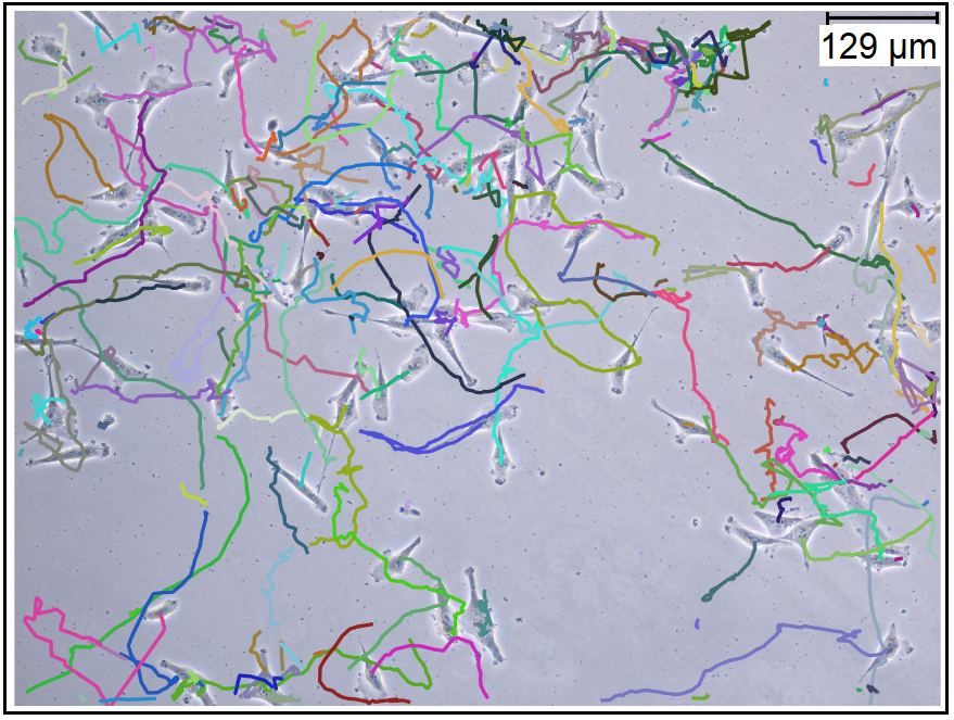
Figure 13: Estimated breast cancer cell trajectories.

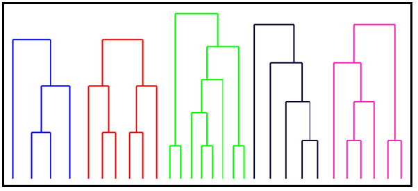
Figure 14: Estimated cell lineages of 5 largest breast cancer cell families, each distinct color indicates a cell family.

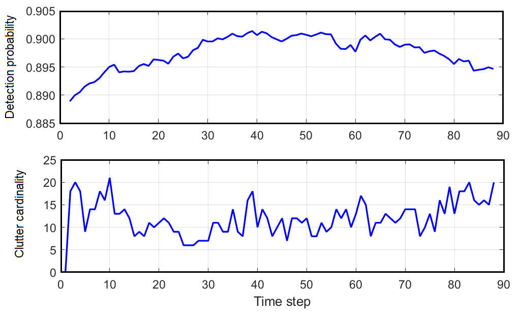
Figure 15: Average estimated detection probability (top) and clutter cardinality (bottom) for breast cancer cells.

Due to the more challenging setting of this experiment, i.e. relatively large number of cells with high uncertainty in dynamic and measurements, we only apply the proposed PA filter. The same dynamic and observation model parameters as in the synthetic data experiments are used, except for the mode likelihood, which is given by $g^{(a)}(\alpha|i)\!\!=\sum_{F\in\mathbb{F}_{i}}\left\|\alpha-F\right\|/\left|\mathbb{F}_{i}\right|$for $i=1,2.$ The filter parameters are also the same as in the synthetic data experiments, except that the number of maximum components is increased to 50000. Fig. 13 shows the trajectories of the estimated cells at the end of the sequence. Fig. 14 also illustrates the estimated cell lineage of the 5 largest cell families. The results demonstrate the capability of the proposed algorithm in tracing cells and their lineages over long periods of time. Fig. 15 shows the average estimated detection probability and clutter cardinality across different time steps.

From the posterior statistics on the population size and mitotic events in Fig. 16, observe that the number of cells increases from approximately 30 in the first frame to nearly 80 in the last frames. Moreover, the relatively tight 1-sigma bounds suggest that the algorithm has high confidence on the estimated cardinality statistics. Fig. 17 shows heat maps of cell concentration in the position and velocity spaces, computed by averaging the intensity function (or probability hypothesis density) over the entire period. Such plots can provide valuable insights into the cell population, such as the regions where cells are more likely to exist (bright spots), or the overall directional drift of cells (in this case slightly downward). Interestingly, the observed cell concentration in the velocity space has a distinctly Gaussian profile.

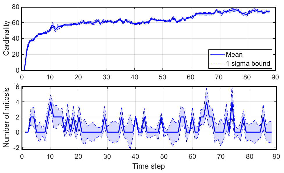
Figure 16: Cardinality and mitotic events counts for breast cancer cells.

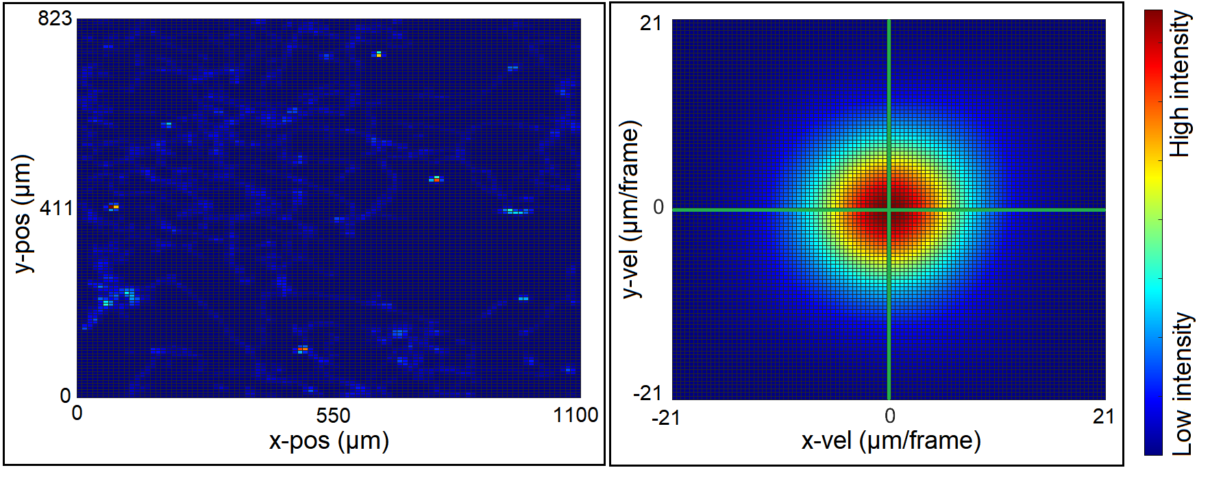
Figure 17: Cell intensity or concentration in position space and velocity space for breast cancer cells.

VI Conclusions

We have proposed labeled RFS solutions for tracking cell trajectories and their lineages. These solutions are based on: a spawning model that takes into account cell lineage and changes in cell appearance prior to division; and multi-object tracking filters for this spawning model. Additionally, the proposed solutions offer the tools for characterizing uncertainty on inferred results, and operate in environments with unknown detection probability and the clutter rate, which is invariably the case in cell experiments. The numerical case studies demonstrate the capability of the proposed solutions to reliably estimate the cell tracks and their lineages. The synthetic data case study, with different level of tracking difficulty, demonstrates significant improvements over existing methods. The real data case study with breast cancer cells migration illustrates the capability to characterize uncertainty on inferred results in providing insightful statistics on the migration of the cell population.

VII Appendix

VII-A Proof of Proposition 1

Substuting (8) to (4) yields

$${\textstyle\boldsymbol{\pi}_{+}\!\left(\boldsymbol{X}_{+}\right)=\boldsymbol{f}_{B,+}(\boldsymbol{B})\int}\boldsymbol{f}_{G,+}(\boldsymbol{Y}|\boldsymbol{X})\boldsymbol{\pi}\left(\boldsymbol{X}\right)\delta\boldsymbol{X},$$ (60)

where $\boldsymbol{Y}$ =$\boldsymbol{X}_{+}-(\mathbb{X}\times\mathbb{B}_{+})$ and $\boldsymbol{B}$ =$\boldsymbol{X}_{+}\cap(\mathbb{X}\times\mathbb{B}_{+})$.

The integral term can be written as

$$\!\!\!\!\!\!\!\!\!\!\!\!\!\!\!\!\int\Delta(\boldsymbol{X})\sum_{I,\xi}\!\omega^{(I,\xi)}\delta_{I}[\mathcal{L}(\boldsymbol{X})]p^{(\xi)}(\boldsymbol{X})\boldsymbol{f}_{+}^{(G)}(\boldsymbol{Y}|\boldsymbol{X})\delta\boldsymbol{X}$$

$$= \!\!\!\!\Delta(\boldsymbol{Y})\sum_{L\subseteq\mathbb{L}}\sum_{I,\xi}\omega^{(I,\xi)}\delta_{I}[L]\eta_{G,+}^{(L,\xi)}(\mathcal{L}(\boldsymbol{Y}))p_{G,+}^{(L,\xi)}(\boldsymbol{Y})$$

$$= \!\!\!\!\Delta(\boldsymbol{Y})\sum_{I,\xi}\!\omega^{(I,\xi)}\eta_{G,+}^{(I,\xi)}(\mathcal{L}(\boldsymbol{Y}))p_{G,+}^{(I,\xi)}(\boldsymbol{Y}).$$

The second line follows from Lemma 7 of [70]. The sum over $L$ vanishes for $L\neq I$, yielding the last line. Further, we replace $\eta_{G,+}^{(I,\xi)}(L)$ by $\sum_{J\subseteq\mathbb{G}_{+}(\mathbb{L})}\delta_{J}(L)\eta_{G,+}^{(I,\xi)}(J)$, and noting that the weights of the LMB birth model (10) can be rewritten as $w_{B,+}(L)=\sum_{J^{\prime}\subseteq\mathbb{B}_{+}}\delta_{J^{\prime}}(L)w_{B,+}(J^{\prime})$, (60) becomes

$$\boldsymbol{\pi}_{+}(\boldsymbol{X}_{+})\!\!\!\!\! = \!\!\!\!\Delta(\boldsymbol{Y})\Delta(\boldsymbol{B})\!\sum_{I,\xi}\!\sum_{J\subseteq\mathbb{G}_{+}(\mathbb{L})}\omega^{(I,\xi)}\delta_{J}[\mathcal{L}(\boldsymbol{Y})]\eta_{G,+}^{(I,\xi)}(J)$$

$$\!\!\!\!\times p_{G,+}^{(I,\xi)}(\boldsymbol{Y})\sum_{J^{\prime}\subseteq\mathbb{B}_{+}}\delta_{J^{\prime}}[\mathcal{L}(\boldsymbol{B})]w_{B,+}(J^{\prime})[p_{B,+}]^{\boldsymbol{B}}$$

$$= \!\!\!\!\Delta(\boldsymbol{X}_{+})\sum_{I,\xi}\sum_{(J\uplus J^{\prime})\subseteq(\mathbb{G}_{+}(\mathbb{L})\uplus\mathbb{B}_{+})}\!\!\delta_{J\uplus J^{\prime}}[\mathcal{L}(\boldsymbol{Y})\uplus\mathcal{L}(\boldsymbol{B})]$$

$$\!\!\!\!\times\omega^{(I,\xi)}w_{B,+}(J^{\prime})\eta_{G,+}^{(I,\xi)}(J)[p_{B,+}]^{\boldsymbol{B}}p_{G,+}^{(I,\xi)}(\boldsymbol{Y})$$

$$= \!\!\!\!\Delta(\boldsymbol{X}_{+})\sum_{I,\xi,I_{+}}\omega^{(I,\xi)}w_{B,+}(I_{+}\cap\mathbb{B}_{+})\times$$

$$\!\!\!\!\eta_{G,+}^{(I,\xi)}(I_{+}-\mathbb{B}_{+})\delta_{I_{+}}[\mathcal{L}(\boldsymbol{X}_{\!+})][p_{B,+}]^{\boldsymbol{B}}p_{G,+}^{(I,\xi)}(\boldsymbol{Y}).$$

The second equation follows from $\boldsymbol{X}_{+}=\boldsymbol{Y}\uplus\boldsymbol{B}$ and $\Delta(\boldsymbol{X}_{+})=\Delta(\boldsymbol{Y})\Delta(\boldsymbol{B})$. The last equation is obtained by substituting $I_{+}$= $J\uplus J^{\prime}$, and $\mathbb{L}_{+}=\mathbb{G}_{+}(\mathbb{L})\uplus\mathbb{B}_{+}$. $\boldsymbol{\enskip\blacksquare}$

VII-B Proof of Proposition 2

Substituting $\boldsymbol{Y}=\boldsymbol{X}_{+}-\mathbb{X}\times\mathbb{B}_{+}$ and $\boldsymbol{B}=\boldsymbol{X}_{+}\cap\mathbb{X}\times\mathbb{B}_{+}$ into (32) gives

$$\boldsymbol{\pi}_{\!+}\!(\boldsymbol{X}_{\!+})\!\!\!\!\! = \!\!\!\!\Delta(\boldsymbol{X}_{\!+})\!\!\sum_{I,\xi,I_{+}}\!\!\omega_{+}^{(I,\xi,I_{+\!})}\delta_{I_{+\!}}[\mathcal{L}(\boldsymbol{X}_{\!+})]\left[p_{B,+}\right]{}^{\boldsymbol{B}}p_{G,+}^{(I,\xi)}(\boldsymbol{Y}).$$

Applying Bayes rule, we have

$$\boldsymbol{\pi}_{\!+}\!(\boldsymbol{X}_{\!+}|Z_{+})\!\!\!\! \propto \!\!\!\!\Delta(\boldsymbol{X}_{\!+})\!\!\sum_{I,\xi,I_{+}}\!\!\omega_{+}^{(I,\xi,I_{+\!})}\delta_{I_{+\!}}[\mathcal{L}(\boldsymbol{X}_{\!+})]\left[p_{B,+}\right]{}^{\boldsymbol{B}}$$

$$\!\!\!\!p_{G,+}^{(I,\xi)}(\boldsymbol{Y})\sum_{\theta_{+}\in\Theta_{+}}1_{\Theta_{+}(\mathcal{L}(\boldsymbol{X}_{+}))}(\theta_{+})[\varPsi_{Z_{+}}^{(\theta_{+})}]^{\boldsymbol{X}_{+}}.$$

Further, substituting $[\varPsi_{Z_{+}}^{(\theta_{+})}]^{\boldsymbol{X}_{+}}$ = $[\varPsi_{Z_{+}}^{(\theta_{+})}]^{\boldsymbol{B}}[\varPsi_{Z_{+}}^{(\theta_{+})}]^{\boldsymbol{Y}}$ and $I_{+}=\mathcal{L}(\boldsymbol{X}_{+})$ yields

$$\boldsymbol{\pi}_{\!+}\!(\boldsymbol{X}_{\!+}|Z_{+})\propto\Delta(\boldsymbol{X}_{\!+})\!\!\sum_{I,\xi,I_{+},\theta_{+}}\!\omega_{+}^{(I,\xi,I_{+\!})}\delta_{I_{+\!}}[\mathcal{L}(\boldsymbol{X}_{\!+})]\!\times\\ 1_{\Theta_{+}(I_{+})}(\theta_{+})\left[p_{B,+}\varPsi_{Z_{+}}^{(\theta_{+})}\right]{}^{\boldsymbol{B}}p_{G,+}^{(I,\xi)}(\boldsymbol{Y})[\varPsi_{Z_{+}}^{(\theta_{+})}]^{\boldsymbol{Y}}\\ =\Delta(\boldsymbol{X}_{\!+})\!\!\sum_{I,\xi,I_{+},\theta_{+}}\!\!\omega_{+}^{(I,\xi,I_{+\!})}1_{\Theta_{+}(I_{+})}(\theta_{+})\delta_{I_{+\!}}[\mathcal{L}(\boldsymbol{X}_{\!+})]\times\\ \!\left[\eta_{B,Z_{+}}^{(\theta_{+})}\right]^{\mathcal{L}(\boldsymbol{B})}\eta_{G,Z_{+}}^{(I,\xi,\theta_{+})}(\mathcal{L}(\boldsymbol{Y}))\left[p_{B,Z_{+}}^{(\theta_{+})}\!\right]\!^{\!\boldsymbol{B}}p_{G,Z_{+}}^{(I,\xi,\theta_{+})}(\boldsymbol{Y}).\enskip\blacksquare$$

VII-C Equivalence of (36) and (46)

Expanding (36) we have

$$\tilde{\omega}{}_{Z_{+}}^{(I,\xi,I_{+},\theta_{+})}=\omega^{(I,\xi)}w_{B,+}(I_{+}\cap\mathbb{B}_{+})\eta_{G,+}^{(I,\xi))}(I_{+}-\mathbb{B}_{+})\times\\ 1_{\Theta_{+}(I_{+})}(\theta_{+})\left[\eta_{B,Z_{+}}^{(\theta_{+})}\right]^{I_{+}\cap\mathbb{B}_{+}}\left[\tilde{\eta}_{G,Z_{+}}^{(I,\xi,I_{+},\theta_{+})}\right]^{(I_{+}-\mathbb{B}_{+})}.$$

For the birth terms, we write

$$w_{B,+}(I_{+}\cap\mathbb{B}_{+}) \!\!\!\!=\!\!\!\! [1-r_{B,+}(\cdot)]^{\mathbb{B}_{+}-I_{+}}[r_{B,+}(\cdot)]^{I_{+}\cap\mathbb{B}_{+}},$$

$$\left[\eta_{B,Z_{+}}^{(\theta_{+})}\right]^{I_{+}\cap\mathbb{B}_{+}} \!\!\!\!=\!\!\!\! \left[\int p_{+}^{(B)}(x_{+},\cdot)\psi_{Z_{+}}^{(\theta_{+}(\cdot))}(x_{+},\cdot)dx_{+}\right]^{I_{+}\cap\mathbb{B}_{+}}.$$

For the survival terms we write

$$\eta_{G,+}^{(I,\xi)}(I_{+}-\mathbb{B}_{+})\!=\! \left\langle\prod_{\ell\in I}q_{G,+}^{(\ell,\xi)}((I_{+}-\mathbb{B}_{+})\!\cap\!\mathbb{G}_{+}(\ell))\right\rangle\!(I_{+}-\mathbb{B}_{+})$$

$$=\! \prod_{\ell\in I}\left\langle q_{G,+}^{(\ell,\xi)}(I_{+}\cap\mathbb{G}_{+}(\ell))\right\rangle(I_{+}\cap\mathbb{G}_{+}(\ell))$$

$$=\! \prod_{\ell\in I}\eta_{G,+}^{(\ell,\xi)}(I_{+}\cap\mathbb{G}_{+}(\ell)),$$

where the second equation follows from the separation of independent variables for integration, and

$$\!\!\!\!\!\!\!\![\tilde{\eta}_{G,Z_{+}}^{(I,\xi,I_{+},\theta_{+})}]^{(I_{+}-\mathbb{B}_{+})}\!=\!\!\!\!\prod_{u\in I_{+}-\mathbb{B}_{+}}\left\langle p_{G,+}^{(I,\xi,I_{+}-\mathbb{B}_{+})}(\cdot,u),\varPsi_{Z_{+}}^{(\theta_{+})}(\cdot,u)\right\rangle\\ =\prod_{\ell\in I}\prod_{\ell_{+}\in I_{+}\cap\mathbb{G}_{+}(\ell)}\left\langle p_{G,+}^{(\ell,\xi,I_{+}\cap\mathbb{G}_{+}(\ell))}(\cdot,\ell_{+}),\varPsi_{Z_{+}}^{(\theta_{+})}(\cdot,\ell_{+})\right\rangle.$$

Grouping the appropriate terms yields (46).$\enskip\blacksquare$

VIII Proof of Proposition 6

It suffices to show that

$$\pi_{n}(\gamma_{n}|\gamma_{\bar{n}}) \propto\lambda_{n}^{(I,\xi)}(\gamma_{n})\prod_{i\in\bar{n}}\Upsilon_{\{1:M\}}(\gamma_{n},\gamma_{i}),$$ (61)

where

$$\Upsilon_{\{1:M\}}(\gamma_{n},\gamma_{i})=\prod_{(q,r)=(1,1)}^{(3,3)}(1-1_{\{1:M\}}(\gamma_{n,q})\delta_{\gamma_{n,q}}[\gamma_{i,r}]).$$

To prove (61), we first show that $1_{\Gamma}(\gamma)$ can be written in the following product form

$$1_{\Gamma}(\gamma) =1_{\Gamma(\bar{n})}(\gamma_{\bar{n}})\prod_{i\in\bar{n}}\Upsilon_{\{1:M\}}(\gamma_{n},\gamma_{i}),$$ (62)

where $\Gamma(\bar{n})$ is the set of all 1-1 positive $\gamma_{\bar{n}}$.

For $n\in\{1:P\}$, since $\gamma_{n}\in\mathbb{D}_{+}\uplus\mathbb{N}_{+}$ the positive 1-1 condition is guaranteed by the definition of $\lambda_{n}^{(I,\xi)}$. It remains to prove that if $\prod_{i\in\bar{n}}\Upsilon_{\{1:M\}}(\gamma_{n},\gamma_{i})=1$ then $\gamma$ is positive 1-1.

To prove (62), we will show that: (a) if $\gamma$ is positive 1-1 then RHS of (62) equates to 1; and (b) if $\gamma$ is not positive 1-1 then RHS of (62) equates to 0.

For (a), assume that $\gamma$ is positive 1-1, then for any $i\neq j\in\bar{n}$, $\Upsilon_{\{1:M\}}(\gamma_{j},\gamma_{i})=1$ hence RHS equates to 1. For (b), assume that $\gamma$ is not positive 1-1, if $\gamma_{\bar{n}}$ is also not positive 1-1, hence there exists $i\neq j\in\bar{n}$ such that $\Upsilon_{\{1:M\}}(\gamma_{j},\gamma_{i})=0$ hence $1_{\Gamma(\bar{n})}(\gamma_{\bar{n}})=0$, hence RHS equates to 0. If $\gamma_{\bar{n}}$ is positive 1-1, as $\gamma$ is not positive 1-1, hence there exists $i$ and $j$ such that $\Upsilon_{\{1:M\}}(\gamma_{j},\gamma_{i})=0$. Either $i$ or $j$ has to equal $n$ as the 1-1 positive of $\gamma_{\bar{n}}$ are in $\bar{n}$ then we have a contradiction. Hence the RHS must equate to 0. To prove (61), as we are interested in the relationship between $\pi_{n}(\gamma_{n}|\gamma_{\bar{n}})$ and $\gamma_{n}$, we can write

$$\pi_{n}(\gamma_{n}|\gamma_{\bar{n}})\propto\pi(\gamma)\propto 1_{\Gamma}(\gamma)\prod_{j=1}^{P}\lambda_{i}^{(I,\xi)}(\gamma_{j}).$$

Applying (62) to the above expression yields

$$\pi_{n}(\gamma_{n}|\gamma_{\bar{n}})\\ \propto\lambda_{n}^{(I,\xi)}(\gamma_{n})\prod_{i\in\bar{n}}\Upsilon_{\{1:M\}}(\gamma_{n},\gamma_{i})1_{\Gamma(\bar{n})}(\gamma_{\bar{n}})\prod_{j\in\bar{n}}\lambda_{j}^{(I,\xi)}(\gamma_{j})\\ \propto\lambda_{n}^{(I,\xi)}(\gamma_{n})\prod_{i\in\bar{n}}\Upsilon_{\{1:M\}}(\gamma_{n},\gamma_{i}).\enskip\blacksquare$$

IX Proof of Proposition 7

Note from the $n^{th}$ conditional given by (61) that $\Upsilon_{\{1:M\}}(\gamma_{n},\gamma_{j})=1$, for each $j\in\{1:n-1\}$. Hence,

$$\!\!\pi_{n}(\gamma^{\prime}_{n}|\gamma^{\prime}_{1:n-1},\gamma{}_{n+1:P}) =\lambda_{n}^{(I,\xi)}(\gamma^{\prime}_{n})\frac{\prod_{j=n+1}^{P}\Upsilon_{\{1:M\}}(\gamma_{n},\gamma_{j})}{K_{n}(\gamma^{\prime}_{1:n-1},\gamma_{n+1:P})},$$

where $K_{n}$ is the normalizing constant in the $n^{th}$ sub-iteration of the block Gibbs sampler. We define $\upsilon_{n}=[-1,-1,0]\otimes[\mathbf{1}_{n}]^{T}$, where $\mathbf{1}_{n}$ is the $n$-dimensional one vector. If $\gamma^{\prime}=\upsilon_{P}$, then for each $j\in\{n+1:P\}$, $\prod_{t=-1}^{0}\prod_{s=1}^{3}(1-1_{\{1:M\}}(\gamma_{j,s})\delta_{t}[\gamma_{j,s}])=1$ as an assignment cannot take -1 or 0 and a positive number at the same time hence

$$\pi_{n}\left(\upsilon_{P}|\gamma^{\prime}_{1:n-1},\gamma{}_{n+1:P}\right) =\prod_{n=1}^{P}\frac{\lambda_{n}^{(I,\xi)}\left(\upsilon_{1}\right)}{K_{n}\left(\upsilon_{n-1},\gamma_{n+1:P}\right)}>0,$$

if $\gamma=\upsilon_{P}$ then $1_{\{1:M\}}(\gamma_{j,r})=0$ for $r\in\{1,2,3\}$, hence

$$\pi_{n}(\gamma^{\prime}_{n}|\upsilon_{P}) =\prod_{n=1}^{P}\frac{\lambda_{n}^{(I,\xi)}(\gamma^{\prime}_{n})}{K_{n}\left(\gamma^{\prime}_{n},\upsilon_{P-n}\right)}>0.$$

Hence, the 2-step probability transition is

$$\pi^{2}(\gamma^{\prime}|\gamma)=\sum_{\varsigma\in\Gamma}\pi(\gamma^{\prime}|\varsigma)\pi(\varsigma|\gamma^{\prime})>\\ \pi_{n}\left(\gamma^{\prime}_{n}|\upsilon_{P}\right)\pi_{n}\left(\upsilon_{P}|\gamma^{\prime}_{1:n-1},\gamma{}_{n+1:P}\right)>0.$$

This condition is sufficient for the block Gibbs sampler to converge to the target distribution (Proposition 4 in [60]). $\boldsymbol{\enskip\blacksquare}$

References

- [1] M. A. A. Dewan, M. O. Ahmad, and M. N. S. Swamy, “Tracking biological cells in time-lapse microscopy: An adaptive technique combining motion and topological features,” IEEE Trans. Biomed. Eng., vol. 58, no. 6, pp. 1637–1647, 2011.
- [2] S. G. Megason and S. E. Fraser, “Imaging in systems biology,” Cell, vol. 130, no. 5, pp. 784–795, 2007.
- [3] R. Hoseinnezhad, B.-N. Vo, B.-T. Vo, and D. Suter, “Visual tracking of numerous targets via multi-Bernoulli filtering of image data,” Pattern Recognition, vol. 45, no. 10, pp. 3625–3635, 2012.
- [4] N. Chenouard, I. Bloch, and J. Olivo-Marin, “Multiple hypothesis tracking for cluttered biological image sequences,” IEEE Trans. Pattern Anal. Mach. Intell., vol. 35, no. 11, pp. 2736–3750, 2013.
- [5] S. H. Rezatofighi, S. Gould, B.-T. Vo, B.-N. Vo, K. Mele, and R. Hartley, “Multi-target tracking with time-varying clutter rate and detection profile: Application to time-lapse cell microscopy sequences,” IEEE Trans. Med. Imag., vol. 34, no. 6, pp. 1336–1348, 2015.
- [6] A. Carpenter et al., “CellProfiler: Image analysis software for identifying and quantifying cell phenotypes,” Genome biology, vol. 7, p. R100, 02 2006.
- [7] I. Smal, K. Draegestein, N. Galjart, W. Niessen, and E. Meijering, “Particle filtering for multiple object tracking in dynamic fluorescence microscopy images: Application to microtubule growth analysis,” IEEE Trans. Med. Imag., vol. 27, no. 6, pp. 789–804, 2008.
- [8] E. Meijering, I. Smal, and G. Danuser, “Tracking in molecular bioimaging,” IEEE Signal Process. Mag., vol. 23, no. 3, pp. 46–53, 2006.
- [9] J. Chen, M. S. Alber, and D. Z. Chen, “A hybrid approach for segmentation and tracking of myxococcus xanthus swarms,” IEEE Trans. Med. Imag., vol. 35, no. 9, pp. 2074–2084, 2016.
- [10] O. Hirose et al., “SPF-CellTracker: Tracking multiple cells with strongly-correlated moves using a spatial particle filter,” IEEE/ACM Trans. Comput. Biol. Bioinformatics, vol. 15, no. 6, pp. 1822–1831, 2018.
- [11] B. Xu, M. Lu, J. Cong, and B. Nener, “An ant colony inspired multi-Bernoulli filter for cell tracking in time-lapse microscopy sequences,” IEEE J. Biomed. Health Inform., pp. 1–1, 2019.
- [12] M. A. Lodato et al., “Somatic mutation in single human neurons tracks developmental and transcriptional history,” Science, vol. 350, no. 6256, pp. 94–98, 2015.
- [13] R. P. S. Mahler, Statistical multisource-multitarget information fusion. Artech House, 2007.
- [14] ——, Advances in statistical multisource-multitarget information fusion. Artech House, 2014.
- [15] B.-N. Vo and B.-T. Vo, “A multi-scan labeled random finite set model for multi-object state estimation,” IEEE Trans. Signal Process., vol. 67, no. 19, pp. 4948–4963, Oct 2019.
- [16] D. Reid, “An algorithm for tracking multiple targets,” IEEE Trans. Autom. Control, vol. 24, no. 6, pp. 843–854, December 1979.
- [17] T. Fortmann, Y. Bar-Shalom, and M. Scheffe, “Sonar tracking of multiple targets using joint probabilistic data association,” IEEE J. Ocean. Eng., vol. 8, no. 3, pp. 173–184, 1983.
- [18] D. Y. Kim, B.-N. Vo, A. Thian, and Y. S. Choi, “A generalized labeled multi-Bernoulli tracker for time lapse cell migration,” in Int. Conf. on Control, Automation and Information Sciences, 2017, pp. 20–25.
- [19] T. T. D. Nguyen and D. Y. Kim, “On-line tracking of cells and their lineage from time lapse video data,” in Int. Conf. on Control, Automation and Information Sciences, 2018, pp. 291–296.
- [20] D. S. Bryant, B.-T. Vo, B.-N. Vo, and B. A. Jones, “A generalized labeled multi-Bernoulli filter with object spawning,” IEEE Trans. Signal Process., vol. 66, no. 23, pp. 6177–6189, Dec 2018.
- [21] B.-T. Vo and B.-N. Vo, “Labeled random finite sets and multi-object conjugate priors,” IEEE Trans. Signal Process., vol. 61, no. 13, pp. 3460–3475, 2013.
- [22] F. Papi, B.-N. Vo, B.-T. Vo, C. Fantacci, and M. Beard, “Generalized labeled multi-Bernoulli approximation of multi-object densities,” IEEE Trans. Signal Process., vol. 63, no. 20, pp. 5487–5497, 2015.
- [23] C.-Y. Lee, S. Kang, A. D. Chisholm, and P. C. Cosman, “Automated cell junction tracking with modified active contours guided by SIFT flow,” in IEEE Int. Symp. on Biomedical Imaging, 2014, pp. 290–293.
- [24] K. Li, E. D. Miller, M. Chen, T. Kanade, L. E. Weiss, and P. G. Campbell, “Cell population tracking and lineage construction with spatiotemporal context,” Medical Image Analysis, vol. 12, no. 5, pp. 546 – 566, 2008.
- [25] D. P. Mukherjee, N. Ray, and S. T. Acton, “Level set analysis for leukocyte detection and tracking,” IEEE Trans. Image Process., vol. 13, no. 4, pp. 562–572, 2004.
- [26] Z. Lu, G. Carneiro, and A. P. Bradley, “An improved joint optimization of multiple level set functions for the segmentation of overlapping cervical cells,” IEEE Trans. Image Process., vol. 24, no. 4, pp. 1261–1272, 2015.
- [27] O. Dzyubachyk, W. A. van Cappellen, J. Essers, W. J. Niessen, and E. Meijering, “Advanced level-set-based cell tracking in time-lapse fluorescence microscopy,” IEEE Trans. Med. Imag., vol. 29, no. 3, pp. 852–867, 2010.
- [28] O. Debeir, P. Van Ham, R. Kiss, and C. Decaestecker, “Tracking of migrating cells under phase-contrast video microscopy with combined mean-shift processes,” IEEE Trans. Med. Imag., vol. 24, no. 6, pp. 697–711, 2005.
- [29] F. Boukari and S. Makrogiannis, “Automated cell tracking using motion prediction-based matching and event handling,” IEEE/ACM Trans. Comput. Biol. Bioinformatics, vol. 17, no. 3, pp. 959–971, 2020.
- [30] E. Turetken, X. Wang, C. J. Becker, C. Haubold, and P. Fua, “Network flow integer programming to track elliptical cells in time-lapse sequences,” IEEE Trans. Med. Imag., vol. 36, no. 4, pp. 942–951, 2017.
- [31] I. Sbalzarini and P. Koumoutsakos, “Feature point tracking and trajectory analysis for video imaging in cell biology,” Journal of Structural Biology, vol. 151, no. 2, pp. 182–195, 2005.
- [32] K. E. G. Magnusson, J. Jalden, P. M. Gilbert, and H. M. Blau, “Global linking of cell tracks using the Viterbi algorithm,” IEEE Trans. Med. Imag., vol. 34, no. 4, pp. 911–929, 2015.
- [33] L. Vincent and P. Soille, “Watersheds in digital spaces: an efficient algorithm based on immersion simulations,” IEEE Trans. Pattern Anal. Mach. Intell., vol. 13, no. 6, pp. 583–598, 1991.
- [34] N. Otsu, “A threshold selection method from gray-level histograms,” IEEE Trans. Syst., Man, Cybern., vol. 9, no. 1, pp. 62–66, 1979.
- [35] S. Rezatofighi, R. Hartley, and W. Hughes, “A new approach for spot detection in total internal reflection fluorescence microscopy,” in IEEE Int. Symp. on Biomedical Imaging, 2012, pp. 860–863.
- [36] J.-C. Olivo-Marin, “Extraction of spots in biological images using multiscale products,” Pattern Recognition, vol. 35, no. 9, pp. 1989 – 1996, 2002.
- [37] O. Ronneberger, P. Fischer, and T. Brox, “U-Net: Convolutional networks for biomedical image segmentation,” in Medical Image Computing and Computer-Assisted Intervention, 2015, pp. 234–241.
- [38] D. Ciresan, A. Giusti, L. M. Gambardella, and J. Schmidhuber, “Deep neural networks segment neuronal membranes in electron microscopy images,” in Advances in Neural Information Processing Systems. Curran Associates, Inc., 2012, pp. 2843–2851.
- [39] C. Ritter, T. Wollmann, J. . Lee, R. Bartenschlager, and K. Rohr, “Deep learning particle detection for probabilistic tracking in fluorescence microscopy images,” in IEEE Int. Symp. on Biomedical Imaging, 2020, pp. 977–980.
- [40] A. Liu, Y. Lu, M. Chen, and Y. Su, “Mitosis detection in phase contrast microscopy image sequences of stem cell populations: A critical review,” IEEE Trans. Big Data, vol. 3, no. 4, pp. 443–457, 2017.
- [41] A. Paul and D. P. Mukherjee, “Mitosis detection for invasive breast cancer grading in histopathological images,” IEEE Trans. Image Process., vol. 24, no. 11, pp. 4041–4054, 2015.
- [42] A. Liu, K. Li, and T. Kanade, “A semi-Markov model for mitosis segmentation in time-lapse phase contrast microscopy image sequences of stem cell populations,” IEEE Trans. Med. Imag., vol. 31, no. 2, pp. 359–369, 2012.
- [43] A. El-Labban, A. Zisserman, Y. Toyoda, A. W. Bird, and A. Hyman, “Discriminative semi-markov models for automated mitotic phase labelling,” in IEEE Int. Symp. on Biomedical Imaging, 2012, pp. 760–763.
- [44] M. Schiegg, P. Hanslovsky, B. X. Kausler, L. Hufnagel, and F. A. Hamprecht, “Conservation tracking,” in IEEE Int. Conf. on Computer Vision, Dec 2013, pp. 2928–2935.
- [45] S. Huh, D. F. E. Ker, R. Bise, M. Chen, and T. Kanade, “Automated mitosis detection of stem cell populations in phase-contrast microscopy images,” IEEE Trans. Med. Imag., vol. 30, no. 3, pp. 586–596, 2011.
- [46] A. Chakraborty and A. K. Roy-Chowdhury, “Context aware spatio-temporal cell tracking in densely packed multilayer tissues,” Medical Image Analysis, vol. 19, no. 1, pp. 149–163, 2015.
- [47] B. Xu, M. Lu, J. Shi, J. Cong, and B. Nener, “A joint tracking approach via ant colony evolution for quantitative cell cycle analysis,” IEEE J. Biomed. Health Inform., vol. 25, no. 6, pp. 2338–2349, 2021.
- [48] K. Thirusittampalam, M. J. Hossain, O. Ghita, and P. F. Whelan, “A novel framework for cellular tracking and mitosis detection in dense phase contrast microscopy images,” IEEE J. Biomed. Health Inform., vol. 17, no. 3, pp. 642–653, 2013.
- [49] S. H. Rezatofighi, A. Milan, Z. Zhang, Q. Shi, A. Dick, and I. Reid, “Joint probabilistic data association revisited,” in Int. Conf. on Computer Vision, 2015, pp. 3047–3055.
- [50] I. Schlangen, J. Franco, J. Houssineau, W. T. E. Pitkeathly, D. Clark, I. Smal, and C. Rickman, “Marker-less stage drift correction in super-resolution microscopy using the single-cluster PHD filter,” IEEE J. Sel. Topics Signal Process., vol. 10, no. 1, pp. 193–202, 2016.
- [51] M. Beard, B.-T. Vo, and B.-N. Vo, “A solution for large-scale multi-object tracking,” IEEE Trans. Signal Process., vol. 68, pp. 2754–2769, 2020.
- [52] R. P. S. Mahler, B.-T. Vo, and B.-N. Vo, “CPHD filtering with unknown clutter rate and detection profile,” IEEE Trans. Signal Process., vol. 59, no. 8, pp. 3497–3513, 2011.
- [53] Y. G. Punchihewa, B.-T. Vo, B.-N. Vo, and D. Y. Kim, “Multiple object tracking in unknown backgrounds with labeled random finite sets,” IEEE Trans. Signal Process., vol. 66, no. 11, pp. 3040–3055, June 2018.
- [54] C.-T. Do and T. T. D. Nguyen, “Multiple marine ships tracking from multistatic Doppler data with unknown clutter rate,” in Int. Conf. on Control, Automation and Information Sciences, 2019, pp. 1–6.
- [55] B.-T. Vo, B.-N. Vo, and A. Cantoni, “Analytic implementations of the cardinalized probability hypothesis density filter,” IEEE Trans. Signal Process., vol. 55, no. 7, pp. 3553–3567, 2007.
- [56] B. Ristic, S. Arulamalam, and N. Gordon, Beyond the Kalman filter. Artech House, 2004.
- [57] B.-N. Vo, S. Singh, and A. Doucet, “Sequential Monte Carlo methods for multi-target filtering with random finite sets,” IEEE Trans. Aerosp. Electron. Syst., vol. 41, no. 4, pp. 1224–1245, 2005.
- [58] B.-N. Vo, B.-T. Vo, and D. Phung, “Labeled random finite sets and the Bayes multi-target tracking filter,” IEEE Trans. Signal Process., vol. 62, no. 24, pp. 6554–6567, 2014.
- [59] T. T. D. Nguyen and D. Y. Kim, “GLMB tracker with partial smoothing,” Sensors, vol. 19, no. 20, 2019.
- [60] B.-N. Vo, B.-T. Vo, and H. G. Hoang, “An efficient implementation of the generalized labeled multi-Bernoulli filter,” IEEE Trans. Signal Process., vol. 65, no. 8, pp. 1975–1987, 2017.
- [61] S. Reuter, B.-T. Vo, B.-N. Vo, and K. Dietmayer, “The labeled multi-Bernoulli filter,” IEEE Trans. Signal Process., vol. 62, no. 12, pp. 3246–3260, 2014.
- [62] K. G. Murty, “An algorithm for ranking all the assignments in order of increasing cost,” Operations Research, vol. 16, no. 3, pp. 682–687, 1968.
- [63] M. L. Miller, H. S. Stone, and I. J. Cox, “Optimizing Murty’s ranked assignment method,” IEEE Trans. Aerosp. Electron. Syst., vol. 33, no. 3, pp. 851–862, July 1997.
- [64] C. R. Pedersen, L. R. Nielsen, and K. A. Andersen, “An algorithm for ranking assignments using reoptimization,” Computers & Operations Research, vol. 35, no. 11, pp. 3714 – 3726, 2008.
- [65] A. Lehmussola, P. Ruusuvuori, J. Selinummi, H. Huttunen, and O. Yli-Harja, “Computational framework for simulating fluorescence microscope images with cell populations,” IEEE Trans. Med. Imag., vol. 26, no. 7, pp. 1010–1016, July 2007.
- [66] Institut Pasteur France-BioImaging, “Icy,” 2.1.0.0.
- [67] K. E. G. Magnusson, “Segmentation and tracking of cells and particles in time-lapse microscopy,” 2016.
- [68] P. Matula, M. Maska, D. V. Sorokin, P. Matula, C. Ortiz-de Solorzano, and M. Kozubek, “Cell tracking accuracy measurement based on comparison of acyclic oriented graphs,” PLOS ONE, vol. 10, no. 12, 2015.
- [69] S. Ren, K. He, R. Girshick, and J. Sun, “Faster R-CNN: Towards real-time object detection with region proposal networks,” IEEE Trans. Pattern Anal. Mach. Intell., vol. 39, no. 6, pp. 1137–1149, Jun 2017.
- [70] M. Beard, B.-T. Vo, and B.-N. Vo, “Bayesian multi-target tracking with merged measurements using labelled random finite sets,” IEEE Trans. Signal Process., vol. 63, no. 6, pp. 1433–1447, 2015.