Distilling Audio-Visual Knowledge by Compositional Contrastive Learning

Abstract

Having access to multi-modal cues (e.g. vision and audio) empowers some cognitive tasks to be done faster compared to learning from a single modality. In this work, we propose to transfer knowledge across heterogeneous modalities, even though these data modalities may not be semantically correlated. Rather than directly aligning the representations of different modalities, we compose audio, image, and video representations across modalities to uncover richer multi-modal knowledge. Our main idea is to learn a compositional embedding that closes the cross-modal semantic gap and captures the task-relevant semantics, which facilitates pulling together representations across modalities by compositional contrastive learning. We establish a new, comprehensive multi-modal distillation benchmark on three video datasets: UCF101, ActivityNet, and VGGSound. Moreover, we demonstrate that our model significantly outperforms a variety of existing knowledge distillation methods in transferring audio-visual knowledge to improve video representation learning. Code is released here: https://github.com/yanbeic/CCL.

1 Introduction

Videos often contain informative multi-modal cues, such as visual objects, motion, auditory events, and textual information encoded in captions or speech – all of which provide rich, transferrable semantics for representation learning. The majority of existing works in video understanding utilises visual-only content for representation learning [63, 52, 57, 64, 10, 19]. Our objective, on the other hand, is to distill the rich multi-modal knowledge available in networks pre-trained on spatial imagery data and temporal auditory data to learn more expressive video representations.

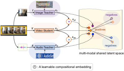
Figure 1: Our generic multi-modal distillation framework aligns audio, image, and video representations in the latent space by compositional contrastive learning, where a compositional embedding is learned to bridge the cross-modal semantic gap and capture the task-relevant semantics for more informative knowledge transfer.

In contrast to the standard knowledge distillation techniques [29, 9] which transfer unimodal knowledge learned from the same modality and dataset, our multi-modal distillation framework uniquely utilises knowledge learned from multiple data modalities. Although prior works have considered cross-modal distillation [24, 6, 3, 34, 2], they generally assume pairwise semantic correspondence between two modalities. However, in unconstrained scenarios, the cross-modal content may not always be semantically correlated or temporally aligned, e.g. a video of applying lipstick, may be accompanied by audio not directly related to the action, such as music or speech. On the other hand, similar audio cues, e.g. music, may accompany videos showing distinct visual content, e.g. applying lipstick and playing cello.

In this work, we tackle a realistic multi-modal distillation paradigm that can distill heterogeneous audio and visual knowledge for video representation learning. This requires to bridge the cross-modal semantic gap, domain gap, as well as dealing with inconsistent network architectures across modalities. To address these challenges in a unified formulation, we propose compositional contrastive learning – a novel, generic framework to distill the multi-modal knowledge by flexibly plugging in the teacher networks pre-trained on different data modalities. Specifically, a compositional embedding is learned to close the cross-modal gap between the teacher and student networks and capture the task-relevant semantics. By jointly pulling together the teacher, student, and their compositional embeddings through compositional contrastive learning, the multi-modal knowledge is transferred to the video student network to learn more powerful video representations.

Our contributions are as follows. (1) We propose a novel Compositional Contrastive Learning (CCL) model, featured by learnable compositional embeddings that close the cross-modal semantic gap, and a distillation objective which contrasts different modalities jointly in the shared latent space, where class labels are introduced to distill the multi-modal knowledge in an informative way. (2) We establish a new benchmark on multi-modal distillation, comparing CCL extensively to seven state-of-the-art distillation methods on three video datasets: UCF101, ActivityNet, VGGSound, in two tasks: video recognition and video retrieval. (3) We demonstrate the advantages of our model in comparison to the prior state-of-the-art methods, and provide an insightful quantitative and qualitative ablative analysis.

2 Related Work

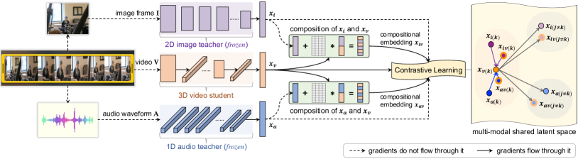
Figure 2: Given the image, video, audio embeddings encoded by individual networks (Section 3.1), compositional embeddings are learned to close the cross-modal semantic gap and capture the task-relevant semantics (Section 3.2), which, along with knowledge from the image and audio networks, are transferred to the video network by compositional contrastive learning in the shared latent space (Section 3.3).

Knowledge Distillation. A typical knowledge distillation paradigm follows a teacher-student learning strategy, where the knowledge learned by a large teacher network or an ensemble of networks is transferred to a lightweight student network [29, 7, 9, 23]. In general, supervision signals from the teacher regularise the student network during training, as represented by a cross-entropy loss on the soft targets [29], or a regression loss on the pre-softmax activation [7]. A line of works reformulate the supervision signals for more effective knowledge transfer, such as attention transfer [69], probabilistic transfer [45], relation transfer [44], and correlation transfer [48]. Another line of works distill knowledge in a cross-modal context [24, 6, 3, 34], such as learning sound representations [6], or optimising a depth estimation model [24] leveraging knowledge from a visual recognition model. In contrast to these recent works which assume different modalities share similar semantics or physical structures, we study a more challenging scenario using unconstrained videos with a possible cross-modal semantic gap.

Audio-Visual Learning. Audio has been used to assist visual learning or vice versa, e.g. to separate or localise sound in videos [40, 56, 5, 21], for audio recovery [70], lip reading [2], speech recognition [1], or audio-driven image synthesis [67, 31]. Several self-supervised methods have recently been explored for audio-visual learning [41, 42, 4, 47]. By training the audio and video networks jointly, these works leverage the semantic correspondence between audio and video for unsupervised learning on a large video dataset. To further scale audio-visual learning to unconstrained audio-video data with possible semantic mismatch, we propose to distill the audio-visual knowledge from pre-trained teacher networks to regularise the student network.

Contrastive Learning. The contrastive loss was initially proposed to learn invariant representations by mapping similar inputs to nearby points in a latent space [26]. Recently, a family of models popularised the idea of contrastive learning for self-supervised learning [30, 39, 18, 12, 11]. The aim is to maximise the mutual information between different views of the same instance [11, 18] or between the local and global features extracted from the same image [30]. To ensure its success, a memory bank is generally used to store a large amount of negative samples, while various data augmentation techniques are often used to produce many views of the same sample. Besides self-supervised learning, contrastive learning has recently been studied in other contexts, such as knowledge distillation [54] and image generation [43]. To our knowledge, we are the first to introduce contrastive learning to distill knowledge across heterogeneous modalities. Rather than using a vanilla contrastive loss (e.g. InfoNCE [39]), we formulate a multi-class noise contrastive estimation loss that utilises the class labels to efficiently associate positives and dissociate negatives across modalities.

Video Representations. To represent video information, early works often extract hand-crafted visual features by computing dense trajectories [63], SIFT-3D [51] and HOG-3D [33]. Recent advances in video representation learning have been achieved by learning spatiotemporal features with convolutional neural networks (CNNs) on large-scale video datasets, as represented by two-stream networks [52, 19], 3D-CNNs [57, 10, 27] and factorised 3D-CNNs [49, 58]. While these approaches are trained using annotated videos, some self-supervised methods learn video representations from a large collection of unlabelled videos by sorting video frames [68, 32], using temporal cycle consistency [16, 66] or video colorisation [62]. Recently, there has been a growing interest in learning multi-modal video representations with audio signals [65, 37] or video captions [20], which both aim to integrate the multi-modal cues into a single feature encoding to represent each video. Although our model also exploits the multi-modal semantics in videos, it uniquely leverages the privileged knowledge from multiple modalities without training multiple networks jointly, and processes only the video modality at test time for a higher efficiency.

3 Compositional Contrastive Learning (CCL)

Our goal is to distill audio-visual knowledge learnt from heterogeneous audio and image modalities for video representation learning, while the cross-modal content may be semantically unrelated. The image and audio embeddings are first extracted from pre-trained teacher networks (Figure 2, top and bottom), and then composed with the video embeddings (Figure 2, middle) to bridge the cross-modal semantic gap (Section 3.2). The unimodal audio and image embeddings, along with the compositional embeddings, are then jointly aligned with the video embeddings by compositional contrastive learning to distill audio-visual knowledge (Section 3.3). At test time, only the video student network is deployed for the video recognition or video retrieval tasks.

3.1 Unimodal Representations of Audio and Vision

Given a dataset of $N$ videos $\mathcal{D}=\{\textbf{V}_{i},y_{i}\}_{i=1}^{N}$ – each video belongs to one of $\mathcal{K}$ video categories and contains a set of images $\{{\textbf{I}_{ij}}\}_{j=1}^{M_{i}}$ with an audio recording $\textbf{A}_{i}$, we extract the unimodal embeddings via CNNs. As audio, image, and video data exhibit heterogeneous characteristics, different network architectures are adopted to model the temporal, spatial, or spatiotemporal information, as detailed next.

Audio Teacher Network. Although the audio and visual content in a video may not be semantically related, the audio knowledge encodes temporal context that offers rich privileged information [59]. Given the audio recording ${\bf A}_{i}$ of the video ${\bf V}_{i}$, the log-mel spectrogram is extracted and passed through a pre-trained 1D-CNN to obtain an audio embedding, formally referred to as $x_{a}=\theta_{\text{1D-CNN}}({\bf A}_{i})$, where $x_{a}$ is a $K_{a}$-dimensional audio teacher embedding, $\theta_{\text{1D-CNN}}$ is the audio teacher network parameterised by 1D convolutions to capture the temporal acoustic context.

Image Teacher Network. The image teacher network is a standard 2D-CNN to encode the spatial visual information. Given an image frame ${\bf I}_{ij}$ randomly sampled from the video ${\bf V}_{i}$, an image embedding is extracted using the 2D-CNN, referred to as $x_{i}=\theta_{\text{2D-CNN}}({\bf I}_{ij})$, where $x_{i}$ is a $K_{i}$-dimensional image teacher embedding, and $\theta_{\text{2D-CNN}}$ is the image teacher network. As each video clip contains a set of image frames, only one image frame is randomly selected at a time to represent the spatial visual content.

Video Student Network. To distill audio-visual knowledge from two teacher networks, a 3D-CNN network customised for video recognition is employed to learn the video representations from scratch, while mimicking the teacher networks (detailed in Section 3.3). The video network contains a stack of residual blocks with (2+1)D convolutions, which alternates between 2D spatial convolutions and 1D temporal convolutions to encode the spatiotemporal visual content. Given a $T{\times}H{\times}W{\times}3$ volume of an RGB video clip from video ${\bf V}_{i}$, a video embedding is parameterised by the 3D-CNN, formally referred to as $x_{v}=\theta_{\text{3D-CNN}}({\bf V}_{i})$, where $x_{v}$ is a $K_{v}$-dimensional video embedding, and $\theta_{\text{3D-CNN}}$ is the video student network trained by a cross-entropy loss to predict a probability distribution $P_{v}$ over $\mathcal{K}$ video classes:

$$\mathcal{L}_{ce}^{v}=\mathcal{L}_{ce}(x_{v},k)={-}\log\Big{(}P_{v}(k|{x}_{v};\theta_{cls})\Big{)},$$

where $k$ is the class label of ${\bf V}_{i}$, $\theta_{cls}$ is the video classifier.

3.2 Compositional Multi-Modal Representations

As aforementioned, the student and teacher embeddings may be semantically unaligned – an image frame may capture only partial visual cues not directly related to the video event, while the accompanied audio of an action video may be irrelevant music or speech. To bridge the possible semantic gap and domain gap across modalities, we propose to rectify the audio and image teacher embeddings by composing the teacher and student embeddings and constraining the compositional embeddings with our task objective to close the possible semantic gap. As the network architectures are nonuniform across different modalities, the cross-modal composition is derived at the penultimate layer.

Formally, the teacher embeddings $x_{a}$, $x_{i}$ are composed with the student embedding $x_{v}$ by learning a residual on top of the teacher embeddings. We rectify the teacher embeddings using the following composition function $\mathcal{F}(\cdot,\cdot)$, which learns a residual $f_{\theta}(\cdot,\cdot)$ that fuses two modalities by normalisation, concatenation and a linear projection:

$$\mathcal{F}_{av}(x_{a},x_{v}) =x_{av}=x_{a}+f_{{\theta_{av}}}(x_{a},x_{v}),$$ (1)

$$\mathcal{F}_{iv}(x_{i},x_{v}) =x_{iv}=x_{i}+f_{{\theta_{iv}}}(x_{i},x_{v}),$$

where $x_{av},x_{iv}$ are the compositional embeddings. This operation is related to prior works that compose multi-modal features [61, 14, 13], but ours aims at shifting the teacher embedding with a learnable residual. More importantly, to constrain the class assignment of the compositional embeddings, $\mathcal{F}(\cdot,\cdot)$ is optimised by the video classification loss (i.e. $\mathcal{L}_{\text{ce}}$), which ensures $x_{av},x_{iv}$ are assigned to the same video class label as $x_{v}$. The overall classification loss is:

$$\mathcal{L}_{cls}=\mathcal{L}_{ce}^{v}(x_{v},k)+\mathcal{L}_{ce}^{av}(x_{av},k)+\mathcal{L}_{ce}^{iv}(x_{iv},k),$$ (2)

where $\mathcal{L}_{ce}^{av},\mathcal{L}_{ce}^{iv}$ are imposed on the composition functions $\mathcal{F}_{av}(\cdot,\cdot),\mathcal{F}_{iv}(\cdot,\cdot)$. In the presence of a cross-modal semantic gap (e.g., the audio and video embeddings $x_{a}$, $x_{v}$ belong to different classes), the compositional embeddings are enforced to share the same class label $k$ as $x_{v}$. In other words, the compositional embeddings are learned to close the possible semantic gap and capture the task-relevant semantics to facilitate more informative knowledge transfer.

3.3 Distilling Audio-Visual Knowledge

Many prior unimodal methods distill knowledge merely in the prediction space by enforcing the student network to output similar predictions as the teacher network [29, 7, 9]. However, this strategy cannot be directly applied to multi-modal distillation, given the teacher networks are often pre-trained on heterogeneous task objectives to predict different classes. Thus, we propose to perform contrastive learning in the latent feature space, followed by contrasting the class distributions in the prediction space.

Given the unimodal embeddings and the compositional embeddings, we propose to distill the knowledge by pulling together the positive pairs while pushing away the negative pairs across modalities. The positive pairs could include the images, audios, and videos from the same video class $k$. Specifically, for a triplet of audio, video, and their compositional embeddings extracted from the video $\textbf{V}_{i}$, the contrastive loss can be formed in every pair among them to reinforce their correspondence in the shared embedding space. Formally, a contrastive loss $\mathcal{L}_{ct}$ (based on InfoNCE [39]) between a pair of audio and video embeddings $x_{v(i)},x_{a(i)}$ can be derived as below.

$$\mathcal{L}_{ct}{=}{-}\text{log}\frac{\text{exp}(\Phi(x_{v(i)},x_{a(i)})/\tau)}{\sum_{j=1}^{B}\text{exp}(\Phi(x_{v(j)},x_{a(j)}))/\tau)}{=}{-}\text{log}\ p_{av(i)},$$ (3)

where $\Phi$ is a cosine similarity scoring function, $\tau$ is the temperature, $p_{av(i)}$ is the probability of assigning the video embedding $x_{v(i)}$ to its paired audio embedding $x_{a(i)}$ against the whole mini-batch of audio embeddings $\{x_{a(j)}\}_{j=1}^{B}$.

Although the contrastive loss $\mathcal{L}_{ct}$ (Eq. (3)) has shown its success as an instance-level self-supervised signal [11, 12], it is not directly applicable in our context, given there may exist multiple positive video-audio pairs sampled from an identical video class $k$ per batch. Therefore, we formulate a multi-class noise contrastive estimation (NCE) loss that brings the class label $k$ into the loss formulation:

$$\mathcal{L}_{nce}(x_{v},x_{a}){=}{-}\frac{1}{B_{p}}\sum_{j=k}\text{log}\ p_{av(j)}{-}\frac{1}{B_{n}}\sum_{j{\neq}k}\text{log}(1{-}p_{av(j)}),$$ (4)

where $B_{p},B_{n}$ are the number of positive pairs (from class $k$) and negative pairs (not from class $k$) for the video embedding $x_{v}$ (labelled as $k$). When $B_{p}{=}B_{n}{=}1$, Eq. (4) is equivalent to the vanilla NCE [25]. Note that Eq. (3) considers each instance as a class; thus, using Eq. (3) would ignore the class-level discrimination and blindly treat some positives as false negatives. In contrast, our multi-class NCE (Eq. (4)) encourages the network to assign higher probabilities to the positives and lower probabilities to the negatives.

The same multi-class NCE loss can be imposed between the video embedding $x_{v}$ and the compositional embedding $x_{av}$ to collectively distill unimodal audio knowledge and multi-modal knowledge in a compositional manner:

$$\mathcal{L}_{a}(x_{v},x_{a},x_{av}){=}\lambda\mathcal{L}_{nce}(x_{v},x_{a})+(1-\lambda)\mathcal{L}_{nce}(x_{v},x_{av}),$$ (5)

where $\lambda$ is a hyperparameter to balance the two terms, $\mathcal{L}_{a}$ is the objective from the audio modality. Similarly, the above objective can be rewritten by utilising the image modality:

$$\mathcal{L}_{i}(x_{v},x_{i},x_{iv}){=}\lambda\mathcal{L}_{nce}(x_{v},x_{i})+(1-\lambda)\mathcal{L}_{nce}(x_{v},x_{iv}),$$ (6)

where $x_{i}$, $x_{iv}$ are the image embedding and the compositional embedding respectively. In essence, the loss function (Eq.(5) or Eq.(6)) serves as a similarity constraint to align embeddings in the multi-modal latent feature space. Since the compositional embeddings are constrained by the classifiers for video classification, a similarity constraint can also be imposed to further align the class distributions in the prediction space. Formally, given the predictive distributions from the video network $P_{v}$ and the composition functions $P_{av}$, $P_{iv}$, we introduce the Jensen–Shannon divergence (JSD) [36] to align $P_{v}$ with respect to $P_{av},P_{iv}$:

$$\mathcal{L}_{JSD}{=}JSD(P_{v}||P_{av})+JSD(P_{v}||P_{iv}),$$ (7)

where $JSD(P||Q)$ is a symmetric similarity measure between two distributions, i.e. $JSD(P||Q)=(KL(P||Q)+KL(Q||P))/2$. Minimising $\mathcal{L}_{JSD}$ contrasts the class semantics between $P_{v}$ and $P_{av},P_{iv}$ in the prediction space, which is orthogonal to feature-level contrastive learning.

Learning Objective. The final compositional contrastive learning objective (CCL) for distilling audio-visual knowledge in the video recognition task can be written as below.

$$\mathcal{L}_{CCL}=\mathcal{L}_{\text{distill}}+\lambda_{cls}\mathcal{L}_{cls},\text{with}\ \mathcal{L}_{\text{distill}}{=}\mathcal{L}_{i}{+}\mathcal{L}_{a}{+}\mathcal{L}_{JSD}$$ (8)

where the distillation objective $\mathcal{L}_{\text{distill}}$ optimises the model along with the classification objective $\mathcal{L}_{cls}$ (Eq. (2)). According to the availability of pre-trained networks from the image and audio modalities, $\mathcal{L}_{\text{distill}}$ can be flexibly rewritten as $\mathcal{L}_{i}{+}JSD(P_{v}||P_{iv})$ to distill visual-only knowledge, or $\mathcal{L}_{a}{+}JSD(P_{v}||P_{av})$ to distill audio-only knowledge. In our experiments (Section 4), we consider audio, visual, and audio-visual distillation to study the individual impact of each modality, as well as their combinative impact.

4 Experiments

Datasets. To establish a comprehensive multi-modal distillation benchmark, we use the following video datasets. (1) UCF51 [53] is a subset of UCF101 that contain audios in videos, including 6,845 videos from 51 action classes, such as baby crawling and apply lipstick. We use the public split 1 for evaluation. (2) ActivityNet [17] contains 14,950 videos, covering a wide range of 200 complex human daily activities, such as arm wrestling and having an ice cream. We use the default split (10,024 training vs 4,926 validation videos). (3) VGGSound [60] is a large-scale dataset of 309 audio-visual correspondent event classes from 199,196 videos, such as playing violin and thunder. We use 183,730 videos for training and the rest for testing. Note that except VGGSound, audio and video in the other two datasets are not always semantically correlated.

Implementation Details. We use R(2+1)D-18 [58] as the video student network. The audio and image teacher networks are the 1D-CNN14 [35] and 2D-ResNet34 [28], pre-trained on the AudioSet [22] and ImageNet [15]. The model weights of the teacher networks are kept frozen during training. The video network is trained by SGD with a learning rate of $0.001$, a weight decay of $0.0005$. The batch size is $16$ on UCF51, $64$ on ActivityNet, $256$ on VGGSound. The temperature $\tau$ is $0.1$, $0.5$ on the image and audio modality. The hyperparameters $\lambda,\lambda_{cls}$ are set to 0.5, 1. The dimension of the latent feature space is 512. As the feature dimensions of all networks are 512, we do not add projections upon the networks, but linear projections can be added to map all embeddings to the same dimensionality. The video clips are cropped to $112{\times}112$. Each clip contains 16 frames. We train the model without accessing the AudioSet or ImageNet. At test time, only the video network is used. More algorithmic details are given in the supplementary.

Tasks and Metrics. We evaluate the quality of video representations on video recognition and video retrieval tasks. The video network is trained for recognition, and tested for both recognition and retrieval. For recognition, top-1 accuracy (%) is reported to show the classification accuracy on the test set. For retrieval, R@K (recall@K, %) is reported, i.e. the top $k$ nearest neighbours (kNN) contain videos from the same class as the query videos. In kNN retrieval [8], videos in the test set are used as queries and videos in the training set are the retrieval targets. For each video, multiple clip-level features are extracted by applying a sliding window. The feature per video is computed by averaging all the clip-level features. A cosine distance metric is finally adopted to measure the pairwise similarity in kNN retrieval.

Method	UCF51			ActivityNet
	A	I	AI	A	I	AI
baseline	57.5	57.5	57.5	32.6	32.6	32.6
FitNet	48.4	67.4	62.4	21.3	45.8	34.6
PKT	53.2	58.2	62.0	33.4	35.4	35.1
COR	57.7	65.5	66.3	31.4	43.1	41.7
RKD	53.0	55.4	58.2	-	34.3	-
CRD	60.3	61.4	63.2	36.4	37.3	36.6
IFD	56.3	54.2	64.2	34.6	33.8	35.4
CMC	59.2	60.4	63.1	34.4	23.7	33.9
CCL	64.9	69.1	70.0	36.5	46.3	47.3

Table 1: Video recognition on UCF51 and ActivityNet. Metric: Top1 accuracy (%). Knowledge is transferred from A: audio; I: image; or AI: audio and visual modalities to improve the video recognition model (‘-’: the model is not converged).

4.1 Comparing with the State of the Art

Baseline and State-of-the-art Models. For a fair and comprehensive evaluation, we propose a multi-modal distillation benchmark, comparing our CCL to a simple baseline model without distillation and seven state-of-the-art distillation methods. We train each model similar to CCL, but replace the distillation objective based on their open-source implementation. In the following, we describe their distillation objectives in brief. FitNet [50] aligns the representations of the teacher and student by regression. PKT [45] models the feature distribution by a probabilistic model, and matches the distributions between the student and teacher by a divergence metric. CCKD [48] transfers the correlation among instances in the feature space from the teacher to the student by regression. RKD [44] transfers the distance-wise and angle-wise relations of features from the teacher to the student by penalising differences in relations. CRD [54] transfers knowledge by instance-level contrastive learning and uses a large memory bank to store negative samples. IFD [46] trains the student network to mimic the teacher’s information flow derived by a probabilistic model. CMC [55] is a cross-view learning method to align different views of the same instances by contrastive learning.

Remark. The above methods are proposed based on an assumption that the teacher and student are trained on the unimodal data or on the same task objective; while we uniquely consider to distill knowledge learned from heterogeneous multiple data modalities. Our model also differs in several aspects compared to other contrastive learning methods (CRD, CMC). First, we introduce learnable compositional embeddings to close the cross-modal semantic gap and capture task-relevant semantics. Second, rather than treating each instance as one class, our objective exploits the class labels to enhance discrimination of different classes. Third, we do not use a large memory bank, thus greatly lowering the computation cost to derive the contrastive loss.

Setup	UCF51									ActivityNet
	A			I			AI			A			I			AI
Metrics	R1	R5	R10	R1	R5	R10	R1	R5	R10	R1	R5	R10	R1	R5	R10	R1	R5	R10
baseline	57.3	65.3	68.9	57.3	65.3	68.9	57.3	65.3	68.9	29.0	46.5	54.9	29.0	46.5	54.9	29.0	46.5	54.9
FitNet	31.9	42.5	47.6	51.4	66.9	73.7	61.2	68.7	72.4	16.5	32.8	42.1	30.7	52.6	62.5	30.5	48.3	57.0
PKT	48.4	57.2	61.8	53.0	63.4	68.9	61.2	69.1	72.2	26.4	44.4	53.3	28.1	48.1	57.4	30.3	47.6	56.2
COR	51.7	58.6	61.4	56.1	66.9	73.7	52.8	65.1	72.6	27.3	45.7	54.9	33.2	55.2	64.6	30.2	51.7	61.7
RKD	46.6	56.8	61.8	51.2	59.7	65.3	55.8	63.7	66.9	-	-	-	27.1	47.1	56.1	-	-	-
CRD	59.5	65.8	68.0	59.1	66.5	69.1	61.0	66.9	70.1	31.6	50.4	58.9	32.3	50.7	58.6	33.1	49.8	58.2
IFD	53.8	60.8	65.6	48.0	58.6	65.3	64.3	71.1	74.2	28.9	47.1	56.1	25.3	44.4	54.4	30.0	47.6	56.1
CMC	57.9	64.5	67.7	60.1	63.5	65.0	62.9	69.0	71.7	30.0	49.1	57.6	25.2	44.2	53.6	30.9	48.2	55.9
CCL	62.9	68.0	70.4	66.8	73.5	76.5	67.6	72.3	74.7	30.6	49.1	57.3	38.1	58.8	67.4	39.5	59.3	67.4

Table 2: Video retrieval on UCF51 and ActivityNet. Metrics: R@K ($K=1,5,10$, %). Knowledge is transferred from A: audio; I: image; or AI: audio and visual modalities to improve the video recognition model ( ‘-’: the model is not converged).

Figure 3: The per-class top-1 video recognition accuracy for audio distillation on UCF51 comparing FitNet and CCL wrt the baseline. Light green and orange: FitNet and CCL outperform the baseline.

Video Recognition. In Table 1, we evaluate on three setups: audio distillation (A), visual distillation (I), and audio-visual distillation (AI) on the UCF51 and ActivityNet datasets. As shown in Table 1, distilling knowledge from all modalities, our CCL obtains the state-of-the-art consistently and improves over the prior methods. Specifically, when it comes to visual distillation with the image modality (I), we observe that FitNet is a strong competitor on both datasets. Similarly, when it comes to audio distillation (A), CRD obtains the prior state-of-the-art on both datasets. However, this observation does not hold on the other modality for both FitNet and CRD. On the other hand, our CCL makes better use of the knowledge learned from either the image or audio modality and thus outperforms all methods on both datasets, e.g. significantly boosting the baseline by 7.4% (64.9-57.5), 11.5% (69.1-57.6) on UCF51 (A) and (I).

On audio-visual distillation (AI), our CCL significantly outperforms the prior state-of-the-art on both datasets, obtaining an impressive result of 70.0% (vs 66.3% by COR) on UCF51 and 47.3% (vs 41.7% by COR) on ActivityNet. Although the prior state-of-the-art may perform well on audio or visual distillation (e.g. CRD, FitNet), this behaviour does not remain when it comes to multi-modal distillation, i.e. when using audio and visual modalities jointly. The new state-of-the-art obtained by our CCL in the setup of (AI) indicates its capability to distill the complementary knowledge from heterogeneous modalities in a robust manner.

Closer Look at Audio Distillation in Video Recognition. Although FitNet is a strong competitor in visual distillation, it does not perform as well in audio distillation. To better understand this discrepancy, we closely inspect the per-class top-1 video recognition accuracy on UCF51 using FitNet and our CCL in audio distillation. Our results in Figure 3 indicate that our model outperforms the baseline in most classes, while the performance of FitNet degrades in most classes (44 out of 51). As audio and video content are generally not semantically related on UCF51, when we look at individual classes, we find that FitNet mostly predicts incorrectly when the audio is not highly in line with the video content, e.g. in the class writing on board where FitNet fails, most videos show a person speaking while writing on board, and the audio is weakly related to the action. In the class table-tennis shot for which FitNet succeeds, many videos contain the related sound of the ball. More analyses are given in Section 4.2 and the supplementary.

As FitNet imposes a hard alignment by regression between the teacher and student, noisy side information from the audio teacher could bring a negative impact. Notably, our CCL is designed to close the cross-modal semantic gap and bring class labels into its loss formulation, thus showing robustness when distilling audio and (or) visual knowledge.

Video Retrieval. In Table 2, we evaluate all the methods in the video retrieval task on the three setups of audio (A), visual (I) and audio-visual (AI) distillation on the UCF51 and ActivityNet datasets. This is to test the discriminability of the video representations in a challenging scenario that requires more fine-grained discrimination between videos.

Our results in Table 2 indicate that while the other alternative distillation methods do not always exhibit better performance compared to the baseline, our model outperforms the baseline consistently with large margins. For instance, the best competitor (CRD) performs well overall, but its performance of audio or visual distillation on UCF51 is not always stronger than the baseline. Specifically, R@1 in audio distillation (A), our CCL obtains an impressive 62.9 (vs 59.5 by CRD) on UCF51 although it stays behind CRD on ActivityNet (30.6 by ours vs 31.6 by CRD). On the other hand, in the case of R@1 in visual distillation (I), our CCL outperforms CRD with large margins on both datasets (66.8 vs 59.1 on UCF51 and 38.1 vs 32.3 on ActivityNet).

Another observation is that, while many methods benefit from distilling audio-visual knowledge (AI), our model performs the best under this multi-modal setup. Our CCL significantly outperforms the state-of-the-art, giving a R@1 of 67.6 vs 64.3 by IFD on UCF51 and a R@1 of 39.5 vs 33.1 by CRD on ActivityNet. Using other metrics such as R@5 and R@10 on the smaller UCF51 dataset, the difference between the methods is smaller, e.g. on R@10 with audio-visual distillation, our CCL obtains 74.7 vs 74.2 by IFD. On the other hand, on the large-scale ActivityNet dataset, even on R@5 and R@10, our CCL significantly outperforms the state-of-the-art, e.g. on R@10 with audio-visual distillation, our CCL obtains 67.4 vs 61.7 by COR. These observations again suggest the robustness of our model for distilling knowledge from multiple modalities on different datasets, which are in line with the observations and trends on the video recognition task.

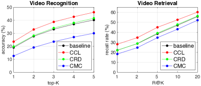
Figure 4: Results of CCL, CRD, CMC wrt the baseline on VGGSound. Left: recognition accuracy. Right: retrieval recall rate.

Experiments on the Large-scale VGGSound Dataset. So far, CCL has shown its success in audio-visual distillation in human action and activity video datasets. To further test our model’s generalisation on a challenging large-scale dataset of audio-visual events, we conduct experiments on the VGGSound dataset in the setup of audio-visual distillation (AI), where knowledge is jointly distilled from the audio and image modalities to improve the video modality. In addition to the baseline, we compare CCL to two strong competitors CRD, CMC that adopts contrastive learning. All methods are trained to predict the sound events in videos and tested for both video recognition and video retrieval tasks.

As Figure 4 shows, CCL (red curve) consistently outperforms the baseline (black curve) in both tasks, boosting the top-1 accuracy by 4.5% and the R@1 by 6.0% (exact numbers are given in the supplementary). While CRD (green curve) performs on par with the baseline, CMC performs lower than the baseline. Our results on VGGSound suggest the ability of CCL to generalise on a very large dataset, and demonstrate its capability to distill audio-visual knowledge for learning the video representations of sounds. Unlike the videos in UCF51 or ActivityNet, paired audio and video all share the same class semantics on VGGSound. This indicates the robustness of CCL in the different scenarios when the audio and video are either semantically correlated (VGGSound) or not always correlated (UCF51, ActivityNet).

4.2 Ablation Study and Qualitative Results

		UCF51
	Method	A	I	AI
	baseline	57.5	57.5	57.5
(a)	CCL w/o composition	63.2	65.8	66.9
(b)	CCL w $\mathcal{L}_{ct}$	60.4	68.4	67.8
	CCL w/o $\mathcal{L}_{nce}$	63.1	67.4	66.3
	CCL w/o $\mathcal{L}_{JSD}$	64.0	67.8	68.2
	CCL	64.9	69.1	70.0

Table 3: Ablation on (a) model component: CCL w/o composition; (b) loss formulation: CCL w $\mathcal{L}_{ct}$; CCL w/o $\mathcal{L}_{nce}$; CCL w/o $\mathcal{L}_{JSD}$, compared to the baseline and the CCL. Metric: Top1 (%).

To analyse our model formulation rationale, we conduct more studies on the UCF51 dataset in the following.

Ablation on Model Component. In the model formulation, our main idea is to learn a compositional embedding that closes the cross-modal gap and captures task-relevant semantics. Rather than transferring knowledge across modalities directly, our CCL distills the unimodal knowledge from the teacher networks and the multi-modal knowledge from the composition functions collectively. To verify the idea of composition, we compare CCL to an ablative baseline (CCL w/o composition). Table 3 (a) shows that removing the composition degrades the recognition performance by 1.7% (64.9-63.2), 3.3% (69.1-65.8), 3.1% (70.0-66.9) on the setup of (A), (I), (AI). This supports our motivation to compose representations across modalities. As the compositional embedding is learned to rectify the teacher embedding as constrained by the task objective, it brings the task-relevant semantics to improve cross-modal distillation.

Ablation on Loss Formulation. In the loss formulation, our goal is to associate positive pairs from the same class and disassociate negative ones. Our distillation objective brings class labels into contrastive learning, and performs alignment jointly in the feature and prediction space by the multi-class NCE ($\mathcal{L}_{nce}$) and the JSD loss ($\mathcal{L}_{JSD}$). To examine our objective empirically, we first compare our multi-class NCE $\mathcal{L}_{nce}$ (Eq. (4)) to an ablative baseline using the instance-level contrastive loss $\mathcal{L}_{ct}$ based on InfoNCE (Eq. (3)). Table 3 shows that CCL performs much better than the baseline “CCL w $\mathcal{L}_{ct}$”, improving the accuracy by 4.5% (64.9-60.4), 2.2% (70.0-67.8) on the setup of (A), (AI). This confirms the benefit of bringing class labels into contrastive learning. Next, we study the effect of similarity constraints in the feature and prediction space, we compare CCL to two ablative baselines: CCL w/o $\mathcal{L}_{nce}$, CCL w/o $\mathcal{L}_{JSD}$, which remove one constraint at a time. As Table 3 shows, CCL performs the best. Removing $\mathcal{L}_{nce}$ decreases the performance of CCL by 1.8% (64.9-63.1), 1.7% (69.1-67.4), 3.7% (70.0-66.3) in the setup of (A), (I), (AI); while removing $\mathcal{L}_{JSD}$ also leads to performance degradation. These results indicate that $\mathcal{L}_{nce}$, $\mathcal{L}_{JSD}$ are complementary and work synergistically to distill knowledge across modalities.

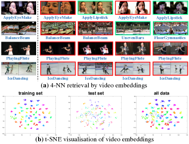
Figure 5: Qualitative results on UCF51. (a) Left: query videos; Right: 4-NN retrieved items. (b) Visualisation with t-SNE [38].

Qualitative Results. To understand the video representations qualitatively, we analyse CCL with qualitative results. For k-NN retrieval (Figure 5(a)), we observe that given the query videos, videos of the same or similar classes are retrieved, e.g. for the video “ice dancing”, the top retrieved videos are from the same class. For the video “apply eye makeup”, two videos are from the same class and the other two are from a similar action with subtle differences.

When visualising the video embeddings (Figure 5 (b)), we see that the embeddings of different classes (in different colours) are grouped into separated clusters; while the test set embeddings are lying on the manifolds similar to the training set. This means videos from training and test sets are grouped in a consistent way, where embeddings from the same class are associated with higher similarities. Our qualitative results overall show that CCL learns discriminative video representations from multi-modal distillation.

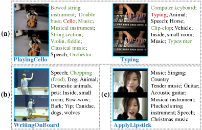
Figure 6: Audio-video correspondence: videos (labels in blue) from UCF51 and top-10 audio classes predicted by the audio network. Highly/weakly correlated audio events are in red/green. (a), (b), (c) denote video, audio are highly, weakly, or not correlated.

Qualitative Analysis on Cross-Modal Correspondence. To understand the cross-modal semantic gap, we provide visual examples of audio-video correspondence. As Figure 6 shows, based on the top-10 predicted audio classes, we can manually distinguish the audio-video correspondence as highly, weakly, or not correlated. In (a), the audio event “cello” is highly related to the video action. In (b), the audio is dominated by speech but contains the sound “chopping” weakly related to the sound made by “writing on board”. In (c), the audio is irrelevant “music”. These evidences are in line with our assumption of the cross-modal semantic gap in unconstrained videos. Similarly, an image frame may not capture the whole video action, leading to a possible semantic gap between the image and video modalities. Notably, our model tackles this issue by introducing the compositional embeddings for compositional contrastive learning. More analyses are given in the supplementary.

5 Discussion and Conclusion

We present a novel compositional contrastive learning (CCL) framework, a generic and effective approach to distill knowledge learned from heterogeneous data modalities for video representation learning. As there may exist a cross-modal semantic gap, we introduce the learnable compositional embeddings to close the gap and capture the task-related semantics. Our approach uniquely brings the unimodal knowledge (from teacher networks) and multi-modal knowledge (from composition functions) collectively to facilitate effective knowledge distillation. We compare our approach to a variety of state-of-the-art distillation methods, and demonstrate its performance advantages for both video recognition and video retrieval in different setups. Our empirical results also provide a realistic benchmark for future research in multi-modal distillation. As a future extension, our approach also opens up the possibility to bridge multiple modalities for multi-modal recognition and retrieval tasks.

Acknowledgements This work has been partially funded by the ERC (853489 - DEXIM) and by the DFG (2064/1 – Project number 390727645).

Algorithm A Compositional Contrastive Learning (Audio-Visual Distillation)

0:  Video dataset $\mathcal{D}=\{\textbf{V}_{i},y_{i}\}_{i=1}^{N}$, the corresponding image frames $\{{\textbf{I}_{ij}}\}_{j=1}^{M_{i}}$ and audio recording $\textbf{A}_{i}$ for each video.

0:  Trainable video student network $\theta_{\text{3D-CNN}}$. Pre-trained audio and image teacher networks $\theta_{\text{1D-CNN}},\theta_{\text{2D-CNN}}$.

1:  for $t=1$ to max_iter do

2:     $x_{a}\leftarrow\theta_{\text{1D-CNN}}({\bf A}_{i}),x_{i}\leftarrow\theta_{\text{2D-CNN}}({\bf I}_{ij}),x_{v}\leftarrow\theta_{\text{3D-CNN}}({\bf V}_{i})$ {obtain unimodal audio, image, video embeddings}

3:     $x_{av}\leftarrow\mathcal{F}_{av}(x_{a},x_{v})x_{iv}\leftarrow\mathcal{F}_{iv}(x_{i},x_{v})$ {derive compositional embeddings}

4:     $\mathcal{L}_{ce}^{v}\leftarrow\mathcal{L}_{ce}(x_{v},k),\mathcal{L}_{ce}^{av}\leftarrow\mathcal{L}_{ce}(x_{av},k),\mathcal{L}_{ce}^{iv}\leftarrow\mathcal{L}_{ce}(x_{iv},k)$ {compute video classification loss}

5:     $\mathcal{L}_{\text{audio}}\leftarrow\lambda\mathcal{L}_{nce}(x_{v},x_{a}){+}(1{-}\lambda)\mathcal{L}_{nce}(x_{v},x_{av}){+}JSD(P_{v}||P_{av})$ {compute audio distillation loss}

6:     $\mathcal{L}_{\text{image}}\leftarrow\lambda\mathcal{L}_{nce}(x_{v},x_{i}){+}(1{-}\lambda)\mathcal{L}_{nce}(x_{v},x_{iv}){+}JSD(P_{v}||P_{iv})$ {compute visual distillation loss}

7:     $\theta_{\text{3D-CNN}}^{t{+}1}\leftarrow\theta_{\text{3D-CNN}}^{t}{-}\eta\frac{\partial\mathcal{L}^{v}}{\partial\theta_{\text{3D-CNN}}}$, where $\mathcal{L}^{v}{=}\mathcal{L}_{ce}^{v}{+}\mathcal{L}_{\text{audio}}{+}\mathcal{L}_{\text{image}}$ {backprop on the video network}

8:     ${\theta_{av}^{t+1}}\leftarrow{\theta_{av}^{t}}{-}\eta\frac{\partial\mathcal{L}_{ce}^{av}}{\partial\theta_{av}},{\theta_{iv}^{t+1}}\leftarrow{\theta_{iv}^{t}}{-}\eta\frac{\partial\mathcal{L}_{ce}^{iv}}{\partial\theta_{iv}}$ {backprop on the composition functions}

9:  end for

F Additional Algorithm Details

Algorithm A gives an overview of our compositional contrastive learning (CCL) algorithm for audio-visual distillation. From an information-theoretic point of view, CCL distills audio-visual knowledge from the teacher networks by maximising the mutual information between the student network $\theta_{\text{3D-CNN}}$ and the teacher networks $\theta_{\text{1D-CNN}},\theta_{\text{2D-CNN}}$ and the composition functions $\mathcal{F}_{av},\mathcal{F}_{iv}$. While the multi-class contrastive loss $\mathcal{L}_{nce}$ contrasts the feature similarity, the Jensen–Shannon divergence $\mathcal{L}_{JSD}$ contrasts the prediction similarity, which together maximise the similarities between the cross-modal positive pairs from the same class. Importantly, class labels are introduced into both loss terms and the composition functions (Figure G), thus ensuring to transfer the task-relevant knowledge to the student network.

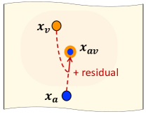
Figure G: Illustration of the compositional embedding $x_{av}$. The composition function uses residual learning to modify a teacher embedding $x_{a}$, which shifts $x_{a}$ towards the video embedding $x_{v}$, resulting in the compositional embedding $x_{av}$. Given the classification constraint $\mathcal{L}_{ce}$, $x_{av}$ is enforced to share to the same video class as $x_{v}$, thus closing the possible cross-modal semantic gap.

G Additional Analysis and Results

Analysis of Cross-Modal Correspondence. Here, we first manually analyse the audio-video correspondence on UCF51. For each video, we compute the top-10 predicted audio classes using the audio network. For each video class, we compute the top-10 associated audio classes based on how frequently they are predicted as the top-10 audio classes. We summarise the video classes and their top-10 associated audio classes in Tables G, H, I, where we manually classify the audio-video correspondence as highly, weakly and not correlated, as summarised in Table D.

audio-video correspondence	# video classes	proportion (%)
highly	15	29.4
weakly	15	29.4
not	21	41.2

Table D: Statistics of the audio-video correspondence on UCF51.

Figure H: Image-video correspondence: videos (tagged in blue) from UCF. The red/green boxes mean that the visual cues in the image frames are highly/weakly correlated to the video classes.

Moreover, we give some qualitative examples of the image-video correspondence (Figure H). As shown, the visual cues in image frames are generally highly or weakly related to the video content, e.g. the sea image is weakly correlated with the video class skijet due to occlusion.

Remark. Our analysis of the UCF51 dataset indicates the presence of a possible cross-modal semantic gap in multi-modal distillation. To empirically examine how CCL deal with this issue in practice, we evaluate CCL and its best competitor CRD using highly/weakly or not correlated audios for audio distillation. As Table E shows, on the 21 classes with not correlated audios, CRD performs on par with the baseline w/o distillation (+0.5% acc), while our CCL outperforms the baseline significantly (+3.1% acc). This suggests that our CCL can distill complementary information from audio even if it is uncorrelated with the video.

audio-video correspondence	baseline	CRD	CCL
weak/highly correlated (30 classes)	55.3	59.6	65.5
not correlated (21 classes)	61.0	61.5	64.1

Table E: Ablation study of audio distillation on UCF51.

Tabular Results on VGGSound. In Table F, we provide the tabular results of audio-visual distillation on the large-scale VGGSound dataset, which includes three contrastive learning methods (CRD, CMC, CCL) in comparison to the baseline for the video recognition and video retrieval tasks.

Task	Recognition		Retrieval
Metric	Top1	Top5	R1	R5	R10	R20
baseline	19.1	20.3	22.1	38.5	47.0	55.8
CRD	19.8	41.6	22.0	39.2	47.8	56.3
CMC	12.6	30.0	18.3	34.7	43.1	52.1
CCL	23.6	46.2	28.1	45.0	52.5	60.2

Table F: Audio-visual distillation on VGGSound.

2 Video Class	Top-10 Associated Audio Classes	Correlated
ApplyEyeMakeup	Speech; Inside, small room; Music; Female speech, woman speaking;	not
	Vehicle; Writing; Conversation; Narration, monologue; Animal; Rustle
ApplyLipstick	Speech; Music; Inside, small room; Vehicle; Animal; Female speech,	not
	woman speaking; Narration, monologue; Conversation; Musical instrument; Writing
Archery	Speech; Music; Vehicle; Arrow; Inside, small room; Outside,	highly
	rural or natural; Animal; Car; Door; Bird
BabyCrawling	Speech; Inside, small room; Music; Animal; Child speech, kid speaking; Babbling;	weakly
	Laughter; Domestic animals, pets; Vehicle; Crying, sobbing
BalanceBeam	Speech; Music; Vehicle; Outside, urban or manmade; Crowd; Inside,	weakly
	large room or hall; Inside, public space; Basketball bounce; Car; Animal
BandMarching	Music; Speech; Musical instrument; Drum; Percussion; Crowd; Orchestra;	highly
	Brass instrument; Vehicle; Wood block
BasketballDunk	Music; Speech; Vehicle; Basketball bounce; Outside, urban or manmade;	highly
	Crowd; Car; Hip hop music; Slam; Singing
BlowDryHair	Music; Speech; Vehicle; Inside, small room; Hair dryer; Vacuum cleaner;	highly
	Car; Mechanical fan; Animal; Train
BlowingCandles	Speech; Inside, small room; Music; Animal; Laughter; Chuckle, chortle;	not
	Snicker; Child speech, kid speaking; Inside, large room or hall; Domestic animals, pets
BodyWeightSquats	Speech; Music; Vehicle; Inside, small room; Male speech, man speaking;	not
	Narration, monologue; Animal; Musical instrument; Car; Conversation
Bowling	Speech; Music; Vehicle; Outside, urban or manmade; Train;	weakly
	Slam; Car; Animal; Inside, public space; Inside, large room or hall
BoxingPunchingBag	Speech; Music; Slam; Inside, large room or hall; Inside, small room;	weakly
	Thump, thud; Singing; Tap; Musical instrument; Vehicle
BoxingSpeedBag	Speech; Vehicle; Engine; Music; Car; Idling; Machine gun;	weakly
	Outside, urban or manmade; Engine starting; Motorcycle
BrushingTeeth	Speech; Inside, small room; Music; Animal; Toothbrush; Domestic animals,	highly
	pets; Scratch; Rub; Vehicle; Child speech, kid speaking
CliffDiving	Music; Speech; Vehicle; Musical instrument; Electronic music;	not
	Car; Rock music; Outside, urban or manmade; Guitar; Trance music
CricketBowling	Speech; Music; Vehicle; Outside, urban or manmade; Outside, rural or natural;	weakly
	Car; Animal; Basketball bounce; Slam; Inside, large room or hall
CricketShot	Speech; Music; Vehicle; Outside, urban or manmade; Arrow; Animal;	weakly
	Outside, rural or natural; Slam; Car; Thump, thud
2

Table G: Audio-video correspondence on the UCF51 classes. Video classes (1˜17), the top-10 associated audio classes, and the audio-video correlation: highly, weakly, or not correlated. Note: audio events highly/weakly correlated with the video are highlighted in red/green.

2 Video Class	Top-10 Associated Audio Classes	Correlated
CuttingInKitchen	Music; Speech; Inside, small room; Chopping (food); Dishes, pots, and pans;	highly
	Wood; Animal; Chop; Vehicle; Cutlery, silverware
FieldHockeyPenalty	Speech; Vehicle; Music; Outside, urban or manmade; Basketball bounce;	weakly
	Car; Animal; Crowd; Outside, rural or natural; Hubbub, speech noise, speech babble
FloorGymnastics	Music; Speech; Crowd; Cheering; Vehicle; Inside, large room or hall;	not
	Children shouting; Outside, urban or manmade; Singing; Whoop
FrisbeeCatch	Speech; Music; Vehicle; Outside, urban or manmade; Singing;	not
	Car; Pop music; Hubbub, speech noise, speech babble; Boat, Water vehicle; Crowd
FrontCrawl	Speech; Vehicle; Music; Water; Stream; Car; Boat, Water vehicle;	weakly
	Outside, urban or manmade; Splash, splatter; Outside, rural or natural
Haircut	Speech; Music; Inside, small room; Vehicle; Musical instrument; Animal; Inside, large room or hall;	not
	Electronic music; Outside, urban or manmade; Female speech, woman speaking
HammerThrow	Music; Speech; Vehicle; Outside, urban or manmade; Car; Male speech,	not
	man speaking; Animal; Musical instrument; Outside, rural or natural; Basketball bounce
Hammering	Music; Speech; Hammer; Whack, thwack; Chop; Tools;	highly
	Inside, small room; Musical instrument; Vehicle; Glass
HandstandPushups	Speech; Music; Vehicle; Animal; Inside, small room; Musical instrument;	not
	Singing; Domestic animals, pets; Car; Pink noise
HandstandWalking	Speech; Music; Vehicle; Animal; Outside, urban or manmade; Car;	not
	Inside, small room; Musical instrument; Singing; Domestic animals, pets
HeadMassage	Speech; Music; Vehicle; Outside, urban or manmade; Inside, small room;	not
	Musical instrument; Singing; Animal; Inside, large room or hall; Car
IceDancing	Music; Speech; Musical instrument; Vehicle; Orchestra; Singing;	not
	Theme music; Outside, urban or manmade; Television; Guitar
Knitting	Speech; Inside, small room; Music; Writing; Animal; Vehicle;	not
	Female speech, woman speaking; Conversation; Air conditioning; Narration, monologue
LongJump	Speech; Music; Outside, urban or manmade; Vehicle; Car; Basketball bounce;	weakly
	Inside, public space; Crowd; Hubbub, speech noise, speech babble; Run
MoppingFloor	Speech; Inside, small room; Music; Animal; Vehicle; Inside, large room or hall;	not
	Male speech, man speaking; Television; Narration, monologue; Domestic animals, pets
ParallelBars	Speech; Music; Crowd; Inside, large room or hall; Inside, public space;	weakly
	Outside, urban or manmade; Basketball bounce; Cheering; Slam; Vehicle
PlayingCello	Music; Musical instrument; Bowed string instrument; Cello; String section;	highly
	Violin, fiddle; Double bass; Classical music; Orchestra; Piano
2

Table H: Audio-video correspondence on the UCF51 classes. Video classes (18˜34), the top-10 associated audio classes, and the audio-video correlation: highly, weakly, or not correlated. Note: audio events highly/weakly correlated with the video are highlighted in red/green.

2 Video Class	Top-10 Associated Audio Classes	Correlated
PlayingDaf	Music; Drum; Musical instrument; Percussion; Drum kit;	highly
	Bass drum; Snare drum; Drum roll; Wood block; Rimshot
PlayingDhol	Music; Drum; Musical instrument; Percussion; Drum kit; Bass drum;	highly
	Wood block; Speech; Snare drum; Tabla
PlayingFlute	Musical instrument; Music; Flute; Wind instrument, woodwind instrument; Classical music;	highly
	Inside, small room; Bowed string instrument; Piano; Violin, fiddle; Speech
PlayingSitar	Music; Musical instrument; Sitar; Plucked string instrument;	highly
	Classical music; Carnatic music; Bowed string instrument; Speech; Tabla; Music of Asia
Rafting	Music; Speech; Vehicle; Singing; Musical instrument;	weakly
	Waves, surf; Ocean; Car; Waterfall; Guitar
ShavingBeard	Speech; Inside, small room; Music; Vehicle; Animal; Inside, large room or hall;	highly
	Electric shaver, electric razor; Outside, urban or manmade; Electric toothbrush; Buzz
Shotput	Speech; Music; Vehicle; Outside, urban or manmade; Animal; Car;	not
	Outside, rural or natural; Musical instrument; Hubbub, speech noise, speech babble; Singing
SkyDiving	Music; Musical instrument; Singing; Punk rock; Rock music; Heavy metal;	not
	Grunge; Progressive rock; Angry music; Rock and roll
SoccerPenalty	Speech; Outside, urban or manmade; Music; Vehicle; Basketball bounce;	weakly
	Crowd; Slam; Male speech, man speaking; Car; Inside, public space
StillRings	Speech; Music; Vehicle; Outside, urban or manmade; Car; Inside, public space;	not
	Basketball bounce; Crowd; Inside, large room or hall; Slam
SumoWrestling	Speech; Music; Crowd; Inside, large room or hall; Inside, public space;	weakly
	Outside, urban or manmade; Cheering; Chatter; Basketball bounce; Slam
Surfing	Music; Musical instrument; Vehicle; Speech; Rock music;	not
	Rock and roll; Punk rock; Guitar; Singing; Car
TableTennisShot	Speech; Music; Ping; Animal; Tap; Inside, small room;	highly
	Inside, large room or hall; Vehicle; Whack, thwack; Bouncing
Typing	Typing; Speech; Computer keyboard; Typewriter; Vehicle;	highly
	Inside, small room; Music; Animal; Engine; Sewing machine
UnevenBars	Music; Speech; Outside, urban or manmade; Vehicle; Crowd; Basketball bounce;	not
	Car; Cheering; Slam; Children shouting
WallPushups	Speech; Music; Inside, small room; Animal; Vehicle; Narration, monologue;	not
	Male speech, man speaking; Conversation; Female speech, woman speaking; Musical instrument
WritingOnBoard	Speech; Inside, small room; Music; Male speech, man speaking; Narration, monologue;	weakly
	Inside, large room or hall; Chopping (food); Writing; Chop; Conversation
2

Table I: Audio-video correspondence on the UCF51 classes. Video classes (35˜51), the top-10 associated audio classes, and the audio-video correlation: highly, weakly, or not correlated. Note: audio events highly/weakly correlated with the video are highlighted in red/green.

References

- [1] Triantafyllos Afouras, Joon Son Chung, Andrew Senior, Oriol Vinyals, and Andrew Zisserman. Deep audio-visual speech recognition. IEEE TPAMI, 2018.
- [2] Triantafyllos Afouras, Joon Son Chung, and Andrew Zisserman. Asr is all you need: Cross-modal distillation for lip reading. In ICASSP, 2020.
- [3] Samuel Albanie, Arsha Nagrani, Andrea Vedaldi, and Andrew Zisserman. Emotion recognition in speech using cross-modal transfer in the wild. In ACM MM, 2018.
- [4] Humam Alwassel, Dhruv Mahajan, Lorenzo Torresani, Bernard Ghanem, and Du Tran. Self-supervised learning by cross-modal audio-video clustering. In NeurIPS, 2020.
- [5] Relja Arandjelovic and Andrew Zisserman. Objects that sound. In ECCV, 2018.
- [6] Yusuf Aytar, Carl Vondrick, and Antonio Torralba. Soundnet: Learning sound representations from unlabeled video. In NeurIPS, 2016.
- [7] Jimmy Ba and Rich Caruana. Do deep nets really need to be deep? In NeurIPS, 2014.
- [8] Uta Buchler, Biagio Brattoli, and Bjorn Ommer. Improving spatiotemporal self-supervision by deep reinforcement learning. In ECCV, 2018.
- [9] Cristian Buciluǎ, Rich Caruana, and Alexandru Niculescu-Mizil. Model compression. In ACM SIGKDD, 2006.
- [10] Joao Carreira and Andrew Zisserman. Quo vadis, action recognition? a new model and the kinetics dataset. In CVPR, 2017.
- [11] Ting Chen, Simon Kornblith, Mohammad Norouzi, and Geoffrey Hinton. A simple framework for contrastive learning of visual representations. In ICML, 2020.
- [12] Xinlei Chen, Haoqi Fan, Ross Girshick, and Kaiming He. Improved baselines with momentum contrastive learning. arXiv preprint arXiv:2003.04297, 2020.
- [13] Yanbei Chen and Loris Bazzani. Learning joint visual semantic matching embeddings for language-guided retrieval. In ECCV, 2020.
- [14] Yanbei Chen, Shaogang Gong, and Loris Bazzani. Image search with text feedback by visiolinguistic attention learning. In CVPR, 2020.
- [15] Jia Deng, Wei Dong, Richard Socher, Li-Jia Li, Kai Li, and Li Fei-Fei. Imagenet: A large-scale hierarchical image database. In CVPR, 2009.
- [16] Debidatta Dwibedi, Yusuf Aytar, Jonathan Tompson, Pierre Sermanet, and Andrew Zisserman. Temporal cycle-consistency learning. In CVPR, 2019.
- [17] Bernard Ghanem Fabian Caba Heilbron, Victor Escorcia and Juan Carlos Niebles. Activitynet: A large-scale video benchmark for human activity understanding. In CVPR, 2015.
- [18] Marco Federici, Anjan Dutta, Patrick Forré, Nate Kushman, and Zeynep Akata. Learning robust representations via multi-view information bottleneck. In ICLR, 2020.
- [19] Christoph Feichtenhofer, Haoqi Fan, Jitendra Malik, and Kaiming He. Slowfast networks for video recognition. In ICCV, 2019.
- [20] Valentin Gabeur, Chen Sun, Karteek Alahari, and Cordelia Schmid. Multi-modal transformer for video retrieval. In ECCV, 2020.
- [21] Ruohan Gao and Kristen Grauman. Co-separating sounds of visual objects. In ICCV, 2019.
- [22] Jort F Gemmeke, Daniel PW Ellis, Dylan Freedman, Aren Jansen, Wade Lawrence, R Channing Moore, Manoj Plakal, and Marvin Ritter. Audio set: An ontology and human-labeled dataset for audio events. In ICASSP, 2017.
- [23] Rohit Girdhar, Du Tran, Lorenzo Torresani, and Deva Ramanan. Distinit: Learning video representations without a single labeled video. In ICCV, 2019.
- [24] Saurabh Gupta, Judy Hoffman, and Jitendra Malik. Cross modal distillation for supervision transfer. In CVPR, 2016.
- [25] Michael Gutmann and Aapo Hyvärinen. Noise-contrastive estimation: A new estimation principle for unnormalized statistical models. In AISTATS, 2010.
- [26] Raia Hadsell, Sumit Chopra, and Yann LeCun. Dimensionality reduction by learning an invariant mapping. In CVPR, 2006.
- [27] Kensho Hara, Hirokatsu Kataoka, and Yutaka Satoh. Can spatiotemporal 3d cnns retrace the history of 2d cnns and imagenet? In CVPR, 2018.
- [28] Kaiming He, Xiangyu Zhang, Shaoqing Ren, and Jian Sun. Deep residual learning for image recognition. In CVPR, 2016.
- [29] Geoffrey Hinton, Oriol Vinyals, and Jeff Dean. Distilling the knowledge in a neural network. arXiv preprint arXiv:1503.02531, 2015.
- [30] R Devon Hjelm, Alex Fedorov, Samuel Lavoie-Marchildon, Karan Grewal, Phil Bachman, Adam Trischler, and Yoshua Bengio. Learning deep representations by mutual information estimation and maximization. In ICLR, 2019.
- [31] Amir Jamaludin, Joon Son Chung, and Andrew Zisserman. You said that?: Synthesising talking faces from audio. IJCV, 2019.
- [32] Dahun Kim, Donghyeon Cho, and In So Kweon. Self-supervised video representation learning with space-time cubic puzzles. In AAAI, 2019.
- [33] Alexander Klaser, Marcin Marszałek, and Cordelia Schmid. A spatio-temporal descriptor based on 3d-gradients. In BMVC, 2008.
- [34] A. Sophia Koepke, Olivia Wiles, and Andrew Zisserman. Visual pitch estimation. In SMC, 2019.
- [35] Qiuqiang Kong, Yin Cao, Turab Iqbal, Yuxuan Wang, Wenwu Wang, and Mark D Plumbley. Panns: Large-scale pretrained audio neural networks for audio pattern recognition. arXiv preprint arXiv:1912.10211, 2019.
- [36] Jianhua Lin. Divergence measures based on the shannon entropy. IEEE Transactions on Information theory, 1991.
- [37] Yang Liu, Samuel Albanie, Arsha Nagrani, and Andrew Zisserman. Use what you have: Video retrieval using representations from collaborative experts. In BMVC, 2019.
- [38] Laurens van der Maaten and Geoffrey Hinton. Visualizing data using t-sne. JMLR, 2008.
- [39] Aaron van den Oord, Yazhe Li, and Oriol Vinyals. Representation learning with contrastive predictive coding. arXiv preprint arXiv:1807.03748, 2018.
- [40] Andrew Owens and Alexei A Efros. Audio-visual scene analysis with self-supervised multisensory features. In ECCV, 2018.
- [41] Andrew Owens, Jiajun Wu, Josh H McDermott, William T Freeman, and Antonio Torralba. Ambient sound provides supervision for visual learning. In ECCV, 2016.
- [42] Andrew Owens, Jiajun Wu, Josh H McDermott, William T Freeman, and Antonio Torralba. Learning sight from sound: Ambient sound provides supervision for visual learning. IJCV, 2018.
- [43] Taesung Park, Alexei A Efros, Richard Zhang, and Jun-Yan Zhu. Contrastive learning for unpaired image-to-image translation. In ECCV, 2020.
- [44] Wonpyo Park, Dongju Kim, Yan Lu, and Minsu Cho. Relational knowledge distillation. In CVPR, 2019.
- [45] Nikolaos Passalis and Anastasios Tefas. Learning deep representations with probabilistic knowledge transfer. In ECCV, 2018.
- [46] Nikolaos Passalis, Maria Tzelepi, and Anastasios Tefas. Heterogeneous knowledge distillation using information flow modeling. In CVPR, 2020.
- [47] Mandela Patrick, Yuki M Asano, Ruth Fong, João F Henriques, Geoffrey Zweig, and Andrea Vedaldi. Multi-modal self-supervision from generalized data transformations. In NeurIPS, 2020.
- [48] Baoyun Peng, Xiao Jin, Jiaheng Liu, Dongsheng Li, Yichao Wu, Yu Liu, Shunfeng Zhou, and Zhaoning Zhang. Correlation congruence for knowledge distillation. In ICCV, 2019.
- [49] Zhaofan Qiu, Ting Yao, and Tao Mei. Learning spatio-temporal representation with pseudo-3d residual networks. In CVPR, 2017.
- [50] Adriana Romero, Nicolas Ballas, Samira Ebrahimi Kahou, Antoine Chassang, Carlo Gatta, and Yoshua Bengio. Fitnets: Hints for thin deep nets. In ICLR, 2015.
- [51] Paul Scovanner, Saad Ali, and Mubarak Shah. A 3-dimensional sift descriptor and its application to action recognition. In ACM MM, 2007.
- [52] Karen Simonyan and Andrew Zisserman. Two-stream convolutional networks for action recognition in videos. In NeurIPS, 2014.
- [53] Khurram Soomro, Amir Roshan Zamir, and Mubarak Shah. Ucf101: A dataset of 101 human actions classes from videos in the wild. arXiv preprint arXiv:1212.0402, 2012.
- [54] Yonglong Tian, Dilip Krishnan, and Phillip Isola. Contrastive representation distillation. In ICLR, 2019.
- [55] Yonglong Tian, Dilip Krishnan, and Phillip Isola. Contrastive multiview coding. In ECCV, 2020.
- [56] Yapeng Tian, Jing Shi, Bochen Li, Zhiyao Duan, and Chenliang Xu. Audio-visual event localization in unconstrained videos. In ECCV, 2018.
- [57] Du Tran, Lubomir Bourdev, Rob Fergus, Lorenzo Torresani, and Manohar Paluri. Learning spatiotemporal features with 3d convolutional networks. In CVPR, 2015.
- [58] Du Tran, Heng Wang, Lorenzo Torresani, Jamie Ray, Yann LeCun, and Manohar Paluri. A closer look at spatiotemporal convolutions for action recognition. In CVPR, 2018.
- [59] Vladimir Vapnik and Rauf Izmailov. Learning using privileged information: similarity control and knowledge transfer. JMLR, 2015.
- [60] A Vedaldi, A Zisserman, H Chen, and W Xie. Vggsound: a large-scale audio-visual dataset. In ICASSP, 2020.
- [61] Nam Vo, Lu Jiang, Chen Sun, Kevin Murphy, Li-Jia Li, Li Fei-Fei, and James Hays. Composing text and image for image retrieval-an empirical odyssey. In CVPR, 2019.
- [62] Carl Vondrick, Hamed Pirsiavash, and Antonio Torralba. Anticipating visual representations from unlabeled video. In CVPR, 2016.
- [63] Heng Wang, Alexander Kläser, Cordelia Schmid, and Cheng-Lin Liu. Action recognition by dense trajectories. In CVPR, 2011.
- [64] Limin Wang, Yuanjun Xiong, Zhe Wang, Yu Qiao, Dahua Lin, Xiaoou Tang, and Luc Van Gool. Temporal segment networks: Towards good practices for deep action recognition. In ECCV, 2016.
- [65] Weiyao Wang, Du Tran, and Matt Feiszli. What makes training multi-modal classification networks hard? In CVPR, 2020.
- [66] Xiaolong Wang, Allan Jabri, and Alexei A Efros. Learning correspondence from the cycle-consistency of time. In CVPR, 2019.
- [67] Olivia Wiles, A. Sophia Koepke, and Andrew Zisserman. X2face: A network for controlling face generation using images, audio, and pose codes. In ECCV, 2018.
- [68] Dejing Xu, Jun Xiao, Zhou Zhao, Jian Shao, Di Xie, and Yueting Zhuang. Self-supervised spatiotemporal learning via video clip order prediction. In CVPR, 2019.
- [69] Sergey Zagoruyko and Nikos Komodakis. Paying more attention to attention: Improving the performance of convolutional neural networks via attention transfer. In ICLR, 2017.
- [70] Hang Zhou, Ziwei Liu, Xudong Xu, Ping Luo, and Xiaogang Wang. Vision-infused deep audio inpainting. In ICCV, 2019.