SoT: Delving Deeper into Classification Head for Transformer

Abstract

Transformer models are not only successful in natural language processing (NLP) but also demonstrate high potential in computer vision (CV). Despite great advance, most of works only focus on improvement of architectures but pay little attention to the classification head. For years transformer models base exclusively on classification token to construct the final classifier, without explicitly harnessing high-level word tokens. In this paper, we propose a novel transformer model called second-order transformer (SoT), exploiting simultaneously the classification token and word tokens for the classifier. Specifically, we empirically disclose that high-level word tokens contain rich information, which per se are very competent with the classifier and moreover, are complementary to the classification token. To effectively harness such rich information, we propose multi-headed global cross-covariance pooling with singular value power normalization, which shares similar philosophy and thus is compatible with the transformer block, better than commonly used pooling methods. Then, we study comprehensively how to explicitly combine word tokens with classification token for building the final classification head. For CV tasks, our SoT significantly improves state-of-the-art vision transformers on challenging benchmarks including ImageNet and ImageNet-A. For NLP tasks, through fine-tuning based on pretrained language transformers including GPT and BERT, our SoT greatly boosts the performance on widely used tasks such as CoLA and RTE. Code will be available at https://peihuali.org/SoT.

1. Introduction

Vision Transformer	DeiT-T [40]		T2T-7 [51]		T2T-14  [51]
	IN	IN-A	IN	IN-A	IN	IN-A
ClassT	72.2	7.3	71.7	6.1	81.5	23.9
WordT	77.95.7↑	15.58.2↑	73.72.0↑	7.81.7↑	82.10.6↑	26.6 2.7↑
ClassT+WordT	78.66.4↑	17.510.2↑	74.52.8↑	8.12.0↑	82.61.1↑	27.13.2↑
Language Transformer	GPT [33]		BERT-base [7]		BERT-large [7]
	CoLA	RTE	CoLA	RTE	CoLA	RTE
ClassT	54.3	63.2	54.8	67.2	60.6	73.7
WordT	56.11.8↑	65.01.8↑	56.41.6↑	69.01.8↑	61.40.8↑	74.40.7↑
ClassT+WordT	57.33.0↑	65.42.2↑	58.03.2↑	69.32.1↑	61.81.2↑	75.11.4↑

Table 1: Accuracies (%) of transformer models which use single classification token (ClassT), single word tokens (WordT) and their combination (ClassT+WordT). We showcase performance of vision transformers (i.e., DeiT and T2T) on ImageNet (IN) [6] and ImageNet-A (IN-A) [13], and that of language transformers (i.e., GPT and BERT) on CoLA [46] and RTE [2]. The results indicate word tokens per se are very competent with classifier and moreover, are complementary to the classification token. See Sec. 4 for details and for diverse results.

In the past years transformer models have been very successful in the field of natural language processing (NLP) [41, 7, 33]. The transformer architecture, solely based on attention mechanisms, can naturally model long-range dependency of tokens and learn contextual knowledge. In contrast, the convolutional neural networks (CNNs) [49, 22] lack such capability as the convolutions are fundamentally local operations. The success of transformer models has attracted great interests of computer vision (CV) researchers [45, 1, 11, 21]. Recently, a vision transformer model called ViT [8] is proposed entirely based on a stack of transformer blocks, which has matched or outperformed state-of-the-art CNNs when pre-trained on ultra large-scale datasets of ImageNet-21K [6] or JFT-300M [38]. Thereafter, a number of pure transformer models, e.g.,  [51, 52, 44], have been proposed to improve the architecture of transformers, reporting impressive performance gains when trained from scratch on ImageNet with 1K classes [6].

Despite great advance, for years pure transformer models invariably build final classifier exclusively based on classification token, without explicitly harnessing high-level word tokens. Although the classification token interacts with all word tokens  through the attention mechanisms across the network backbone, we conjecture the high-level word tokens by themselves contain rich information that the classification token fails to accommodate. Therefore, exploiting only the classification token but excluding the word tokens from the classifier limits transformer models. Actually, we empirically find that rich information inherent in word tokens per se is very competent with classifier and moreover, is complementary to the classification token.

As show in Tab. 1, the experimental results on both CV and NLP tasks show that classification head solely based on word tokens (i.e., WordT) is often better than that based on single classification token (i.e., ClassT), and combination of WordT and ClassT further boosts the classification accuracy. Based on the empirical observations above, we rethink classification head for transformer, and propose a novel transformer model, namely second-order transformer (SoT), to exploit simultaneously classification token and word tokens for the final classifier. To this end, there exist two key issues to be tackled: (1) how to effectively aggregate the word tokens to fully explore their rich information; (2) how to explicitly combine word tokens with classification token for building the final classification head.

For effective token aggregation, we propose a multi-headed global cross-covariance pooling (MGCrP) method, which learns a group of second-order, cross-covariance representations. Previous works [24, 42] have shown that structured normalization plays an important role for the second-order representations. Unfortunately, existing structured normalization methods are not applicable to our MGCrP as it produces asymmetric matrices. Therefore, we present a singular value power normalization (svPN) method in light of the overall statistical analysis of data; moreover, an approximate, fast svPN algorithm is developed for guaranteeing efficiency. MGCrP shares similar philosophy and so is more consistent with the transformer block, clearly better than global average pooling (GAP) [25, 39, 12] and global covariance pooling (GCP) [26, 42] widely used in CNNs.

To build the classification head by combining word tokens with classification token, we propose three early fusion schemes, which combine the two kinds of token representations through operations such as concatenation and sum, along with one late fusion scheme which integrates individual classification scores. These schemes are illustrated in Fig. 2 and their comparisons are given in Tab. 3(b); among them, the sum scheme performs best. Note that the proposed classification head is architecture-agnostic, which can be seamlessly integrated into a wide variety of vision transformers and language transformers. To verify the effectiveness of our SoT, we conduct experiments on both CV and NLP tasks.

Our contributions are summarized as follows.

• We dig into the transformer’s classification head, finding that word tokens per se are very competent with classifier and moreover, is complementary to classification token. Based on this, we propose a second-order transformer (SoT) model. As far as we know, our SoT makes the first attempt to exploit simultaneously classification token and word tokens for classification, which can span and benefit both CV and NLP tasks.

• We propose multi-headed global cross-covariance pooling with structured normalization for mining word tokens, while systemically studying several schemes to combine word tokens with classification token. As a result, we achieve a novel classification head, which is very effective and suitable for a variety of transformer architectures.

• We perform thorough ablation study to validate our SoT. Extensive experiments show our SoT can significantly improve vision transformers on challenging ImageNet and ImageNet-A. Meanwhile, our SoT is very helpful to language transformers such as BERT and GPT, performing better than its conventional counterpart on General Language Understating tasks.

2. Related Works

Transformer architectures Solely based on attention mechanisms without any recurrence and convolutions, the transformer models [41] can naturally model long-range dependencies and global context, outperforming LSTM [15] and CNN [9] on NLP tasks. The transformer models pre-trained on large-scale unlabeled corpus (e.g., GPT [33, 34] and BERT [7]) are able to learn powerful language representations, and, after fine-tuning, achieve state-of-the-art results for a wide range of downstream language tasks [33, 34, 7, 29]. For CV tasks, Dosovitskiy et al. [8] present a pure transformer architecture (i.e., ViT) which reports very promising performance when pre-trained on ultra large-scale datasets. The works that follow greatly improve over ViT. DeiT [40] proposes an extra distillation token to transfer knowledge from teacher models. T2T-ViT [51] and PS-ViT [52] focus on better tokenization of vision patches. Swin Transformer [30] and PVT-T [44] introduces hierarchical structure into the transformer. Conformer [32] is a dual architecture which combines CNN with transformer. The pure transformer architectures, either in NLP or CV field, only use the classification token for the classifier, limiting the performance of models. As such, we propose a novel classification head, which exploits simultaneously the classification token and word tokens.

Second-order pooling GCP, also known as bilinear pooling, often produces symmetric positive definite (SPD) matrices as global representations [17, 28]. It can capture second-order relations, performing much better than GAP which only estimates first-order statistics [26, 42]. Research has shown that normalization techniques are very helpful to the second-order representations [28, 50, 24, 17]. Element-wise normalization improves GCP but fails to consider holistic structure of data [28]. The structured normalization such as matrix power normalization (MPN) [24, 42, 27] exploits the overall statistical structure and geometric structure of covariance matrices, and has greatly benefited GCP. As MPN depends on GPU-unfriendly eigen-decomposition, iSQRT [23] proposes a fast method for computing matrix square root, suitable for parallel implementation on GPU. A recent study [43] has shown that GCP with MPN improves Lipschitzness of the loss function, leading to fast convergence and robustness to distorted images. Different from GCP, we propose multi-headed global cross-covariance pooling, which shares similar philosophy and is consistent with transformers; furthermore, we propose a new structured method to normalize cross-covariance matrices.

3. Second-order Transformer (SoT)

In this section, we first describe the SoT network, followed by the proposed multi-headed global cross-covariance pooling method. Finally, we introduce the normalization method for cross-covariance matrices.

3.1. SoT Network

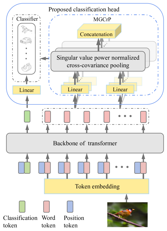
We illustrate our SoT network in Fig. 1. Similar to [52], we develop a small, hierarchical module for token embedding, which, based on off-the-shelf convolutions, gradually reduces spatial size of feature maps. In designing the token embedding module, we evaluate varying type of convolution blocks including ResNet block [12], Inception block [39], DenseNet block [16] and Non-local block [45]. This token embedding method has capability to model local image properties, which ViT [8] lacks due to its naive embedding method.

The features produced by the token embedding module are reshaped to a sequence of vectors as word tokens. As in [8], we prepend a learnable classification token to the word token sequence, and then position embeddings are added. The modified token sequence is then fed to the backbone network, which consists of a stack of standard transformer blocks, each containing a multi-head self-attention and a multi-layer perception.

For classification head, unlike the conventional transformers, we explicitly combine the word tokens with the classification token. We investigate different fusion methods to combine two kinds of tokens, finding the sum scheme performs best which, therefore, is adopted in our SoT. We design a family of transformers of varying depths, including a 12-layer SoT-Tiny, a 14-layer SoT-Small and a 24-layer SoT-Base; in addition, we design a 7-layer SoT for the sake of ablation study. The details on these models as well as on the token embedding module are provided in the supplement A.

Figure 1: Diagram of our SoT network. Given an input image, the token embedding module produces a sequence of word tokens, which is then prepended by a classification token. After added by position tokens, the sequence of tokens is subject to the backbone consisting of a stack of standard transformer blocks. Finally, the classification token and the word tokens output from the backbone are fed to the proposed classification head.

3.2. Proposed Classification Head

The conventional pure transformer models only use classification token for the final classifier. As high-level word tokens contain rich information, neglect of them leads to information loss. So we propose to combine the word tokens with the classification token for the final classifier.

We introduce three early fusion schemes (i.e., $\mathrm{sum}$, $\mathrm{concat}$ and $\mathrm{aggr\_all}$) and a late fusion scheme (i.e., $\mathrm{late}$). Fig. 2 illustrates these schemes, where a $\mathrm{Linear}$ transformation is equivalent to (and thus denoted by) a fully-connected (FC) layer. For the $\mathrm{sum}$ scheme, the classification token and aggregated word tokens are separately connected to a FC layer and are then summed, before fed to the softmax classifier. In the $\mathrm{concat}$ scheme, the representations of classification token and the aggregated word tokens are concatenated, followed by a FC layer and then a softmax classifier. For the $\mathrm{aggr\_all}$ scheme, we directly aggregate all tokens including both the classification token and the word tokens, and then connect the resulting representation to a FC layer succeeded by a softmax classifier. In the late fusion scheme, the classification token and the word tokens are independently attached to a FC layer and a softmax classifier, and finally the two classification scores are added.

(a) Sum

(b) Concat

(c) Aggr_all

(d) Late

Figure 2: Fusion schemes designed for our classification head.

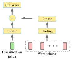
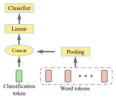
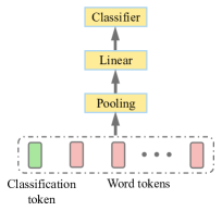
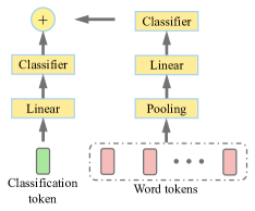
Let $\{\mathbf{z}_{i}\in\mathbb{R}^{p},i=0,1,\ldots,q\}$ denote the features of all tokens, where $\mathbf{z}_{0}$ indicates the classification token while the remaining ones indicate word tokens. We concatenate the features of word tokens to form a matrix $\mathbf{Z}=[\mathbf{z}_{1},\mathbf{z}_{2},\cdots,\mathbf{z}_{q}]\in\mathbb{R}^{p\times q}$. The four fusion schemes can be formulated as

$$\mathrm{sum}:\;\; \mathrm{softmax}\big{(}\mathrm{FC}(\mathbf{z}_{0})+\mathrm{FC}(\mathrm{pool}(\mathbf{Z})\big{)}$$ (1)

$$\mathrm{concat}:\;\; \mathrm{softmax}\left(\mathrm{FC}\left(\big{[}\mathbf{z}_{0},\mathrm{pool}(\mathbf{Z})\big{]}\right)\right)$$

$$\mathrm{aggr\_all}:\;\; \mathrm{softmax}\big{(}\mathrm{FC}(\mathrm{pool}([\mathbf{z}_{0},\mathbf{Z}])\big{)}$$

$$\mathrm{late}:\;\; \mathrm{softmax}\big{(}\mathrm{FC}(\mathbf{z}_{0})\big{)}+\mathrm{softmax}\big{(}\mathrm{FC}(\mathrm{pool}(\mathbf{Z}))\big{)}$$

Here $\mathrm{pool}(\cdot)$ denotes a pooling function. The commonly used pooling functions are global average pooling (GAP) and Global covariance pooling (GCP), which, however, are developed for CNN architecture and may be sub-optimal for the transformer. As described in [41, Sec. 3.2.2], the multi-head structure in the transformer block facilitates modeling information from different representation space. Inspired by this, we propose multi-headed global cross-covariance pooling (MGCrP) with structured normalization, as illustrated in Fig. 1 (top-right).

Pooling method	Formula	Matrix property	Structured Norm	Multi- head
GAP	$\frac{1}{q}\mathbf{Z}\mathbf{1}$	Vector	N/A	✗
GCP	$\mathrm{MPN}\left(\frac{1}{q}\mathbf{Z}\mathbf{Z}^{T}\right)$	SPD	MPN	✗
MGCrP (ours)	$\left[\mathrm{svPN}\left(\frac{1}{q}\mathbf{W}_{1}\mathbf{Z}\mathbf{Z}^{T}\mathbf{R}_{1}^{T}\right),\ldots,\right.$ $\left.\mathrm{svPN}\left(\frac{1}{q}\mathbf{W}_{h}\mathbf{Z}\mathbf{Z}^{T}\mathbf{R}_{h}^{T}\right)\right]\vspace{2pt}$	Asym	$\mathrm{svPN}$	✓

Table 2: Differences of our MGCrP from the classical pooling methods. GAP produces first-order, vectorial representations; GCP produces symmetric positive definite (SPD) matrices to which matrix power normalization (MPN) is applicable; MGCrP yields asymmetric matrices, normalized by the proposed singular value power normalization ($\mathrm{svPN}$).

In the following, we first introduce cross-covariance pooling with single head. Given an input matrix $\mathbf{Z}$, we perform two separate linear transformations, obtaining $\mathbf{X}=\mathbf{W}\mathbf{Z}$ and $\mathbf{Y=RZ}$, where $\mathbf{W}\in\mathbb{R}^{m\times p}$ and $\mathbf{R}\in\mathbb{R}^{n\times p}$ are learnable weight matrices. Then we compute cross-covariance matrix $\mathbf{Q}=\frac{1}{q}\mathbf{X}\mathbf{Y}^{T}$. Previous works have shown that structured normalization plays an important role for GCP. However, as $\mathbf{Q}$ is asymmetric (square or non-square), existing normalization method for SPD matrices [42] is not applicable. Thus we propose a new structured normalization method, called singular value power normalization (i.e., $\mathrm{svPN}$), details of which are deferred to next section. Now we can define our global cross-covariance pooling:

$$\mathrm{GCrP}(\mathbf{Z})=\mathrm{svPN}\Big{(}\frac{1}{q}\mathbf{W}\mathbf{Z}\mathbf{Z}^{T}\mathbf{R}^{T}\Big{)}$$ (2)

We continue to equip our cross-covariance pooling with multi-head structure:

$$\mathrm{MGCrP}(\mathbf{Z}) =\Big{[}\mathrm{GCrP}_{1}(\mathbf{Z}),\cdots,\mathrm{GCrP}_{h}(\mathbf{Z})\Big{]}$$

$$\mathrm{where}\ \mathrm{GCrP}_{i}(\mathbf{Z}) =\mathrm{svPN}\Big{(}\frac{1}{q}\mathbf{W}_{i}\mathbf{Z}\mathbf{Z}^{T}\mathbf{R}_{i}^{T}\Big{)}$$ (3)

Here $[\cdot]$ denotes concatenation operation; $\mathrm{GCrP}_{i}(\mathbf{Z})$ denotes the cross-covariance matrix of the $i$-th head, and $\mathbf{W}_{i}$ and $\mathbf{R}_{i}$ are two learnable linear projections.

Differences among GAP, GCP and MGCrP are summarized in Tab. 2, where $\mathbf{1}$ in the formula of GAP denotes a $q$-dimensional vector each component of which is 1, and we use state-of-the-art MPN [24] for GCP. Performance comparison among them is presented in Tab. 3(b). Ablation analysis on MGCrP is given in Sec. 4.2.2.

3.3. Normalization of Cross-covariance Matrix

We propose singular value power normalization (svPN) for cross-covariance matrices. As svPN is computationally expensive, we further develop a fast approximate algorithm.

3.3.1    Singular Value Power Normalization

Our method is motivated by MPN [42], an effective method for normalizing any covariance matrix $\mathbf{P}=\mathbf{Z}\mathbf{Z}^{T}$  that is SPD. This normalization consists in computation of power of eigenvalues aligned with eigenvectors of $\mathbf{P}$. In terms of principal component analysis [3, Chap. 12], the eigenvalues of $\mathbf{P}$ in decreasing order amounts to from maximum to minimum variances of $\mathbf{Z}$ , while the corresponding eigenvectors of $\mathbf{P}$ characterize the principal components. Therefore, MPN can be interpreted as shrinking these variances aligned with the principal components.

Let us consider $\mathbf{u}^{T}\mathbf{X}\mathbf{Y}^{T}\mathbf{v}$ where $\mathbf{u}\in\mathbb{R}^{m},\mathbf{v}\in\mathbb{R}^{n}$, which indicates the cross-covariance between projections of $\mathbf{X}$ on $\mathbf{u}$ and those of $\mathbf{Y}$ on $\mathbf{v}$. For simplification, we denote $\mathbf{Q}=\mathbf{X}\mathbf{Y}^{T}$. Actually, we have a proposition about such cross-covariances.

Proposition 1.

Given $\mathbf{u}_{i}$ and $\mathbf{v}_{i}$ where $i=1,\ldots,k-1$, let us consider the objective

$$\max_{\|\mathbf{u}\|=\|\mathbf{v}\|=1}\; \mathbf{u}^{T}\mathbf{X}\mathbf{Y}^{T}\mathbf{v}$$ (4)

$$\mathrm{s.t.}\;\; \mathbf{u}_{i}^{T}\mathbf{u}=0,\;\mathbf{v}_{i}^{T}\mathbf{v}=0,\;i<k.$$

By inductively optimizing (4) for $k=1,\ldots,\min(m,n)$, we can obtain, in decreasing order, the $k$-th largest cross-covariance $\mathbf{u}_{k}^{T}\mathbf{X}\mathbf{Y}^{T}\mathbf{v}_{k}$, which is equal to the $k$-th singular value $\lambda_{k}$ of $\mathbf{Q}$ while $\mathbf{u}_{k}$ and $\mathbf{v}_{k}$ are the corresponding left and right singular vectors, respectively.

In light of this proposition, we can define our normalization by shrinking the cross-covariances between $\mathbf{X}$ and $\mathbf{Y}$ aligned with the left and right singular vectors of $\mathbf{Q}$:

$$\mathrm{svPN}(\mathbf{Q})=\sum_{i=1}^{\min(m,n)}\lambda_{i}^{\alpha}\mathbf{u}_{i}\mathbf{v}_{i}^{T},$$ (5)

where $0\!\!<\!\!\alpha\!\!<\!\!1$. Our $\mathrm{svPN}$ can be performed accurately via SVD, which, however, is computationally expensive, as the SVD algorithm is GPU-unfriendly [23]. We give a proof of Proposition 1 and the backpropagation of svPN via SVD in the supplement B and C, respectively.

3.3.2    Fast Approximate Normalization Algorithm

Based on low-rank assumption widely used in machine learning [10], we can efficiently implement approximate normalization by only estimating few largest singular values. We use an iterative method to consecutively estimate the singular values. Given an initial vector $\mathbf{v}^{(0)}$, the iterative procedure takes the following form [37]:

$$\mathbf{u}^{(j+1)}=\dfrac{\mathbf{Q}\mathbf{v}^{(j)}}{\|\mathbf{Q}\mathbf{v}^{(j)}\|},\;\mathbf{v}^{(j+1)}=\dfrac{\mathbf{Q}^{T}\mathbf{u}^{(j+1)}}{\|\mathbf{Q}^{T}\mathbf{u}^{(j+1)}\|}$$ (6)

where the superscript $j$ denotes the $j$-th iteration. After a few iterations, we obtain approximately the largest singular value $\hat{\lambda}_{1}=\|\mathbf{Q}^{T}\mathbf{u}^{(j+1)}\|$ and the corresponding left singular vector $\hat{\mathbf{u}}_{1}=\mathbf{u}^{(j+1)}$ and right one $\hat{\mathbf{v}}_{1}=\mathbf{v}^{(j+1)}$.

Suppose we have the $k$-th ($k\geq 1$) largest singular value, we deflate matrix $\mathbf{Q}$ to obtain

$$\mathbf{Q}^{\prime}=\mathbf{Q}-\sum_{i=1}^{k}\hat{\lambda}_{i}\hat{\mathbf{u}}_{i}\hat{\mathbf{v}}_{i}^{T}$$ (7)

For $\mathbf{Q}^{\prime}$, we can perform iteration with Eq. (6) to achieve approximately the $(k+1)$-th largest singular value $\hat{\lambda}_{k+1}$ and the corresponding singular vectors $\hat{\mathbf{u}}_{k+1}$ and $\hat{\mathbf{v}}_{k+1}$. The deflation (7) and the iteration (6) can be repeated. Given $r$ largest singular values, we define the approximate normalization as

$$\widehat{\mathrm{sv}}\mathrm{PN}(\mathbf{Q})\!=\!\sum_{i=1}^{r-1}\hat{\lambda}_{i}^{\alpha}\hat{\mathbf{u}}_{i}\hat{\mathbf{v}}_{i}^{T}\!+\!\dfrac{1}{\hat{\lambda}_{r}^{1-\alpha}}\big{(}\mathbf{Q}\!-\!\sum_{i=1}^{r-1}\hat{\lambda}_{i}\hat{\mathbf{u}}_{i}\hat{\mathbf{v}}_{i}^{T}\big{)}$$ (8)

It shrinks the 1st to the $(r-1)$-th singular values aligned with the corresponding singular vectors, while shrinking the remaining ones with the $r$-th largest singular value. Note that $\widehat{\mathrm{sv}}\mathrm{PN}(\mathbf{Q})$ reduces to $\mathbf{Q}/\hat{\lambda}_{1}^{1-\alpha}$ if we only use the largest singular value.

4. Experiments

We first introduce experimental setting in Sec. 4.1. Then we evaluate the proposed methods for computer vision (CV) tasks and natural language processing (NLP) tasks in Sec. 4.2 and Sec. 4.3, respectively. We train models with 8 NVIDIA 2080Ti GPUs based on PyTorch framework. Our code will be open-sourced after acceptance.

4.1. Experimental Setting

Here we briefly describe the benchmarks and training strategy for both CV and NLP tasks. Details on benchmark statistics, task description and hyper-parameters setting are given in the supplement D.

Datasets For CV tasks, we evaluate on ILSVRC ImageNet benchmark [36, 6], which has 1.28M images for training and 50K images for test. Furthermore, we adopt a more challenging dataset (i.e., ImageNet-A [13]) for evaluation, which consists of real-world adversarial images, involving heterogeneous and varied distribution shift.

For NLP tasks, following the common practice [33, 7], we fine-tune the transformer models pre-trained in an unsupervised manner on large-scale corpus on four downstream tasks, i.e., Corpus of Linguistic Acceptability (CoLA) [46], Recognizing Textural Entailment (RTE) [2], Multi-Genre Natural Language Inference (MNLI) [47] and Stanford Question Answering (QNLI) [35].

Training strategy In image classification, we train our SoT models on ImageNet from scratch. Besides scale, color and flip augmentations [20, 12], following [51], we also adopt mixup [54], randAugment [5], cutmix [53], and label smoothing [39]. We use AdamW [31] algorithm with warmup for network optimization and cosine annealing schedule for learning rate. Detailed training strategies about optimizers, hyper-parameters, etc., are given in the supplement D. Also, we present in detail the hyper-parameter setting on natural language processing tasks in the supplement D.

4.2. Image Classification for CV Tasks

To make our extensive evaluations computationally feasible on ImageNet, in Sec. 4.2.1 and Sec. 4.2.2, we use the 7-layer SoT model; besides, we re-scale the images such that their short sizes are 128 and 112$\times$112 patches are cropped as network inputs. In Sec. 4.2.3, we compare with state-of-the-art methods using standard protocol on ImageNet.

4.2.1.   How Does Our Classification Head Perform?

We first establish a strong baseline model that only uses the classification token. Based on this strong baseline, we compare different fusion schemes and pooling methods.

Baseline based on conventional classification head Several works [51, 52] improve the simple embedding method of ViT [8] (i.e., a naive linear projection of fixed patches). Specifically, T2T [51] introduces soft-split operations called Tokens-to-token and PS-ViT [52] proposes a progressively sampling strategy built upon a convolution stem to learn the local structure of images. In contrast, we design a small, hierarchical module based on off-the-shelf convolutions for token embedding, and evaluate various types of convolution blocks. Tab. 3(a) compares these baseline models where only classification token is used for the classifier. It can be seen that both T2T and PS-ViT clearly improve over ViT, while all of our models perform much better than the two variants while having comparable parameters and FLOPs. Our embedding module with DenseNet block obtains the best result (73.13%), establishing a strong baseline. This token embedding module will be used across our family of transformer models.

Model	Token embedding	Top-1 (%)	Params (M)	FLOPs (G)
Baseline (classification token only)	Naive linear proj [8]	66.25	3.98	0.73
	Tokens-to-token [51]	68.30	4.25	0.81
	Progressive sampling [52]	70.48	4.13	0.90
	ResNet block (ours)	72.51	4.28	0.88
	Inception block (ours)	71.61	4.09	0.81
	DenseNet block (ours)	73.13	4.23	1.06
	Non-local block (ours)	71.45	4.17	0.89

(a) Results of baselines using conventional classification head.

Fusion scheme	Pool method	Repr. size	Top-1 (%)	Params (M)
Baseline		256	73.13	4.23
(classification token only)		1280	73.43	5.57
$\mathrm{aggr\_all}$	GAP	256	73.56	4.22
	GCP	1176	74.12	5.15
	MGCrP	1176	74.74	5.20
$\mathrm{concat}$	GAP	512	73.84	4.73
	GCP	1432	75.37	5.66
	MGCrP	1432	75.85	5.71
$\mathrm{sum}$	GAP	256	73.85	4.47
	GCP	1176	75.23	5.40
	MGCrP	1176	75.97	5.44
$\mathrm{late}$	GAP	256	73.27	4.47
	GCP	1176	73.46	5.40
	MGCrP	1176	73.98	5.46

(b) Results using our classification head.

Table 3: Evaluation of proposed classification head. (a) We build a strong baseline which only uses the classification token. (b) We compare different fusion schemes along with pooling methods, based on the strong baseline.

$h$	1	2	4	6	8
($m$,$n$)	(32,32)	(24,24)	(16,16)	(14,14)	(12,12)
Top-1 (%)	75.14	75.36	75.24	75.97	75.37

(a) Effect of head number $h$ given fixed Repr. size ($\sim$$\mathrm{1K}$).

Repr. size	0.5K	1K	2K	3K	6K
($m$,$n$)	(9,9)	(14,14)	(18, 18)	(24,24)	(32,32)
Top-1 (%)	74.38	75.97	76.24	76.73	77.01

(b) Effect of Repr. size given fixed head number ($h=6$).

Method	Setting		Top-1 (%)	Speed (Hz)
$\mathrm{svPN}$	$\alpha$	0.3	75.74	110
		0.5	76.13
		0.7	75.45
$\widehat{\mathrm{sv}}\mathrm{PN}$	(#sv,#iter) $\alpha$=0.5	$(1,1)$	75.97	2226
		$(1,3)$	75.82	2207
		$(1,5)$	74.11	2188
		$(2,1)$	73.51	2207
		$(3,1)$	74.89	2188

(c) Exact normalization versus approximate one.

Method	Top-1 (%)	Speed (Hz)
–	74.82	2248
$1/\tau$	75.13${}_{\,\text{0.31}\uparrow}$	2226
EPN [28]	73.29${}_{\,\text{1.53}\downarrow}$	2206
LN [18]	75.25${}_{\,\text{0.43}\uparrow}$	2245
$\widehat{\mathrm{sv}}\mathrm{PN}$	75.97${}_{\,\text{1.15}\uparrow}$	2226
$\mathrm{sv}\mathrm{PN}$	76.13${}_{\,\textbf{\text{1.31}}\uparrow}$	110

(d) Comparison with different normalization methods.

Table 4: Ablation analysis of MGCrP and normalization.

Effect of our classification head Tab. 3(b) evaluates the proposed classification head on the basis of the strong baseline. We adopt iterative square-root normalization (iSQRT) [23] for GCP which is a fast version of matrix power normalization (MPN) [24]. For our MGCrP, we use $\widehat{\mathrm{sv}}\mathrm{PN}$ with the single largest singular value. According to the results in Tab. 3(b), we have two observations. (1) Fundamentally, all fusion schemes improve the baseline whatever the pooling function is, which indicates that explicit combination of the word tokens indeed benefits the transformer models. Among the fusion methods, the $\mathrm{aggr\_all}$ scheme is superior to the $\mathrm{late}$ scheme which only slightly improves the baseline, while both of the $\mathrm{sum}$ scheme and $\mathrm{concat}$ scheme perform much better than the other two fusion methods. (2) The second-order pooling outperforms the first-order pooling by a large margin regardless of fusion method, which is consistent with previous conclusion drawn under the CNN architectures [26, 42]. For any fusion method, our MGCrP performs better than GCP by about 0.5%, suggesting that our multi-headed cross-covariance pooling has more powerful representation capability. We note that the $\mathrm{sum}$ scheme with MGCrP obtains the highest accuracy of $75.97\%$.

The second-order pooling enlarges the representation size (Repr. size), leading to more parameters than the baseline. For fair comparison, for the baseline model, we add a linear projection layer after the classification token, increasing its dimension to 1280; as a result, its accuracy increases, but only slightly (0.3%, 2nd row in Tab. 3(b)), which is still much lower than the fusion method. This suggests that the performance increase of the fusion methods is mainly attributed to more powerful representation capability rather than capacity growth. Note that all our fusion methods bring negligible increase of FLOPs, compared to the baseline.

4.2.2.   Ablation Study of MGCrP and Normalization

For the MGCrP module, we first evaluate the number of heads and representation size. After that, we assess the exact normalization (i.e., $\mathrm{svPN}$) against the approximate one (i.e., $\widehat{\mathrm{sv}}\mathrm{PN}$). Finally, we compare with other normalization methods for cross-covariance matrices.

Number of heads and representation size The representation size (Repr. size) of MGCrP is equal to $h\times m\times n$, where $h$, $m$ and $n$ are number of heads, and dimensions of two linear projections, respectively. Exhaustive grid search for these hyper-parameters of MGCrP is computationally prohibitive. For simplification, we set $m=n$, and search for optimal $h$ by fixing the Repr. size, followed by evaluation of the Repr. size with fixed number of heads $h$ just determined. Tab. 4(b) shows accuracy versus $h$ when the Repr. size is fixed to about 1K. It can be seen that $h=6$ achieves the best result. By setting $h$ to 6, Tab. 4(b) shows the effect of the representation size on performance. We can see that the accuracy consistently increases as the Repr. size grows while less than 3K; however, further doubling Repr. size to 6K brings minor increase of accuracy, which suggests that the performance tends to saturate. We use six heads for MGCrP across the paper, unless otherwise specified.

Exact normalization against approximate one Tab. 4(c) (upper panel) shows the effect of exponent $\alpha$ (Eq. 5) for the exact normalization $\mathrm{svPN}$, where $\alpha=0.5$ achieves the highest accuracy. However, svPN via SVD is computationally very expensive, running only at 110 Hz. By setting $\alpha$ to 0.5, we demonstrate, in Tab. 4(c) (lower panel), the effect of the number of singular values ($\#\mathrm{sv}$) and the number of iterations ($\#\mathrm{iter}$) on $\widehat{\mathrm{sv}}\mathrm{PN}$ (Eq. 8). We note that the approximate normalization is slightly inferior to but runs 20 times faster than its exact counterpart. With only the largest singular value, increase of iteration number brings no gains; If we use two or three largest singular values, we observe performance decline. We conjecture the reason is that more iterations accumulate numerical errors, leading to performance decline. Notably, $\widehat{\mathrm{sv}}\mathrm{PN}$ with the single largest eigenvalue and one iteration achieves a very competitive accuracy of 75.97% with the fastest speed of 2226 Hz, and this setting is used throughout, unless otherwise specified.

Different normalization methods Besides the proposed normalization method, there are several other options to normalize the cross-covariance matrices, including layer normalization (LN) [18], EPN [28] and an adaptive scaling. EPN consists in signed square root for each element followed by $\ell_{2}$ normalization. In contrast to $\widehat{\mathrm{sv}}\mathrm{PN}$ which scales the cross-covariance matrix by $1/\lambda_{1}^{1-\alpha}$, we design the adaptive scaling which learns a scalar $1/\tau>0$ to calibrate the cross-covariance matrix. The comparison results are given in Tab. 4(d). We can see that all normalization methods except EPN improve over the baseline that has no normalization. In particular, our normalization methods perform much better than the competitors, and improve the baseline by $\sim$ 1.2%, suggesting superiority of our normalization method for cross-covariance matrices.

Model Params FLOPs ImageNet ImageNet-A (M) (G) Top-1 (%) Top-1 (%) DeiT-T [40] 5.7 1.3 72.2 7.3 T2T-ViT-7 [51] 4.3 1.2 71.7 6.1 T2T-ViT-12 [51] 6.9 2.2 76.5 12.2 PS-ViT-Ti/14 [52] 4.8 1.6 75.6 – PVT-T [44] 13.2 1.9 75.1 7.9 PiT-Ti [14] 4.9 0.7 73.0 6.2 iRPE-K-T [48] 6.0 1.3 73.7 8.8 AutoFormer-tiny [4] 5.7 1.3 74.7 10.3 SoT-Tiny (ours) 7.7 2.5 80.3 21.5 DeiT-T+ours 7.0 2.3 78.66.4↑ 17.510.2↑ iRPE-K-T+ours 7.0 2.3 79.05.3↑ 18.2  9.4↑ T2T-ViT-12+ours 6.9 2.3 79.42.9↑ 15.4  3.2↑ (a) Comparison with light-weight models.

Model Params FLOPs ImageNet ImageNet-A (M) (G) Top-1 (%) Top-1 (%) DeiT-S [40] 22.1 4.6 79.8 18.9 T2T-ViT-14 [51] 21.5 5.2 81.5 23.9 PVT-S [44] 24.5 3.8 79.8 18.0 PS-ViT-B/10 [52] 21.3 3.1 80.6 – PS-ViT-B/14 [52] 21.3 5.4 81.7 27.3 PS-ViT-B/18 [52] 21.3 8.8 82.3 31.7 iRPE-QKV-S [48] 22.0 4.9 81.4 25.0 PiT-S [14] 23.5 2.9 80.9 21.7 AutoFormer-small [4] 22.9 5.1 81.7 25.7 Conformer-Ti [32] 23.5 5.2 81.3 27.2 Swin-T [30] 28.3 4.5 81.3 21.6 SoT-Small (ours) 26.9 5.8 82.7 31.8 DeiT-S+ours 25.6 5.5 82.72.9↑ 32.213.3↑ T2T-ViT-14+ours 24.4 5.4 82.61.1↑ 27.1  3.2↑ Swin-T+ours 31.6 6.0 83.01.7↑ 33.511.9↑ Conformer-Ti+ours 30.6 6.3 83.01.7↑ 36.4  9.2↑ (b) Comparison with middle-sized models.

Model Params FLOPs ImageNet ImageNet-A (M) (G) Top-1 (%) Top-1 (%) DeiT-B [40] 86.6 17.6 81.8 27.4 T2T-ViT-24 [51] 64.1 15.0 82.3 28.9 PVT-L [44] 61.4 9.8 81.7 26.6 iRPE-K-B [48] 87.0 17.7 82.4 31.8 PiT-B [14] 73.8 12.5 82.0 33.9 AutoFormer-base [4] 54.0 11.0 82.4 28.8 Swin-B [30] 87.8 15.4 83.5 35.8 SoT-Base (ours) 76.8 14.5 83.5 34.6 DeiT-B+ours 94.9 18.2 82.91.1↑ 29.11.7↑ T2T-ViT-24+ours 72.1 15.5 83.31.0↑ 30.11.2↑ Swin-B+ours 95.9 16.9 84.00.5↑ 42.97.1↑ (c) Comparison with heavyweight models.

Table 5: Comparison with state-of-the-art vision transformer models on image classification tasks.

4.2.3.   Comparison with State-of-the-art Methods

We present comparisons with a series of vision transformer models. Tabs. 5(a), 5(b) and 5(c) show comparison results with lightweight models, middle-sized models and heavyweight models, respectively. In light of these results we can draw the following three conclusions. (1) As regards our family of transformer models, on ImageNet, SoT-Tiny significantly outperforms the competing light-weight transformers by 3.8%. When the networks deepens, the performance gaps between our models and the competitors become smaller. This is natural as the network gets deeper, further performance increase becomes more difficult [12]. (2) When we equip state-of-the-art architectures with our method, on ImageNet, we can invariably observe consistent benefits while introducing small, additional cost. For light-weight models, the gains are substantial, i.e., 6.4%, 5.3% and 2.9% for DeiT-T, iRPE-K-T and T2T-ViT-12, respectively. For middle-sized models, the improvements are 1.1%$\sim$2.9%. Even for very strong heavyweight models, we can still achieve gains of 0.5%$\sim$1.0%. Note that Swin-Transformer models have no classification token, so we use our MGCrP in place of the original GAP. These comparison results demonstrate that our method well generalizes to different vision transformer architectures. (3) On ImageNet-A, our SoT-Tiny is superior across the light-weight models, while our SoT-Small and SoT-Base are very competitive compared to state-of-the-art models. Notably, equipped with our method, the compared state-of-the-art methods can achieve impressive improvements, i.e., 3.2%$\sim$10.2% for light-weight models, 3.2%$\sim$13.3% for middle-sized models and 1.2%$\sim$7.1% for heavyweight models. These results indicate that our classification head can substantially enhance robustness of different architectures.

4.3  Text Classification for NLP Tasks

At last, we evaluate our classification head on natural language processing tasks. Note that our purpose here is not to achieve state-of-the-art performance; instead, we intend to show how our classification head performs against the conventional classification head. Two kinds of pre-trained transformer models are used, namely GPT [33] as well as BERT [7] and its stronger variants (i.e., SpanBERT [19] and RoBERTa [29]). According to Tab. 6, on CoLA and RTE, our method with GPT models improves over the conventional one by 2.18% or more, while with BERT models and the variants, we achieve 1.19%$\sim$6.29% gains in accuracy. As opposed to CoLA and RTE, the improvement on MNLI and QNLI is not that large: with GPT we achieve 0.31% gains for GPT and 0.27%$\sim$0.73% for BERT or its variants. Note that MNLI and QNLI are much bigger than CoLA and RTE, both containing similar sentences with pre-training datasets; consequently, the performance of individual models may tend to saturate and further improvement becomes difficult. Notably, the magnitude of performance boost by using our method preserves for stronger models, e.g., the gains over stronger RoBERTa are comparable to those over BERT. It is well-known that real-world tasks often have limited labeled data since human annotations are expensive and laborious. For such tasks, our method is more preferred as it can provide nontrivial performance increase over the conventional method.

Model	CoLA	RTE	MNLI	QNLI
GPT [33]	54.32	63.17	82.10	86.36
GPT+ours	57.252.93↑	65.352.18↑	82.410.31↑	87.130.77↑
BERT-base [7]	54.82	67.15	83.47	90.11
BERT-base+ours	58.033.21↑	69.312.16↑	84.200.73↑	90.780.67↑
BERT-large [7]	60.63	73.65	85.90	91.82
BERT-large+ours	61.821.19↑	75.091.44↑	86.460.56↑	92.370.55↑
SpanBERT-base [19]	57.48	73.65	85.53	92.71
SpanBERT-base+ours	63.776.29↑	77.263.61↑	86.130.60↑	93.310.60↑
SpanBERT-large [19]	64.32	78.34	87.89	94.22
SpanBERT-large+ours	65.941.62↑	79.791.45↑	88.160.27↑	94.490.27↑
RoBERTa-base [29]	61.58	77.60	87.50	92.70
RoBERTa-base+ours	65.283.70↑	80.502.90↑	87.900.40↑	93.100.40↑
RoBERTa-large [29]	67.98	86.60	90.20	94.70
RoBERTa-large+ours	70.902.92↑	88.101.50↑	90.500.30↑	95.000.30↑

Table 6: Performance improvement over language transformer models on text classification tasks.

5. Conclusion

In this paper, we propose a novel second-order transformer (SoT) model. The key of our SoT is a novel classification head which exploits simultaneously word tokens and classification token. It goes beyond, for the first time as far as we know, the prevalent classification paradigm of transformers which exclusively use the classification token. We perform extensive ablation analysis on ImageNet, validating the effectiveness and superiority of our method. The proposed classification head is flexible and fits for a variety of vision transformer architectures, significantly improving them on challenging image classification tasks. What’s more, the proposed classification head generalizes to language transformer architecture, performing much better than the conventional classification head on general language understanding tasks.

Supplemetary

section[18pt]1.8em*[0.3pc]$\cdot$

subsection[60pt]2.5em*[0.3pc]$\cdot$

subsubsection[70pt]2.6em*[0.3pc]$\cdot$

A Architectures of Our Family of SoT

Following [S-7], our transformer architecture consists of a token embedding module, a backbone and a classification head, as shown in Tab. S-1. For token embedding, the original ViT only uses a single linear projection of fixed image patches, failing to model local image information. To address this limitation, we design a small, hierarchical module based on off-the-shelf convolutions. Note that our simple embedding module has proven to be very competitive, compared to the other variants, as shown in the main paper.

Token embedding

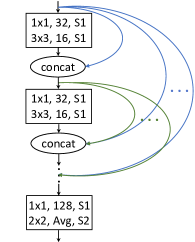
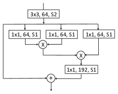
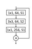
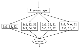
Our embedding module consists of a stem and a stack of three convolution blocks, gradually decreasing image resolution. The stem is a $3\times 3$ convolution followed by a max pooling of stride 2 (S2). The design of blocks is flexible, and we choose ResNet block [S-9], Inception block [S-24], DenseNet block [S-11] and Non-local block [S-29], whose configurations are shown in Fig. S-1. We halve the spatial size of feature maps for each block, and after the last block, we use a 1$\times$1 convolution to change the dimension of features such that the dimension is consistent with that of the backbone. For an input image of $224\times 224$, our token embedding outputs $14\times 14$ spatial features, reshaped to a sequence of 196 vectors as word tokens.

Backbone of transformer

We build the backbone by stacking standard transformer blocks as  [S-7], where each transformer block contains a multi-head self-attention (MSA) and a multi-layer perception (MLP). Throughout the backbone, the dimension of tokens (token size) remain unchanged. In MSA, we specify the number of heads; the dimension of queries, keys and values can be determined accordingly. Each MLP contains two fully-connected (FC) layers, where the dimension of hidden layer is increased (called MLP size).

Classification head

The proposed classification head combines the classification token and word tokens, where word tokens are aggregated by multi-headed global cross-covariance pooling (MGCrP) with structured normalization svPN. We keep the number of heads unchanged and vary the dimensions ($m$ and $n$) of two linear projections for SoT of different depths.

We develop a family of SoT, namely, a light-weight 12-layer SoT-Tiny, a middle-sized 14-layer SoT-Small and a heavyweight 24-layer SoT-Base, and their configurations are shown in Tab. S-1. In addition, to make computationally feasible the ablation analysis where extensive evaluations on ImageNet are involved, we also design a 7-layer SoT. It shares the same configuration with SoT-Tiny, but only has 7 layers and moreover, the downsampling of the last block in the token embedding module is removed.

		SoT-Tiny	SoT-Small	SoT-Base
Token embedding	Token size	240	384	528
Backbone	Layers	12	14	24
	MSA heads	4	6	8
	MLP size	600	1344	1584
Classification	MGCrP heads	6	6	6
head	MGCrP $(m,n)$	(14,14)	(24,24)	(38,38)
Parameters (M)		7.7	26.9	76.8
FLOPs (G)		2.5	5.8	14.5

Table S-1: Architectures of the proposed SoT networks.

(a) DenseNet block

(b) Non-local block

(c) ResNet block

(d) Inception block

Figure S-1: Illustration of different type of convolution blocks in our token embedding module. S1/2: Stride 1/2; Avg: average pooling; Max: max pooling.

B Proof of Proposition 1

Proposition 1.

Given $\mathbf{u}_{i}$ and $\mathbf{v}_{i}$ where $i=1,\ldots,k-1$, let us consider the objective

$$\max_{\|\mathbf{u}\|=\|\mathbf{v}\|=1}\; \mathbf{u}^{T}\mathbf{X}\mathbf{Y}^{T}\mathbf{v}$$ (S-1)

$$\mathrm{s.t.}\;\; \mathbf{u}_{i}^{T}\mathbf{u}=0,\;\mathbf{v}_{i}^{T}\mathbf{v}=0,\;i<k.$$

By inductively optimizing (S-1) for $k=1,\ldots,\min(m,n)$, we can obtain, in decreasing order, the $k$-th largest cross-covariance $\mathbf{u}_{k}^{T}\mathbf{X}\mathbf{Y}^{T}\mathbf{v}_{k}$, which is equal to the $k$-th singular value $\lambda_{k}$ of $\mathbf{Q}$ while $\mathbf{u}_{k}$ and $\mathbf{v}_{k}$ are the corresponding left and right singular vectors, respectively.

Proof.

We prove this proposition using mathematical induction. Note that $\mathbf{Q}=\mathbf{X}\mathbf{Y}^{T}$. For convenience, we let $R(\mathbf{Q},\mathbf{u},\mathbf{v})=\mathbf{u}^{T}\mathbf{X}\mathbf{Y}^{T}\mathbf{v}$.

Initial case First, let us consider the initial case of objective (S-1) for which $k=1$, i.e., $\max_{\|\mathbf{u}\|=\|\mathbf{v}\|=1}R(\mathbf{Q},\mathbf{u},\mathbf{v})$. Note that $\|\mathbf{u}\|=1$ is equivalent to $\|\mathbf{u}\|^{2}=\mathbf{u}^{T}\mathbf{u}=1$. The Lagrange function associated with the objective (S-1) is

$$\mathcal{L}(\mathbf{u},\mathbf{v},\gamma,\beta)=R(\mathbf{Q},\mathbf{u},\mathbf{v})-\dfrac{\gamma}{2}(\mathbf{u}^{T}\mathbf{u}-1)-\dfrac{\beta}{2}(\mathbf{v}^{T}\mathbf{v}-1).$$ (S-2)

We calculate the gradient $\triangledown\mathcal{L}=\Big{[}\frac{\partial\mathcal{L}}{\partial\mathbf{u}},\frac{\partial\mathcal{L}}{\partial\mathbf{v}},\frac{\partial\mathcal{L}}{\partial\gamma},\frac{\partial\mathcal{L}}{\partial\beta}\Big{]}$, where $\frac{\partial\mathcal{L}}{\partial\mathbf{u}}$ is the partial derivatives of $\mathcal{L}$ with respect to $\mathbf{u}$, and set it to be zero. After some manipulations, we have

$$\mathbf{Q}\mathbf{v}-\gamma\mathbf{u}=0,$$ (S-3)

$$\mathbf{Q}^{T}\mathbf{u}-\beta\mathbf{v}=0,$$

$$\mathbf{u}^{T}\mathbf{u}-1=0,$$

$$\mathbf{v}^{T}\mathbf{v}-1=0.$$

The last two equations simply produce the constraints, i.e., $\|\mathbf{u}\|=1$ and $\|\mathbf{v}\|=1$. We left multiple the first and second equation by $\mathbf{u}^{T}$ and $\mathbf{v}^{T}$, respectively. Then we can obtain

$$\gamma=\beta=R(\mathbf{Q},\mathbf{u},\mathbf{v}),$$

as $\mathbf{u}^{T}\mathbf{Q}\mathbf{v}=\mathbf{v}^{T}\mathbf{Q}^{T}\mathbf{u}$. Therefore, we have

$$\mathbf{Q}\mathbf{v}=\gamma\mathbf{u},$$ (S-4)

$$\mathbf{Q}^{T}\mathbf{u}=\gamma\mathbf{v}.$$

According to the property of SVD [S-8, Chap.2.4], we know that $\mathbf{u}$ and $\mathbf{v}$ which satisfy S-4 are respectively left and right singular vectors of $\mathbf{Q}$ with $\gamma$ being the singular value. Obviously, $R(\mathbf{Q},\mathbf{u},\mathbf{v})$ achieves its maximum when it is equal to the largest singular value. Therefore, by optimizing the objective (S-1) with $k=1$, we obtain vectors $\mathbf{u}_{1}$ and $\mathbf{v}_{1}$ which are respectively the left and right singular vectors corresponding to the largest singular value $\lambda_{1}=R(\mathbf{Q},\mathbf{u}_{1},\mathbf{v}_{1})$.

Inductive step Next, we optimize the objective (S-1) for $k>1$. Suppose the statement holds for $i<k$. That is, for any $i$, $\mathbf{u}_{i}$ and $\mathbf{v}_{i}$, which maximize $R(\mathbf{Q},\mathbf{u},\mathbf{v})$ while satisfying the constraints $\|\mathbf{u}_{i}\|=\|\mathbf{v}_{i}\|=1$ and $\mathbf{u}_{i}^{T}{\mathbf{u}_{i^{\prime}}}=0,\mathbf{v}_{i}^{T}{\mathbf{v}_{i^{\prime}}}=0,i^{\prime}<i$, are the singular vectors corresponding to the $i\mathrm{th}$ largest singular values $\lambda_{i}$. Obviously

$$\underbrace{R(\mathbf{Q},\mathbf{u}_{1},\mathbf{v}_{1})}_{\lambda_{1}}\geq\ldots\geq\underbrace{R(\mathbf{Q},\mathbf{u}_{k-1},\mathbf{v}_{k-1})}_{\lambda_{k-1}}.$$

Now, let us prove the statement holds for the case $k$. The Lagrange function of the objective (S-1) is

$$\mathcal{L}( \mathbf{u},\mathbf{v},\gamma,\beta,\tau_{i},\delta_{i})=R(\mathbf{Q},\mathbf{u},\mathbf{v})-\dfrac{\gamma}{2}(\mathbf{u}^{T}\mathbf{u}-1)$$ (S-5)

$$-\dfrac{\beta}{2}(\mathbf{v}^{T}\mathbf{v}-1)-\sum\nolimits_{i=1}^{k-1}\tau_{i}\mathbf{u}^{T}\mathbf{u}_{i}-\sum\nolimits_{i=1}^{k-1}\delta_{i}\mathbf{v}^{T}\mathbf{v}_{i}.$$

We calculate the gradient of the Lagrange function $\triangledown\mathcal{L}=\Big{[}\frac{\partial\mathcal{L}}{\partial\mathbf{u}},\frac{\partial\mathcal{L}}{\partial\mathbf{v}},\frac{\partial\mathcal{L}}{\partial\gamma},\frac{\partial\mathcal{L}}{\partial\beta},\frac{\partial\mathcal{L}}{\partial\tau_{1}},\ldots,\frac{\partial\mathcal{L}}{\partial\tau_{k-1}},\frac{\partial\mathcal{L}}{\partial\delta_{1}},\ldots,\frac{\partial\mathcal{L}}{\partial\delta_{k-1}}\Big{]}$. By setting $\triangledown\mathcal{L}$ to be zero, we obtain a set of equations

$$\mathbf{Q}\mathbf{v}-\gamma\mathbf{u}-\sum\nolimits_{i=1}^{k-1}\tau_{i}\mathbf{u}_{i}=0,$$ (S-6)

$$\mathbf{Q}^{T}\mathbf{u}-\beta\mathbf{v}-\sum\nolimits_{i=1}^{k-1}\delta_{i}\mathbf{v}_{i}=0,$$

$$\mathbf{u}^{T}\mathbf{u}-1=0,$$

$$\mathbf{v}^{T}\mathbf{v}-1=0,$$

$$\mathbf{u}^{T}\mathbf{u}_{i}=0,\;i=1,\ldots,k-1,$$

$$\mathbf{v}^{T}\mathbf{v}_{i}=0,\;i=1,\ldots,k-1.$$

The third to last equations are simply constraints of the maximization problem (S-1). We left multiply $\mathbf{u}^{T}$ (resp., $\mathbf{v}^{T}$) the first (resp., second) equation, and we can obtain $\mathbf{u}^{T}\mathbf{Q}\mathbf{v}=\gamma$ (resp., $\mathbf{\mathbf{v}}^{T}\mathbf{Q}^{T}\mathbf{u}=\beta$), by noting that $\mathbf{u}^{T}\mathbf{u}_{i}=0$ (resp., $\mathbf{v}^{T}\mathbf{v}_{i}=0$) $\mathbf{u}$ for $i<k$. Therefore, we have $\gamma=\beta=R(\mathbf{Q},\mathbf{u},\mathbf{v})$.

Subsequently, we will show that $\tau_{j}=0,j<k$. We left multiply the first equation by $\mathbf{u}_{j}^{T},j<k$. We recall that $\mathbf{u}_{j}$ is orthogonal to $\mathbf{u}_{j^{\prime}}$ for $j^{\prime}\neq j$ and to $\mathbf{u}$, and then can derive

$$\tau_{j}=\mathbf{u}_{j}^{T}\mathbf{Q}\mathbf{v}.$$

As $\mathbf{u}_{j}$ is the left singular value of $\mathbf{Q}$, we know $\mathbf{Q}^{T}\mathbf{u}_{j}=\lambda_{j}\mathbf{v}_{j}$, i.e., $\mathbf{u}_{j}^{T}\mathbf{Q}=\lambda_{j}\mathbf{v}_{j}$. Therefore we have

$$\tau_{j}=\mathbf{u}_{j}^{T}\mathbf{Q}\mathbf{v}=\lambda_{j}\mathbf{v}_{j}^{T}\mathbf{v}=0.$$

Here we make use of the fact that $\mathbf{v}_{j}$ is orthogonal to $\mathbf{v}$. In a similar manner, we left multiply the second equation by $\mathbf{v}_{j}^{T},j<k$, and then we can derive $\delta_{j}=0$. Up to this point, we know $\mathbf{u}$ and $\mathbf{v}$ for which the objective (S-1) is maximized satisfy the following pair of equations

$$\mathbf{Q}\mathbf{v}=\gamma\mathbf{u},$$ (S-7)

$$\mathbf{Q}^{T}\mathbf{u}=\gamma\mathbf{v}.$$

Again, according to the property of SVD, we know $\mathbf{u}$ and $\mathbf{v}$ are left and right singular values of $\mathbf{Q}$ and $\gamma$ is the corresponding singular value. Obviously, $\gamma$ achieves the maximum when it equals the $k$-$\mathrm{th}$ largest singular value. This concludes our proof. ∎

As far as we know, the statement as described in Proposition 1 appeared early in [S-2] and later in [S-27, Chap. 14.1.7], among others. However, we fail to find any formal proof of this statement; hence, we provide a proof here. It is worth mentioning that this statement is closely related to but different from canonical correlation analysis (CCA). For detailed theory on CCA, one may refer to [S-26].

C Backpropagation of svPN via SVD

Let $\mathbf{Q}=\mathbf{U}\mathrm{diag}(\lambda_{i})\mathbf{V}^{T}$ be the SVD of $\mathbf{Q}$. The forward propagation of our normalization $\tilde{\mathbf{Q}}\stackrel{{\scriptstyle\vartriangle}}{{=}}\mathrm{svPN}(\mathbf{Q})$ can be described in two consecutive steps as follows:

$$\mathbf{Q}\stackrel{{\scriptstyle\;\mathrm{SVD}\;}}{{\longrightarrow}}\mathbf{U}\mathrm{diag}(\lambda_{i})\mathbf{V}^{T}\stackrel{{\scriptstyle\mathrm{power}\;}}{{\longrightarrow}}\mathbf{U}\mathrm{diag}(\lambda_{i}^{\alpha})\mathbf{V}^{T}$$ (S-8)

The associated backward propagations are not that straightforward as the structured, nonlinear matrix operations are involved. Suppose $l$ is the network loss function. Let us denote $\mathbf{A}_{\mathrm{sym}}=\frac{1}{2}(\mathbf{A}+\mathbf{A}^{T})$, $\mathbf{\Lambda}=\mathrm{diag}(\lambda_{i})$, and $\mathbf{A}_{\mathrm{diag}}$ being a matrix setting the off-diagonals of $\mathbf{A}$ to zero. Based on the theory of matrix backpropagation [S-12], we can derive the gradients relative to $\mathrm{svPN}$ via SVD, which are given in the following corollary.

Corollary 1.

Suppose we have $\dfrac{\partial l}{\partial\tilde{\mathbf{Q}}}$ from the succeeding layer. The gradient involved in the first step of (S-8) is

$$\dfrac{\partial l}{\partial\mathbf{Q}}=\dfrac{\partial l}{\partial\mathbf{U}}\mathbf{\Lambda}^{-1}\mathbf{V}^{T}+\mathbf{U}\Big{(}\dfrac{\partial l}{\partial\mathbf{\Lambda}}-\mathbf{U}^{T}\dfrac{\partial l}{\partial\mathbf{U}}\mathbf{\Lambda}^{-1}\Big{)}_{\mathrm{diag}}\mathbf{V}^{T}$$

$$+2\mathbf{U}\mathbf{\Lambda}\Big{(}\mathbf{K}^{T}\circ\Big{(}\mathbf{V}^{T}\Big{(}\dfrac{\partial l}{\partial\mathbf{V}}-\mathbf{V}\mathbf{\Lambda}^{-1}\Big{(}\dfrac{\partial l}{\partial\mathbf{U}}\Big{)}^{T}\mathbf{U}\mathbf{\Lambda}\Big{)}\Big{)}\Big{)}_{\mathrm{sym}}\mathbf{V}^{T}$$

where $K_{ij}=(\lambda_{i}^{2}-\lambda_{j}^{2})^{-1}$ if $\lambda_{i}\neq\lambda_{j}$ and $K_{ij}=0$ otherwise, and $\circ$ denotes Hadamard product. The partial derivatives with respect to the second step of (S-8) are

$$\dfrac{\partial l}{\partial\mathbf{U}} =\dfrac{\partial l}{\partial\tilde{\mathbf{Q}}}\mathbf{V}\mathbf{\Lambda}^{\alpha},$$

$$\dfrac{\partial l}{\partial\mathbf{V}} =\Big{(}\dfrac{\partial l}{\partial\tilde{\mathbf{Q}}}\Big{)}^{T}\mathbf{U}\mathbf{\Lambda}^{\alpha},$$

$$\dfrac{\partial l}{\partial\mathbf{\Lambda}} =\alpha\mathbf{\Lambda}^{\alpha-1}\mathbf{U}^{T}\dfrac{\partial l}{\partial\tilde{\mathbf{Q}}}\mathbf{V}.$$

D Detailed Experimental Settings for CV and NLP Tasks

D.1 Benchmark Description

D.1.1 Benchmarks Used in CV

ImageNet Our experiments are mainly conducted on ILSVRC ImageNet 2012 image classification benchmark [S-21,S-5], which contains 1K classes with 1.28M images for training and 50K images for validation. Note that as test images are not publicly available, the common practice is to adopt the validation images for testing [S-34,S-25,S-35]. We train the transformer models from scratch on the training set and report top-1 accuracy on the validation set.

Figure S-2: Examples of adversarial images from ImageNet-A (1st column). The blue text is the test class, and the red text is the false prediction and the score produced by a DeiT-Small model. The 2nd and 3rd columns show the images of the corresponding classes from ImageNet. It can be seen that the images from ImageNet-A are highly adversarial, whose distribution deviates much from that of ImageNet. On the challenging ImageNet-A, the proposed method can substantially improve state-of-the-art vision transformers (see Sec. 4.2.3 in the main paper).

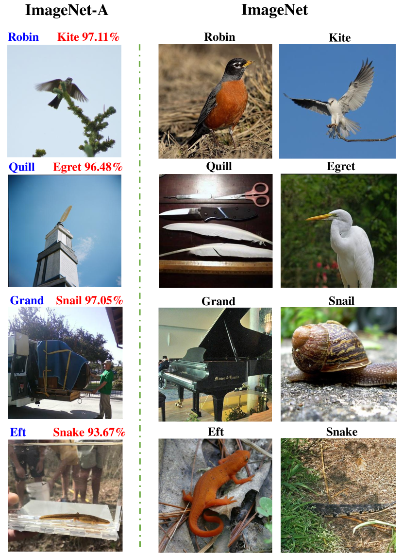
ImageNet-A The ImageNet-A [S-10] is a hard ImageNet test set of real-world adversarial images with adversarial filtration. It contains 7,500 natural images from 200 classes which cover most broad categories spanned by ImageNet. This dataset has heterogeneous and varied distribution shift from ImageNet. ImageNet-A is far more challenging than the original ImageNet validation set (and test set). For example, DeiT-Small model achieves only a top-1 accuracy of 18.9% on ImageNet-A against 79.8% on ImageNet validation set. Fig. S-2 (1st column) shows four examples from ImageNet-A, in which an object (blue text) of some class is mistakenly identified as that of another class with high confidence score (in red); for contrast, the 2nd and 3rd columns show the images of the corresponding classes in ImageNet. It can be seen that images of ImageNet-A is highly adversarial and its distribution deviates much from that of ImageNet. Notably, on the challenging ImageNet-A, the proposed method can substantially improve state-of-the-art vision transformers (see Sec. 4.2.3 in the main paper).

D.1.2 Benchmarks Used in NLP

CoLA  The goal of the Corpus of Linguistic Acceptability task [S-30] is to judge whether a sentence is grammatical or not. It can be formulated as a binary single-sentence classification problem. The dataset contains 10,657 English sentences which are labeled as grammatical or ungrammatical, and these sentences are split into training (8,551)/development (1,043)/test (1,063) sets.

RTE  Given a pair of text fragments, denoted by (“Text”, “Hypothesis”), Recognizing Textual Entailment [S-1] aims to determine whether the “Text” entails “Hypothesis”. This task can be converted into a binary entailment classification task. The dataset of RTE consists of 5,767 examples, among which the training set contains 2,490 examples, while the development set and test set contain 3,000 and 277 examples, respectively.

(a) Sentence-pair classification task (RTE, MNLI and QNLI).

(b) Single-sentence classification task (CoLA)

Figure S-3: Diagrams of fine-tuning BERT and GPT on downstream NLP tasks, formulated as either (a) sentence-pair classification (RTE, MNLI and QNLI), or (b) single-sentence classification (CoLA). Note that for BERT & its variants, the classification token [CLS] is always in the first place of the sequence, while it is at the end for GPT whose illustration fades; besides, GPT does not use segment embedding.

Models	SoT-Tiny	SoT-Small	SoT-Base
Batch size	1024	1024	512
Optimizer	AdamW	AdamW	AdamW
Epochs	310	310	310
Base LR	1e-3	1e-3	5e-4
Final LR	1e-5	1e-5	1e-5
Scheduler	cosine	cosine	cosine
Weight decay	0.03	0.03	0.065
Label smoothing	0.1	0.1	0.1
Mixup prob.	0.8	0.8	0.8
Cutmix prob.	1.0	1.0	1.0
Erasing prob.	0.25	0.25	0.25
RandAugment	9/0.5	9/0.5	9/0.5
MGCrP dropout	0.0	0.5	0.7

Table S-2: Hyper-parameters for image classification.

MNLI  Similar to RTE, Multi-Genre Natural Language Inference [S-31] is also concerned with judgement of entailment. Given a pair of sentences, the task is to predict whether the “Text” entails the “Hypothesis” (entailment), contradicts the “Hypothesis” (contradiction), or neither (neutral). As such, this task can be formulated as a three-way classification problem. MNLI is a large-scale dataset, consisting of 432,702 examples, in which 392,702 examples belong to the training set, 20,000 examples belong to the development set and the remaining 20,000 examples are in the test set.

QNLI  The Stanford Question Answering task [S-20] is converted to a sentence-pair classification problem [S-28]. Given a pair of sentences, the model needs to determine whether the sentence contains the answer to the question. QNLI dataset contains 105K training examples, 5.4K development examples and 5.4K test examples.

D.2 Training Strategy

D.2.1 Training from Scratch on CV Tasks

As suggested in [S-7], training of high-performance transformer models requires ultra large-scale datasets. Hence, for training from scratch on ImageNet which is not that large, one often depends on extensive data augmentation and regularization methods [S-25], for which we mainly follow  [S-25,S-34,S-35]. For data augmentation, besides standard scale, color and flip jittering [S-14,S-9] with default settings in PyTorch, we adopt randAugment [S-4] and random erasing [S-39]. For model regularization, we employ label smoothing [S-23], mixup [S-38] and cutmix [S-36]. We use AdamW [S-17] optimizer with a learning rate warm up (5 epochs) and cosine annealing scheduler. We adopt dropout for our MGCrP module. The hyper-parameters involved in augmentation, regularization, optimization, etc., are summarized in Tab. S-2. Note that the 7-layer SoT used in the ablation study shares the same hyper-parameters with SoT-Tiny.

Models		GPT	BERT	SpanBERT	RoBERTa
Batch size		{32,64}	{24,64,96}	32	{16,32}
Adam	$\beta_{1}$	0.9	0.9	0.9	0.9
Optimizer	$\beta_{2}$	0.999	0.999	0.999	0.98
	$\epsilon$	1e-8	1e-8	1e-6	1e-6
Epochs		{10,15}	10	{10,30}	{10,20}
Base LR		6.25e-5	{2e-5,3e-5}	2e-5	{1e-5,2e-5}
Final LR		0	0	0	0
Scheduler		linear	linear	linear	linear
Weight decay		0.01	0	0.01	0.1
MGCrP repr. size		{4K,6K}	{1K,4K,5K}	{1K,4K,5K}	{1K,4K,5K}
MGCrP dropout		{0.5,0.7}	{0.5,0.8}	{0.5,0.7}	{0.5,0.7}

Table S-3: Hyper-parameters for text classification.

D.2.2 Fine-tuning on Downstream NLP Tasks

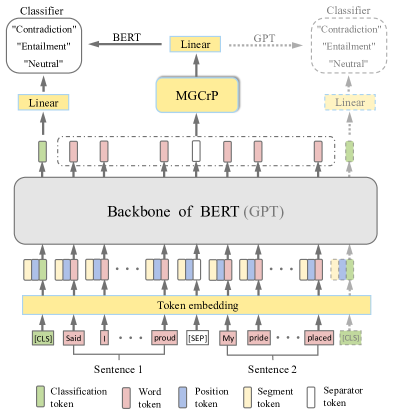
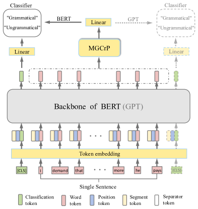
The illustration of fine-tuning BERT and GPT with our classification head can be seen in Fig S-3. The four NLP tasks are formulated as either sentence-pair classification task (RTE, MNLI and QNLI) or single-sentence classification task (CoLA). For each task, we plug in the task-specific input and outputs into the transformer models and fine-tune the whole networks in an end-to-end fashion. Following previous works [S-16,S-19,S-6,S-13], for each task we fine-tune the model on the training set while evaluating on the development set.

In the following, we introduce the fine-tuning pipeline by taking the sentence-pair classification with BERT model as an example. As shown in Fig. 3(a), for a sentence-pair classification, a pair of sentences are concatenated into a single sequence with a special token ([$\mathrm{SEP}$]) separating them, and is then prepended by a classification token ([$\mathrm{CLS}$]). The input representation of every token is built by summing the word embedding (by e.g., WordPiece [S-33]), segment embedding and position embedding. At the output, the token representations are fed into our proposed classification head, in which we combine classification token and word tokens. Fig. 3(b) shows the single-sentence classification task, which is similar to sentence-pair task except the input only involves one sentence. We mention that the [$\mathrm{CLS}$] is always in the first place of the token sequence for BERT, while in the last for GPT.

For GPT and BERT & its variants, most training strategies and hyper-parameters in fine-tuning are the same as those in pre-training. We use Adam [S-15] algorithm for model optimization. The learning rate is linearly warmed up over a number of steps to a peak value, and then linearly decayed to zero. We mainly tune the batch size, learning rate and number of training epochs. The optimal hyper-parameters are task-specific. Following [S-19,S-6], we choose them from a small set of options; for example, for GPT, we select batch size from {32,64}. For our classification head, we use dropout for MGCrP. For simplicity, we adopt single head for our MGCrP and select the representation (repr.) size from a set of values, e.g., {4K,6K} for GPT. The detailed settings of the hyper-parameters are summarized in Tab. S-3.

Fine-tuning of BERT and GPT are implemented based on HuggingFace’s codebase [S-32], while that of RoBERTa is based on fairseq [S-18], an open-source sequence modeling toolkit. We implement fine-tuning of SpanBERT using the code available at official website of facebook. The pretrained BERT model is downloaded from HuggingFace’s website, and pretrained RoBERTa and SpanBERT models are both from fairseq website. The pretrained GPT model is available at the official website of OpenAI .

Figure S-4: Visualizations of images on ImageNet validation set based on SoT-Tiny by using the Grad-CAM [S-22]. We show the examples for which ClassT+WordT predicts correctly, but ClassT or WordT fails. ✓: correct prediction; ✗: incorrect prediction.

Figure S-5: Visualization of the influence of each word for linguistic acceptability on the given English sentence. We adopt the BERT-base as the backbone and refer [S-37,S-3] to obtain the results. ✓: correct prediction; ✗: incorrect prediction.

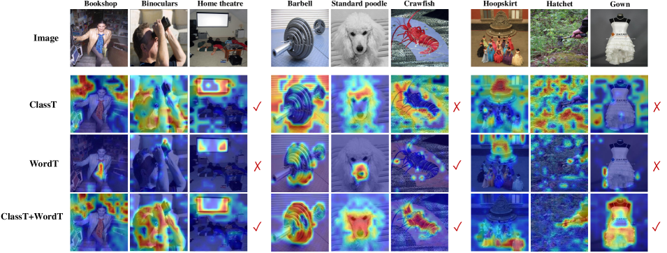
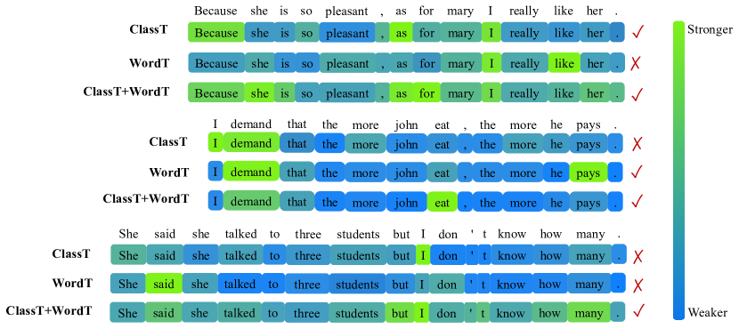
E Visualization for CV and NLP Tasks

To further analyze the effectiveness of our proposed classification head, we make qualitative comparisons by visualizing the models for CV and NLP tasks. Specifically, SoT-Tiny and the BERT-base are used as the backbone models for CV and NLP tasks, respectively. For each model, we compare three variants as follows:

• ClassT: only classification token is used for classifier;

• WordT: only word tokens are used for classifier;

• ClassT+WordT: Both classification token and word tokens are used for classifier based on the sum scheme.

E.1 Visualization for CV Model

To visualize the models in CV task, we first train our SoT-Tiny variants on ImageNet, and then adopt the Grad-CAM [S-22] to obtain class activation map of each input image. As such, we can visualize the most important regions (i.e., regions of interest) for the final classification according to the gradient information. As illustrated in Fig. S-4, we show three kinds of scenarios, in which ClassT+WordT all makes correct predictions, i.e., (left panel) ClassT makes correct predictions but WordT fails, (middle panel) WordT predicts correctly but ClassT does not; (right panel) neither ClassT nor WordT predicts correctly.

From Fig. S-4, we have the following observations: (1) As classification token interacts with all word tokens across the network, it tends to focus on the global context of images, especially some messy backgrounds. Therefore, ClassT is more suitable for classifying the categories associated with the backgrounds and the whole context, e.g., “Bookshop”. (2) The word tokens mainly correspond to local patches, so WordT performs classification primarily based on some local discriminative regions. As such, WordT has better ability to classify the categories associated with local parts and subtle variations, e.g., “Standard poodle”. (3) Our ClassT+WordT can make fully use of merits of both word tokens and classification token, which can focus on the most important regions for better classification by exploiting both local discriminative parts and global context information.

E.2 Visualization for NLP Model

Similarly, we compare the visualization results of the BERT-base under three scenarios on the examples of CoLA. The task is to judge whether an English sentence is grammatical or not. We use visualization methods proposed in [S-37,S-3] to show the influence of each word in the final prediction. As shown in Fig. S-5, the green denotes stronger impact while the blue implies weaker one.

All examples in Fig. S-5 are ungrammatical. Overall, we can see ClassT inclines to make predictions from the whole sentence, such as the conjunction of two sub-sentences (e.g., “Because.., as”) or the key global semantic word; WordT tends to focus on local correctness of each sentence, ignoring the global context. This observation is similar with the visualization results of CV model, demonstrating that the classification token and word tokens are highly complementary for both CV and NLP tasks. Finally, the proposed ClassT+WordT can highlight all important words in sentence, including the subordinate clause, conjunction, etc., which can help to boost the performance of classification.

ieee_fullname

References

- [1] Irwan Bello. Lambdanetworks: Modeling long-range interactions without attention. In ICLR, 2020.
- [2] Luisa Bentivogli, Peter Clark, Ido Dagan, and Danilo Giampiccolo. The fifth pascal recognizing textual entailment challenge. In TAC, 2009.
- [3] Christopher Bishop. Pattern Recognition and Machine Learning. Springer, 2006.
- [4] Minghao Chen, Houwen Peng, Jianlong Fu, and Haibin Ling. Autoformer: Searching transformers for visual recognition. In ICCV, 2021.
- [5] Ekin D Cubuk, Barret Zoph, Jonathon Shlens, and Quoc V Le. Randaugment: Practical automated data augmentation with a reduced search space. In CVPR, 2020.
- [6] Jia Deng, Wei Dong, Richard Socher, Li-Jia Li, Kai Li, and Li Fei-Fei. ImageNet: A large-scale hierarchical image database. In CVPR, 2009.
- [7] Jacob Devlin, Ming-Wei Chang, Kenton Lee, and Kristina Toutanova. BERT: pre-training of deep bidirectional transformers for language understanding. In NAACL-HLT, 2019.
- [8] Alexey Dosovitskiy, Lucas Beyer, Alexander Kolesnikov, Dirk Weissenbor, Xiaohua Zhai, Thomas Unterthiner, Mostafa Dehghani, Matthias Minderer, Georg Heigold, Sylvain Gelly, Jakob Uszkoreit, and Neil Houlsby. An image is worth 16x16 words: Transformers for image recognition at scale. In ICLR, 2021.
- [9] Jonas Gehring, Michael Auli, David Grangier, Denis Yarats, and Yann N. Dauphin. Convolutional sequence to sequence learning. In ICML, 2017.
- [10] Arthur Gretton, Michael W Mahoney, Mehryar Mohri, and Ameet S Talwalkar. Low-rank methods for large-scale machine learning. In NIPS Workshop, 2010.
- [11] Kai Han, Yunhe Wang, Hanting Chen, Xinghao Chen, Jianyuan Guo, Zhenhua Liu, Yehui Tang, An Xiao, Chunjing Xu, Yixing Xu, Zhaohui Yang, Yiman Zhang, and Dacheng Tao. A survey on visual transformer. arXiv preprint arXiv:2012.12556, 2020.
- [12] Kaiming He, Xiangyu Zhang, Shaoqing Ren, and Jian Sun. Deep residual learning for image recognition. In CVPR, 2016.
- [13] Dan Hendrycks, Kevin Zhao, Steven Basart, Jacob Steinhardt, and Dawn Song. Natural adversarial examples. In CVPR, 2021.
- [14] Byeongho Heo, Sangdoo Yun, Dongyoon Han, Sanghyuk Chun, Junsuk Choe, and Seong Joon Oh. Rethinking spatial dimensions of vision transformers. In ICCV, 2021.
- [15] Sepp Hochreiter and Jürgen Schmidhuber. Long short-term memory. Neural computation, 9(8):1735–1780, 1997.
- [16] Gao Huang, Zhuang Liu, Laurens van der Maaten, and Kilian Q. Weinberger. Densely connected convolutional networks. In CVPR, 2017.
- [17] Catalin Ionescu, Orestis Vantzos, and Cristian Sminchisescu. Matrix backpropagation for deep networks with structured layers. In ICCV, 2015.
- [18] Geoffrey E. Hinton Jimmy Lei Ba, Jamie Ryan Kiros. Layer normalization. arXiv:1607.06450, 2016.
- [19] Mandar Joshi, Danqi Chen, Yinhan Liu, Daniel S Weld, Luke Zettlemoyer, and Omer Levy. SpanBERT: Improving pre-training by representing and predicting spans. TACL, 8:64–77, 2020.
- [20] Andrew Zisserman Karen Simonyan. Very deep convolutional networks for large-scale image recognition. In ICLR, 2015.
- [21] Salman H. Khan, Muzammal Naseer, Munawar Hayat, Syed Waqas Zamir, Fahad Shahbaz Khan, and Mubarak Shah. Transformers in vision: A survey. arXiv preprint arXiv:2101.01169, 2021.
- [22] Alex Krizhevsky, Ilya Sutskever, and Geoffrey E Hinton. Imagenet classification with deep convolutional neural networks. In NIPS, 2012.
- [23] Peihua Li, Jiangtao Xie, Qilong Wang, and Zilin Gao. Towards faster training of global covariance pooling networks by iterative matrix square root normalization. In CVPR, 2018.
- [24] Peihua Li, Jiangtao Xie, Qilong Wang, and Wangmeng Zuo. Is second-order information helpful for large-scale visual recognition? In ICCV, 2017.
- [25] Min Lin, Qiang Chen, and Shuicheng Yan. Network in network. In ICLR, 2014.
- [26] Tsung-Yu Lin, Aruni Roy Chowdhury, and Subhransu Maji. Bilinear convolutional neural networks for fine-grained visual recognition. IEEE TPAMI, 40(6):1309–1322, 2018.
- [27] Tsung-Yu Lin and Subhransu Maji. Improved bilinear pooling with CNNs. In BMVC, 2017.
- [28] Tsung-Yu Lin, Aruni RoyChowdhury, and Subhransu Maji. Bilinear CNN models for fine-grained visual recognition. In ICCV, 2015.
- [29] Yinhan Liu, Myle Ott, Naman Goyal, Jingfei Du, Mandar Joshi, Danqi Chen, Omer Levy, Mike Lewis, Luke Zettlemoyer, and Veselin Stoyanov. RoBERTa: A robustly optimized bert pretraining approach. arXiv preprint arXiv:1907.11692, 2019.
- [30] Ze Liu, Yutong Lin, Yue Cao, Han Hu, Yixuan Wei, Zheng Zhang, Stephen Lin, and Baining Guo. Swin transformer: Hierarchical vision transformer using shifted windows. In ICCV, 2021.
- [31] Ilya Loshchilov and Frank Hutter. Decoupled weight decay regularization. In ICLR, 2018.
- [32] Zhiliang Peng, Wei Huang, Shanzhi Gu, Lingxi Xie, Yaowei Wang, Jianbin Jiao, and Qixiang Ye. Conformer: Local features coupling global representations for visual recognition. In ICCV, 2021.
- [33] Alec Radford, Karthik Narasimhan, Tim Salimans, and Ilya Sutskever. Improving language understanding by generative pre-training. Technical report, OpenAI, 2018.
- [34] Alec Radford, Jeffrey Wu, Rewon Child, David Luan, Dario Amodei, and Ilya Sutskever. Language models are unsupervised multitask learners. Technical report, OpenAI, 2019.
- [35] Pranav Rajpurkar, Jian Zhang, Konstantin Lopyrev, and Percy Liang. Squad: 100,000+ questions for machine comprehension of text. In EMNLP, pages 2383–2392, 2016.
- [36] Olga Russakovsky, Jia Deng, Hao Su, Jonathan Krause, Sanjeev Satheesh, Sean Ma, Zhiheng Huang, Andrej Karpathy, Aditya Khosla, Michael Bernstein, Alexander C. Berg, and Li Fei-Fei. ImageNet Large Scale Visual Recognition Challenge. IJCV, 115(3):211–252, 2015.
- [37] Seymour Shlien. A method for computing the partial singular value decomposition. IEEE TPAMI, 4(6):671–676, 1982.
- [38] Chen Sun, Abhinav Shrivastava, Saurabh Singh, and Abhinav Gupta. Revisiting unreasonable effectiveness of data in deep learning era. In CVPR, 2017.
- [39] Christian Szegedy, Wei Liu, Yangqing Jia, Pierre Sermanet, Scott Reed, Dragomir Anguelov, Dumitru Erhan, Vincent Vanhoucke, and Andrew Rabinovich. Going deeper with convolutions. In CVPR, 2015.
- [40] Hugo Touvron, Matthieu Cord, Matthijs Douze, Francisco Massa, Alexandre Sablayrolles, and Herve Jegou. Training data-efficient image transformers & distillation through attention. In ICML, 2021.
- [41] Ashish Vaswani, Noam Shazeer, Niki Parmar, Jakob Uszkoreit, Llion Jones, Aidan N Gomez, Lukasz Kaiser, and Illia Polosukhin. Attention is all you need. In NIPS, 2017.
- [42] Qilong Wang, Jiangtao Xie, Wangmeng Zuo, Lei Zhang, and Peihua Li. Deep CNNs meet global covariance pooling: Better representation and generalization. IEEE TPAMI, 43(8):2582–2597, 2021.
- [43] Qilong Wang, Li Zhang, Banggu Wu, Dongwei Ren, Peihua Li, Wangmeng Zuo, and Qinghua Hu. What deep cnns benefit from global covariance pooling: An optimization perspective. In CVPR, 2020.
- [44] Wenhai Wang, Enze Xie, Xiang Li, Deng-Ping Fan, Kaitao Song, Ding Liang, Tong Lu, Ping Luo, and Ling Shao. Pyramid vision transformer: A versatile backbone for dense prediction without convolutions. In ICCV, 2021.
- [45] Xiaolong Wang, Ross Girshick, Abhinav Gupta, and Kaiming He. Non-local neural networks. In CVPR, 2018.
- [46] Alex Warstadt, Amanpreet Singh, and Samuel R Bowman. Neural network acceptability judgments. TACL, pages 625–641, 2019.
- [47] Adina Williams, Nikita Nangia, and Samuel R Bowman. A broad-coverage challenge corpus for sentence understanding through inference. In NAACL-HLT, 2018.
- [48] Kan Wu, Houwen Peng, Minghao Chen, Jianlong Fu, and Hongyang Chao. Rethinking and improving relative position encoding for vision transformer. In ICCV, 2021.
- [49] Yoshua Bengio Patrick Haffner Yann LeCun, Léon Bottou. Gradient-based learning applied to document recognition. Proceedings of the IEEE, 86(11):2278–2324, 1998.
- [50] Tan yu, Yunfeng Cai, and Ping Li. Toward faster and simpler matrix normalization via rank-1 update. In ECCV, 2020.
- [51] Li Yuan, Yunpeng Chen, Tao Wang, Weihao Yu, Yujun Shi, Francis EH Tay, Jiashi Feng, and Shuicheng Yan. Tokens-to-token ViT: Training vision transformers from scratch on imagenet. In ICCV, 2021.
- [52] Xiaoyu Yue, Shuyang Sun, Zhanghui Kuang, Meng Wei, Philip Torr, Wayne Zhang, and Dahua Lin. Vision transformer with progressive sampling. In ICCV, 2021.
- [53] Sangdoo Yun, Dongyoon Han, Seong Joon Oh, Sanghyuk Chun, Junsuk Choe, and Youngjoon Yoo. Cutmix: Regularization strategy to train strong classifiers with localizable features. In ICCV, 2019.
- [54] Hongyi Zhang, Moustapha Cisse, Yann N. Dauphin, and David Lopez-Paz. Mixup: Beyond empirical risk minimization. ICLR, 2018.
- [S-1] Luisa Bentivogli, Peter Clark, Ido Dagan, and Danilo Giampiccolo. The fifth pascal recognizing textual entailment challenge. In TAC, 2009.
- [S-2] Christopher S. Bretherton, Catherine Smith, and John M. Wallace. An intercomparison of methods for finding coupled patterns in climate data. JCLI, (6):541–560, 1992.
- [S-3] Hila Chefer, Shir Gur, and Lior Wolf. Transformer interpretability beyond attention visualization. arXiv preprint arXiv:2012.09838, 2021.
- [S-4] Ekin D Cubuk, Barret Zoph, Jonathon Shlens, and Quoc V Le. Randaugment: Practical automated data augmentation with a reduced search space. In CVPR, 2020.
- [S-5] Jia Deng, Wei Dong, Richard Socher, Li-Jia Li, Kai Li, and Li Fei-Fei. ImageNet: A large-scale hierarchical image database. In CVPR, 2009.
- [S-6] Jacob Devlin, Ming-Wei Chang, Kenton Lee, and Kristina Toutanova. BERT: pre-training of deep bidirectional transformers for language understanding. In NAACL-HLT, 2019.
- [S-7] Alexey Dosovitskiy, Lucas Beyer, Alexander Kolesnikov, Dirk Weissenbor, Xiaohua Zhai, Thomas Unterthiner, Mostafa Dehghani, Matthias Minderer, Georg Heigold, Sylvain Gelly, Jakob Uszkoreit, and Neil Houlsby. An image is worth 16x16 words: Transformers for image recognition at scale. In ICLR, 2021.
- [S-8] Gene H. Golub and Charles F. Van Loan. Matrix Computations (4th Ed.). Johns Hopkins University Press, USA, 2003.
- [S-9] Kaiming He, Xiangyu Zhang, Shaoqing Ren, and Jian Sun. Deep residual learning for image recognition. In CVPR, 2016.
- [S-10] Dan Hendrycks, Kevin Zhao, Steven Basart, Jacob Steinhardt, and Dawn Song. Natural adversarial examples. In CVPR, 2021.
- [S-11] Gao Huang, Zhuang Liu, Laurens Van Der Maaten, and Kilian Q Weinberger. Densely connected convolutional networks. In CVPR, 2017.
- [S-12] Catalin Ionescu, Orestis Vantzos, and Cristian Sminchisescu. Training deep networks with structured layers by matrix backpropagation. arXiv preprint arXiv:1509.07838, 2015.
- [S-13] Mandar Joshi, Danqi Chen, Yinhan Liu, Daniel S Weld, Luke Zettlemoyer, and Omer Levy. SpanBERT: Improving pre-training by representing and predicting spans. TACL, 8:64–77, 2020.
- [S-14] Andrew Zisserman Karen Simonyan. Very deep convolutional networks for large-scale image recognition. In ICLR, 2015.
- [S-15] Diederik Kingma and Jimmy Ba. Adam: A method for stochastic optimization. In ICLR, 2015.
- [S-16] Yinhan Liu, Myle Ott, Naman Goyal, Jingfei Du, Mandar Joshi, Danqi Chen, Omer Levy, Mike Lewis, Luke Zettlemoyer, and Veselin Stoyanov. RoBERTa: A robustly optimized bert pretraining approach. arXiv preprint arXiv:1907.11692, 2019.
- [S-17] Ilya Loshchilov and Frank Hutter. Decoupled weight decay regularization. In ICLR, 2018.
- [S-18] Myle Ott, Sergey Edunov, Alexei Baevski, Angela Fan, Sam Gross, Nathan Ng, David Grangier, and Michael Auli. fairseq: A fast, extensible toolkit for sequence modeling. In NAACL-HLT, 2019.
- [S-19] Alec Radford, Karthik Narasimhan, Tim Salimans, and Ilya Sutskever. Improving language understanding by generative pre-training. Technical report, OpenAI, 2018.
- [S-20] Pranav Rajpurkar, Jian Zhang, Konstantin Lopyrev, and Percy Liang. Squad: 100,000+ questions for machine comprehension of text. In EMNLP, pages 2383–2392, 2016.
- [S-21] Olga Russakovsky, Jia Deng, Hao Su, Jonathan Krause, Sanjeev Satheesh, Sean Ma, Zhiheng Huang, Andrej Karpathy, Aditya Khosla, Michael Bernstein, Alexander C. Berg, and Li Fei-Fei. ImageNet Large Scale Visual Recognition Challenge. IJCV, 115(3):211–252, 2015.
- [S-22] Ramprasaath R Selvaraju, Michael Cogswell, Abhishek Das, Ramakrishna Vedantam, Devi Parikh, and Dhruv Batra. Grad-cam: Visual explanations from deep networks via gradient-based localization. In IEEE, pages 618–626, 2017.
- [S-23] Christian Szegedy, Wei Liu, Yangqing Jia, Pierre Sermanet, Scott Reed, Dragomir Anguelov, Dumitru Erhan, Vincent Vanhoucke, and Andrew Rabinovich. Going deeper with convolutions. In CVPR, 2015.
- [S-24] Christian Szegedy, Vincent Vanhoucke, Sergey Ioffe, Jon Shlens, and Zbigniew Wojna. Rethinking the inception architecture for computer vision. In CVPR, 2016.
- [S-25] Hugo Touvron, Matthieu Cord, Matthijs Douze, Francisco Massa, Alexandre Sablayrolles, and Herve Jegou. Training data-efficient image transformers & distillation through attention. In ICML, 2021.
- [S-26] Viivi Uurtio, João M. Monteiro, Jaz Kandola, John Shawe-Taylor, Delmiro Fernandez-Reyes, and Juho Rousu. A tutorial on canonical correlation methods. CSUR, 50(6), 2017.
- [S-27] Hans von Storch and Francis W. Zwiers. Statistical Analysis in Climate Research. Cambridge University Press, 2003.
- [S-28] Alex Wang, Amanpreet Singh, Julian Michael, Felix Hill, Omer Levy, and Samuel Bowman. Glue: A multi-task benchmark and analysis platform for natural language understanding. In EMNLP, pages 353–355, 2018.
- [S-29] Xiaolong Wang, Ross Girshick, Abhinav Gupta, and Kaiming He. Non-local neural networks. In CVPR, 2018.
- [S-30] Alex Warstadt, Amanpreet Singh, and Samuel R Bowman. Neural network acceptability judgments. TACL, pages 625–641, 2019.
- [S-31] Adina Williams, Nikita Nangia, and Samuel R Bowman. A broad-coverage challenge corpus for sentence understanding through inference. In NAACL-HLT, 2018.
- [S-32] Thomas Wolf, Lysandre Debut, Victor Sanh, Julien Chaumond, Clement Delangue, Anthony Moi, Pierric Cistac, Tim Rault, Rémi Louf, Morgan Funtowicz, and Jamie Brew. Huggingface’s transformers: State-of-the-art natural language processing. arXiv preprint arXiv:1910.03771, 2019.
- [S-33] Yonghui Wu, Mike Schuster, Zhifeng Chen, Quoc V Le, Mohammad Norouzi, Wolfgang Macherey, Maxim Krikun, Yuan Cao, Qin Gao, and et al. Klaus Macherey. Google’s neural machine translation system: Bridging the gap between human and machine translation. arXiv preprint arXiv:1609.08144, 2016.
- [S-34] Li Yuan, Yunpeng Chen, Tao Wang, Weihao Yu, Yujun Shi, Francis EH Tay, Jiashi Feng, and Shuicheng Yan. Tokens-to-token ViT: Training vision transformers from scratch on imagenet. In ICCV, 2021.
- [S-35] Xiaoyu Yue, Shuyang Sun, Zhanghui Kuang, Meng Wei, Philip Torr, Wayne Zhang, and Dahua Lin. Vision transformer with progressive sampling. In ICCV, 2021.
- [S-36] Sangdoo Yun, Dongyoon Han, Seong Joon Oh, Sanghyuk Chun, Junsuk Choe, and Youngjoon Yoo. Cutmix: Regularization strategy to train strong classifiers with localizable features. In ICCV, 2019.
- [S-37] Zeyu Yun, Yubei Chen, Bruno A Olshausen, and Yann LeCun. Transformer visualization via dictionary learning: contextualized embedding as a linear superposition of transformer factors. In NAACL, 2021.
- [S-38] Hongyi Zhang, Moustapha Cisse, Yann N Dauphin, and David Lopez-Paz. mixup: Beyond empirical risk minimization. In ICLR, 2018.
- [S-39] Zhun Zhong, Liang Zheng, Guoliang Kang, Shaozi Li, and Yi Yang. Random erasing data augmentation. In AAAI, volume 34, pages 13001–13008, 2020.