Atomic interactions for qubit-error compensations

Abstract

Experimental imperfections induce phase and population errors in quantum systems. We present a method to compensate unitary errors affecting also the population of the qubit states. This is achieved through the interaction of the target qubit with an additional control qubit. We show that our approach works well for single-photon and two-photon excitation schemes. In the first case, we study two reduced models (i) a two-level system in which the interaction corresponds to an effective level shift and (ii) a three-level one describing two qubits in the Bell triplet subspace. In the second case, instead, a double-STIRAP process is presented with comparable compensation efficiency with respect to the single-photon case.

I Introduction

Quantum computation is based on a series of unitary transformations applied to computational qubits. Quantum states are intrinsically delicate with decoherence being the main limitation. In addition, the unitary transformations associated to quantum gates cannot be implemented with perfect accuracy and their small imperfections will accumulate, leading to a computational failure. Correction schemes must thus protect against errors. This can be done, for instance, by error correction codes Nielsen and Chuang (2000); Terhal (2015); Chiesa et al. (2020), composite pulse sequences Levitt (1986); Jones (2011) or other robust quantum control protocols  Guéry-Odelin et al. (2019); Glaser et al. (2015). Additional resources are required in all cases: more qubits in the first case, longer times for the qubit preparation and interrogation in the second and additional control fields or parameter optimization loops in the latter. Dynamical phase errors can eventually induce also errors of the qubit-level populations. Our ultimate target is to determine and compensate the unwanted phase accumulated in the qubit wavefunction in order to correct coherent (unitary) computational errors.

b

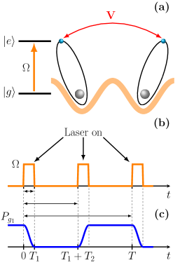
Figure 1: In (a) scheme of two interacting qubits, for instance, two-level Rydberg atoms trapped in an optical potential and experiencing a nearest-neighbour coupling $V$. They are driven by a common laser field, periodically switched on for the duration $T_{1}$ and off for the time $T_{2}$, in a sequence with temporal periodicity $T=2T_{1}+2T_{2}$ as schematized in (b). For a perfect excitation, as with $\pi$ pulses for one-photon absorption, the $P_{g}$ ground state occupation experiences the temporal evolution shown in (c).

The control of the wavefunction phase accumulation has received much attention in different contexts of quantum optics, such as the collapse and subsequent revival of atomic coherence for Bose-Einstein condensates in Mahmud and Tiesinga (2013); Meinert et al. (2014). Phase correlation destructions and revivals in the time evolution of dipole-blockaded Rydberg states have been investigated under a detuned and continuous excitation in Fan et al. (2019), and for periodic excitation by Fan et al. (2020) within the context of discrete time crystals. The quantum control of the phase accumulated by laser driving for interacting Rydberg atoms was studied in Bhaktavatsala Rao and Mølmer (2014); Beterov et al. (2020). An analysis of laser imperfections in the coherent excitation to atomic Rydberg states was experimentally investigated in de Léséleuc et al. (2018).

We introduce here the approach shown in Fig. 1(a), based on the interaction between the "computation" qubit and an additional "correction" qubit, widely used for the implementation of high fidelity quantum-nondemolition measurements Walls and Milburn (1995); Nielsen and Chuang (2000). The idea of using additional qubits for correction is taken from quantum-error-correction protocols and fault-tolerant quantum computing Nielsen and Chuang (2000), see, e.g., Egan et al. (2021) for a recent experimental realisation using ion qubits.

In the following, we use the additional phase created by the interaction to compensate for the above unwanted phase in the evolution of the computational qubit. By a proper choice of the interaction strength, we realize compensation for a long sequence of unitary operations of the computational qubit. The compensation efficiency is measured by the wavefunction fidelity reached at the end of the sequence. We obtain a high efficiency for sequence numbers up to fifty. For the long sequence of applied unitary transformations, we derive conditions for the wavefunction phase to maintain the targeted value. In most of the explored qubit level schemes, our approach leads to a magic condition for the required interaction, magic because it creates compensation for a large range of unitary transformation errors. Our approach is similar to the method of composite pulses Levitt (1986); Jones (2011). In both cases, the phase of the qubit wavefunction accumulated by the laser-pulse sequence produces a more robust qubit excitation. As main difference, the composite-pulse sequence targets a very large and stable fidelity for a single excitation. We target instead a stable and large fidelity in a long sequence of qubit operations. Our qubit interaction is linked to the excited state occupation, for instance, in experimental implementations based on atomic Rydberg excitations Saffman et al. (2010a); Labuhn et al. (2016); Adams et al. (2019); Zhang et al. (2020) or on Rydberg-dressed atomic gases Borish et al. (2020). The interaction can, in principle, be tuned experimentally. Its amplitude depends, e.g., on the atomic quantum number, and in addition, in the presence of the Förster resonances, it may be controlled by an applied electric field Ravets et al. (2014); Higgins et al. (2017); Huang et al. (2018); Beterov et al. (2020). Similar tunable interactions are present in other realisations as well, e.g., in semiconductors Schwartz et al. (2021) or in artificial atoms, as in the ground state interactions in double quantum dots in a nanowire Taherkhani et al. (2019).

The compensation scheme is applied here to a computational qubit that, under proper laser handling, experiences a Bloch sphere rotation and reinitialization within a given interrogation time interval. We repeat the same sequence on a regular basis, and introduce small errors on the laser parameters. Therefore, the qubit accumulates an unwanted phase limiting the computation utility. The compensation recovers its utility through the controlled interaction with the correction qubit. In the following, we specifically consider three situations: two models with a one-photon excitation and one with a two-photon excitation.

First we consider the one-photon excitation case. Starting from the two qubits sketched in Fig. 1, under the condition for which the laser drive does not influence the correction qubit, the impact of the interaction between the excited levels may be modelled for the computational qubit as an effective shift of the excited level. This gives our system (i): a two-level system exposed to laser pulses driving transitions between the ground and excited state. In the second configuration, the laser drive couples only to the Bell triplet states and thus the four two-qubit levels can be reduced to three simply by neglecting the Bell singlet state. This three-level system is our model (ii). There is a fundamental difference between these two models: errors in the laser drive can occur only on the computational qubit in (i), while in (ii) both qubits fully participate, with errors that can be modelled on both. The compensation works well in both cases but the magic value is more stable, producing a larger compensated area with fidelity error of the order of $10^{-6}$, for system (i). The compensation is applied to errors in the dynamics of the computational qubit on a Bloch sphere: rotation angle errors and rotation axis ones, produced by imperfections in the laser intensity and in the laser detuning, respectively. We analyze the one-photon excitation by a $\pi$ laser pulse, allowing a transition at the quantum-speed limit, but with a large sensitivity to the laser excitation parameters Giannelli and Arimondo (2014). The $\pi$ pulses are employed for both the qubit excitation and its reinitialization.

In addition to the one-photon population transfer between ground and upper states, we analyze also a two-photon excitation scheme in which the two levels of each qubit cannot directly be coupled by the laser, but are coupled through a third intermediate level. The two-photon excitation analyzed in this case is implemented via a STIRAP in cascade configuration  Vitanov et al. (2017) with temporal shifted Pump/Stokes laser pulse, providing a large and stable excitation. The application of a double-STIRAP, with inverted Pump/Stokes pulses in the second one, produces the qubit excitation and reinitialization. Similar double-STIRAP pulses are analyzed in Beterov et al. (2013) for the implementation of quantum logic gates with Rydberg atomic ensembles. In several configurations, the three-level STIRAP system may be reduced to a two-level one, where our one-photon compensation scheme may be applied. Instead, we show that the compensation even works in the non-adiabatic regime, where the two level simplification cannot be used Laine and Stenholm (1996); Vitanov and Stenholm (1996); Torosov and Vitanov (2013).

The paper is organized as follows: Sec. II describes the temporal sequence of the computation and reinitialization operations based on the two qubits, the computation and correction one. Such a sequence is repeated for a longer time period allowing the execution of repeated operations. Sec. III describes the laser driving of the qubits, the corresponding one-photon excitation models and, finally, the double-STIRAP setup for a two-photon excitation. Moreover, Sec. III introduces the fidelity as a measure of the compensation efficiency. Section IV describes the results of the compensation approach, depending on the form of the excitation, based on either single or two-photon processes. Sec. IV also presents an alternative and practically useful compensation search tool. Sec. V concludes our work.

II Qubit correction

We deal with two $j={1,2}$ qubits, the first denoted as "computational" qubit and the second one as "correction" qubit. The computational one performs a quantum computation operation and repeats its work $n$ times, with $n$ up to 50 in our simulations. Under laser driving, this qubit starts from the initial ground state $|g_{1}\rangle$ at time $t=0$, is excited to the state $|e_{1}\rangle$ to perform its operation, is reinitialized and is ready for the next round at time $t=T$. A not perfect laser driving leads, at time $T$, to computation/reinitialization errors that propagate in the operation sequence. We target to compensate for these errors.

Our correction process, schematized in Fig. 1(a), is based on the interaction of the first qubit with the correction qubit. These two qubits, supposed either equal or different, experience in their excited states $|e_{j}\rangle$ an interaction with controllable amplitude $V$ described by the following Hamiltonian in $\hbar$ units:

$$H_{V}=V|e_{1}\rangle|e_{2}\rangle\langle e_{1}|\langle e_{2}|\,.$$ (1)

By a proper choice of the interaction amplitude $V$, the phase introduced into the computational qubit will compensate for laser driving errors.
In our description, the computational process is represented by an elementary step, for instance a rotation of the Bloch vector by a $\pi$ angle Nielsen and Chuang (2000). In this simple approach also the reinitialization is based on a $\pi$ pulse. The computation/correction sequence is based on the following steps, as in Fig. 1(b). At time $t=0$, the computational qubit, initially in its ground state, is transferred to the state $|e_{1}\rangle$ by a laser pulse of time $T_{1}$. In the following time interval $T_{2}$, the interaction $V$ only determines the qubit evolution. Then an additional laser pulse of duration $T_{1}$ transfers the occupation of state $|e_{1}\rangle$ to the ground state. An interaction of duration $T_{2}$ completes the sequence with total time $T=2T_{1}+2T_{2}$. Under perfect laser driving, the occupation probability of the ground state of the computational qubit follows the time dependence in Fig. 1(c). More precisely, owing to the parity of the ground/excited states, the laser driving takes place through either a one-photon transition or a two-photon one, with a resonant or non-resonant intermediate level.

In the following, we will consider two configurations for the correction qubit in the single-photon excitation case. In the first configuration (i), denoted as two-level q-system in the following, the control or correction qubit is not exposed to the drive. Under this assumption, the effect of the second static qubit on the computational one is modelled by an effective level shift of its excited state. While in the second configuration (ii), denoted as three-level q-system, the imperfect laser excitation drives both qubits simultaneously, producing an equivalence to the Rydberg blockade. The last example we propose is the error compensation in a two interacting three-level setups both driven by the same two-photon STIRAP excitation process.

III Qubit laser handles

III.1 Single-photon excitation

For both the two- and three-level cases, the qubits interact with a laser with detuning $\delta=\omega_{L}-\omega_{0}$ from the $\omega_{0}$ ground/excited state transition and Rabi frequency $\Omega$. The $H_{0j}$ Hamiltonian of each atom $(j=1,2)$ in the rotating wave approximation (RWA) in the frame rotating with the drive, is written in units of $\hbar$ as

$$H_{0j}=-\delta|e_{j}\rangle\langle e_{j}|+\frac{\Omega}{2}\left(|g_{j}\rangle\langle e_{j}|+|e_{j}\rangle\langle g_{j}|\right).$$ (2)

The RWA, in this case, remains valid in the regime where $\Omega\ll\omega_{L}$, namely when the operation frequencies we are interested in are much smaller than the carrier frequency of the laser Shore (2011). Having in mind typical quantum-optical realizations based on Rydberg atoms this condition is usually satisfied.
The transfer to the excited states and back is produced by $\pi$-pulses with $\delta=0$, and $\Omega T_{1}=\pi$. The ground state occupation reported in Fig. 1(c) is obtained under these conditions.

III.1.1 Two-level q-system (i)

Here we suppose that the computational and the correction qubit can be addressed independently. Then we may assume that the laser excitation does not influence the correction one, e.g., due to a large difference in transition frequency of two different atoms. For instance, for Rydberg atoms in the presence of Förster resonance Ravets et al. (2014), we may suppose that the correction qubit remains in a long-lived $|e_{2}\rangle$ state, the interaction being controlled by switching on/off an electric field. The analysis of the two-level q-system (i) is a very useful step, because it is simpler since the interaction reduces here just to an effective energy shift of the computation qubit. Nevertheless this case leads to the same general compensation scheme valid also for our more complex model (ii)

III.1.2 Three-level q-system (ii)

As mentioned in the previous section, in this case the laser excitation drives both qubits simultaneously and equally. Here the Dicke states represent a convenient basis Ficek and Tanaś (2002); Comparat and Pillet (2010); Almutairi et al. (2011) for the description. Starting from the $|g_{1},g_{2}\rangle$ state at $t=0$, only the $|e_{1},e_{2}\rangle$ doubly excited state and the $|s\rangle=(|g_{1},e_{2}\rangle+|e_{1},g_{2}\rangle)/\sqrt{2}$ symmetric states (equivalent to the Bell triplet states) are occupied by the laser excitation with no occupation of the antisymmetric Bell/Dicke state (equivelent to the Bell singlet state). Therefore the wavefunction is written as

$$|\psi_{tot}\rangle=c_{gg}|g_{1},g_{2}\rangle+c_{s}|s\rangle+c_{ee}|e_{1},e_{2}\rangle\,,$$ (3)

and we effectively deal with a three-state system. The Hamiltonian for the two coupled two-level systems (qubits) and its reduction to the symmetric Dicke states is given in app. A.

Let us notice important features playing a key role in the compensation process. Both laser detunings and inter-qubit interaction are diagonal terms, see Eq. (15) in app. A. From the mathematical point of view, the evolution depends only on the sign conformity of those parameters. This feature will apply also to the compensation results. From a physical point of view the diagonal terms may be used to balance each other. This balance occurs in the Rydberg blockade Saffman et al. (2010a), where the interaction is large enough to block the laser excitation to the state $|e_{1},e_{2}\rangle$. Viceversa the tuning of those parameters has been used to enhance that excitation as in the ultracold Rydberg atom antiblockade Ates et al. (2007); Amthor et al. (2010) or in the Rydberg enhancement of a room temperature vapor Kara et al. (2018). We operate with Rabi frequencies of the laser excitation, much larger than the interaction $V$, where the above processes should not occur.

III.2 Two-photon excitation

In the previous sections, we have described the single-photon excitation in the two configurations (i) and (ii). In this section, instead, we show the laser handling for a two-photon excitation scheme. In this case, the $|g_{j}\rangle$ ground and $|e_{j}\rangle$ $(j=1,2)$ excited states, that form the qubits, in a cascade configuration are linked by two laser fields (denoted as Pump and Stokes) through the intermediate state $|i_{j}\rangle$. The Hamiltonian $H_{0j}$ representing one of the two qubits is in a frame doubly rotating at the driving frequencies and in the rotating wave approximation

$$H_{j}(t)=\ \begin{pmatrix}0&\frac{\Omega_{P}(t)}{2}&0\\ \frac{\Omega_{P}(t)}{2}&-\Delta&\frac{\Omega_{S}(t)}{2}\\ 0&\frac{\Omega_{S}(t)}{2}&-\Delta_{2}\end{pmatrix},$$ (4)

with $\Delta$ the intermediate level detuning, $\Delta_{2}$ the two-photon detuning, $\Omega_{P}$ and $\Omega_{S}$ the Pump and Stokes Rabi frequencies, respectively. For the resonant STIRAP excitation ($\Delta_{2}=0$) with temporally shifted Pump/Stokes laser pulses Vitanov et al. (2017), the Rabi frequencies have the following Gaussian shaped temporal dependencies:

$$\Omega_{P}(t)=\Omega_{0}e^{-\left(\frac{t-T_{1}/2}{T_{G}}\right)^{2}},\quad\Omega_{S}(t)=\Omega_{0}e^{-\left(\frac{t+T_{1}/2}{T_{G}}\right)^{2}},$$ (5)

with $\Omega_{0}$ peak value and width $T_{G}/\sqrt{2}$. They are parametrized such that the pulse crossing takes place at $t=0$, and the separation between two subsequent maxima is $T_{1}$. For the transfer back to the ground state with an inverted Pump/Stokes temporal dependencies, the pulse crossing occurs at time $t=T_{2}$. The time sequence of the laser driving is represented with dashed lines in Fig. 2, please see the right vertical scale for the Rabi frequencies. In order to maintain generality with respect to the experimental implementations, we work with STIRAP standard dimensionless quantities $\Omega T_{G}$ and $\Delta T_{G}$. This double-STIRAP sequence has been investigated previously, e.g., in Higgins et al. (2017); Beterov et al. (2020).

An efficient and stable STIRAP transfer is realized by imposing an adiabatic evolution of the dark state $|D_{j}\rangle$ Arimondo (1996); Fleischhauer et al. (2005) defined as

$$|D_{j}(t)\rangle=\cos\theta(t)|g_{j}\rangle-\sin\theta(t)|e_{j}\rangle,$$ (6)

with $\theta(t)$ given by $\tan\theta(t)=\Omega_{P}(t)/\Omega_{S}(t)$. If the STIRAP parameters are slowly varied, the qubit initially prepared in the ground state $|g_{j}\rangle$ follows adiabatically the instantaneous dark state, ending up in the target state $|e_{j}\rangle$ with very large fidelity. Nonadiabatic coupling between the eigenstates is negligible when the $\theta(t)$ mixing angle rate is smaller than the $\sqrt{\Delta^{2}+\Omega_{P}^{2}+\Omega_{S}^{2}}$ separation of the Hamiltonian eigenvalues Shore (2017). Robust and efficient STIRAP transfers occur at large values for both Rabi frequencies and intermediate state detuning. There, an adiabatic elimination of the intermediate state leads to an effective two-level system where our one-photon compensation may be applied. Instead, we investigate a nonadiabatic regime where the stability with respect to imperfections in the laser parameter is very limited. This occurs for low $\Delta$ values, where the fidelity presents large oscillations as a function of the laser detuning, see, e.g., Vitanov and Stenholm (1997). This is seen in Fig. 2, where the fidelity $\mathcal{F}=0.98$ at the end of the first double-STIRAP is not good enough for quantum computation purposes. The complex dependence on $\Delta$ will appear below in Fig. 8(a).

While the ground $\ket{g_{1}}$ and the excited $\ket{e_{1}}$ states of the three-level STIRAP system are described by Eq. (4) for the computation qubit, an identical copy forms the control qubit (j=2) that interacts with the first one via an interaction $V$ only between the two excited states, see Eq. (1).

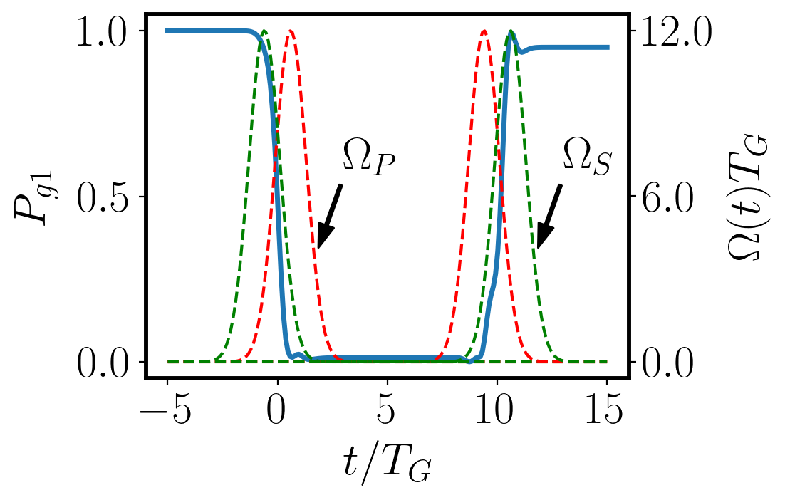
Figure 2: Evolution of the $P_{g1}$ population (blue solid line), and of the $\Omega_{p},\Omega_{S}$ Rabi frequencies (dashed lines) for a total time $T$, based on a double-STIRAP transfer sequence to the excited state and back to the ground, as for an atomic Rydberg state. Parameters $T_{G}=1$, $T_{1}=1.2$, $\Delta=\Delta_{2}=0$, $\Delta T_{G}=1.4$, $\Omega_{0}T_{G}=12$, and $T_{2}=10$. The $P_{g}$ occupation scale is on the left, and the $\Omega(t)T_{G}$ scale is on the right. The $P_{g1}$ temporal evolution over a single $T$ sequence presents the coherent oscillations discussed in Laine and Stenholm (1996).

III.3 Fidelity/Infidelity

The efficiency of the correction qubit approach will be measured at the times $t=nT$ by the fidelity $\mathcal{F}$, or the infidelity $\mathcal{I}=1-\mathcal{F}$, between the final and the initial (ground) state $|g_{1}\rangle$ of the first qubit. For the two-state q-system (i), presented in Sec. III.1.1, the straightforward fidelity is, given an arbitrary state of the first qubit $\ket{\psi_{1}}$,

$$\mathcal{F}_{1}(t=nT)=\left|\langle g_{1}|\psi_{1}(nT)\rangle\right|^{2}.$$ (7)

For the three-level setup of Sec. III.1.2, instead, the required fidelity is obtained by performing a reduction (partial trace Nielsen and Chuang (2000)) to the total density matrix. Using the $\psi_{\rm tot}$ wavefunction in the Dicke state basis of Eq. (3), the fidelity is given by

$$\mathcal{F}_{2} =\text{Tr}[(\ket{g_{1}}\bra{g_{1}}\otimes\mathbb{1}_{2})(\ket{\psi_{\rm tot}}\bra{\psi_{\rm tot}})]$$

$$=|c_{gg}(nT)|^{2}+\frac{1}{2}|c_{s}(nT)|^{2}\,.$$ (8)

This fidelity contains the predicted occupation of the computational ground state and an additional term associated to the identity of the two qubits.

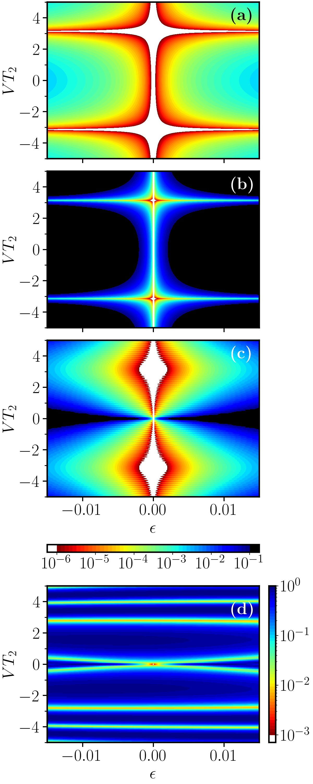
Figure 3: 2D contour plots of the logarithmic scale $\mathcal{I}$ infidelity in the ($\epsilon$, $VT_{2}$) plane for a rotation error. The colour scale below (c) applies to the plots (a-c). The black/white regions indicate infidelity values larger/smaller than the color scale limits. Plot of $\mathcal{I}_{1}(t=T)$ in (a), $\mathcal{I}_{1}(t=50T)$ in (b), and $\mathcal{I}_{2}(t=50T)$ in (c, d). In (a), and (b) the error compensation corresponds to the configuration (i) of Sec. III.1.1, in (c, d) the model (ii) of Sec. III.1.2. In (d) the interaction is continuously active.

IV Fidelity compensation

In typical applications as considered here, the Rabi frequency $\Omega$ can be much larger than the interaction $V$ between control and computational qubit. In this case, the duration $T_{1}$ of a $\pi$-pulse is much shorter than the time $T_{2}$ needed for the interaction to have a sizeable effect. In the limit $T_{1}\ll T_{2}$, it is then justified to treat $V$ as being non-zero only during the interval $T_{2}$. This assumption enables a simpler analytical treatment adopted in the following expressions, while the general configuration is addressed numerically.

We now address typical errors that lead to imperfect population transfer: in Sec. IV.1.1 an error in the rotation angle of the Bloch vector of the form $\sigma_{x}$, and in Sec. IV.1.3 of the rotational axis of the form $\sigma_{z}$.

Given, e.g., the well known long lifetime of the excited Rydberg states Saffman et al. (2010b), other effects of decoherence can be safely neglected.

IV.1 Single-photon excitation

IV.1.1 Rotation angle error

For the Rabi $\pi$ pulse applied over the $T_{1}$ time, we introduce a relative error $\epsilon$ given by

$$\Omega T_{1}=\pi(1+\epsilon)$$ (9)

associated to the Bloch vector rotation angle Nielsen and Chuang (2000).
At the time $t=T=2T_{1}+2T_{2}$, after the first sequence with two $\pi$ pulses and an acquired phase from the excited state evolution, the ground state fidelity $\mathcal{F}_{1}(t=T)$ for the two-state setup is

$$\mathcal{F}_{1}(t=T)= 1-\frac{1}{2}\sin^{2}\left(2\pi\epsilon\right)\left[1+\cos\left(VT_{2}\right)\right]$$

$$\approx 1-2(\pi\epsilon)^{2}\left[1+\cos\left(VT_{2}\right)\right],$$ (10)

in the second line at small $\epsilon$ values. The above expressions report an important feature associated to all the compensation schemes here examined. The $VT_{2}=(2m+1)\pi$ value, with $m$ integer, is "magic" because it produces a strong recovery of the fidelity for the driving error. The excited state phase shift leads to a positive interference in the wavefunction evolution at all the times $t=nT$. At the magic values, the interaction steps preceding and following the second laser pulse produce the exact reverse of the first pulse rotation angle, as shown in Appendix B. The complete qubit sequence reduces to the identity, and the initial state is exactly restored for any value of $\epsilon$. While a full recovery is obtained for all $n$ values at the magic value, Eq. (10) reports a fidelity very close to the one for interaction strengths near the magic value. This phase compensation mechanism has a strong analogy with the spin echo and dynamical decoupling techniques Viola et al. (1999); Lidar and Brun (2013), where an arbitrary phase shift is compensated by a double laser excitation. It is also analog to the anti-resonances of the quantum kicked-rotor model where each pulse exactly counteracts the preceding one due to a proper choice of free phase evolution in-between the two pulses Izrailev (1990); Sadgrove and Wimberger (2011).

With the laser acting on the computational qubit only, namely in our model (i), the plots in the $(\epsilon,VT_{2})$ plane report the resulting infidelity $\mathcal{I}_{1}(t=T)$ in Fig. 3(a) and $\mathcal{I}_{1}(t=50T)$ in (b). These plots, as most of the following ones, are limited on the horizontal to the $|\epsilon|\leq 0.015$ value, easily reached in experiments, and to $|VT_{2}|\leq 5$ owing to the vertical periodicity (phase) of the compensation. The infidelity range reported in the plots corresponds to standard quantum computation experiments. The plots highlight that the compensation scheme works very well. However, increasing the qubit cycling number, the compensation range around the magic value becomes narrow, and requires a more precise choice of the interaction parameter. The compensation efficiency appears clearly from the data of Fig. 4 where the compensated fidelity $\mathcal{F}_{1}$ vs. $n$ is compared to the fidelity reached in multiple operations in the absence of the compensation. For highlighting the robustness of the compensation, notice that the chosen parameter $V$ is only close to the magic value. Therefore, a small imperfection in the product $VT_{2}$ does not affect the efficiency of the compensation.

In the three-level q-model (ii), instead, the simultaneous driving of both the computation and compensation qubit leads to slightly different features in the time evolution, but the compensation is still produced by the combination of the in-phase laser excitation and the phase acquired here by the state $|e_{1},e_{2}\rangle$ with the laser excitation off. For $V$ off while the laser is on, an analytical solution of the Dicke state time evolution, followed by a projection on the single qubit space, produces the fidelity at time $t=T$ reported in Appendix A with a complex dependence on sine and cosine functions. At small $\epsilon$ values the fidelity, from Eqs. (16) and (17), becomes

$$\mathcal{F}_{2}(t=T)\approx 1-\frac{1}{2}(\pi\epsilon)^{2}\left[1+\cos\left(VT_{2}\right)\right].$$ (11)

Only for one rotation at time $t=T$, the phase shift $\pi$ remains magic. However, as the number $n$ of interrogations increases, the behavior of the setup (ii) is different from the case (i). The fidelity of the three-level model remains overall higher than the one of the two-level one, as can be appreciated from a comparison between the plots (b) and (c) of Fig. 3. It should be mentioned here that from the time $t=2T$ onwards the contribution of the Dicke/Bell symmetric state remains below the $10^{-5}$ level, therefore with an operating compensation, the computational qubit is in perfect shape for continuing its job.

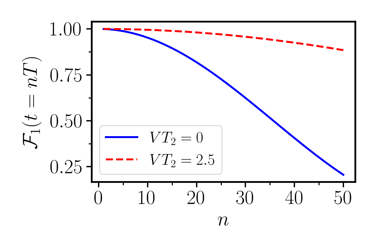
Figure 4: Fidelity $\mathcal{F}_{1}(t=nT)$ vs. the sequence number $n$ at a given error $\epsilon=0.007$: in the absence of compensation (solid blue line) and for $VT_{2}=2.5$ (red dashed line) close to the optimal compensation for a laser driving of the setup (i).

For the case when the interaction $V$ is applied also within the laser excitation period $T_{1}$, the full analytical solution is not available. Therefore we rely on numerical simulations, such as shown in Fig. 3(d), for the three-level model driving as in all the following figures. The response to the compensation is greatly modified with an optimal compensation that is almost independent of the error $\epsilon$ (for the explored range) at new magic values $VT_{2}=\pm 2.8$ and $VT_{2}=\pm 3.9$. These values converge to the previous magic ones at larger values of the ratio $T_{2}/T_{1}$.

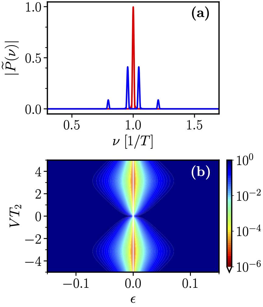
Figure 5: In (a) $|\tilde{P}(\nu)|$ Fourier spectrum of the population difference for the two-level setup (i) at $\epsilon=0.1$ and for $VT_{2}=1$. The sidebands and the splitting are well distinguishable only at these large $\epsilon$ values. They coalesce into $\nu_{0}$ for the magic compensation value, represented schematically by the red curve. In (b) we show $1-\tilde{P}(\nu_{0})$ on a logarithmic scale vs. the parameter plane $(\epsilon,VT_{2})$ for the rotation error. The white regions indicate infidelity values smaller than the minimum of the color scale.

IV.1.2 Compensation search tool

Although the study of the fidelity allows us to identify parameter values giving the desired compensation at fixed interrogation times $t=nT$, these values may not guarantee the same fidelity for different $n$. Therefore, we present now a simple approach for determining the compensation parameters guaranteeing high fidelity for all periods $nT$. It is based on the Fourier components of the population difference $P(t)=P_{g}(t)-P_{e}(t)$. At $\epsilon=0$ and at perfect compensation, $P=P_{g}-P_{e}$ is a periodic function whose Fourier spectrum contains a single component at $\nu_{0}=1/T$. At the $\epsilon\neq 0$ rotation error, a splitting into two sidebands arises in the population difference of the Fourier spectrum $\tilde{P}(\nu)$ at the frequencies $\nu_{0}(1\pm\epsilon T_{1})$, as from the two-level Rabi evolution for $\pi$ pulses. The interaction $V$ modifies the sideband positions appearing in Fig. 5(a), with a sinusoidal dependence on $VT_{2}$. It also introduces additional weaker sidebands at even larger $\epsilon$ values. At the interaction values of best compensation, the main sideband ideally coalesce into the $\nu_{0}$ value. The $1-\tilde{P}(\nu_{0})$ amplitude of the Fourier spectrum peak vs. the $(\epsilon,VT_{2})$ parameters allows a simple determination of the compensation range, as in Fig. 5(b). The analogy between this plot and that of Fig. 3(c) highligths the utility of this search tool in the full parameter space for the compensation.

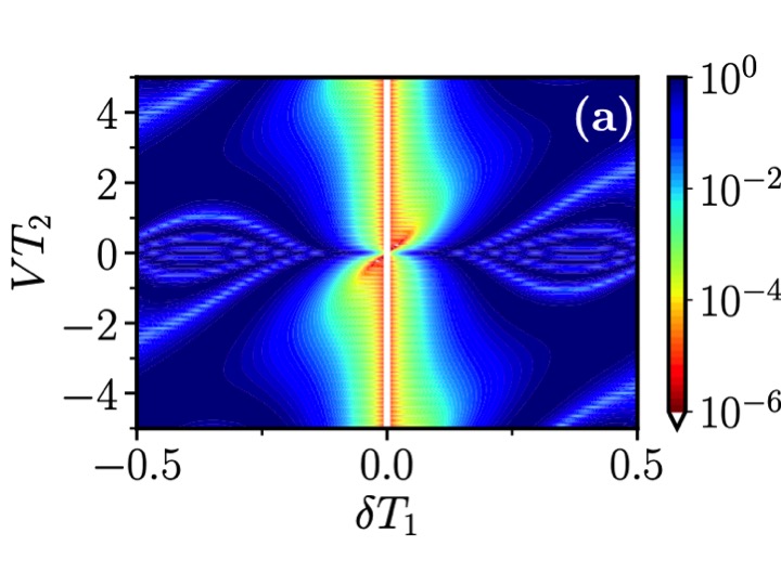
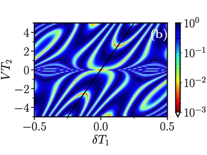
Figure 6: Two-level q-system (i): 2D plots of the $\mathcal{I}_{2}(t=50T)$ infidelity plot vs. the $(\delta T_{1},VT_{2})$ parameters for the laser detuning error. Panel (a) is obtained for the case of $V$ off in the periods when the laser is on. In (b) the interaction is on at all times. Here, the tilted black line corresponds to the Rydberg enhancement condition $V=2\delta$, see main text.

IV.1.3 Rotation axis error

We examine here the compensation of an error associated to the Bloch vector rotation axis Nielsen and Chuang (2000). We suppose that the laser detuning $\delta$ error from resonance is given by

$$\delta T_{1}=\pi\epsilon\,,$$ (12)

where $\delta T_{1}\equiv\delta\cdot T_{1}$. In a $\pi$ pulse the Bloch vector rotates by the following angle

$$\Omega_{\text{eff}}T_{1}=\left[\pi^{2}+(\delta T_{1})^{2}\right]^{1/2}\approx\pi(1+\frac{1}{2}\epsilon^{2})\,,$$ (13)

to be compared to Eq. (9) of the previous case. For small $\epsilon$ values, the fidelity at the time $T$ for the model (i) configuration is

$$\begin{split}\mathcal{F}_{1}(t=T)\approx&1-2\epsilon^{2}\left[1-\cos(VT_{2})\right]\\ &-\pi\epsilon^{3}(2T_{2}+1)\sin(VT_{2})\,.\end{split}$$ (14)

Both cosine and sine dependencies on $VT_{2}$ appear in the present fidelity. These features lead to the compensation shown in Fig. 6(a). This figure may be compared to Fig. 3(c), also for the horizontal scale owing to the detuning error definition of Eq. (12). Within the central region of low $\epsilon$ error, the magic $VT_{2}=\pi$ value does not appear clearly. The sine term of Eq. (14) leads to an asymmetric response of the $(\delta T_{1},VT_{2})$ plot, breaking the analogy with the Rabi error where a $\delta$ symmetry is valid for all the $\epsilon$ values.

The results for an interaction $V$ acting at all times are shown in Fig. 6(b). The diagonal line dependence of the top figure is greatly enhanced. For a given value of $V$, the compensation is effective within a more limited range of the detuning error. In order to obtain a wider range of error compensation, the role of $V$ within the laser interaction period is reduced by decreasing the ratio $T_{1}/T_{2}$.

The diagonal response in Fig. 6(a) for very small values of $\delta T_{1}(\approx 0.05$) and in (b) globally, is evidence of the Rydberg antiblockade/enhancement. The doubly excited state for the two atoms is reached for $\delta=V/2$, i.e., $\omega_{L}=\omega_{0}+V/2$, taking into account our definition of the interaction energy $V$ provided to the two atoms. This condition corresponds to the black line shown in Fig. 6(b). The excitation of both qubits associated to the enhancement allows for the computational qubit to acquire the phase shift required for the compensation. Notice that, owing to our choice of the laser driving parameters, $\Omega\gg V$, the Rydberg enhancement, and also the blockade, are supposed to be negligible Saffman et al. (2010a). However, even a weak enhancement may contribute essentially to the more sensitive phase-compensation.

IV.2 Double-STIRAP compensation

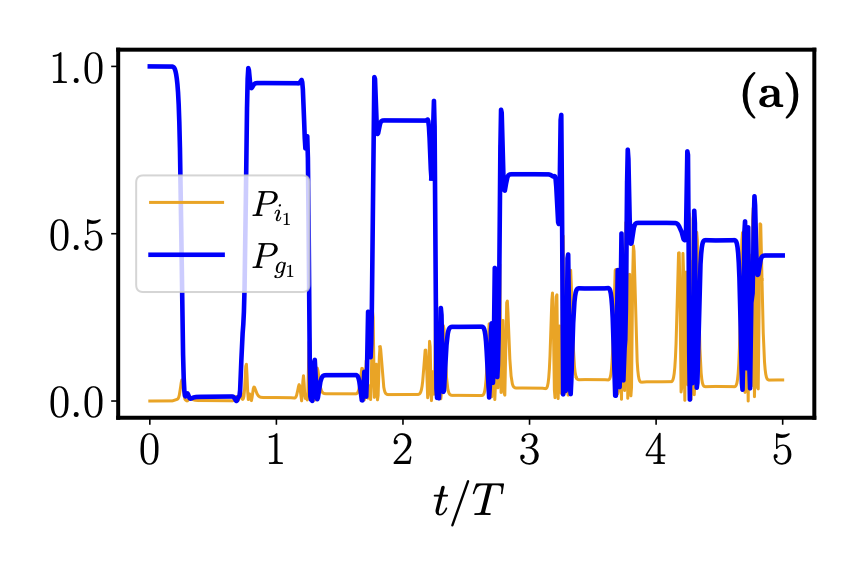
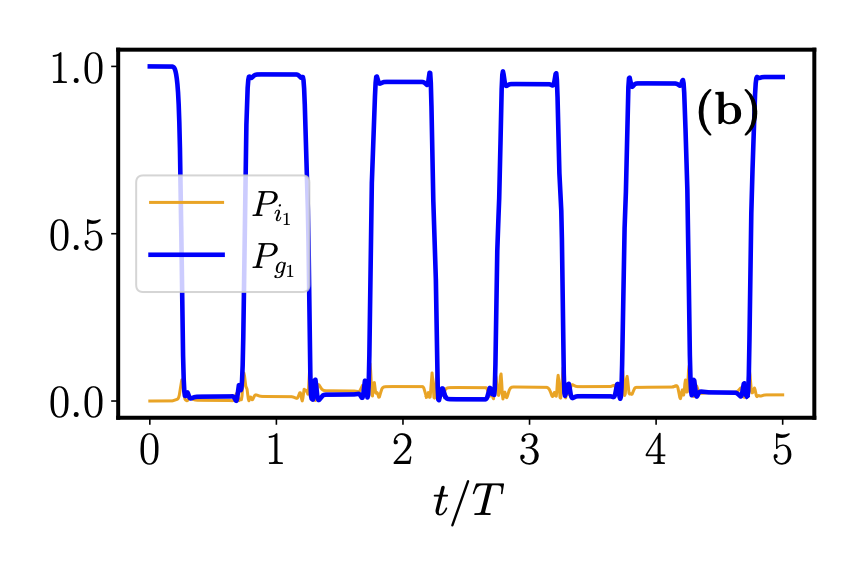
Figure 7: The $P_{g1}$ population (thick blue solid line) and $P_{i1}$ (thin orange line) vs. $t$ time up to $5T$ for a double-STIRAP operation with $\Delta T_{1}=1.4$ and parameters as in Fig. 2. (a) without compensation and (b) with an applied compensation $VT_{2}=2$. Notice the large increase in fidelity produced by the compensation, from $\mathcal{F}_{2}(t=5T,V=0)\simeq 0.43$ to $\mathcal{F}_{2}(t=5T,VT_{2}=2)\simeq 0.96$.

We now turn to the two interacting STIRAP configurations introduced in Sec. III.2. In the case of the two-photon resonant excitation $\Delta_{2}=0$, we examine the compensation for the non-adiabatic regime in which the fidelity is very sensitive to the intermediate-level detuning $\Delta$. As a consequence of the phase accumulation, such a poorly controlled response is enhanced in a long sequence of double-STIRAP pulses. The rapid decrease of the fidelity with the $n$ number, is shown in Fig. 7(a) where the $P_{g1}$ population of the initial state is plotted vs. time up to $t=5T$. Driving parameters are as in Fig. 2. An important new feature is the large $P_{i1}$ population occupation of the intermediate state, contributing to less efficient transfer processes with increasing sequence number $n$. The complex dependence of the infidelity on $\Delta$ is presented in Fig. 8(a) evidencing its drastic increase around the value $\Delta T_{1}=1.4$.

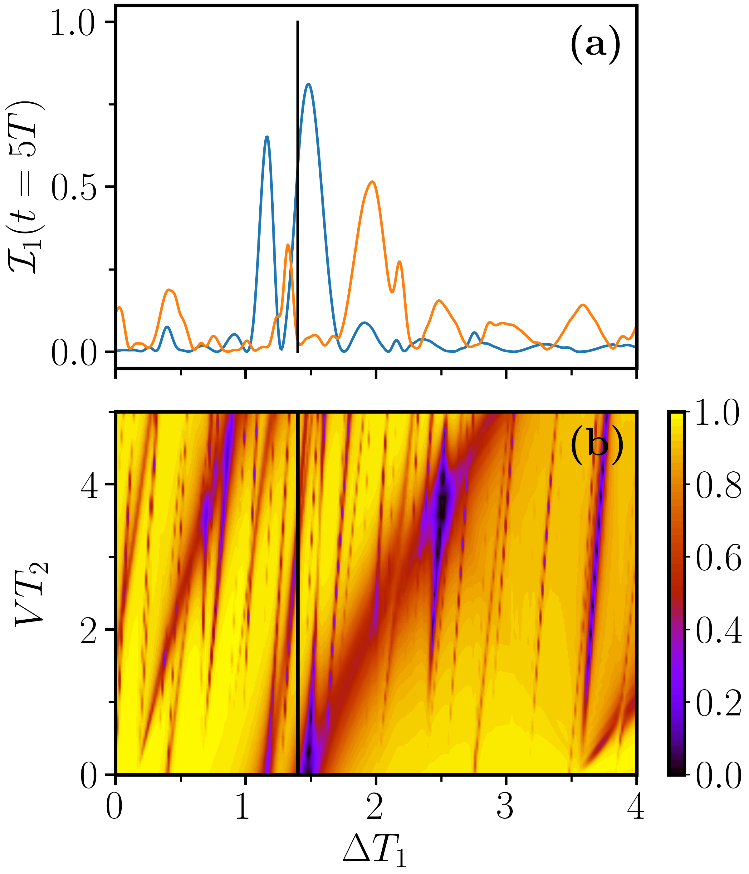
Figure 8: In (a) $n=5$ infidelities vs. the intermediate level detuning $\Delta$, blue line without compensation and symmetric with respect to the sign of $\Delta$; orange line for an applied compensation $VT_{2}=2$ and not symmetric with respect to the sign of $\Delta$. The black vertical line marks the $\Delta T_{1}=1.4$ value of Figs. 2 and  7. The other STIRAP parameters are those given in Fig. 2. (b) two-dimensional $(\Delta T_{1},VT_{2})$ plot of the $1/T$ Fourier spectrum component for the compensation search. The compensation is efficient in different regions of the parameter plane. The black vertical line identifies the $\Delta T_{1}=1.4$ value, as in (a).

We analyze the Fourier spectrum to determine the compensation values when the interaction $V$ is applied at all times. As an example, Fig. 7(b) shows the good and stable fidelity of the computational qubit up $n=5$ when an interaction compensation $VT_{2}=2$ is applied for the laser parameters of the figure. Very similar results are obtained if the interaction is switched on only for the $T_{2}$ periods. The two-dimensional plot in Fig. 8(b) for the central Fourier component vs. the $(\Delta T_{1},VT_{2})$ parameters, shows the presence of regions where the compensation is very efficient. The compensation remains efficient for a reasonable large range of interaction amplitudes. However, for a maximal compensation, a tuning of the interaction amplitude with the detuning value is required. It should be pointed out that the best compensation is obtained for a sign conformity between $\Delta$ and $V$, as for the data of Fig. 6. This response suggests a hidden role of the Rydberg enhancement, in appearance not connected to the $(\delta,V)$ relation discussed above for the one-photon case. In Fig. 8(b) the tilted parallel lines corresponding to constant compensation reflect the sinusoidal dependence on the parameter $VT_{2}$ appearing in the expressions for the fidelity reported above.

V Conclusions

We have introduced a model for robust quantum control, in which driving errors affecting a computational qubit are corrected or compensated via the interaction with an additional correction qubit. For the qubit Bloch vector, the standard errors on rotation angle and axis have been considered. Compensation schemes allowing a very efficient recovery of the fidelity are determined. The fidelity remains very high for up to our choice of fifty qubit operations for the parameters investigated here, but longer sequences could be explored on equal footing. An optimal control approach may be used to determine the compensation in the simultaneous presence of both rotation angle and axis errors. For ultracold atomic qubits, the interaction is naturally provided by the Rydberg interactions that represent a very efficient tool for quantum simulations or quantum computation Saffman et al. (2010b); Jaksch et al. (2000). Using the Förster resonances, the interaction amplitude is easily controlled also with a fast temporal response. For most of the explored schemes we have demonstrated that the compensation is not very sensitive to the precise value of the interaction strength or, equivalently, the interaction time $T_{2}$. In addition the required corrections are within range typically accessible in experimental realizations, and might help to improve substantially the fidelities reached in novel setups such as based on optomechanics Fedoseev et al. (2021).

The quantum control of a long sequence of qubit operations is determined by numerical calculations. However, the examination of the $t=T$ single sequence by analytical calculation, leads to compensation requirements with a precision good enough for exploring longer temporal sequences. Because the compensation efficiency becomes more critical at larger sequence numbers, it should be tuned performing numerical tests.

Our scheme has some analogy with the fidelity increase obtained in quantum gates via Rydberg interactions by driving simultaneously the control and target qubits as examined in Beterov et al. (2013); Saffman et al. (2020). It will be interesting to explore the application of our compensation to quantum gates Bhaktavatsala Rao and Mølmer (2014); Wu et al. (2021); Zhang et al. (2020). The scheme could also be extended to more elaborated STIRAP protocols, as that recently introduced in Di Stefano et al. (2016) for artificial atoms. An additional feature to be investigated is the role of qubit dissipation within the times of our compensation, in particular in view of solid-state, e.g., superconducting qubit implementations Blais et al. (2021).

VI Acknowledgments

One of the authors (E.A.) thanks G. La Rocca and D. Rossini for inspiring discussions. Special thanks goes to G. Falci for a critical reading of the manuscript.

Appendices

Appendix A Three-level q-system Hamitonian and fidelity

The aim of this Appendix is to derive the Hamiltonian for the three-level q-system, once again for the case where the interaction acts only within the $T_{2}$ periods. The solution in the Dicke basis leads to the fidelity of the computational qubit.

Within the single-qubit basis the Hamiltonian is given by the sum of $H_{01}\otimes I+I\otimes H_{02}$, with $I$ the identity matrix and $H_{0j}$ from Eq. (2), and of the interaction term of Eq. (1). As in Sec. II, the convenient basis to study the present evolution of two qubits is composed by the three symmetric Dicke states of Eq. (3). Within that basis the Hamiltonian is described by the following matrices

$$H_{0}=\begin{pmatrix}0&\frac{\Omega}{\sqrt{2}}&0\\ \frac{\Omega}{\sqrt{2}}&\delta&\frac{\Omega}{\sqrt{2}}\\ 0&\frac{\Omega}{\sqrt{2}}&2\delta\\ \end{pmatrix}, H_{V}=\begin{pmatrix}0&0&0\\ 0&0&0\\ 0&0&V\\ \end{pmatrix}\,,$$ (15)

for the laser-on periods and interaction-only periods, respectively. Notice the cooperative $\sqrt{2}$ increase of the Rabi frequency for laser excitation to the symmetric state $|s\rangle$ with respect to Eqs. (2) and (4). For $\delta=0$, the evolution equations are equivalent to the Bloch equations for a spin-1 system in resonance with the driving field. The interaction produces a $VT_{2}$ phase shift of the $|e_{1},e_{2}\rangle$ doubly excited state.

For the calculation of fidelity from Eq. (8) the following Dicke state occupations are required:

$$\begin{split}|c_{gg}(T)|^{2}=&\frac{1}{4}\Big{[}\left(1-\cos(2\Omega T_{1})\right)-\frac{1}{2}\left(1-\cos(\Omega T_{1})\right)^{2}\times\\ &\times\left(1-\cos(VT_{2})\right)\Big{]}^{2}+\\ &+\frac{1}{16}\left[1-\cos(\Omega T_{1})\right]^{4}\sin^{2}(VT_{2})\end{split}$$ (16)

$$\begin{split}|c_{s}(T)|^{2}=&\frac{1}{4}\sin^{2}(\Omega T_{1})\Big{[}\cos^{2}(\Omega T_{1})\left(5+3\cos(VT_{2})\right)+\\ &+\left(2\cos(\Omega T_{1})+1\right)\left(1-\cos(VT_{2})\right)\Big{]}\,.\end{split}$$ (17)

Using Eq. (8) the fidelity at time $(t=T)$ is obtained as

$$\mathcal{F}_{2}(t=T)=|c_{gg}(T)|^{2}+\frac{1}{2}|c_{s}(T)|^{2}\,.$$ (18)

Iterating such a procedure, one can obtain analytical expressions of the fidelity at periods $n>1$. However, due to its growing complexity, a software such as Mathematica is helpful for obtaining the rather lengthy algebraic expressions with increasing $n$. In the Delvecchio (2021) we report the Mathematica notebook for the study of the reduced three-level q-system showed in sec III.1.2.

Appendix B Two-level q-system with $VT_{2}=\pi$

The present target is to derive the magic compensation value from the temporal evolution of the two-level q-system, with time separated actions of laser and interaction. For the case of rotation angle error with an arbitrary Rabi frequency $\Omega$ including the $\epsilon$ error as from Eq. (9), the evolution operator at time $T=2T_{1}+2T_{2}$ is

$$U(T)=e^{-iVT_{2}\ket{e_{1}}\bra{e_{1}}}e^{-i\frac{\Omega T_{1}}{2}\sigma_{x1}}e^{-iVT_{2}\ket{e_{1}}\bra{e_{1}}}e^{-i\frac{\Omega T_{1}}{2}\sigma_{x1}}$$ (19)

with $\sigma_{x1}$ the Pauli matrix for the computational qubit. We demonstrate that for $VT_{2}=\pi$ the operator $U(T)$ corresponds to the identity matrix, for all the $\Omega$ values.

Let us consider the first three exponentials in Eq. (19) r.h.s.. Written in matrix form, they explicitly read

$$\begin{split}\begin{pmatrix}e^{-iVT_{2}}&0\\ 0&1\end{pmatrix}&\begin{pmatrix}\cos(\frac{\pi}{2}(1+\epsilon))&&-i\sin(\frac{\pi}{2}(1+\epsilon))\\ -i\sin(\frac{\pi}{2}(1+\epsilon))&&\cos(\frac{\pi}{2}(1+\epsilon))\end{pmatrix}\times\\ \times&\begin{pmatrix}e^{-iVT_{2}}&0\\ 0&1\end{pmatrix}\,,\end{split}$$ (20)

Setting $VT_{2}=\pi$ and performing the matrix product, we obtain

$$\begin{pmatrix}\cos(\frac{\pi}{2}(1+\epsilon))&&i\sin(\frac{\pi}{2}(1+\epsilon))\\ i\sin(\frac{\pi}{2}(1+\epsilon))&&\cos(\frac{\pi}{2}(1+\epsilon))\end{pmatrix}=e^{i\frac{\Omega T_{1}}{2}\sigma_{x}}\,.$$ (21)

This operator performs a rotation of the Bloch vectors equal and opposite to that induced by the first pulse of the sequence in Eq. (19). Inserting the latter result in that equation we obtain

$$U(T)=e^{i\frac{\Omega T_{1}}{2}\sigma_{x}}e^{-i\frac{\Omega T_{1}}{2}\sigma_{x}}=I\,,$$ (22)

demonstrating the magic value compensation, independent of the $\epsilon$ rotation angle error.

The application of the evolution operator to the case of the rotation axis error unfortunately does not produce a similar simple interpretation since both errors cannot be exactly corrected by the same procedure from above. One may apply, however, an optimal control approach to find the optimal value for the best simultaneous compensation of both errors.

References

- Nielsen and Chuang (2000) M. A. Nielsen and I. L. Chuang, Quantum Computation and Quantum Information (Cambridge University Press, 2000).
- Terhal (2015) B. M. Terhal, Quantum error correction for quantum memories, Rev. Mod. Phys. 87, 307 (2015), arXiv:1302.3428v7.
- Chiesa et al. (2020) A. Chiesa, E. Macaluso, F. Petiziol, S. Wimberger, P. Santini, and S. Carretta, Molecular nanomagnets as qubits with embedded quantum-error correction, J. Phys. Chem. Lett. 11, 8610 (2020), pMID: 32936660.
- Levitt (1986) M. H. Levitt, Composite pulses, Progr. Nucl. Magn. Res. Spectrosc. 18, 61 (1986).
- Jones (2011) J. A. Jones, Quantum computing with NMR, Progr. Nucl. Magn. Res. Spectrosc. 59, 91 (2011), arXiv:1011.1382v1.
- Guéry-Odelin et al. (2019) D. Guéry-Odelin, A. Ruschhaupt, A. Kiely, E. Torrontegui, S. Martínez-Garaot, and J. G. Muga, Shortcuts to adiabaticity: Concepts, methods, and applications, Rev. Mod. Phys. 91, 045001 (2019), arXiv:1904.08448v2.
- Glaser et al. (2015) S. J. Glaser, U. Boscain, T. Calarco, C. P. Koch, W. Köckenberger, R. Kosloff, I. Kuprov, B. Luy, S. Schirmer, T. Schulte-Herbrüggen, D. Sugny, and F. K. Wilhelm, Training Schrödinger´s cat: quantum optimal control - strategic report on current status, visions and goals for research in europe, Eur. Phys. J. D 69, 279 (2015), arXiv:1508.00442v1.
- Mahmud and Tiesinga (2013) K. W. Mahmud and E. Tiesinga, Dynamics of spin-1 bosons in an optical lattice: Spin mixing, quantum-phase-revival spectroscopy, and effective three-body interactions, Phys. Rev. A 88, 023602 (2013), arXiv:1304.7565v1.
- Meinert et al. (2014) F. Meinert, M. J. Mark, E. Kirilov, K. Lauber, P. Weinmann, M. Gröbner, and H.-C. Nägerl, Interaction-Induced Quantum Phase Revivals and Evidence for the Transition to the Quantum Chaotic Regime in 1D Atomic Bloch Oscillations, Phys. Rev. Lett. 112, 193003 (2014), arXiv:1309.4045v2.
- Fan et al. (2019) C.-H. Fan, H.-X. Zhang, and J.-H. Wu, In-phase and antiphase dynamics of rydberg atoms with distinguishable resonances, Phys. Rev. A 99, 033813 (2019).
- Fan et al. (2020) C.-H. Fan, D. Rossini, H.-X. Zhang, J.-H. Wu, M. Artoni, and G. C. La Rocca, Discrete time crystal in a finite chain of Rydberg atoms without disorder, Phys. Rev. A 101, 013417 (2020), arXiv:1907.03446v2.
- Bhaktavatsala Rao and Mølmer (2014) D. D. Bhaktavatsala Rao and K. Mølmer, Robust Rydberg-interaction gates with adiabatic passage, Phys. Rev. A 89, 030301 (2014), arXiv:1311.5147v1.
- Beterov et al. (2020) I. I. Beterov, D. B. Tretyakov, V. M. Entin, E. A. Yakshina, I. I. Ryabtsev, M. Saffman, and S. Bergamini, Application of adiabatic passage in Rydberg atomic ensembles for quantum information processing, J. Phys. B: At. Mol. Opt. Phys. 53, 182001 (2020), arXiv:2001.06352v1.
- de Léséleuc et al. (2018) S. de Léséleuc, D. Barredo, V. Lienhard, A. Browaeys, and T. Lahaye, Analysis of imperfections in the coherent optical excitation of single atoms to Rydberg states, Phys. Rev. A 97, 053803 (2018), arXiv:1802.10424v1.
- Walls and Milburn (1995) D. F. Walls and G. J. Milburn, Quantum optics / D.F. Walls, G.J. Milburn, springer study ed. ed. (Springer-Verlag Berlin ; New York, 1995) pp. xii, 351 p. :.
- Egan et al. (2021) L. Egan, D. M. Debroy, C. Noel, A. Risinger, D. Zhu, D. Biswas, M. Newman, M. Li, K. R. Brown, M. Cetina, and C. Monroe, Fault-tolerant control of an error-corrected qubit, Nature 598, 281 (2021).
- Saffman et al. (2010a) M. Saffman, T. G. Walker, and K. Mølmer, Quantum information with Rydberg atoms, Rev. Mod. Phys. 82, 2313 (2010a), arXiv:0909.4777v3.
- Labuhn et al. (2016) H. Labuhn, D. Barredo, S. Ravets, S. de Léséleuc, T. Macrì, T. Lahaye, and A. Browaeys, Tunable two-dimensional arrays of single Rydberg atoms for realizing quantum ising models, Nature 534, 10.1038/nature18274 (2016), arXiv:1509.04543v3.
- Adams et al. (2019) C. S. Adams, J. D. Pritchard, and J. P. Shaffer, Rydberg atom quantum technologies, J. Phys. B: At. Mol. Opt. Phys. 53, 012002 (2019), arXiv:1907.09231.
- Zhang et al. (2020) C. Zhang, F. Pokorny, W. Li, G. Higgins, A. Pöschl, I. Lesanovsky, and M. Hennrich, Submicrosecond entangling gate between trapped ions via Rydberg interaction, Nature 580, 345 (2020), arXiv:1908.11284v1.
- Borish et al. (2020) V. Borish, O. Marković, J. A. Hines, S. V. Rajagopal, and M. Schleier-Smith, Transverse-field Ising dynamics in a Rydberg-dressed atomic gas, Phys. Rev. Lett. 124, 063601 (2020), arXiv:1910.13687v3.
- Ravets et al. (2014) S. Ravets, H. Labuhn, D. Barredo, L. Béguin, T. Lahaye, and A. Browaeys, Coherent dipole-dipole coupling between two single Rydberg atoms at an electrically-tuned Förster resonance, Nature Physics 10, 914 (2014), arXiv:1405.7804v1.
- Higgins et al. (2017) G. Higgins, F. Pokorny, C. Zhang, Q. Bodart, and M. Hennrich, Coherent control of a single trapped rydberg ion, Phys. Rev. Lett. 119, 220501 (2017), arXiv:1708.06387.
- Huang et al. (2018) X.-R. Huang, Z.-X. Ding, C.-S. Hu, L.-T. Shen, W. Li, H. Wu, and S.-B. Zheng, Robust Rydberg gate via Landau-Zener control of Förster resonance, Phys. Rev. A 98, 052324 (2018), arXiv:1806.09775v4.
- Schwartz et al. (2021) I. Schwartz, Y. Shimazaki, C. Kuhlenkamp, K. Watanabe, T. Taniguchi, M. Kroner, and A. Imamoglu, Electrically tunable feshbach resonances in twisted bilayer semiconductors, Science 374, 336 (2021), https://www.science.org/doi/pdf/10.1126/science.abj3831 .
- Taherkhani et al. (2019) M. Taherkhani, M. Willatzen, E. V. Denning, I. E. Protsenko, and N. Gregersen, High-fidelity optical quantum gates based on type-ii double quantum dots in a nanowire, Phys. Rev. B 99, 165305 (2019).
- Giannelli and Arimondo (2014) L. Giannelli and E. Arimondo, Three-level superadiabatic quantum driving, Phys. Rev. A 89, 033419 (2014), arXiv:1402.1299v1.
- Vitanov et al. (2017) N. V. Vitanov, A. A. Rangelov, B. W. Shore, and K. Bergmann, Stimulated Raman adiabatic passage in physics, chemistry, and beyond, Rev. Mod. Phys. 89, 015006 (2017), arXiv:1605.00224v2.
- Beterov et al. (2013) I. I. Beterov, M. Saffman, E. A. Yakshina, V. P. Zhukov, D. B. Tretyakov, V. M. Entin, I. I. Ryabtsev, C. W. Mansell, C. MacCormick, S. Bergamini, and M. P. Fedoruk, Quantum gates in mesoscopic atomic ensembles based on adiabatic passage and Rydberg blockade, Phys. Rev. A 88, 010303 (2013), arXiv:1212.1138v3.
- Laine and Stenholm (1996) T. A. Laine and S. Stenholm, Adiabatic processes in three-level systems, Phys. Rev. A 53, 2501 (1996).
- Vitanov and Stenholm (1996) N. V. Vitanov and S. Stenholm, Non-adiabatic effects in population transfer in three-level systems, Opt. Comm. 127, 215 (1996).
- Torosov and Vitanov (2013) B. T. Torosov and N. V. Vitanov, Composite stimulated Raman adiabatic passage, Phys. Rev. A 87, 043418 (2013), arXiv:1306.0699v1.
- Shore (2011) B. Shore, Manipulating quantum structures using laser pulses (Cambridge University Press, 2011).
- Ficek and Tanaś (2002) Z. Ficek and R. Tanaś, Entangled states and collective nonclassical effects in two-atom systems, Phys. Rep. 372, 369 (2002), arXiv:quant-ph/0302082v1.
- Comparat and Pillet (2010) D. Comparat and P. Pillet, Dipole blockade in a cold Rydberg atomic sample, J. Opt. Soc. Am. B 27, A208 (2010), arXiv:1006.0742v1.
- Almutairi et al. (2011) K. Almutairi, R. Tanaś, and Z. Ficek, Generating two-photon entangled states in a driven two-atom system, Phys. Rev. A 84, 013831 (2011).
- Ates et al. (2007) C. Ates, T. Pohl, T. Pattard, and J. M. Rost, Antiblockade in Rydberg excitation of an ultracold lattice gas, Phys. Rev. Lett. 98, 023002 (2007), arXiv:physics/0605111v1.
- Amthor et al. (2010) T. Amthor, C. Giese, C. S. Hofmann, and M. Weidemüller, Evidence of antiblockade in an ultracold Rydberg gas, Phys. Rev. Lett. 104, 013001 (2010), arXiv:0909.0837.
- Kara et al. (2018) D. Kara, A. Bhowmick, and A. K. Mohapatra, Rydberg interaction induced enhanced excitation in thermal atomic vapor, Scientific Reports 8, 3236 (2018), arXiv:1710.05573v1.
- Arimondo (1996) E. Arimondo, Coherent population trapping in laser spectroscopy (Elsevier, 1996) pp. 257–354.
- Fleischhauer et al. (2005) M. Fleischhauer, A. Imamoglu, and J. P. Marangos, Electromagnetically induced transparency: Optics in coherent media, Rev. Mod. Phys. 77, 633 (2005).
- Shore (2017) B. W. Shore, Picturing stimulated Raman adiabatic passage: a STIRAP tutorial, Adv. Opt. Phot. 9, 563 (2017).
- Vitanov and Stenholm (1997) N. V. Vitanov and S. Stenholm, Properties of stimulated Raman adiabatic passage with intermediate-level detuning, Opt. Comm. 135, 394 (1997).
- Saffman et al. (2010b) M. Saffman, T. G. Walker, and K. Mølmer, Quantum information with rydberg atoms, Rev. Mod. Phys. 82, 2313 (2010b).
- Viola et al. (1999) L. Viola, E. Knill, and S. Lloyd, Dynamical decoupling of open quantum systems, Phys. Rev. Lett. 82, 2417 (1999), arXiv:quant-ph/9809071v2.
- Lidar and Brun (2013) D. A. Lidar and T. A. Brun, Quantum Error Correction (Cambridge University Press, 2013).
- Izrailev (1990) F. M. Izrailev, Simple models of quantum chaos: Spectrum and eigenfunctions, Phys. Rep. 196, 299 (1990).
- Sadgrove and Wimberger (2011) M. Sadgrove and S. Wimberger, Chapter 7 - A Pseudoclassical Method for the Atom-Optics Kicked Rotor: from Theory to Experiment and Back (Academic Press, 2011) pp. 315–369.
- Jaksch et al. (2000) D. Jaksch, J. I. Cirac, P. Zoller, S. L. Rolston, R. Côté, and M. D. Lukin, Fast quantum gates for neutral atoms, Phys. Rev. Lett. 85, 2208 (2000).
- Fedoseev et al. (2021) V. Fedoseev, F. Luna, I. Hedgepeth, W. Löffler, and D. Bouwmeester, Stimulated Raman Adiabatic Passage in Optomechanics, Phys. Rev. Lett. 126, 113601 (2021), arXiv:1911.11464v2.
- Saffman et al. (2020) M. Saffman, I. I. Beterov, A. Dalal, E. J. Páez, and B. C. Sanders, Symmetric Rydberg controlled- gates with adiabatic pulses, Phys. Rev. A 101, 062309 (2020), arXiv:1912.02977v3.
- Wu et al. (2021) J.-L. Wu, Y. Wang, J.-X. Han, S.-L. Su, Y. Xia, Y. Jiang, and J. Song, Resilient quantum gates on periodically driven Rydberg atoms, Phys. Rev. A 103, 012601 (2021), arXiv:2101.02328v1.
- Di Stefano et al. (2016) P. G. Di Stefano, E. Paladino, T. J. Pope, and G. Falci, Coherent manipulation of noise-protected superconducting artificial atoms in the lambda scheme, Phys. Rev. A 93, 051801 (2016), arXiv:1509.05562v2.
- Blais et al. (2021) A. Blais, A. L. Grimsmo, S. M. Girvin, and A. Wallraff, Circuit quantum electrodynamics, Rev. Mod. Phys. 93, 025005 (2021).
- Delvecchio (2021) M. Delvecchio, Two periodically driven interacting qubits (2021), mathematica notebook, available online: https://notebookarchive.org/2021-06-bjbq4hz.