CrysXPP: An Explainable Property Predictor for Crystalline Materials

Abstract

We present a deep-learning framework, CrysXPP, to allow rapid and accurate prediction of electronic, magnetic, and elastic properties of a wide range of materials. CrysXPP lowers the need for large property tagged datasets by intelligently designing an autoencoder, CrysAE. The important structural and chemical properties captured by CrysAE from the large amount of available crystal graphs data helped in achieving low prediction errors. Moreover, we design a feature selector that provides interpretability to the results obtained. Most notably, when given a small amount of experimental data, CrysXPP is consistently able to outperform conventional DFT. A detailed ablation study establishes the importance of different design steps. We release the large pre-trained model CrysAE. We believe by fine-tuning the model with a small amount of property-tagged data, researchers can achieve superior performance on various applications with a restricted data source.

1 Introduction

In recent times several machine learning techniques  [1, 2, 3, 4, 5, 6, 7, 8] have been proposed to enable fast and accurate prediction of different properties for crystalline materials, thus facilitating rapid screening of large material search spaces [9, 10, 11]. The existing techniques either use handcrafted feature based descriptors  [1, 2, 3, 4, 5] or deep graph neural network (GNN)  [6, 7, 8, 12, 13, 14, 15, 16, 17] to generate a representation from the 3d conformation of crystal structures. Generating handcrafted features requires specific domain knowledge and human intervention, which make the methods inherently restricted. Deep learning methods, on the other hand, do not depend on careful feature curation and can automatically learn the structure-property relationships of materials; thus making it an attractive candidate.
Graph neural network based approaches are getting popular recently for their ability to encode graph information in an enriched representation space. Orbital-based GNNs [16][17] use symmetry adapted atomic orbital features to predict different molecular properties. Though orbital-based GNNs predict molecular properties well, they are not an excellent choice for capturing complicated periodic structures such as crystals since they describe the nature of the electron distribution particularly close to atoms. On the other hand, motif-centric GNNs [14] [15] convert motif sub-structures of a crystal as a node and encode their inter connections for a large set of crystalline compounds using an unsupervised learning algorithm. Though they show improvements on property prediction tasks for metal oxides, their applicability is restricted as they ignore the atomic configuration inside the motif substructure which is also very important.
On a different departure, CGCNN [6], MTCGCNN [7] build a convolution neural network directly on a 2d crystal graph derived from 3d crystal structure. GATGNN [12] incorporates the idea of graph attention network on crystal graphs to learn the importance of different bonds between the atoms whereas MEGNet [8] introduces global state attributes for quantitative structure-state property relationship prediction in materials. As this class of methods aims to capture the information of any crystal graph just from the connectivity and atomic features, we contribute in this promising direction.
Like any large deep neural network based models, GNN based architectures also introduce large number of trainable parameters. Hence, to estimate these parameters correctly for better accuracy, a huge amount of tagged training data is required which is not always available for all the crystal properties. Hence developing a deep learning based model which can be trained on a small amount of tagged data would be extremely useful to infer varied properties of crystal materials. Also as available experimental data for the various properties are small and less diverse [18, 19, 20], these models are trained using data gathered from the DFT calculations [21, 22, 23]. As DFT data often differ from experimental ground truth due to its inefficiency in describing the many-body ground state, especially for properties such as band gap [24] or treatment of van der Waals interactions [25], training with DFT only method may incorporate the inaccuracies of DFT in the prediction. Moreover, in most of the cases, the existing property predictors are trained to predict a specific property. Hence, the generated descriptor or embeddings of any crystal are specific to a given property. It prevents them from sharing common structural information relevant to multiple properties. Though multi-task learning setup achieves information sharing across properties [7], it works well only for properties that are correlated with each other. Last but not least, the existing neural network based methods [9, 26, 10, 27, 7, 6, 12, 8, 13, 14, 15, 16, 17] hardly provide any explanation for their results. The lack of interpretability and algorithmic transparency allows little use of them in the field of material science. Therefore it is necessary to explore and provide the reasons behind a prediction for any give property.
In this paper, we propose an explainable deep property predictor  CrysXPP. It is built upon CrysAE, an auto-encoder based architecture that is trained with a large amount of easily available crystal data, that is, property agnostic structural information of the crystal graph. This leads to the deep encoding module capturing all the important structural and basic chemical information of the constituent atoms (nodes) of the crystal graph. The learned information is leveraged to build the property predictor, CrysXPP, where the knowledgeable encoder helps to produce high quality representation of a candidate crystal. Consequently, the property predictor provides superior performance (better than all the competing baselines) even when trained with a small amount of property-tagged data, thus largely mitigating the need for having a huge amount of dataset tagged with a specific property. The structural information learned in the encoding model of an auto-encoder is robust and can remove the error bias introduced by DFT by fine tuning the system with a small amount of experimental data, whenever available. Further, we introduce a feature selector that helps to provide an explanation by highlighting the subset of the atomic features responsible for manifestation of a chemical property of the given crystal.
Through extensive analysis of inorganic crystal data set across seven properties, we show that our method can achieve the lowest error compared to other alternative baselines; the improvement is particularly significant when only a small amount of tagged data is available for training. We have further shown that CrysXPP is effective towards removing error bias due to DFT tagged data by incorporating a small amount of experimental data in the training set for both formation energy and band gap. Finally, with appropriate case studies, we show that the feature selection module can effectively provide explanations of the importance of different features towards prediction, which are in sync with the domain knowledge.

2 Results and Discussions

2.1 Model Architecture

In this section we discuss in more detail the key technical contributions towards this goal followed by the training process and implementation details.

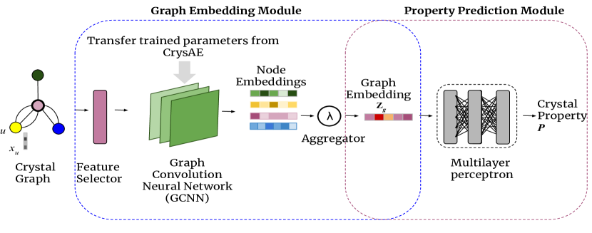
Figure 1: The architecture of Crystal eXplainable Property Predictor (CrysXPP), comprises two building blocks (a). a multilayer graph convolution neural network (GCNN) as a graph embedding module and (b). a multilayer perceptron as property prediction module. Given graph structure and node feature information, graph embedding module produces an embedding corresponding to each graph. Property predictor is a deep regressor module, which takes graph embedding as input and predicts the property value.

Overview. We propose Crystal eXplainable Property Predictor (CrysXPP), which realizes a crystalline material as a graph structure (say $\mathcal{G}$) and predicts the value of a property (eg. formation energy) given the crystal graph structure. As depicted in Fig.1, CrysXPP comprises two building blocks (a). a property prediction module and (b). a graph embedding module. In the graph embedding module we have a crystal graph encoder based on graph convolution neural network (GCNN) [6], which takes a crystal graph structure along with node and edge feature information as input and returns an embedding corresponding to each node as output. The weights of the node features (check Table 1) are determined by a feature selector layer. We consider nine different atomic properties (Table 1) as node features and the weights of those node features are determined by the feature selector layer. Moreover, the graph embedding module needs to capture the structural and chemical properties of the underlying crystal, hence one can use the huge amount of available crystal information (irrespective of the property) to train the graph convolution network. For this at first we separately train the GCNN as a part (the encoder) of CrysAE (Fig.2); and the weights thereby obtained are used as an initialization of the GCNN of CrysXPP. The structural information learned in the encoding model of CrysAE and duly transferred to the GCNN of CrysXPP makes CrysXPP more robust.
Our overall model architecture is essentially composed of the following two modules:

• Auto encoder (CrysAE):
  $q_{\bm{\theta}}:(\bm{\mathcal{V}},\bm{\mathcal{E}},\bm{\mathcal{X}},\bm{\mathcal{F}})\to\bm{\mathcal{Z}}$; $p_{\bm{\phi}}:\bm{\mathcal{Z}}\to(\bm{\mathcal{V}},\bm{\mathcal{E}},\bm{\mathcal{X}},\bm{\mathcal{F}})$

• Property predictor (CrysXPP):
  $p_{\bm{\zeta},\bm{\theta^{\prime}},\bm{\psi}}:\bm{\mathcal{X}}\to_{\bm{\zeta}}\bm{\mathcal{X}}^{\prime};(\bm{\mathcal{V}},\bm{\mathcal{E}},\bm{\mathcal{X}}^{\prime},\bm{\mathcal{F}})\to_{\bm{\theta^{\prime}}}\bm{\mathcal{Z}};\bm{\mathcal{Z}}\to_{\bm{\psi}}\mathcal{P}$

In the above characterization, $\bm{\theta},\bm{\phi},\bm{\zeta},\bm{\theta}^{\prime}$ and $\bm{\psi}$ are the trainable parameters of the respective modules. Here $\bm{\theta}$ and $\bm{\phi}$ are the parameters for the encoder and decoder respectively of the CrysAE. $\bm{\zeta}$ is the trainable parameter of feature selector ${\mathcal{S}}$, $\bm{\theta}^{\prime}$ is the parameter of the encoder and $\bm{\psi}$ is the parameter of the multi layer perceptron of CrysXPP model. We initialize $\bm{\theta}^{\prime}:=\bm{\theta}$ i.e, we first train the autoencoder and then the parameters of the encoder of CrysAE are transferred to the CrysXPP.

Features	Feature Dimension
Group Number	18
Period Number	9
Electronegativity	10
Covalent Radius	10
Valence Electrons	12
First Ionization Energy	10
Electron Affinity	10
Block	4
Atomic Volume	10

Table 1: Description of different properties used as atomic features and their dimensions.

Crystal Representation. Our model realizes crystalline materials as crystal graph structures $\bm{\mathcal{D}}=\{\mathcal{G}_{i}=(\bm{\mathcal{V}}_{i},\bm{\mathcal{E}}_{i},\bm{\mathcal{X}}_{i},\bm{\mathcal{F}}_{i})\}$ as proposed in [6]. Crystals have a repeating structure as depicted in Fig.2 where a unit cell gets repeated across all the three dimensions. Hence, unlike simple graphs, the $\mathcal{G}_{i}$ is an undirected weighted multi-graph where $\bm{\mathcal{V}}_{i}$ denotes a set of nodes (atoms) present in a unit cell of the crystal structure and $\bm{\mathcal{E}}_{i}=\{(u,v,k_{uv})\}$ denotes a multi-set of node pairs and the number of edges between them. $k_{uv}$ edges between a pair of nodes ($u,v$) indicate that $v$ is present in $k_{uv}$ repeating cells within $r$ radius from $u$ ($r$ is a hyper-parameter). $\bm{\mathcal{X}}_{i}$ represents node features i.e. features that uniquely identify the chemical properties such as atomic volume, electron affinity, etc. of an atom as described in Table 1. Lastly, $\bm{\mathcal{F}}_{i}$ corresponds to a muti-set of edge weights. We denote $\bm{\mathcal{F}}_{i}=\{\{s^{k}\}_{(u,v)}|(u,v)\in\bm{\mathcal{E}}_{i}\}$ where $s^{k}$ denotes the $k^{th}$ bond length between the node pair $(u,v)$. Between any pair of nodes, a maximum of $K$ edges are possible where $K$ is empirically determined. The bond length helps to specify the relative distance of an atom from its neighboring atoms. We use this graphical abstraction of a crystal as this can effectively embed the periodicity (indicated by the number of bonds) along with relative positioning for each atom in a simpler way, which otherwise was difficult to capture. For easy reference, we drop the index of the notations. Next, we formally define the auto encoder (CrysAE) and property predictor (CrysXPP).
Auto encoder (CrysAE). We build Crystal Auto Encoder (CrysAE) which composes of a simple encoder followed by an appropriate decoder to facilitate the overall training in order to learn necessary information in the encoding mechanism.

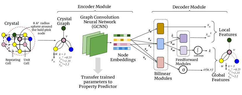
Figure 2: The architecture of the Crystal Auto Encoder (CrysAE) module which comprises multilayer graph convolution network as the encoder and a set of decoding modules for reconstructing different local and global features.

Encoder. We extend the crystal graph encoder proposed by Xie et.al. [6] to encode the chemical and structural information of a crystal graph $\mathcal{G}$. Specifically, we encode $L$-hop neighbouring information of each node as:

$$\bm{h}_{(u,v)_{k}}^{l}=\bm{z}_{u}^{l}\oplus\bm{z}_{v}^{l}\oplus{s^{k}_{(u,v)}}$$ (1)

$$\bm{z}_{u}^{l+1}=\bm{z}_{u}^{l}+\sum\limits_{v,k}\sigma({\bm{h}^{l}_{(u,v)}}_{k}\bm{W}_{c}^{(l)}+\bm{b}_{c}^{(l)})\odot g({\bm{h}^{l}_{(u,v)}}_{k}\bm{W}_{s}^{(l)}+\bm{b}_{s}^{(l)})$$

where $\bm{z}_{u}^{l}$ denotes the embedding of node $u$ after $l$ hop neighbor information aggregation. The embedding of a node $u$ is initialized to a transformed node feature vector, i.e. it is a function of the atom $u$’s chemical features as $\bm{z}_{u}^{0}:=\bm{x}_{u}\bm{W}_{x}$ where $\bm{W}_{x}$ is the trainable parameter of the transformation network and $\bm{x}_{u}$ is the input node feature vector. ${s^{k}_{(u,v)}}\in\bm{\mathcal{F}}_{u}$ represents the length of the $k^{th}$ edge between nodes $u$ and $v$. The $\oplus$ operator denotes concatenation and $\odot$ denotes element-wise multiplication. $\bm{W}_{c}^{(l)},\bm{W}_{s}^{(l)},\bm{b}_{c}^{(l)},\bm{b}_{s}^{(l)}$ are the convolution weight matrix, self weight matrix, convolution bias, self bias of $l^{th}$ hop convolution, respectively. $\sigma$ is a non-linear transformation function and it is used to generate a squeezed real value in [0,1] indicating the edge importance and $g$ is a feed forward network. After neighborhood aggregation we accumulate local information at each node which can be represented as $\bm{z}_{u}:=\bm{z}_{u}^{L}$. Subsequently we generate a graph level global information $\bm{\mathcal{Z}}=\{\bm{z}_{1},...,\bm{z}_{|\bm{\mathcal{V}}|}\}$. We do not aggregate the node embeddings further to prevent information loss in autoencoder. We denote the set of trainable parameters for this encoder as $\bm{\theta}$ for future reference.
Decoder. We design an effective decoder that helps the encoder to transform the desired information in the representation vector space of $\bm{\mathcal{Z}}$. The decoder plays an inevitable role in learning the local and global structure as well as chemical features which are extremely useful. As mentioned earlier the global chemical features i.e. the crystal properties are a function of the local chemical environment and the overall conformation of the repeating crystal cell structure; hence, we carefully design the decoder which can reconstruct two important features that induce the local chemical environment. They are (a) the node features i.e chemical properties of individual atoms and (b) local connectivity i.e the relative position of the nodes with respect to their neighbors. Precisely we reconstruct these information as below:

$$z_{uv}=\bm{z}_{u}^{T}\bm{W}_{f}\bm{z}_{v}+b_{f}$$ (2)

$$\hat{s_{(u,v)}^{k}}=\begin{cases}\gamma_{s}(z_{uv}\odot k)&\text{if }\gamma_{s}(.)>0\\ 0&\text{otherwise}\end{cases}$$ (3)

$$\bm{\mathcal{\hat{X}}}_{u}=\bm{W}_{x}^{T}\bm{z}_{u}+\bm{b}_{x}$$ (4)

Eqs. 3 and 4 correspond to reconstructing the node property or atom’s chemical property and a node’s position relative to it’s neighbors as we intend to achieve in (a) and (b) respectively. $z_{uv}$ is a combined transformed embedding of nodes $u$ and $v$ and $\gamma_{s}$ is a feed forward network which generates a real number corresponding to the length of the bonds.
Further we reconstruct the global structure i.e (c) the connectivity and periodicity of the crystal structures as below

$$(u,v)\sim p(e=(u,v))=\sigma(\bm{z}_{u}^{T}\bm{W}_{e}\bm{z}_{v}+b_{e})$$ (5)

$$k_{(u,v)}=\arg\max_{k}\frac{e^{\gamma_{k}(z_{uv},k)}}{\sum_{k}e^{\gamma_{k}(\bm{z}_{uv},k)}}$$ (6)

Here, $\bm{W}_{e},b_{e}$ are trainable weight and bias associated with the bilinear edge reconstruction module, respectively. $\sigma$ is a squashing factor which provides a value between $[0,1]$ denoting the edge probability. Similarly $\bm{W}_{f},b_{f}$ are the trainable weight and bias parameters associated with the intermediate bi-linear transformation module, respectively. $\gamma_{k}$ represents a feed forward neural network that generates a $K$ length logit vector. We use a softmax to determine the exact number of edges present. Please note that though Eqs. 6, 3 correspond to global and local information respectively, they are heavily dependent upon each other, i.e the number of bonds and bond length both depend on the two end nodes information. Hence, we design a coupled embedding $z_{uv}$ which is shared by both the modules. We denote the set of parameters in decoder as $\bm{\phi}$.
Training of auto-encoder. We learn the trainable parameters of both encoder and decoder by minimizing the reconstruction loss of different global and local structural and chemical features defined in Eqs. 3-6. We minimize the cross-entropy loss of the predicted global features and node features along with mean squared loss of the edge weight or bond length in the following objective:

$$\mathbb{E}_{\mathcal{G}\sim\bm{\mathcal{D}}}-\sum_{(u,v)\in\mathcal{E}}\big{[}\text{log}\ p(e=(u,v))+\text{log}\ p(k_{(u,v)})\big{]}$$

$$-\sum_{u\in\mathcal{V}}\text{log}\ p(\bm{\mathcal{\hat{X}}}_{u})+\sum_{(u,v)\in\mathcal{E}}\sum_{k\in[1,\dots,K]}(s^{k}_{(u,v)}-\hat{s^{k}_{(u,v)}})^{2}$$ (7)

where $p(.)$ denotes the probability of any event. Thus by minimizing the reconstruction loss we not only fine tune parameters of decoder but efficiently train the encoder to generate a rich $\bm{\mathcal{Z}}$ which facilitates decoder operations.
Property predictor (CrysXPP). Next, we design a property predictor specific to a property that can take the advantage of the structural information that is learned by the encoder as described above. We generate a graph level representation using the same graph encoder module as described in Eq.1, thus in a way transferring the rich encoded knowledge to the property predictor. Next, we use a symmetric aggregation function to generate a single vector as graph representation $\bm{\mathcal{Z}}_{g}$. Thus the obtained representation of the graph is invariant of the node orderings. Then the obtained representation is fed to a multilayer perceptron which predicts the value of the properties. More formally the property predictor can be characterized as:

$$\bm{\mathcal{Z}}_{g}=\Lambda(\bm{z}_{1}\dots,\bm{z}_{|\mathcal{V}|})$$ (8)

$$\mathcal{P}=\mathcal{M}_{\bm{\psi}}(\bm{\mathcal{Z}}_{g})$$ (9)

Here, $\Lambda$ is the aggregation function which is symmetric. $\mathcal{M}$ denotes a multilayer perceptron that has a trainable parameter set $\bm{\psi}$.
Feature Selection. The node features are first passed through a feature selector which is a trainable weight vector that selects a weighted subset of important node level features $\bm{\mathcal{X}}^{\prime}$ for a given property of interest $\mathcal{P}$. $\bm{\mathcal{X}}^{\prime}$ forms input to the encoder.

$$\bm{\mathcal{X}}^{\prime}={\mathcal{S}}_{\bm{\zeta}}(\bm{\mathcal{X}});\bm{\mathcal{Z}}_{g}=\Lambda(\text{Encoder}_{\bm{\theta^{\prime}}}(\bm{\mathcal{V}},\bm{\mathcal{E}},\bm{\mathcal{X}}^{\prime},\bm{\mathcal{F}}))$$

In the above set of characteristic equations, ${\mathcal{S}}$ is the feature selector and $\bm{\zeta}$ is its trainable weight. We will show how the weights chosen by the feature selection layer help us to explain the role of a node feature in the manifestation of a particular property (viz. formation energy) of a crystal.
Training of CrysXPP. We train the property predictor after the autoencoder. We initialize the trainable parameter $\bm{\theta}^{\prime}:=\bm{\theta}$ where $\bm{\theta}$ is trained in the autoencoding module. Thus we first transfer the trained information such that the property predictor benefits from the inductive bias already learned by training the autoencoder.
We use a LASSO [28] regression to impose sparsity on the feature selector layer. Intuitively, if some atomic features ($\bm{\mathcal{X}}^{\prime}$) are crucial to predict a chemical property of the crystal, the corresponding feature selector value will be high and conversely, if some feature is not so important, the corresponding feature selector value will be negligible. Hence, along with property prediction loss we also consider the LASSO regression loss as formally represented below:

$$\min_{\bm{\zeta},\bm{\theta^{\prime}},\bm{\psi}}(\hat{\mathcal{P}}-\mathcal{P})^{2}+\lambda_{1}*|{\bm{\zeta}}|_{L_{1}}$$ (10)

where $\bm{\zeta}$ denotes the trainable parameters of feature selector ${\mathcal{S}}$ and $\lambda_{1}$ is a hyper parameter which controls the degree of the regularization imposed. Before reporting the results, we briefly discuss about the dataset and the baselines used for comparison.

2.2 Dataset

We have used the Materials Project database for our experiments which consists of $\sim$36,835 crystalline materials and is diverse in structure having materials with 87 different types of atoms, seven different lattice systems and 216 space groups. The unit cell of any crystal can have a maximum of 200 atoms. We consider nine properties for each atom which were used to construct the feature vector of each node [6]. The details of the properties are given in Table 1. We convert them to categorical values if they are already not in that form. The dataset also provides DFT calculated target property values for the crystal structures. Experiments were done on a smaller training set than the original baseline papers.

2.3 Comparison with similar baseline algorithms

We compare the performance of CrysXPP with four state-of-the-art algorithms for crystal property prediction. These selected competing methods are varied in terms of input data processing and working paradigms as described below:

1. CGCNN [6]: This method generates crystal graphs from inorganic crystal materials and builds a graph convolution based supervised model for predicting various properties of the crystals.

2. MT-CGCNN [7] : This model uses the graph convolution based encoding as proposed in the previous model. Moreover, it incorporates multitask learning to jointly predict multiple properties of a single material.

3. MEGNET [8]: Here authors improved the CGCNN model further by introducing global state attributes including temperature, pressure, entropy etc for quantitative structure-state-property relationship prediction in materials. Doing so they found that the crystal embeddings in MEGNet model encode periodic chemical trends. Further to address the issue of data limitation the embeddings from a MEGNet model trained on formation energies is transferred and used to improve the accuracy of ML models for the band gap and elastic moduli.

4. ELEMNET [29]: This work does not specifically consider any structural properties of the crystal graph, rather it considers only the compositional atoms. It uses deep feed-forward networks to implicitly capture the effect of atoms on each other. It uses transfer learning to mitigate the error bias of DFT tagged data.

5. GATGNN [12]: In this work authors have incorporated a graph neural network with multiple graph-attention layers (GAT) and a global attention layer, which can learn efficiently the importance of different complex bonds shared among the atoms within each atom’s local neighborhood.

For all the baselines we have used the hyper parameters as mentioned in the original papers.

2.4 Evaluation criteria

We predict seven different properties of crystals in our experiments. Out of these, four are crystal state properties, namely, (a) Formation Energy, (b) Band Gap, (c) Fermi Energy, (d) Magnetic Moment, and three are elastic properties, namely, (e) Bulk Moduli, (f) Shear Moduli, and (g) Poisson Ratio. All of these properties significantly depend on the details of the crystal structure except Magnetic Moment which is more dependent on the atomic/node specifications as the magnetic moment arises from the unpaired d or f electrons in an atom. Also the size of the moment depends on the local environments  [30, 31]. Moreover, we have very little DFT tagged data for Magnetic Moment and Band Gap.
We focus on three different evaluation criteria as described below:

1. How effective is the property predictor? Here we inspect the performance of the property predictor especially when it functions with a small amount of DFT tagged data.

2. How robust is the structural encoding? Here we investigate whether the structural encoding helps us to mitigate the noise introduced by DFT calculated properties.

3. How effective is the explanation? We cross-validate the obtained explanation with domain knowledge.

	Property	Unit	CGCNN	MTCGCNN	MEGNet	GATGNN	Elemnet	CrysXPP
State Properties	Formation Energy	eV/atom	0.127	0.112 (0.147)	0.142	0.164	0.098*	0.086
	Band Gap	eV	0.503	0.497 (0.518)	0.498	0.489*	0.491	0.467
	Fermi Energy	eV	0.528	0.503* (0.601)	0.533	0.533	0.588	0.471
	Magnetic Moment	$\mu_{B}$	1.21	1.16 (1.22)	1.19	1.09	0.96	1.03*
Elastic Properties	Bulk Moduli	log(GPa)	0.09	0.09 (0.09)	0.105	0.088*	0.1057	0.08
	Shear Moduli	log(GPa)	0.125*	0.120 (0.078)	0.187	0.123	0.148	0.105
	Poisson Ratio	-	0.04	0.037* (0.039)	0.041	0.039	0.039	0.035

Table 2: Summary of the prediction performance (MAE) of different properties trained on 20% data and evaluated on $80\%$ of the data. The best performance is highlighted in bold and second best with *. We report MAE jointly training most correlated property (average on all property pairs) for MTCGCNN.

2.5 Effectiveness of Property Predictor

We first train the autoencoder with all untagged crystal graph present in the dataset, which captures all the structural information of the crystal graphs. Next for a given property of interest, we train the property predictor with 20% of the available DFT tagged data and test on the rest. We report the 10 fold cross validation results.
Metric. We report Mean Absolute Error (MAE) to compare the performance of the participating methods. MAE is defined as $\frac{1}{|\bm{\mathcal{D}}|}\sum_{\mathcal{G}\in\bm{\mathcal{D}}}\big{|}{\mathcal{P}_{\mathcal{G}}-\hat{\mathcal{P}}_{\mathcal{G}}}\big{|}$, where $\mathcal{P}_{\mathcal{G}}$ is the property value calculated by DFT and $\hat{\mathcal{P}}_{\mathcal{G}}$ is the predicted value of a graph $\mathcal{G}$.
Results. In Table 2 we report the MAE for CrysXPP as well as other alternatives on seven property values. We observe that CrysXPP outperforms every baseline across all the properties except magnetic moment. For MTCGCNN we report two values: the MAE obtained while jointly predicting the most correlated property, and the average MAE across all possible combinations (in bracket). It is interesting to note that its performance significantly degrades if the other property is not correlated with the current property of interest. A careful inspection reveals that for elastic properties, graph neural network based methods perform better than that of Elemnet. Elemnet only considers the composition of the crystal and ignores the global structural information, whereas these properties heavily depend on the crystal structure. In contrast, for Magnetic Moment the local information is important and hence, Elemnet performs the best and CrysXPP is the second best method. For the rest of the crystal state based properties, there is no consistent second best method. However, CrysXPP is a clear winner with a considerable margin which is due to the fact that the property predictor benefits from the structural knowledge transferred from the autoencoder.
Behaviour with increase in tagged data. Further, we check the robustness of CrysXPP, by increasing the percentage of tagged training data for property prediction. We report the behavior of CrysXPP as well as other baselines in Fig.3 for all the properties. We observe a monotonic decrease of MAE between predicted and DFT calculated vales for most of the models where CrysXPP yields consistently smaller MAE and maintains the leadership position for all the properties expect Magnetic Moment. This shows the robustness of our model to be able to perform consistently across a diverse set of properties with varied training instances. The MAE margin between CrysXPP and closest competitor (which is variable across properties), however, reduces as training size increases. For Magnetic Moment, the local chemical information is more vital, hence ElemNet, which concentrate more on local chemical information, shows the best performance.

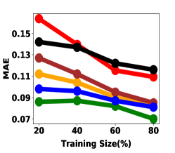
(a) Formation Energy

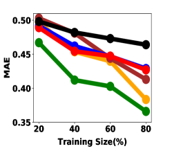
(b) Band Gap

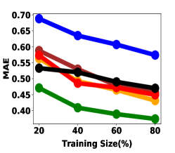
(c) Fermi Energy

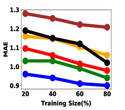
(d) Magnetic Moment

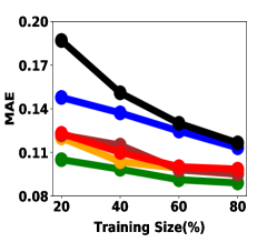
(e) Shear Moduli

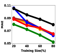
(f) Bulk Moduli

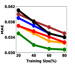
(g) Poisson Ratio

Figure 3: Variation of MAE with the increase in training instances from 20% to 80%. CrysXPP outperforms all the baselines consistently.

2.6 Removal of DFT error bias

An important aspect of the prediction is that since we rely only on DFT data for training, we would be limited by the inaccuracies of DFT. In this section, we investigate with a system where we further fine tune the model with a small amount of available experimental data and check whether the system can remove the error propagated due to DFT.
Calculation setup. We consider a property predictor (as explained before) which has been trained with crystals whose particular property (e.g. Band Gap) values have been theoretically derived using DFT. We then fine tune the parameters with limited amount of experimental data; we perform it for two different properties, namely, Band Gap and Formation Energy. For Formation Energy, we use 1,500 instances available at [22] and use different percentages of the data to fine-tune the model parameters. For Band Gap, we collect 20 experimental instances out of which we randomly pick 10 instances to fine-tune the parameters and report the prediction value for the rest  .

Experiment Settings	CGCNN	MTCGCNN	GATGNN	MEGNet	ElemNet	CrysXPP
Train on 20% DFT Test on Full Experimental Data	0.24	0.74	0.30	0.28	0.215	0.22
Train on 20% DFT, 20 % Experimental Data Test on 80 % Experimental Data	0.21	0.24	0.23	0.23	0.16*	0.15 (0.206)
Train on 80% DFT, 20 % Experimental Data Test on 80 % Experimental Data	0.16	0.22	0.19	0.18	0.1344*	0.1319 (0.195)
Train on 80% DFT, 80 % Experimental Data Test on 20 % Experimental Data	0.12	0.15	0.13	0.125	0.0905*	0.0892 (0.174)

Table 3: MAE of predicting experimental values after fine tuning different methods with different percentages of experimental data for formation energy. MAE of the experiment where we replace the experimental data with the same amount of DFT data to train CrysXPP, is provided in the bracket. The closest prediction is marked in bold and second best with *.

Materials	Exp	DFT	CrysXPP	CGCNN	MTCGCNN	GATGNN	MEGNet	ElemNet
GaSb	0.72	0.36	0.77 (0.9*)	1.01 (4.27)	0.26 (0.06)	3.78(1.58)	2.26(1.31)	1.09 (0.33)
GaP	2.26	1.69	2.10 (1.86)	1.95* (1.49)	0.73 (0.64)	2.77(0.08)	1.21(2.51)	2.80 (1.29)
GaAs	1.42	0.18	1.54* (1.56)	2.51 (1.42)	1.83 (1.90)	2.73(3.50)	0.77(0.98)	0.83 (0.76)
InN	1.97	0.47	1.92 (1.85*)	1.30 (2.90)	1.77 (2.30)	2.79(0.08)	1.33(2.16)	1.64 (1.43)
GaN	3.2	1.73	2.11 (1.47)	3.51* (1.55)	0.28 (0.16)	2.27(0.56)	1.59(2.66)	3.69 (1.44)
NiO	4.3	2.214	2.45 (2.08)	0.96 (1.12)	0.08 (0.05)	2.12(1.36)	2.01(2.71)	2.31* (1.88)
Si	1.12	0.85	1.08 (0.95*)	1.56 (1.64)	0.39 (0.22)	3.60(0.31)	1.86(1.69)	0.33 (0.17)
ZnO	3.37	1.05	3.42* (2.1)	3.32 (1.45)	0.83 (0.56)	2.74(1.36)	2.09(2.53)	2.55 (2.01)
FeO	2.4	0	2.25 (1.72)	2.16* (2.85)	1.12 (0.96)	1.92(1.02)	2.93(2.81)	1.44 (1.27)
MnO	4	0.20	2.31 (1.81)	1.51 (1.22)	1.04 (0.77)	2.44(2.35)	1.73(2.11)	1.98* (1.44)

Table 4: Experiment (Exp) and predicted value for Band Gap for 10 crystals calculated by DFT and other machine learning models after fine-tuned by experimental data. The predicted value without fine tuning by experimental data is provided in the bracket.The closest prediction is marked in bold and the second best with *. CrysXPP predicts closest to the ground truth after fine tuning with experimental data.

Results (Formation Energy). We report the mean absolute error (MAE) of Formation Energy in Table 3 achieved by different methods. The DFT prediction of the Formation Energy on the 1,500 crystals has an MAE of 0.21 with respect to experimental data and by training our model with DFT data we are performing close to the performance achieved by DFT. The results have a consistent trend for all the methods, whereby we observe that increasing the amount of training data, even if that is error-prone DFT data, helps in minimizing MAE. CrysXPP performs consistently better by a large margin than CGCNN and MTCGCNN, which takes the graph structure as an explicit input. However, it is interesting to observe that ElemNet performs very close to CrysXPP as Formation Energy depends more on the composition than that on the explicit connection of atoms. Further, we conduct an experiment where we replace the experimental data with the same amount of DFT data to train our model. We then evaluate the performance of the model using experimental data as test data and find an inferior performance. We report the results in Table 3 (last column (in bracket)).
Results (Band Gap). In Table 4 we report the experimental value of Band Gap for 10 test instances along with the predicted values by DFT and other machine learning methods. The error margin of DFT with the actual experimental values is quite high. It is interesting to see that other than a few, DFT prediction is far from experimental data and in most of the cases, it is underestimating the experimental values. After fine-tuning DFT trained machine learning models with experimental data, the prediction becomes closer to the experimental value. However, CrysXPP performs closest to the experimental result in almost all the cases in comparison to other alternatives. ElemNet, although second on the average when trained only on DFT (row 2 of Table 2), cannot consistently maintain that position, whereas CGCNN performs better. We have also provided results (in bracket) when we do not do any fine tuning. It can be seen even in such a scenario in many of the cases the performance is better than DFT. Further the power of CrysXPP in quickly mitigating the bias of DFT when fine-tuned on minuscule data shows the usefulness of modeling explicit structural information.

Property Name	Ablation Settings	Train-Test Split
		20% - 80%	40% - 60%	60% - 40%	80% - 20%
Formation Energy	Without Global + Local effect	0.124	0.113	0.092	0.086
	Global effect	0.112	0.092	0.085	0.077
	Local effect	0.079	0.067	0.063	0.061
	CrysXPP	0.086	0.082	0.076	0.067
Band Gap	Without Global + Local effect	0.502	0.482	0.452	0.408
	Global effect	0.479	0.425	0.393	0.382
	Local effect	0.471	0.419	0.387	0.375
	CrysXPP	0.467	0.402	0.383	0.366
Fermi Energy	Without Global + Local effect	0.513	0.481	0.477	0.443
	Global effect	0.495	0.476	0.441	0.437
	Local effect	0.488	0.472	0.436	0.428
	CrysXPP	0.471	0.409	0.389	0.374
Magnetic Moment	Without Global + Local effect	1.082	1.038	1.023	1.027
	Global effect	1.072	1.066	1.027	1.019
	Local effect	1.068	1.052	1.022	1.013
	CrysXPP	1.033	1.024	0.997	0.943
Bulk Moduli	Without Global + Local effect	0.091	0.088	0.081	0.075
	Global effect	0.088	0.081	0.075	0.068
	Local effect	0.087	0.077	0.072	0.063
	CrysXPP	0.080	0.072	0.063	0.052
Shear Moduli	Without Global + Local effect	0.122	0.119	0.106	0.098
	Global effect	0.119	0.108	0.099	0.093
	Local effect	0.117	0.102	0.097	0.091
	CrysXPP	0.105	0.098	0.091	0.089
Poisson Ratio	Without Global + Local effect	0.039	0.035	0.033	0.032
	Global effect	0.037	0.034	0.032	0.031
	Local effect	0.037	0.033	0.031	0.031
	CrysXPP	0.035	0.032	0.031	0.030

Table 5: Summary of experiments of ablation study on importance of different reconstruction loss components on CrysAE training and eventually its effect on CrysXPP (MAE for property prediction).

Property Name	Ablation Settings	Train-Test Split
		20% - 80%	40% - 60%	60% - 40%	80% - 20%
Formation Energy	Without $L_{1}$ regularizer	0.092	0.089	0.083	0.0731
	With $L_{1}$ regularizer	0.086	0.082	0.076	0.067
Band Gap	Without $L_{1}$ regularizer	0.476	0.417	0.391	0.374
	With $L_{1}$ regularizer	0.467	0.402	0.383	0.366
Fermi Energy	Without $L_{1}$ regularizer	0.502	0.441	0.415	0.394
	With $L_{1}$ regularizer	0.471	0.409	0.389	0.374
Magnetic Moment	Without $L_{1}$ regularizer	1.094	1.046	1.028	1.013
	With $L_{1}$ regularizer	1.033	1.024	0.997	0.943
Bulk Moduli	Without $L_{1}$ regularizer	0.093	0.082	0.067	0.061
	With $L_{1}$ regularizer	0.080	0.072	0.063	0.052
Shear Moduli	Without $L_{1}$ regularizer	0.128	0.115	0.099	0.095
	With $L_{1}$ regularizer	0.105	0.098	0.091	0.089
Poisson Ratio	Without $L_{1}$ regularizer	0.038	0.033	0.033	0.032
	With $L_{1}$ regularizer	0.035	0.032	0.031	0.030

Table 6: Summary of experiments of ablation study on sparse feature selection using $L_{1}$ regularizer, performed on different train test splits across different properties (MAE).

Property Name	Ablation Settings	Train-Test Split
		20% - 80%	40% - 60%	60% - 40%	80% - 20%
Formation Energy	GCN Encoder	0.187	0.162	0.138	0.125
	CGCNN Encoder	0.086	0.082	0.076	0.067
Band Gap	GCN Encoder	0.613	0.515	0.493	0.476
	CGCNN Encoder	0.467	0.402	0.383	0.366
Fermi Energy	GCN Encoder	0.513	0.489	0.450	0.436
	CGCNN Encoder	0.471	0.409	0.389	0.374
Magnetic Moment	GCN Encoder	1.204	1.113	1.080	1.041
	CGCNN Encoder	1.033	1.024	0.997	0.943
Bulk Moduli	GCN Encoder	0.171	0.133	0.114	0.101
	CGCNN Encoder	0.080	0.072	0.063	0.052
Shear Moduli	GCN Encoder	0.183	0.172	0.168	0.141
	CGCNN Encoder	0.105	0.098	0.091	0.089
Poisson Ratio	GCN Encoder	0.041	0.037	0.036	0.034
	CGCNN Encoder	0.035	0.032	0.031	0.030

Table 7: Summary of experiments (MAE) of ablation study on effect of GCN as graph encoder in CrysAE and CrysXPP.

2.7 Ablation Studies

We demonstrate the effectiveness of architectural choices and training strategies for CrysXPP, by designing the following set of ablation studies:

1. The importance of explicitly capturing global and local features and understanding their effect on property prediction

2. The impact of sparse feature selection on property prediction, and

3. The choice of GNN models in the autoencoder CrysAE

In the following subsections we will thoroughly discuss these.
Importance of local and global feature understanding. Here we investigate the importance of different reconstruction loss components on CrysAE training and eventually its effect on property prediction. (a). Without Global + Local effect : In this scenario we do not train CrysAE and only train CrysXPP. (b). Global effect : We train CrysAE by minimizing the reconstruction loss of only global features and ignoring local feature losses. (c). Local effect: Here we focus only minimizing local feature losses. We report the performance of the model (MAE) in Table 5 on different train test splits across different properties. We observe that the performance of the model in the setting Without Global + Local effect, is the worst. We also notice that for all the properties, Local effect individually leads to better performance than Global effect, except for the Poisson ratio where the effect is similar for both the cases. However, it is found that the impact of local and global effect are somewhat complementary, hence simultaneous reconstruction of global and local features (CrysXPP) results in the best performance. The only exception is formation energy where addition of global feature leads to performance deterioration..
Impact of sparse feature selection. We perform an ablation study to analyze the impact of sparse feature selection on property prediction. This is done by removing the $L_{1}$ regularizer term from CrysXPP loss function in Eq.10. We evaluate the performance of the model and report the results (MAE) in Table 6. We observe discernible improvement due to the introduction of sparse feature selection using $L_{1}$ regularizer.

Effect of other GNN variants as graph encoder. To explore the effectiveness of other GNN variants as graph encoders, we conduct an experiment where we replace the CGCNN encoder with one of the popular GNN variants: GCN [33] encoder and evaluate the performance of the model. GCN only considers the graph structural information and atom features to learn the graph representation and unlike CGCNN, it does not consider the individual edges weights in the multi-graph representing a crystal. We report the results of the model performance (MAE) in Table 7. We observe that the model performance degrades when trained with GCN. The edge weight calculation, which is a major contribution of CGCNN, is extremely helpful to capture the local structure of the crystal.

2.8 Explanation through feature selection

We have introduced a feature selector that is trained along with the property prediction parameters with available tagged data. The feature selector helps to select the subset of the atomic features contributing to the chemical properties of the crystal which makes the model explainable by design. To demonstrate the effectiveness of the feature selector, we have selected few case studies and provide the feature explanation for formation energy, band gap and magnetic moment.

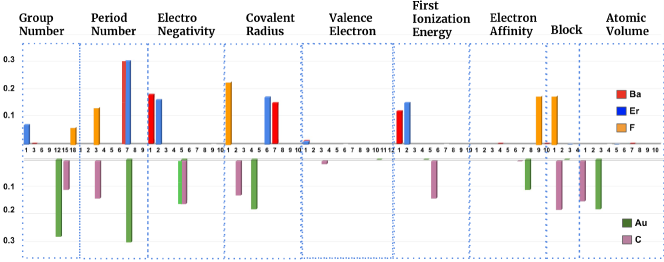
Figure 4: Feature selector values corresponding to atom features after trained on Formation Energy tagged data. The top bar chart represents the feature weights of $BaEr_{2}F_{8}$ and the below one represents the feature weights of AuC.

Formation Energy. We here report case studies corresponding to two crystals $BaEr_{2}F_{8}$ and AuC, illustrating the important role of feature selector in providing explanation. We report the feature selector values corresponding to categorical atomic properties after being trained on Formation Energy tagged data in Fig.4. The bars represent the weights assigned by the feature selector on the categorical values of atomic features and different colors indicate different atoms. Higher category denotes higher value of the feature. Fig.4 depicts the importance of the atomic features in two extreme cases. One is $BaEr_{2}F_{8}$, whose Formation Energy is predicted as -4.41 eV/atom indicating its stability while the other is AuC with predicted Formation Energy 2.2 eV/atom denoting the material is quite unstable. In both cases we see that Period Number is the most important atomic feature as it has maximum weight. Period and Group Numbers provide the information to distinguish each element. As the Group Numbers and the number of Valence Electrons are closely related, we see that the feature selector only selected the former thus avoiding duplicity. Electronegativity and Covalent Radius both are another two important features (with non-zero weight) which is evident from the figure. Non-zero difference in Electronegativity of atoms indicates stability in structure. Both Au and C have the same Electronegativity (category value 5), and feature selector gives same weight to it, as a result the difference of Electronegativity is zero in the case of unstable AuC. While for the case of stable $BaEr_{2}F_{8}$, the feature selector provides different non-zero weights to smaller Electronegative elements and zero weight to the largest Electronegative atom F. The Covalent Radius determines the extent of overlap of electron densities of constituents, therefore, it appeared as another important feature. Higher the radius means weaker the bond. It is interesting to note here the trend of weights is the reverse than that of radius itself (Ba has the largest radius 215 pm and has the smallest weight) for stable $BaEr_{2}F_{8}$. The scenario is reverse for unstable AuC. Ionization Energy plays similar role as Electronegativity and we observe same behavior of feature selector. As can be seen from the example, the feature selector provides elaborate cues for domain experts to reason out the results.

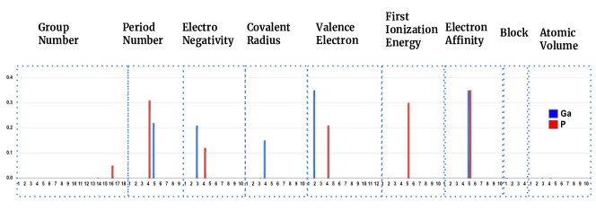
Figure 5: Feature selector values corresponding to atom features after trained on Band Gap tagged data. The top bar chart represents the feature weights of GaP (Band Gap 2.26 eV).

Band Gap. In Fig.5, we show the important features that appear in the case of band gap. It is interesting to see that the Electron Affinity came out to be the most important atomic feature for the band gap as it determines the location of conduction band minimum with respect to the vacuum. Again, as the number of Valence Electrons and the group number are collinear properties, only one (valence electrons) is found to be having the significant weight. The Conduction Band is composed of Ga-states while the valence band is composed of P states with small admixture of Ga-states, that gives Ga-valence electrons more weight. The situation is reversed for the Ionization Energy, which determines the location of the valence band with respect to a vacuum, and as the valence band is mostly formed by the P atom, we see P has more weight.

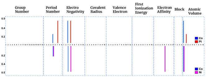
Figure 6: Feature selector values corresponding to atom features after trained on Magnetic Moment tagged data. The top bar chart represents the feature weights of CoPt and the bottom chart represents the feature weights of CoNi.

Magnetic Moment. In order to understand the feature importance in the case of magnetic moment, we compare the results obtained for two Co based alloys, namely, CoPt and CoNi (Fig.6). In both cases the Atomic Volume, Period Number and Electronegativity appear to be the three most important features. While in the case of CoNi, Electron Affinity of Ni also appeared to be as additional important feature. It can be seen that in the case of CoPt, the Atomic Volume of Co has higher weight, while for CoNi, the atomic volume for both the species have the same weight. This is quite intuitive, as for CoPt, the magnetic moment is mostly carried by Co atom, while in the case of CoNi, both the atoms have significant contribution. The Electronegativity plays an important role in the context of magnetic moment. For example the magnetic moment of Co in CoPt is slightly higher than its corresponding value in pure Co. The electronegativity difference between Co and Pt causes the electron transfer from Co minority spin band to Pt which in turn enhances its magnetic moment [31, 34]. In the case of Period Number again we see that for CoPt, it is only the period number of the magnetic atom, i.e, the Co atom that is given visible weight while in the case of NiCo, the period number of the two atoms appears to be important.
It is evident from the above analysis that CrysXPP is effectively constructing models where the important node features are physically intuitive.
In conclusion, we propose an explainable property predictor for crystalline materials, CrysXPP to predict different crystal state and elastic properties with accurate precision using small amount of property-tagged data. We address the issue of limited crystal data where the value of a particular property is known, using transfer learning from an encoding module CrysAE; which we train in a property agnostic way with a large amount of untagged crystal data to capture all the important structural and chemical information useful to a specific property predictor. We further find the encoder knowledge is extremely useful in de-biasing DFT error using a meagre instances of experimental results. CrysXPP outperforms all the baselines across seven diverse sets of properties. With appropriate case studies, we show that the explanations provided by the feature selection module are in sync with the domain knowledge. We release the large pretrained model CrysAE so that it could be fine-tuned using a small amount of tagged data by the research community on various applications with restricted data source.

3 Methods

3.1 Hyperparameters

We have trained our model with varying convolution layers of encoder module and obtained the best results with three convolution layers in the encoder module. We kept the embedding dimension for each node as 64, batch size of data as 512 and used average pooling to obtain $\bm{\mathcal{Z}}_{g}$. We selected $\lambda=0.01$ for property selection. We varied the learning rate in logarithmic scale and selected 0.03 which yields faster convergence. We trained the auto-encoder for 200 epochs and property predictor for 200 epochs.

4 Data availability

Most of the data used were from materials project. A small section of experimental data used as ground truth and as means to reduce the DFT bias will be available upon request to the corresponding authors.

5 Code availability

Source code of CrysAE and CrysXPP is available in the following github repo:
https://github.com/iitkgpaiforscience/Crysxpp.git

6 competing interests

The authors declare no competing interests.

7 Author Contributions

SB and NG conceived the idea, SCL and PG reviewed and helped to refine it. The model was developed by KD and BS, who also built the necessary codes. The first draft of the manuscript was written by KD, with contributions from BS. The paper was reviewed and approved by all authors, who all contributed to the final version of the manuscript.

8 Corresponding authors

Correspondence to Niloy Ganguly, Satadeep Bhattacharjee and Seung Cheol Lee.

9 References

References

- [1] Seko, A. et al. Prediction of low-thermal-conductivity compounds with first-principles anharmonic lattice-dynamics calculations and bayesian optimization. Phys. Rev. Lett. 115, 205901 (2015).
- [2] Xue, D. et al. Accelerated search for materials with targeted properties by adaptive design. Nat. Commun. 7, 1–9 (2016).
- [3] Isayev, O. et al. Universal fragment descriptors for predicting properties of inorganic crystals. Nat. Commun. 8, 1–12 (2017).
- [4] Ghiringhelli, L. M., Vybiral, J., Levchenko, S. V., Draxl, C. & Scheffler, M. Big data of materials science: critical role of the descriptor. Phys. Rev. Lett. 114, 105503 (2015).
- [5] Isayev, O. et al. Materials cartography: representing and mining materials space using structural and electronic fingerprints. Chem. Mater. 27, 735–743 (2015).
- [6] Xie, T. & Grossman, J. C. Crystal graph convolutional neural networks for an accurate and interpretable prediction of material properties. Phys. Rev. Lett. 120, 145301 (2018).
- [7] Sanyal, S. et al. Mt-cgcnn: Integrating crystal graph convolutional neural network with multitask learning for material property prediction. Preprint at https://arxiv.org/abs/1811.05660 (2018).
- [8] Chen, C., Ye, W., Zuo, Y., Zheng, C. & Ong, S. P. Graph networks as a universal machine learning framework for molecules and crystals. Chem. Mater. 31, 3564–3572 (2019).
- [9] Meredig, B. et al. Combinatorial screening for new materials in unconstrained composition space with machine learning. Phys. Rev. B 89, 094104 (2014).
- [10] Jha, D. et al. Elemnet: Deep learning the chemistry of materials from only elemental composition. Sci. Rep. 8, 1–13 (2018).
- [11] Choudhary, K., DeCost, B. & Tavazza, F. Machine learning with force-field-inspired descriptors for materials: Fast screening and mapping energy landscape. Phys. Rev. Mater. 2, 083801 (2018).
- [12] Louis, S.-Y. et al. Global attention based graph convolutional neural networks for improved materials property prediction. Preprint at https://arxiv.org/abs/2003.13379 (2020).
- [13] Cheng, J., Zhang, C. & Dong, L. A geometric-information-enhanced crystal graph network for predicting properties of materials. Commun. Mater. 2, 1–11 (2021).
- [14] Banjade, H. R. et al. Structure motif–centric learning framework for inorganic crystalline systems. Sci. Adv. 7, eabf1754 (2021).
- [15] Jin, W., Barzilay, R. & Jaakkola, T. Hierarchical generation of molecular graphs using structural motifs. In International Conference on Machine Learning, 4839–4848 (PMLR, 2020).
- [16] Qiao, Z., Welborn, M., Anandkumar, A., Manby, F. R. & Miller III, T. F. Orbnet: Deep learning for quantum chemistry using symmetry-adapted atomic-orbital features. J. Chem. Phys. 153, 124111 (2020).
- [17] Ye, S., Liang, J., Liu, R. & Zhu, X. Symmetrical graph neural network for quantum chemistry with dual real and momenta space. J. Phys. Chem. A 124, 6945–6953 (2020).
- [18] Kubaschewski, O., Alcock, C. B. & Spencer, P. Materials thermochemistry. revised. Pergamon Press Ltd, Headington Hill Hall, Oxford OX 3 0 BW, UK, 1993. 363 (1993).
- [19] Bracht, H., Stolwijk, N. & Mehrer, H. Properties of intrinsic point defects in silicon determined by zinc diffusion experiments under nonequilibrium conditions. Phys. Rev. B 52, 16542 (1995).
- [20] Turns, S. R. Understanding nox formation in nonpremixed flames: experiments and modeling. Prog. Energy Combust. Sci. 21, 361–385 (1995).
- [21] Ceder, G. & Persson, K. The materials project: A materials genome approach. DOE Data Explorer (2010).
- [22] Kirklin, S. et al. The open quantum materials database (oqmd): assessing the accuracy of dft formation energies. Npj Comput. Mater. 1, 1–15 (2015).
- [23] Park, C. W. & Wolverton, C. Developing an improved crystal graph convolutional neural network framework for accelerated materials discovery. Phys. Rev. Mater. 4, 063801 (2020).
- [24] Perdew, J. P. Density functional theory and the band gap problem. Int. J. Quantum Chem. 28, 497–523 (1985).
- [25] Kannemann, F. O. & Becke, A. D. van der waals interactions in density-functional theory: intermolecular complexes. J. Chem. Theory Comput. 6, 1081–1088 (2010).
- [26] Ward, L., Agrawal, A., Choudhary, A. & Wolverton, C. A general-purpose machine learning framework for predicting properties of inorganic materials. Npj Comput. Mater. 2, 1–7 (2016).
- [27] Wu, Z. et al. Moleculenet: a benchmark for molecular machine learning. Chem. Sci. 9, 513–530 (2018).
- [28] Li, F., Yang, Y. & Xing, E. P. From lasso regression to feature vector machine. In Advances in neural information processing systems, 779–786 (2006).
- [29] Jha, D. et al. Enhancing materials property prediction by leveraging computational and experimental data using deep transfer learning. Nat. Commun. 10, 1–12 (2019).
- [30] Gerasimov, A., Nordström, L., Khmelevskyi, S., Mazurenko, V. V. & Kvashnin, Y. O. Nature of the magnetic moment of cobalt in ordered feco alloy. J. Condens. Matter Phys. 33, 165801 (2021).
- [31] Bhattacharjee, S., Yoo, S., Waghmare, U. V. & Lee, S. Nh3 adsorption on ptm (fe, co, ni) surfaces: Cooperating effects of charge transfer, magnetic ordering and lattice strain. Chem. Phys. Lett. 648, 166–169 (2016).
- [32] http://matprop.ru.
- [33] Kipf, T. N. & Welling, M. Semi-supervised classification with graph convolutional networks. In International Conference on Learning Representations (ICLR) (2017).
- [34] Bhattacharjee, S. et al. Site preference of nh 3-adsorption on co, pt and copt surfaces: the role of charge transfer, magnetism and strain. Physical Chemistry Chemical Physics 17, 9335–9340 (2015).