Mixture models for the analysis, edition, and synthesis of continuous time series

Abstract

This chapter presents an overview of techniques used for the analysis, edition, and synthesis of continuous time series, with a particular emphasis on motion data. The use of mixture models allows the decomposition of time signals as a superposition of basis functions. It provides a compact representation that aims at keeping the essential characteristics of the signals. Various types of basis functions have been proposed, with developments originating from different fields of research, including computer graphics, human motion science, robotics, control, and neuroscience. Examples of applications with radial, Bernstein and Fourier basis functions are presented, with associated source codes to get familiar with these techniques.

1 Introduction

The development of techniques to process continuous time series is required in various domains of application, including computer graphics, human motion science, robotics, control, and neuroscience. These techniques need to cover various purposes, including the encoding, modeling, analysis, edition, and synthesis of time series (sometimes needed simultaneously). The development of these techniques is also often governed by additional important constraints such as interpretability and reproducibility. These heavy requirements motivate the use of mixture models, effectively leveraging the formalism and ubiquity of these models.

The first part of this chapter reviews decomposition techniques based on radial basis functions (RBFs) and locally weighted regression (LWR). The connections between LWR and Gaussian mixture regression (GMR) are discussed, based on the encoding of time series as Gaussian mixture models (GMMs). I will show how this mixture modeling principle can be extended to a weighted superposition of Bernstein basis functions, often known as Bézier curves. The aim is to examine the connections with mixture models and to highlight the generative aspects of these techniques. In particular, this link exposes the possibility of representing Bézier curves with higher order Bernstein polynomials. I then discuss the decomposition of time signals as Fourier basis functions, by showing how a mixture of Gaussians can leverage the multivariate Gaussian properties in the spatial and frequency domains. Finally, I show that these different decomposition techniques can be represented as time series distributions through a probabilistic movement primitives representation.

Pointers to various practical applications are provided for further readings, including the analysis of biological signals in the form of multivariate continuous time series, the development of computer graphics interfaces to edit trajectories and motion paths for manufacturing robots, the analysis and synthesis of periodic human gait data, or the generation of exploratory movements in mobile platforms with ergodic control.

The techniques presented in this chapter are described with a uniform notation that does not necessarily follow the original notation. The goal is to tie links between these different techniques, which are often presented in isolation of the more general context of mixture models. Matlab codes accompany the chapter pbd (Accessed: 2019/04/18), with full compatibility with GNU Octave.

2 Movement primitives

The term movement primitives refers to an organization of continuous motion signals in the form of a superposition in parallel and in series of simpler signals, which can be viewed as “building blocks” to create more complex movements, see Fig. 1. This principle, coined in the context of motor control Mussa-Ivaldi et al. (1994), remains valid for a wide range of continuous time signals (for both analysis and synthesis). Next, I present three popular families of basis functions that can be employed for time series decomposition.

2.1 Radial basis functions (RBFs)

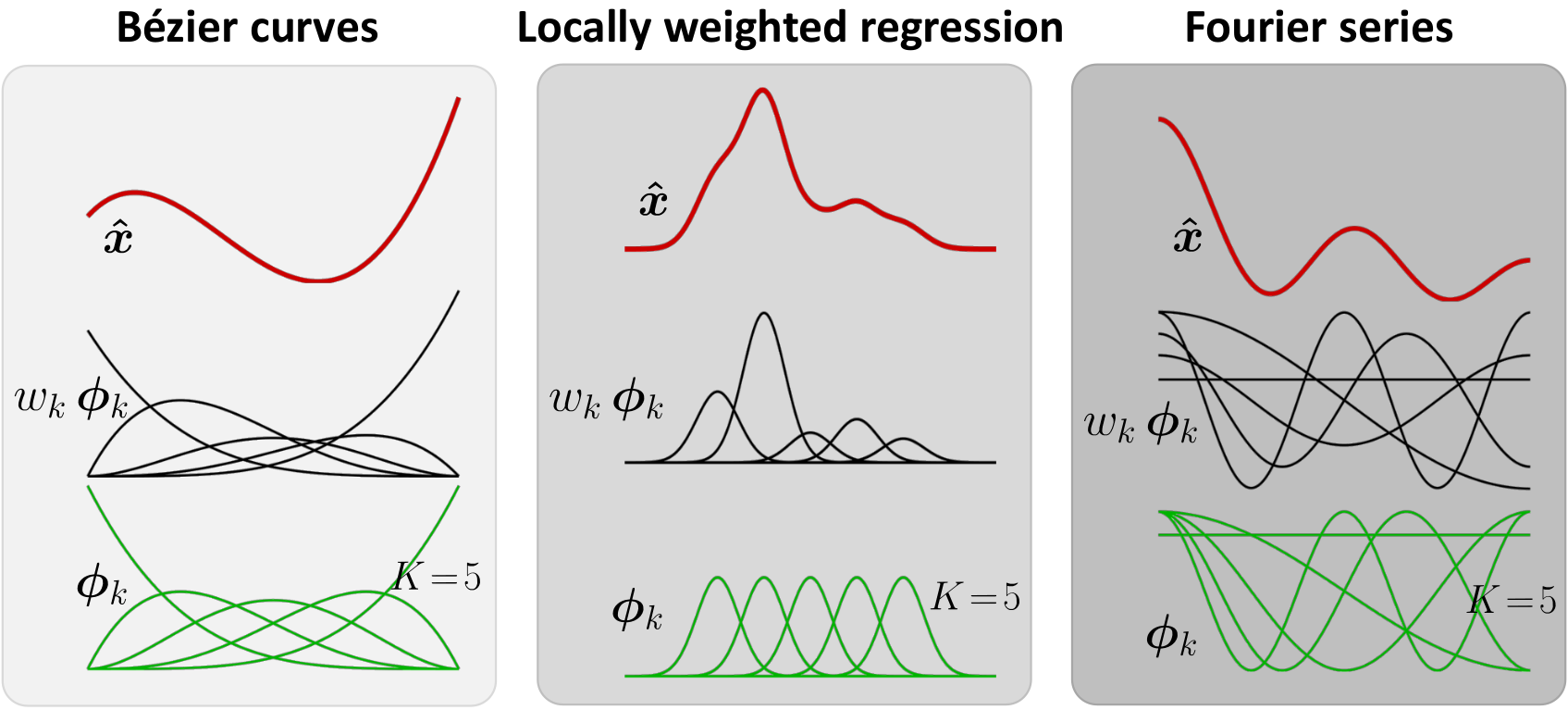
Figure 1: Motion primitives with different basis functions $\phi_{k}$, where a unidimensional time series $\bm{\hat{x}}=\sum_{k=1}^{K}w_{k}\phi_{k}$ is constructed as a weighted superposition of $K$ signals $\phi_{k}$.

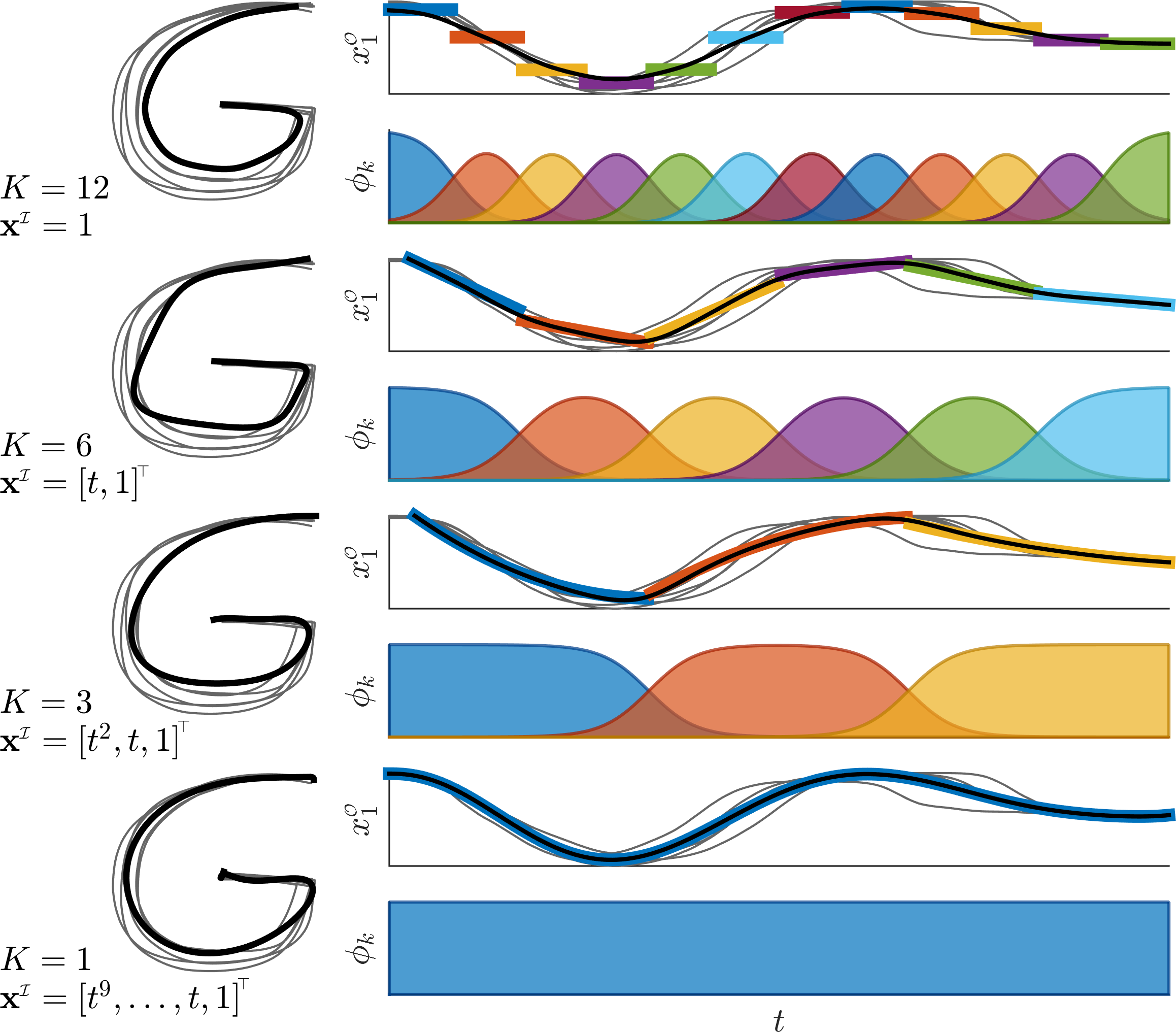
Figure 2: Polynomial fitting with locally weighted regression (LWR), by considering different degrees of the polynomial and by adapting the number of basis functions accordingly. The top row shows a very localized encoding of the movement, with constant values used in Eq. (1), thus requiring the use of many basis functions to represent the trajectory. In the top timeline graph, the colored horizontal segments can also be interpreted as scalar weights used to approximate the original signal by a weighted superposition of radial basis functions (see example in Fig. 1). The next rows show that a reduction of this number of basis functions typically needs to be compensated with more complex basis functions (polynomial of higher degrees). The bottom row depicts the limit case in which a global encoding of the movement would require a polynomial of high degree.

Radial basis functions (RBFs) are ubiquitous in continuous time series encoding Stulp and Sigaud (2015), notably due to their simplicity and ease of implementation. Most algorithms exploiting this representation rely on some form of regression, often related to locally weighted regression (LWR), which was introduced by Cleveland (1979) in statistics and popularized by Atkeson (1989) in robotics. By representing, respectively, $N$ input and output datapoints as $\bm{X}^{\scriptscriptstyle{I}}={[\bm{x}_{1}^{\scriptscriptstyle{I}},\bm{x}_{2}^{\scriptscriptstyle{I}},\ldots,\bm{x}_{N}^{\scriptscriptstyle{I}}]}^{\scriptscriptstyle\top}$ and $\bm{X}^{\scriptscriptstyle{O}}={[\bm{x}_{1}^{\scriptscriptstyle{O}},\bm{x}_{2}^{\scriptscriptstyle{O}},\ldots,\bm{x}_{N}^{\scriptscriptstyle{O}}]}^{\scriptscriptstyle\top}$, we are interested in the problem of finding a matrix $\bm{A}$ so that $\bm{X}^{\scriptscriptstyle{I}}\bm{A}$ would match $\bm{X}^{\scriptscriptstyle{O}}$ by considering different weights on the input–output datapoints $\{\bm{X}^{\scriptscriptstyle{I}},\bm{X}^{\scriptscriptstyle{O}}\}$ (namely some datapoints are more informative than others for the estimation of $\bm{A}$). A weighted least squares estimate $\bm{\hat{A}}$ can be found by solving the objective

$$\bm{\hat{A}} =\arg\underset{\bm{A}}{\min}\;\mathrm{tr}\Big{(}{(\bm{X}^{\scriptscriptstyle{O}}-\bm{X}^{\scriptscriptstyle{I}}\bm{A})}^{\scriptscriptstyle\top}\bm{W}(\bm{X}^{\scriptscriptstyle{O}}-\bm{X}^{\scriptscriptstyle{I}}\bm{A})\Big{)}$$

$$={({\bm{X}^{\scriptscriptstyle{I}}}^{{\scriptscriptstyle\top}}\bm{W}\bm{X}^{\scriptscriptstyle{I}})}^{-1}{\bm{X}^{\scriptscriptstyle{I}}}^{{\scriptscriptstyle\top}}\bm{W}\,\bm{X}^{\scriptscriptstyle{O}},$$ (1)

where $\bm{W}\!\in\!\mathbb{R}^{N\!\times\!N}$ is a weighting matrix. Locally weighted regression (LWR) is a direct extension of the weighted least squares formulation in which $K$ weighted regressions are performed on the same dataset $\{\bm{X}^{\scriptscriptstyle{I}},\bm{X}^{\scriptscriptstyle{O}}\}$. It aims at splitting a nonlinear problem so that it can be solved locally by linear regression. LWR computes $K$ estimates $\bm{\hat{A}}_{k}$, each with a different function $\phi_{k}(\bm{x}^{\scriptscriptstyle{I}}_{n})$, classically defined as the radial basis functions

$$\tilde{\phi}_{k}(\bm{x}^{\scriptscriptstyle{I}}_{n})=\exp\Big{(}\!-\frac{1}{2}{(\bm{x}^{\scriptscriptstyle{I}}_{n}-\bm{\mu}^{\scriptscriptstyle{I}}_{k})}^{\scriptscriptstyle\top}{\bm{\Sigma}^{\scriptscriptstyle{I}}_{k}}^{-1}(\bm{x}^{\scriptscriptstyle{I}}_{n}-\bm{\mu}^{\scriptscriptstyle{I}}_{k})\Big{)},$$ (2)

where $\bm{\mu}^{\scriptscriptstyle{I}}_{k}$ and $\bm{\Sigma}^{\scriptscriptstyle{I}}_{k}$ are the parameters of the $k$-th RBF, or in its rescaled form

$$\phi_{k}(\bm{x}^{\scriptscriptstyle{I}}_{n})=\frac{\tilde{\phi}_{k}(\bm{x}^{\scriptscriptstyle{I}}_{n})}{\sum_{i=1}^{K}\tilde{\phi}_{i}(\bm{x}^{\scriptscriptstyle{I}}_{n})}.$$ (3)

An associated diagonal matrix

$$\bm{W}_{k}=\mathrm{diag}\Big{(}\phi_{k}(\bm{x}^{\scriptscriptstyle{I}}_{1}),\phi_{k}(\bm{x}^{\scriptscriptstyle{I}}_{2}),\ldots,\phi_{k}(\bm{x}^{\scriptscriptstyle{I}}_{N})\Big{)}$$ (4)

can be used with (1) to evaluate $\bm{\hat{A}}_{k}$. The result can then be employed to compute

$$\bm{\hat{X}}^{\scriptscriptstyle{O}}=\sum_{k=1}^{K}\bm{W}_{k}\,\bm{X}^{\scriptscriptstyle{I}}\bm{\hat{A}}_{k}.$$ (5)

The centroids $\bm{\mu}^{\scriptscriptstyle{I}}_{k}$ in (2) are usually set to uniformly cover the input space, and $\bm{\Sigma}^{\scriptscriptstyle{I}}_{k}\!=\!\bm{I}\sigma^{2}$ is used as a common bandwidth shared by all basis functions. Figure 2 shows an example of LWR to encode planar trajectories.

LWR can be directly extended to local least squares polynomial fitting by changing the definition of the inputs. Multiple variants of the above formulation exist, including online estimation with a recursive formulation Schaal and Atkeson (1998), Bayesian treatments of LWR Ting et al. (2008), or extensions such as locally weighted projection regression (LWPR) that exploit partial least squares to cope with redundant or irrelevant inputs Vijayakumar et al. (2005).

Examples of application range from inverse dynamics modeling Vijayakumar et al. (2005) to the skillful control of a devil-stick juggling robot Atkeson et al. (1997). A Matlab code example demo_LWR01.m can be found in pbd (Accessed: 2019/04/18).

Gaussian mixture regression (GMR)

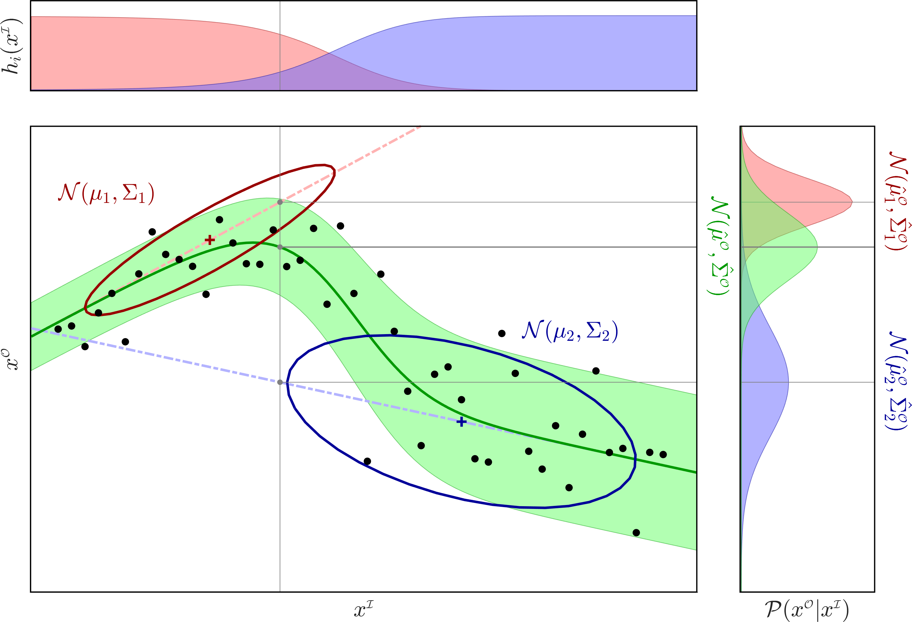
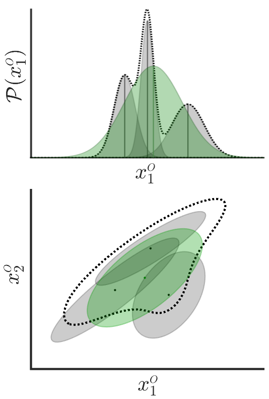
Figure 3: Left: Gaussian mixture regression (GMR) for 1D input $x^{\scriptscriptstyle{I}}$ and 1D output $x^{\scriptscriptstyle{O}}$, with a GMM composed of two Gaussians. Right: Gaussian that best approximates a mixture of three Gaussians. The multimodal distributions in dashed line depict the probability density functions for the mixtures of three Gaussians in gray color (examples in 1D and 2D are depicted). The Gaussians in green color approximate these multimodal distributions.

Gaussian mixture regression (GMR) is a another popular technique for time series and motion representations Ghahramani and Jordan (1994); Calinon and Lee (2019). It relies on linear transformation and conditioning properties of multivariate Gaussian distributions. GMR provides a synthesis mechanism to compute output distributions with a computation time independent of the number of datapoints used to train the model. A characteristic of GMR is that it does not model the regression function directly. Instead, it first models the joint probability density of the data in the form of a Gaussian mixture model (GMM). It can then compute the regression function from the learned joint density model, resulting in very fast computation of a conditional distribution.

In GMR, both input and output variables can be multidimensional. Any subset of input–output dimensions can be selected, which can change, if required, at each time step. Thus, any combination of input–output mappings can be considered, where expectations on the remaining dimensions are computed as a multivariate distribution. In the following, we will denote the block decomposition of a datapoint $\bm{x}_{t}\in\mathbb{R}^{D}$ at time step $t$, and the center $\bm{\mu}_{k}$ and covariance $\bm{\Sigma}_{k}$ of the $k$-th Gaussian in the GMM as

$$\bm{x}_{t}=\begin{bmatrix}\bm{x}^{\scriptscriptstyle{I}}_{t}\\ \bm{x}^{\scriptscriptstyle{O}}_{t}\end{bmatrix}\;,\quad\bm{\mu}_{k}=\begin{bmatrix}\bm{\mu}^{\scriptscriptstyle{I}}_{k}\\ \bm{\mu}^{\scriptscriptstyle{O}}_{k}\end{bmatrix}\;,\quad\bm{\Sigma}_{k}=\begin{bmatrix}\bm{\Sigma}^{\scriptscriptstyle{I}}_{k}\;\bm{\Sigma}^{\scriptscriptstyle{IO}}_{k}\\ \bm{\Sigma}^{\scriptscriptstyle{OI}}_{k}\bm{\Sigma}^{\scriptscriptstyle{O}}_{k}\end{bmatrix}.$$ (6)

We first consider the example of time-based trajectories by using $\bm{x}^{\scriptscriptstyle{I}}_{t}$ as a time variables. At each time step $t$, $\mathcal{P}(\bm{x}^{\scriptscriptstyle{O}}_{t}|\bm{x}^{\scriptscriptstyle{I}}_{t})$ can be computed as the multimodal conditional distribution

$$\mathcal{P}(\bm{x}^{\scriptscriptstyle{O}}_{t}|\bm{x}^{\scriptscriptstyle{I}}_{t}) \;=\;\sum_{k=1}^{K}h_{k}(\bm{x}^{\scriptscriptstyle{I}}_{t})\;\mathcal{N}\!\left(\bm{\hat{\mu}}^{\scriptscriptstyle{O}}_{k}(\bm{x}^{\scriptscriptstyle{I}}_{t}),\bm{\hat{\Sigma}}^{\scriptscriptstyle{O}}_{k}\right),$$ (7)

$$\mathrm{with}\quad\bm{\hat{\mu}}^{\scriptscriptstyle{O}}_{k}(\bm{x}^{\scriptscriptstyle{I}}_{t}) \;=\;\bm{\mu}^{\scriptscriptstyle{O}}_{k}+\bm{\Sigma}^{\scriptscriptstyle{OI}}_{k}{\bm{\Sigma}^{\scriptscriptstyle{I}}_{k}}^{-1}(\bm{x}^{\scriptscriptstyle{I}}_{t}-\bm{\mu}^{\scriptscriptstyle{I}}_{k})\;,$$

$$\bm{\hat{\Sigma}}^{\scriptscriptstyle{O}}_{k} \;=\;\bm{\Sigma}^{\scriptscriptstyle{O}}_{k}-\bm{\Sigma}^{\scriptscriptstyle{OI}}_{k}{\bm{\Sigma}^{\scriptscriptstyle{I}}_{k}}^{-1}\bm{\Sigma}^{\scriptscriptstyle{IO}}_{k},$$

$$\mathrm{and}\quad h_{k}(\bm{x}^{\scriptscriptstyle{I}}_{t}) \;=\;\frac{\pi_{k}\;\mathcal{N}(\bm{x}^{\scriptscriptstyle{I}}_{t}|\;\bm{\mu}^{\scriptscriptstyle{I}}_{k},\bm{\Sigma}^{\scriptscriptstyle{I}}_{k})}{\sum_{i=1}^{K}\pi_{i}\;\mathcal{N}(\bm{x}^{\scriptscriptstyle{I}}_{t}|\;\bm{\mu}^{\scriptscriptstyle{I}}_{i},\bm{\Sigma}^{\scriptscriptstyle{I}}_{i})},$$

computed with

$$\mathcal{N}(\bm{x}^{\scriptscriptstyle{I}}_{t}|\;\bm{\mu}^{\scriptscriptstyle{I}}_{k},\bm{\Sigma}^{\scriptscriptstyle{I}}_{k})=(2\pi)^{-\frac{D}{2}}{|\bm{\Sigma}^{\scriptscriptstyle{I}}_{k}|}^{-\frac{1}{2}}\exp\Big{(}\!-\frac{1}{2}{(\bm{x}^{\scriptscriptstyle{I}}_{t}-\bm{\mu}^{\scriptscriptstyle{I}}_{k})}^{{\scriptscriptstyle\top}}{\bm{\Sigma}^{\scriptscriptstyle{I}}_{k}}^{-1}(\bm{x}^{\scriptscriptstyle{I}}_{t}-\bm{\mu}^{\scriptscriptstyle{I}}_{k})\!\Big{)}.$$

When a unimodal output distribution is required, the law of total mean and variance (see Fig. 3-right) can be used to approximate the distribution with the Gaussian

$$\mathcal{P}(\bm{x}_{t}^{\scriptscriptstyle{O}}|\bm{x}_{t}^{\scriptscriptstyle{I}}) =\mathcal{N}\Big{(}\bm{x}_{t}^{\scriptscriptstyle{O}}|\;\bm{\hat{\mu}}{}^{\scriptscriptstyle{O}}\!(\bm{x}_{t}^{\scriptscriptstyle{I}}),\bm{\hat{\Sigma}}{}^{\scriptscriptstyle{O}}\!(\bm{x}_{t}^{\scriptscriptstyle{I}})\Big{)},$$ (8)

$$\mathrm{with}\quad\bm{\hat{\mu}}{}^{\scriptscriptstyle{O}}\!(\bm{x}_{t}^{\scriptscriptstyle{I}}) =\sum_{k=1}^{K}\!h_{k}(\bm{x}_{t}^{\scriptscriptstyle{I}})\;\bm{\hat{\mu}}_{k}^{\scriptscriptstyle{O}}\!(\bm{x}_{t}^{\scriptscriptstyle{I}}),$$

$$\mathrm{and}\quad\bm{\hat{\Sigma}}{}^{\scriptscriptstyle{O}}\!(\bm{x}_{t}^{\scriptscriptstyle{I}}) =\sum_{k=1}^{K}\!h_{k}(\bm{x}^{\scriptscriptstyle{I}}_{t})\Big{(}\bm{\hat{\Sigma}}_{k}^{\scriptscriptstyle{O}}\!+\!\bm{\hat{\mu}}_{k}^{\scriptscriptstyle{O}}\!(\bm{x}_{t}^{\scriptscriptstyle{I}})\;{\bm{\hat{\mu}}_{k}^{\scriptscriptstyle{O}}\!(\bm{x}_{t}^{\scriptscriptstyle{I}})}^{\scriptscriptstyle\top}\Big{)}-\bm{\hat{\mu}}{}^{\scriptscriptstyle{O}}\!(\bm{x}_{t}^{\scriptscriptstyle{I}})\,{\bm{\hat{\mu}}{}^{\scriptscriptstyle{O}}\!(\bm{x}_{t}^{\scriptscriptstyle{I}})\phantom{}}^{\scriptscriptstyle\top}.$$

Figure 3 presents an example of GMR with 1D input and 1D output. With the GMR representation, LWR corresponds to a GMM with diagonal covariances. Expressing LWR in the more general form of GMR has several advantages: (1) it allows the encoding of local correlations between the motion variables by extending the diagonal covariances to full covariances; (2) it provides a principled approach to estimate the parameters of the RBFs, similar to a GMM parameters fitting problem; (3) it often allows a significant reduction of the number of RBFs, because the position and spread of each RBF are also estimated; and (4) the (online) estimation of the mixture model parameters and the model selection problem (automatically estimating the number of basis functions) can readily exploit techniques compatible with GMM (Bayesian nonparametrics with Dirichlet processes, spectral clustering, small variance asymptotics, expectation-maximization procedures, etc.).

Another approach to encode and synthesize a movement is to rely on time-invariant autonomous systems. GMR can also be employed in this context to retrieve an autonomous system $\mathcal{P}(\bm{\dot{x}}|\bm{x})$ from the joint distribution $\mathcal{P}(\bm{x},\bm{\dot{x}})$ encoded in a GMM, where $\bm{x}$ and $\bm{\dot{x}}$ are position and velocity, respectively (see Hersch et al. (2008) for details). Similarly, it can be used in an autoregressive context by retrieving $\mathcal{P}(\bm{x}_{t}|\bm{x}_{t-1},\bm{x}_{t-2},\ldots,\bm{x}_{t-T})$ at each time step $t$, from the joint encoding of the positions on a time window of size $T$.

Practical applications of GMR include the analysis of speech signals Toda et al. (2007); Hueber and Bailly (2016), electromyography signals Jaquier and Calinon (2017), vision and MoCap data Tian et al. (2013), and cancer prognosis Falk et al. (2006). A Matlab code example demo_GMR01.m can be found in pbd (Accessed: 2019/04/18).

2.2 Bernstein basis functions

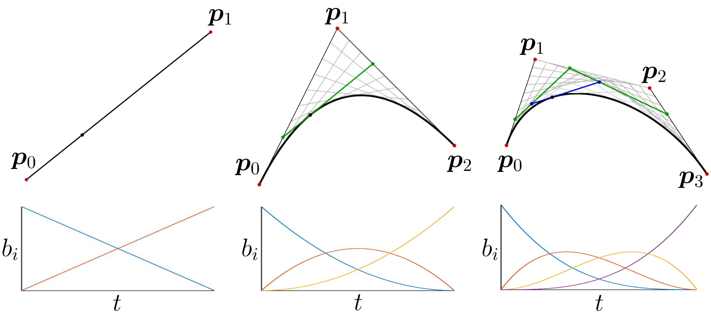
Figure 4: Linear (left), quadratic (center) and cubic (right) Bézier curves constructed as a weighted superposition of Bernstein basis functions.

Bézier curves are well-known representations of trajectories Farouki (2012). Their underlying representation is a superposition of basis functions, which is overlooked in many applications. For $0\leqslant t\leqslant 1$, a linear Bézier curve is the line traced by the function $\bm{x}_{\scriptscriptstyle{\bm{p}_{0},\bm{p}_{1}}}(t)$, from $\bm{p}_{0}$ to $\bm{p}_{1}$,

$$\bm{x}_{\scriptscriptstyle{\bm{p}_{0},\bm{p}_{1}}}(t) =(1-t)\,\bm{p}_{0}+t\,\bm{p}_{1}.$$ (9)

For $0\leqslant t\leqslant 1$, a quadratic Bézier curve is the path traced by the function

$$\bm{x}_{\scriptscriptstyle{\bm{p}_{0},\bm{p}_{1},\bm{p}_{2}}}(t) =(1-t)\;\bm{x}_{\scriptscriptstyle{\bm{p}_{0},\bm{p}_{1}}}(t)+t\;\bm{x}_{\scriptscriptstyle{\bm{p}_{1},\bm{p}_{2}}}(t)$$

$$=(1-t)\Big{(}(1-t)\bm{p}_{0}+t\,\bm{p}_{1}\Big{)}+t\Big{(}(1-t)\bm{p}_{1}+t\,\bm{p}_{2}\Big{)}$$

$$=(1-t)^{2}\bm{p}_{0}+2(1-t)t\,\bm{p}_{1}+t^{2}\bm{p}_{2}.$$ (10)

For $0\leqslant t\leqslant 1$, a cubic Bézier curve is the path traced by the function

$$\bm{x}_{\scriptscriptstyle{\bm{p}_{0},\bm{p}_{1},\bm{p}_{2},\bm{p}_{3}}}(t) =(1-t)\;\bm{x}_{\scriptscriptstyle{\bm{p}_{0},\bm{p}_{1},\bm{p}_{2}}}(t)+t\;\bm{x}_{\scriptscriptstyle{\bm{p}_{1},\bm{p}_{2},\bm{p}_{3}}}(t)$$

$$=(1-t)^{3}\bm{p}_{0}+3(1-t)^{2}t\bm{p}_{1}+3(1-t)t^{2}\bm{p}_{2}+t^{3}\bm{p}_{3}.$$ (11)

For $0\leqslant t\leqslant 1$, a recursive definition for a Bézier curve of degree $n$ can be expressed as a linear interpolation of a pair of corresponding points in two Bézier curves of degree $n-1$, namely

$$\bm{x}(t)=\sum_{i=0}^{n}b_{i,n}(t)\,\bm{p}_{i},\quad\mathrm{with}\quad b_{i,n}(t)=\frac{n!}{i!(n-i)!}\;(1-t)^{n-i}\;t^{i},$$ (12)

with $b_{i,n}(t)$ the Bernstein basis polynomials of degree n, where $\frac{n!}{i!(n-i)!}$ are binomial coefficients, which can also be noted as $\binom{n}{i}$.

Figure 4 illustrates the construction of Bézier curves of different orders. Practical applications are diverse but include most notably trajectories in computer graphics Farouki (2012) and path planning Egerstedt and Martin (2010). A Matlab code example demo_Bezier01.m can be found in pbd (Accessed: 2019/04/18).

2.3 Fourier basis functions

In this section, we will adopt a notation to make links with the superposition of basis functions seen in Fig. 1. By starting with the unidimensional case, we will consider a signal $g(x)$ varying along a variable $x$, where $x$ will be used as a generic variable that can for example be a time variable as in the example of Fig. 1, or the coordinates of a pixel in an image. The signal $g(x)$ can be approximated as a weighted superposition of basis functions with

$$g(x) =\sum_{k=-K\!+\!1}^{K\!-\!1}w_{k}\,\phi_{k}(x)$$

$$=\bm{w}^{\scriptscriptstyle\top}\bm{\phi}(x),$$

where $\bm{w}$ and $\bm{\phi}(x)$ are vectors formed with the elements of $w_{k}$ and $\phi_{k}(x)$, respectively. $w_{k}$ and $\phi_{k}(x)$ denote the coefficients and basis functions of the Fourier series, with

$$\phi_{k}(x) =\frac{1}{L}\exp\!\left(-i\frac{2\pi kx}{L}\right)$$

$$=\frac{1}{L}\Bigg{(}\!\cos\!\left(\frac{2\pi kx}{L}\right)-i\,\sin\!\left(\frac{2\pi kx}{L}\right)\!\Bigg{)},\;\forall k\!\in\![-K\!+\!1,\ldots,K\!-\!1],$$ (13)

with $i$ the imaginary unit of a complex number ($i^{2}=-1$).

In time series encoding, the use of Fourier basis functions provides useful connections between the spatial domain and the frequency domain. In the context of Gaussian mixture models, several Fourier series properties can be exploited, notably regarding zero-centered Gaussians, shift, symmetry, and linear combination. These properties are reported in Table 1 for the 1D case.

Table 1: Fourier series properties (1D case).

Symmetry property:
If $g(x)$ is real and even, $\phi_{k}(x)$ in (13) is also real and even, simplifying to $\phi_{k}(x)=\frac{1}{L}\cos\!\left(\frac{2\pi kx}{L}\right)$, which then, in practice, only needs an evaluation on the range $k\!\in\![0,\ldots,K\!-\!1]$, as the basis functions are even. We then have $g(x)=w_{0}+\sum_{k=1}^{K\!-\!1}w_{k}\,2\cos\!\left(\frac{2\pi kx}{L}\right)$, by exploiting $\cos(0)\!=\!1$.
Shift property:
If $w_{k}$ are the Fourier series coefficients of a function $g(x)$, $\exp(-i\frac{2\pi k\mu}{L})w_{k}$ are the Fourier coefficients of $g(x-\mu)$.
Combination property:
If $w_{k,1}$ (resp. $w_{k,2}$) are the Fourier series coefficients of a function $g_{1}(x)$ (resp. $g_{2}(x)$), then $\alpha_{1}w_{k,1}+\alpha_{2}w_{k,2}$ are the Fourier coefficients of $\alpha_{1}g_{1}(x)+\alpha_{2}g_{2}(x)$.
Gaussian property:
If $g_{0}(x)=\mathcal{N}(x\,|\,0,\sigma^{2})=(2\pi\sigma^{2})^{-\frac{1}{2}}\exp(-\frac{x^{2}}{2\sigma^{2}})$ is mirrored to create a real and even periodic function $g(x)$ of period $L\gg\sigma$ (implementation details will follow), the corresponding Fourier series coefficients are of the form $w_{k}=\exp(-\frac{2\pi^{2}k^{2}\sigma^{2}}{L^{2}})$.

Well-known applications of Fourier basis functions in the context of time series include speech processing Toda et al. (2007); Hueber and Bailly (2016) and the analysis of periodic motions such as gaits Antonsson and Mann (1985). Such decompositions also have a wider scope of applications, as illustrated next with ergodic control.

2.4 Ergodic control

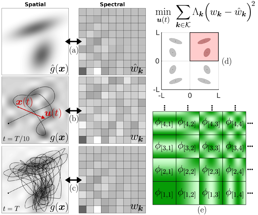
Figure 5: 2D ergodic control problem. (a) shows the spatial distribution $\hat{g}(\bm{x})$ that the agent has to explore, encoded here as a mixture of two Gaussians (gray colormap in left graph). The right graphs show the corresponding Fourier series coefficients $\hat{w}_{\bm{k}}$ in the frequency domain ($K=9$ coefficients per dimension), which can be computed analytically by exploiting the shift, symmetry and linear combination properties of Gaussians. (b) shows the evolution of the reconstructed spatial distribution $g(\bm{x})$ (left graph) and the computation of the next control command $\bm{u}$ (red arrow) after $T/10$ iterations. The corresponding Fourier series coefficients $w_{\bm{k}}$ are shown in the right graph. (c) shows that after $T$ iterations, the agent covers the space in proportion to the desired spatial distribution, with a good match of coefficients in the frequency domain (we can see that $\hat{w}_{\bm{k}}$ and $w_{\bm{k}}$ are nearly the same). (d) shows how a periodic signal $\hat{g}(\bm{x})$ (with range $[-L/2,L/2]$ for each dimension) can be constructed from the original mixture of two Gaussians $\hat{g}_{0}(\bm{x})$ (red area). The constructed signal $\hat{g}(\bm{x})$ is composed of eight Gaussians in this 2D example (mirroring the Gaussians along horizontal and vertical axes to construct an even signal of period $L$). (e) depicts the first few basis functions of the Fourier series (for the first four coefficients in each dimension), represented as a 2D colormap corresponding to periodic signals of different frequencies along two axes.

In ergodic control, the aim is to find a series of control commands $\bm{u}(t)$ so that the retrieved trajectory $\bm{x}(t)\in\mathbb{R}^{D}$ covers a bounded space $\mathcal{X}$ in proportion of a desired spatial distribution $\hat{g}(\bm{x})$, see Fig. 5-(a). As proposed in Mathew and Mezic (2011), this can be achieved by defining a metric in the spectral domain, by decomposing in Fourier series coefficients both the desired spatial distribution $\hat{g}(\bm{x})$ and the (partially) retrieved trajectory $\bm{x}(t)$. The goal of ergodic control is to minimize

$$\epsilon =\frac{1}{2}\sum_{{\bm{k}}\in\mathcal{K}}\Lambda_{\bm{k}}\Big{(}w_{\bm{k}}-\hat{w}_{\bm{k}}\Big{)}^{\!2}$$ (14)

$$=\frac{1}{2}{\Big{(}\bm{w}-\bm{\hat{w}}\Big{)}}^{\!{\scriptscriptstyle\top}}\bm{\Lambda}\,\Big{(}\bm{w}-\bm{\hat{w}}\Big{)},$$ (15)

where $\Lambda_{\bm{k}}$ are weights, $\hat{w}_{\bm{k}}$ are the Fourier series coefficients of $\hat{g}(\bm{x})$, and $w_{\bm{k}}$ are the Fourier series coefficients along the trajectory $\bm{x}(t)$. $\mathcal{K}$ is a set of index vectors in $\mathbb{N}^{D}$ covering the $D$-dimensional array $\bm{k}=\bm{r}\times\bm{r}\times\cdots\times\bm{r}$, with $\bm{r}=[0,1,\ldots,K\!-\!1]$ and $K$ the resolution of the array. $\bm{w}\in\mathbb{R}^{K^{D}}$ and $\bm{\hat{w}}\in\mathbb{R}^{K^{D}}$ are vectors composed of elements $w_{\bm{k}}$ and $\hat{w}_{\bm{k}}$, respectively. $\bm{\Lambda}\in\mathbb{R}^{K^{D}\times K^{D}}$ is a diagonal weighting matrix with elements $\Lambda_{\bm{k}}$. In (14), the weights

$$\Lambda_{\bm{k}}=\left(1+\|\bm{k}\|^{2}\right)^{\!-\frac{D+1}{2}}$$ (16)

assign more importance on matching low frequency components (related to a metric for Sobolev spaces of negative order). The Fourier series coefficients $w_{\bm{k}}$ along a trajectory $\bm{x}(t)$ of continuous duration $t$ are defined as

$$w_{\bm{k}}=\frac{1}{t}\int_{\tau=0}^{t}\phi_{\bm{k}}\big{(}\bm{x}(\tau)\big{)}\;d\tau,$$ (17)

whose discretized version can be computed recursively at each discrete time step $t$ to build

$$w_{\bm{k}}=\frac{1}{t}\sum_{s=1}^{t}\phi_{\bm{k}}(\bm{x}_{s}),$$ (18)

or equivalently in vector form $\bm{w}=\frac{1}{t}\sum_{s=1}^{t}\bm{\phi}(\bm{x}_{s})$.

For a spatial signal $\bm{x}\in\mathbb{R}^{D}$, where $x_{d}$ is on the interval $[-\frac{L}{2},\frac{L}{2}]$ of period $L$, $\forall d\!\in\!\{1,\ldots,D\}$, the basis functions of the Fourier series with complex exponential functions are defined as (see Fig. 5-(e))

$$\phi_{\bm{k}}(\bm{x}) =\frac{1}{L^{D}}\prod_{d=1}^{D}\exp\!\left(-i\frac{2\pi k_{d}x_{d}}{L}\right)$$

$$=\frac{1}{L^{D}}\prod_{d=1}^{D}\cos\!\left(\frac{2\pi k_{d}x_{d}}{L}\right)-i\,\sin\!\left(\frac{2\pi k_{d}x_{d}}{L}\right),\quad\forall\bm{k}\!\in\!\mathcal{K}.$$ (19)

Computation of Fourier series coefficients $\hat{w}_{\bm{k}}$ for a spatial distribution represented as a Gaussian mixture model

We consider a desired spatial distribution $\hat{g}_{0}(\bm{x})$ represented as a mixture of $J$ Gaussians with centers $\bm{\mu}_{j}$, covariance matrices $\bm{\Sigma}_{j}$, and mixing coefficients $\alpha_{j}$ (with $\sum_{j=1}^{J}\alpha_{j}=1$ and $\alpha_{j}\geqslant 0$),

$$\hat{g}_{0}(\bm{x}) =\sum_{j=1}^{J}\alpha_{j}\,\mathcal{N}\big{(}\bm{x}\,|\,\bm{\mu}_{j},\bm{\Sigma}_{j}\big{)}$$ (20)

$$=\sum_{j=1}^{J}\alpha_{j}\,(2\pi)^{-\!\frac{D}{2}}\,{|\bm{\Sigma}_{j}|}^{-\!\frac{1}{2}}\,\exp\!\Big{(}\!-\!\frac{1}{2}{(\bm{x}\!-\!\bm{\mu}_{j})}^{{\scriptscriptstyle\top}}\bm{\Sigma}_{j}^{-1}(\bm{x}\!-\!\bm{\mu}_{j})\!\Big{)},$$

with each dimension on the interval $[0,\frac{L}{2}]$. $\hat{g}_{0}(\bm{x})$ is extended to a periodized function by constructing an even function on the interval $\mathcal{X}$, where each dimension $x_{d}$ is on the interval $\mathcal{X}\!=\![-\frac{L}{2},\frac{L}{2}]$ of period $L$. This is achieved with mirror symmetries of the Gaussians around all zero axes, see Fig. 5-(d). The resulting spatial distribution can be expressed as a mixture of $2^{D}J$ Gaussians

$$\hat{g}(\bm{x})=\sum_{j=1}^{J}\sum_{m=1}^{2^{D}}\frac{\alpha_{j}}{2^{D}}\;\mathcal{N}\big{(}\bm{x}\,\big{|}\,\bm{A}_{m}\bm{\mu}_{j},\bm{A}_{m}\bm{\Sigma}_{j}\bm{A}_{m}^{\scriptscriptstyle\top}\big{)},$$ (21)

with linear transformation matrices $\bm{A}_{m}$. By exploiting the symmetry, shift and Gaussian properties presented in Section 2.3, the Fourier series coefficients $\hat{w}_{\bm{k}}$ can be analytically computed as

$$\hat{w}_{\bm{k}} =\int_{\bm{x}\in\mathcal{X}}\hat{g}(\bm{x})\;\phi_{\bm{k}}(\bm{x})\;\text{d}\bm{x}$$

$$=\frac{1}{L^{D}}\sum_{j=1}^{J}\sum_{m=1}^{2^{D}}\frac{\alpha_{j}}{2^{D}}\exp\!\left(-i\frac{2\pi\bm{k}^{{\scriptscriptstyle\top}}\bm{A}_{m}\bm{\mu}_{j}}{L}\right)\exp\!\left(-\frac{2\pi^{2}\bm{k}^{{\scriptscriptstyle\top}}\bm{A}_{m}\bm{\Sigma}_{j}\bm{A}_{m}^{\scriptscriptstyle\top}\bm{k}}{L^{2}}\right)$$

$$=\frac{1}{L^{D}}\sum_{j=1}^{J}\sum_{m=1}^{2^{D-1}}\frac{\alpha_{j}}{2^{D-1}}\cos\!\left(\frac{2\pi\bm{k}^{{\scriptscriptstyle\top}}\bm{A}_{m}\bm{\mu}_{j}}{L}\right)\exp\!\left(-\frac{2\pi^{2}\bm{k}^{{\scriptscriptstyle\top}}\bm{A}_{m}\bm{\Sigma}_{j}\bm{A}_{m}^{\scriptscriptstyle\top}\bm{k}}{L^{2}}\right).$$ (22)

With this mirroring, we can see that $\hat{w}_{\bm{k}}$ are real and even, where an evaluation over $\bm{k}\!\in\!\mathcal{K}$, $j\!\in\!\{1,2,\ldots,J\}$ and $m\!\in\!\{1,2,\ldots,2^{D-1}\}$ in (22) is sufficient to fully characterize the signal.

Controller for a spatial distribution represented as a Gaussian mixture model

In Mathew and Mezic (2011), ergodic control is set as the constrained problem of computing a control command $\bm{\hat{u}}(t)$ at each time step $t$ with

$$\bm{\hat{u}}(t)=\arg\min_{\bm{u}(t)}\;\epsilon\big{(}\bm{x}(t\!+\!\Delta t)\big{)},\quad\text{s.t.}\quad\bm{\dot{x}}(t)=f\big{(}\bm{x}(t),\bm{u}(t)\big{)},\quad\|\bm{u}(t)\|\leqslant u^{\max},$$ (23)

where the simple system $\bm{\dot{x}}(t)=\bm{u}(t)$ is considered (control with velocity commands), and where the error term is approximated with the Taylor series

$$\epsilon\big{(}\bm{x}(t\!+\!\Delta t)\big{)}\;\approx\;\epsilon\big{(}\bm{x}(t)\big{)}\;+\;\dot{\epsilon}\big{(}\bm{x}(t)\big{)}\Delta t\;+\;\frac{1}{2}\ddot{\epsilon}\big{(}\bm{x}(t)\big{)}{\Delta t}^{2}.$$ (24)

By using (14), (17), (19) and the chain rule $\frac{\partial f}{\partial t}=\frac{\partial f}{\partial\bm{x}}\frac{\partial\bm{x}}{\partial t}$, the Taylor series is composed of the control term $\bm{u}(t)$ and $\nabla_{\!\!\bm{x}}\phi_{\bm{k}}\big{(}\bm{x}(t)\big{)}\in\mathbb{R}^{1\times D}$, the gradient of $\phi_{\bm{k}}\big{(}\bm{x}(t)\big{)}$ with respect to $\bm{x}(t)$. Solving the constrained objective in (23) then results in the analytical solution (see Mathew and Mezic (2011) for the complete derivation)

$$\bm{u}=\bm{\tilde{u}}(t)\frac{u^{\max}}{\|\bm{\tilde{u}}(t)\|},\quad\mathrm{with}\quad\bm{\tilde{u}} =-\sum_{{\bm{k}}\in\mathcal{K}}\Lambda_{\bm{k}}\big{(}w_{\bm{k}}-\hat{w}_{\bm{k}}\big{)}{\nabla_{\!\!\bm{x}}\phi_{\bm{k}}\big{(}\bm{x}(t)\big{)}}^{\scriptscriptstyle\top}$$

$$=-\bm{\nabla}_{\!\!\bm{x}}\bm{\phi}\big{(}\bm{x}(t)\big{)}\;\bm{\Lambda}\,\big{(}\bm{w}-\bm{\hat{w}}\big{)},$$ (25)

where $\bm{\nabla}_{\!\!\bm{x}}\bm{\phi}\big{(}\bm{x}(t)\big{)}\in\mathbb{R}^{D\times K^{D}}$ is a concatenation of the vectors $\nabla_{\!\!\bm{x}}\phi_{\bm{k}}\big{(}\bm{x}(t)\big{)}$. Figure 5 shows a 2D example of ergodic control to create a motion approximating the distribution given by a mixture of two Gaussians. A remarkable characteristic of such approach is that the controller produces natural exploration behaviors (see Fig. 5-(c)) without relying on stochastic noise in the formulation. In the limit case, if the distribution $g(\bm{x})$ is a single Gaussian with a very small isotropic covariance, the controller results in a standard tracking behavior.

Examples of application include surveillance with multi-agent systems Mathew and Mezic (2011), active shape estimation Abraham et al. (2017), and localization for fish-like robots Miller et al. (2016). A Matlab code example demo_ergodicControl_2D01.m can be found in pbd (Accessed: 2019/04/18).

3 Probabilistic movement primitives

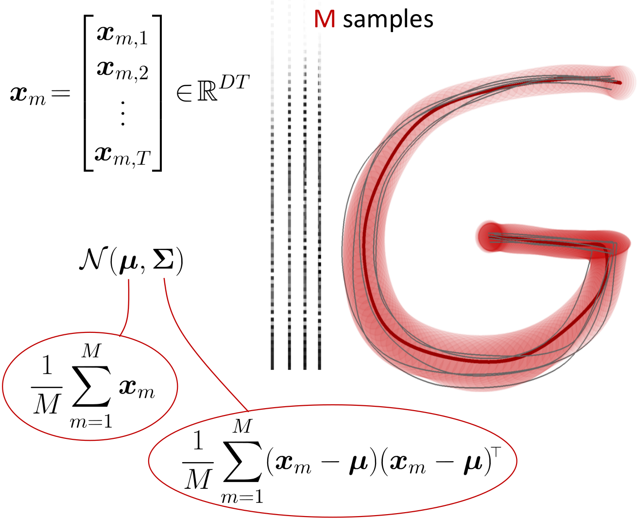
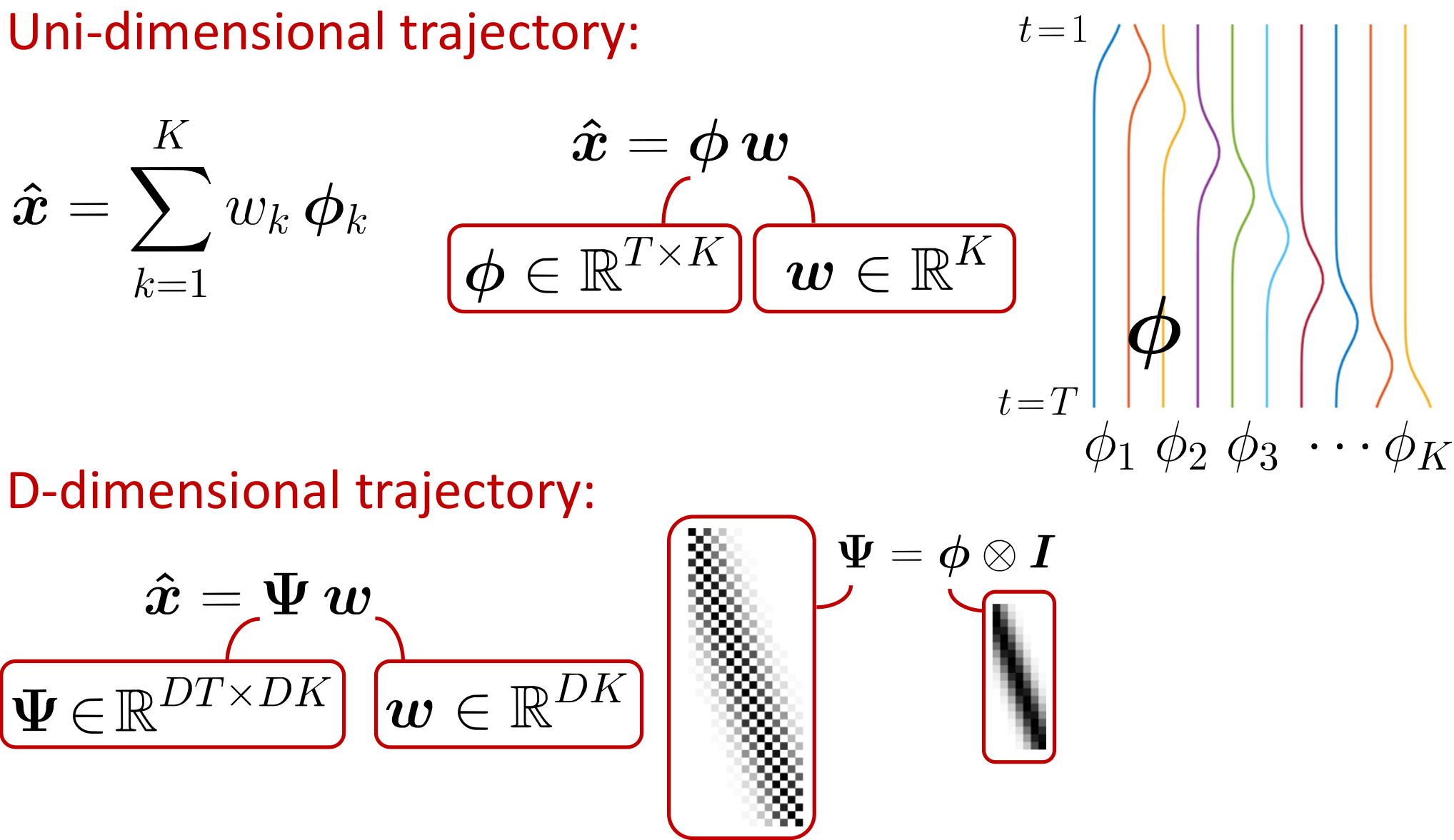
Figure 6: Left: Raw trajectory distribution as a Gaussian of size $DT$ by organizing each of the $M$ samples as a trajectory vector, where each trajectory has $T$ time steps and each point has $D$ dimensions ($T=100$ and $D=2$ in this example). Right: Trajectory distribution encoded with probabilistic movement primitives (superposition of $K$ basis functions). The right part of the figure depicts the linear mapping functions $\bm{\phi}$ and $\bm{\Psi}$ created by a decomposition with radial basis functions.

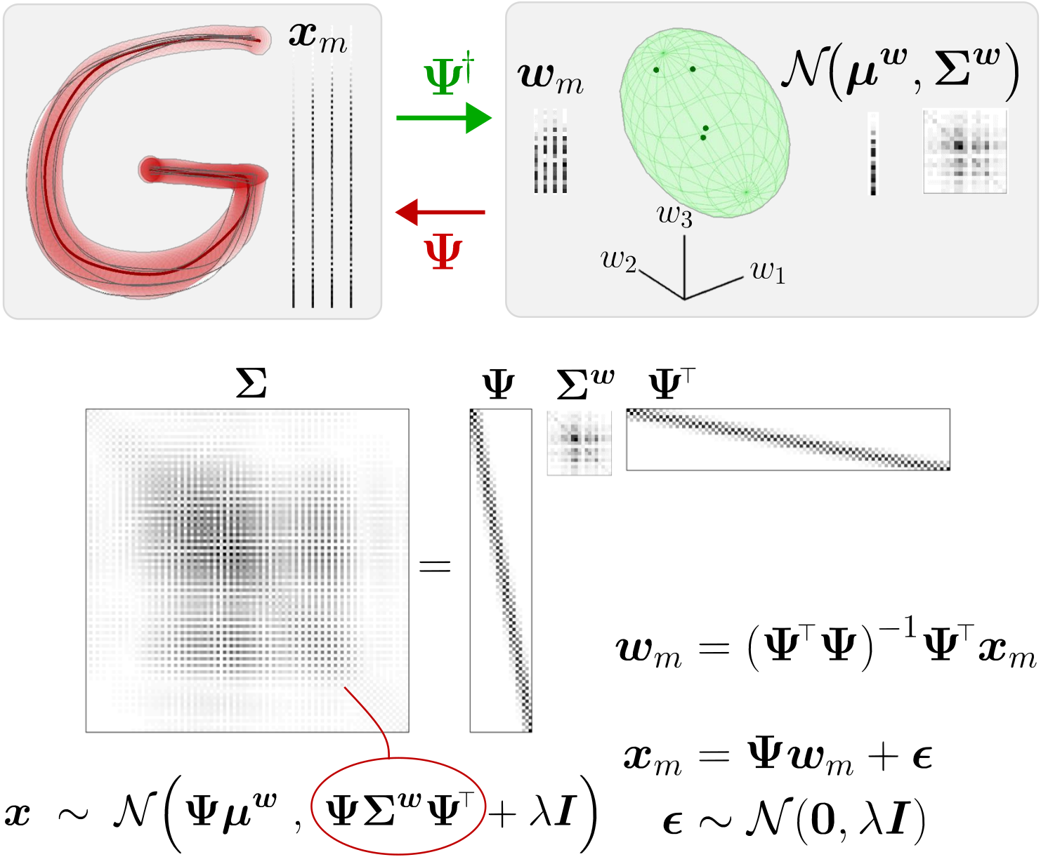
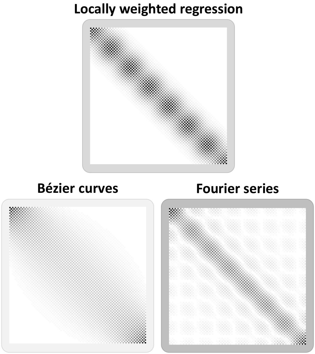
Figure 7: Left: Illustration of probabilistic movement primitives as a linear mapping between the original space of trajectories and a subspace of reduced dimensionality. After projecting each trajectory sample in this subspace (with linear map $\bm{\Psi}^{\dagger}$ computed as the pseudoinverse of $\bm{\Psi}$), a Gaussian is evaluated, which is then projected back to the original trajectory space by exploiting the linear transformation property of multivariate Gaussians (with linear map $\bm{\Psi}$). Such decomposition results in a low rank structure of the covariance matrix, which is depicted in the bottom part of the figure. Right: Representation of the covariance matrix $\bm{\Psi}\bm{\Psi}^{\scriptscriptstyle\top}$ for various basis functions, all showing some form of sparsity.

The representation of time series as a superposition of basis functions can also be exploited to construct trajectory distributions. Representing a collection of trajectories in the form of a multivariate distribution has several advantages. First, new trajectories can be stochastically generated. Then, the conditional probability property (see (7)) can be exploited to generate trajectories passing through via-points (including starting and/or ending points). This is simply achieved by specifying as inputs $\bm{x}^{\scriptscriptstyle{I}}$ in (7) the datapoints that the system needs to pass through (with corresponding dimensions in the hyperdimensional vector) and by retrieving as output $\bm{x}^{\scriptscriptstyle{O}}$ the remaining parts of the trajectory.

A naive approach to represent a collection of $M$ trajectories in a probabilistic form is to reorganize each trajectory as a hyperdimensional datapoint $\bm{x}_{m}\!=\!{[\bm{x}_{1}^{\scriptscriptstyle\top},\bm{x}_{2}^{\scriptscriptstyle\top},\ldots,\bm{x}_{T}^{\scriptscriptstyle\top}]}^{\scriptscriptstyle\top}\!\in\!\mathbb{R}^{DT}$, and fitting a Gaussian $\mathcal{N}(\bm{\mu}^{\bm{x}},\bm{\Sigma}^{\bm{x}})$ to these datapoints, see Fig. 6-left. Since the dimension $DT$ might be much larger than the number of datapoints $M$, a potential solution to this issue could be to consider an eigendecomposition of the covariance (ordered by decreasing eigenvalues)

$$\bm{\Sigma}^{\bm{x}}=\bm{V}\bm{D}\bm{V}^{\scriptscriptstyle\top}=\sum_{j=1}^{DT}\lambda^{2}_{j}\,\bm{v}_{j}\,\bm{v}_{j}^{\scriptscriptstyle\top},$$ (26)

with $\bm{V}\!=\![\bm{v}_{1},\bm{v}_{2},\ldots,\bm{v}_{DT}]$ and $\bm{D}\!=\!\mathrm{diag}(\lambda^{2}_{1},\lambda^{2}_{2},\ldots,\lambda^{2}_{DT})$. This can be exploited to project the data in a subspace of reduced dimensionality through principal component analysis. By keeping the first $DK$ components, such approach provides a Gaussian distribution of the trajectories with the structure $\mathcal{N}(\bm{\Psi}\bm{\mu}^{\bm{w}},\bm{\Psi}\bm{\Psi}^{\scriptscriptstyle\top})$, where $\bm{\Psi}\!=\![\bm{v}_{1}\lambda_{1},\,\bm{v}_{2}\lambda_{2},\,\ldots,\,\bm{v}_{DK}\lambda_{DK}]$.

The ProMP (probabilistic movement primitive) model proposed in Paraschos et al. (2013) also encodes the trajectory distribution in a subspace of reduced dimensionality, but provides a RBF structure to this decomposition instead of the eigendecomposition as in the above. It assumes that each sample trajectory $m\!\in\!\{1,\ldots,M\}$ can be approximated by a weighted sum of $K$ normalized RBFs with

$$\bm{x}_{m}=\bm{\Psi}\bm{w}_{m}+\bm{\epsilon},\quad\mathrm{where}\quad\bm{\epsilon}\sim\mathcal{N}(\bm{0},\sigma^{2}\bm{I}),$$ (27)

and basis functions organized as

$$\bm{\Psi}=\bm{\phi}\otimes\bm{I}=\left[\begin{matrix}\bm{I}\phi_{1}(t_{1})&\bm{I}\phi_{2}(t_{1})&\cdots&\bm{I}\phi_{K}(t_{1})\\ \bm{I}\phi_{1}(t_{2})&\bm{I}\phi_{2}(t_{2})&\cdots&\bm{I}\phi_{K}(t_{2})\\ \vdots&\vdots&\ddots&\vdots\\ \bm{I}\phi_{1}(t_{T})&\bm{I}\phi_{2}(t_{T})&\cdots&\bm{I}\phi_{K}(t_{T})\end{matrix}\right],$$ (28)

with $\bm{\Psi}\!\in\!\mathbb{R}^{DT\times DK}$, identity matrix $\bm{I}\!\in\!\mathbb{R}^{D\!\times\!D}$, and $\otimes$ the Kronecker product operator. A vector $\bm{w}_{m}\!\in\!\mathbb{R}^{DK}$ can be estimated for each of the $M$ sample trajectories by the least squares estimate

$$\bm{w}_{m}={(\bm{\Psi}^{\scriptscriptstyle\top}\bm{\Psi})}^{-1}\bm{\Psi}^{\scriptscriptstyle\top}\bm{x}_{m}.$$ (29)

By assuming that $\{\bm{w}_{m}\}_{m=1}^{M}$ can be represented with a Gaussian $\mathcal{N}(\bm{\mu}^{\bm{w}},\bm{\Sigma}^{\bm{w}})$ characterized by a center $\bm{\mu}^{\bm{w}}\!\in\!\mathbb{R}^{DK}$ and a covariance $\bm{\Sigma}^{\bm{w}}\!\in\!\mathbb{R}^{DK\times DK}$, a trajectory distribution $\mathcal{P}(\bm{x})$ can then be computed as

$$\bm{x}\;\sim\;\mathcal{N}\Big{(}\bm{\Psi}\bm{\mu}^{\bm{w}}\;,\;\bm{\Psi}\bm{\Sigma}^{\bm{w}}\bm{\Psi}^{\scriptscriptstyle\top}+\sigma^{2}\bm{I}\Big{)},$$ (30)

with $\bm{x}\!\in\!\mathbb{R}^{DT}$ a trajectory of $T$ datapoints of $D$ dimensions organized in a vector form and $\bm{I}\!\in\!\mathbb{R}^{DT\!\times\!DT}$, see Figures 6 and 7.

The parameters of the ProMP model are $\sigma^{2}$, $\mu_{k}^{\scriptscriptstyle{I}}$, $\Sigma_{k}^{\scriptscriptstyle{I}}$, $\bm{\mu}^{\bm{w}}$, and $\bm{\Sigma}^{\bm{w}}$. A Gaussian of $DK$ dimensions is estimated, providing a compact representation of the movement, separating the temporal components $\bm{\Psi}$ and spatial components $\mathcal{N}(\bm{\mu}^{\bm{w}},\bm{\Sigma}^{\bm{w}})$. Similarly to LWR, ProMP can be coupled with GMM/GMR to automatically estimate the location and bandwidth of the basis functions as a joint distribution problem, instead of specifying them manually. A mixture of ProMPs can be efficiently estimated by fitting a GMM to the datapoints $\bm{w}_{m}$, and using the linear transformation property of Gaussians to convert this mixture into a mixture at the trajectory level. Moreover, such representation can be extended to other basis functions, including Bernstein and Fourier basis functions, see Fig. 7-right.

ProMP has been demonstrated in various robotic tasks requiring human-like motion capabilities such as playing the maracas and using a hockey stick Paraschos et al. (2013), or for collaborative object handover and assistance in box assembly Maeda et al. (2017). A Matlab code example demo_proMP01.m can be found in pbd (Accessed: 2019/04/18).

4 Further challenges and conclusion

This chapter presented various forms of superposition for time signals analysis and synthesis, by emphasizing the connections to Gaussian mixture models. The connections between these decomposition techniques are often underexploited, mainly due to the fact that these techniques were developed separately in various fields of research. The framework of mixture models provides a unified view that is inspirational to make links between these models. Such links also stimulate future developments and extensions.

Future challenges include a better exploitation of the joint roles that mixture of experts (MoE) and product of experts (PoE) can offer in the treatment of time series and control policies Pignat and Calinon (2019). While MoE can decompose a complex signal by superposing a set of simpler signals, PoE can fuse information by considering more elaborated forms of superposition (with full precision matrices instead of scalar weights). Often, either one or the other approach is considered in practice, but many applications would leverage the joint use of these two techniques.

There are also many further challenges specific to each basis function categories presented in this chapter. For Gaussian mixture regression (GMR), a relevant extension is to include a Bayesian perspective to the approach. This can take the form of a model selection problem, such as an automatic estimation of the number of Gaussians and rank of the covariance matrices Tanwani and Calinon (2019). This can also take the form of a more general Bayesian modeling perspective by considering the variations of the mixture model parameters (including means and covariances) Pignat and Calinon (2019). Such extension brings new perspectives to GMR, by providing a representation that allows uncertainty quantification and multimodal conditional estimates to be considered. Other techniques like Gaussian processes also provide uncertainty quantification, but they are typically much slower. A Bayesian treatment of mixture model conditioning offers new perspectives for an efficient and robust treatment of wide-ranging data. Namely, models that can be trained with only few datapoints but that are rich enough to scale when more training data are available.

Another important challenge in GMR is to extend the techniques to more diverse forms of data. Such regression problem can be investigated from a geometrical perspective (e.g., by considering data lying on Riemannian manifolds Jaquier and Calinon (2017)) or from a topological perspective (e.g., by considering relative distance space representations Ivan et al. (2013)). It can also be investigated from a structural perspective by exploiting tensor methods Kolda and Bader (2009). When data are organized in matrices or arrays of higher dimensions (tensors), classical regression methods first transform these data into vectors, therefore ignoring the underlying structure of the data and increasing the dimensionality of the problem. This flattening operation typically leads to overfitting when only few training data are available. Tensor representations instead exploit the intrinsic structure of multidimensional arrays. Mixtures of experts can be extended to tensorial representations for regression of tensor-valued data Jaquier et al. (2019), which could potentially be employed to extend GMR representations to arrays of higher dimensions.

Regarding Bézier curves, even if the technique is well established, there is still room for further perspectives, in particular with the links to other techniques that such approach has to offer. For example, Bézier curves can be reframed as a model predictive control (MPC) problem Egerstedt and Martin (2010); Berio et al. (2017), a widespread optimal control technique used to generate movements with the capability of anticipating future events. Formulating Bézier curves as a superposition of Bernstein polynomials also leaves space for probabilistic interpretations, including Bayesian treatments.

The consideration of Fourier series for the superposition of basis functions might be the approach with the widest range of possible developments. Indeed, the representation of continuous time signals in the frequency domain is omnipresent in many fields of research, and, as exemplified with ergodic control, there are many opportunities to exploit the Gaussian properties in mixture models by taking into account their dual representation in spatial and frequency domains.

With the specific application of ergodic control, the dimensionality issue requires further consideration. In the basic formulation, by keeping $K$ basis functions to encode time series composed of datapoints of dimension $D$, $K^{D}$ Fourier series components are required. Such formulation has the advantage of taking into account all possible correlations across dimensions, but it slows down the process when $D$ is large. A potential direction to cope with such scaling issue would be to rely on Gaussian mixture models (GMMs) with low-rank structures on the covariances Tanwani and Calinon (2019), such as in mixtures of factor analyzers (MFA) or mixtures of probabilistic principal component analyzers (MPPCA) Bouveyron and Brunet (2014). Such subspaces of reduced dimensionality could potentially be exploited to reduce the number of Fourier basis coefficients to be computed.

Finally, the probabilistic representation of movements primitives in the form of trajectory distributions also offers a wide range of new perspectives. Such models classically employ radial basis functions, but can be extended to a richer family of basis functions (including a combination of those). This was exemplified in the chapter with the use of Bernstein and Fourier bases to build probabilistic movement primitives, see Fig. 7-right. More generally, links to kernel methods can be created by extension of this representation Huang et al. (2019). Other extensions include the use of mixture models and associated Bayesian methods to encode the weights $\bm{w}_{m}$ in the subspace of reduced dimensionality.

References

- pbd (Accessed: 2019/04/18) (Accessed: 2019/04/18) PbDlib robot programming by demonstration software library. http://www.idiap.ch/software/pbdlib/
- Abraham et al. (2017) Abraham I, Prabhakar A, Hartmann MJZ, Murphey TD (2017) Ergodic exploration using binary sensing for nonparametric shape estimation. IEEE Robotics and Automation Letters 2(2):827–834
- Antonsson and Mann (1985) Antonsson EK, Mann RW (1985) The frequency content of gait. Journal of Biomechanics 18(1):39–47
- Atkeson (1989) Atkeson CG (1989) Using local models to control movement. In: Advances in Neural Information Processing Systems (NIPS), vol 2, pp 316–323
- Atkeson et al. (1997) Atkeson CG, Moore AW, Schaal S (1997) Locally weighted learning for control. Artificial Intelligence Review 11(1-5):75–113
- Berio et al. (2017) Berio D, Calinon S, Fol Leymarie F (2017) Generating calligraphic trajectories with model predictive control. In: Proc. 43rd Conf. on Graphics Interface, Edmonton, AL, Canada, pp 132–139
- Bouveyron and Brunet (2014) Bouveyron C, Brunet C (2014) Model-based clustering of high-dimensional data: A review. Computational Statistics and Data Analysis 71:52–78
- Calinon and Lee (2019) Calinon S, Lee D (2019) Learning control. In: Vadakkepat P, Goswami A (eds) Humanoid Robotics: a Reference, Springer, pp 1261–1312, DOI 10.1007/978-94-007-6046-2˙68
- Cleveland (1979) Cleveland WS (1979) Robust locally weighted regression and smoothing scatterplots. American Statistical Association 74(368):829–836
- Egerstedt and Martin (2010) Egerstedt M, Martin C (2010) Control Theoretic Splines: Optimal Control, Statistics, and Path Planning. Princeton University Press
- Falk et al. (2006) Falk TH, Shatkay H, C WY (2006) Breast cancer prognosis via Gaussian mixture regression. In: Conference on Electrical and Computer Engineering, pp 987–990
- Farouki (2012) Farouki RT (2012) The Bernstein polynomial basis: A centennial retrospective. Computer Aided Geometric Design 29(6):379–419
- Ghahramani and Jordan (1994) Ghahramani Z, Jordan MI (1994) Supervised learning from incomplete data via an EM approach. In: Cowan JD, Tesauro G, Alspector J (eds) Advances in Neural Information Processing Systems (NIPS), Morgan Kaufmann Publishers, Inc., San Francisco, CA, USA, vol 6, pp 120–127
- Hersch et al. (2008) Hersch M, Guenter F, Calinon S, Billard AG (2008) Dynamical system modulation for robot learning via kinesthetic demonstrations. IEEE Trans on Robotics 24(6):1463–1467
- Huang et al. (2019) Huang Y, Rozo L, Silvério J, Caldwell DG (2019) Kernelized movement primitives. International Journal of Robotics Research (IJRR) 38(7):833–852
- Hueber and Bailly (2016) Hueber T, Bailly G (2016) Statistical conversion of silent articulation into audible speech using full-covariance HMM. Comput Speech Lang 36(C):274–293
- Ivan et al. (2013) Ivan V, Zarubin D, Toussaint M, Komura T, Vijayakumar S (2013) Topology-based representations for motion planning and generalization in dynamic environments with interactions. Intl Journal of Robotics Research 32(9-10):1151–1163
- Jaquier and Calinon (2017) Jaquier N, Calinon S (2017) Gaussian mixture regression on symmetric positive definite matrices manifolds: Application to wrist motion estimation with sEMG. In: Proc. IEEE/RSJ Intl Conf. on Intelligent Robots and Systems (IROS), Vancouver, Canada, pp 59–64
- Jaquier et al. (2019) Jaquier N, Haschke R, Calinon S (2019) Tensor-variate mixture of experts. arXiv:190211104 pp 1–11
- Kolda and Bader (2009) Kolda T, Bader B (2009) Tensor decompositions and applications. SIAM Review 51(3):455–500
- Maeda et al. (2017) Maeda GJ, Neumann G, Ewerton M, Lioutikov R, Kroemer O, Peters J (2017) Probabilistic movement primitives for coordination of multiple human-robot collaborative tasks. Autonomous Robots 41(3):593–612
- Mathew and Mezic (2011) Mathew G, Mezic I (2011) Metrics for ergodicity and design of ergodic dynamics for multi-agent systems. Physica D: Nonlinear Phenomena 240(4):432–442
- Miller et al. (2016) Miller LM, Silverman Y, MacIver MA, Murphey TD (2016) Ergodic exploration of distributed information. IEEE Trans on Robotics 32(1):36–52
- Mussa-Ivaldi et al. (1994) Mussa-Ivaldi FA, Giszter SF, Bizzi E (1994) Linear combinations of primitives in vertebrate motor control. Proc National Academy of Sciences 91:7534–7538
- Paraschos et al. (2013) Paraschos A, Daniel C, Peters J, Neumann G (2013) Probabilistic movement primitives. In: Burges CJC, Bottou L, Welling M, Ghahramani Z, Weinberger KQ (eds) Advances in Neural Information Processing Systems (NIPS), Curran Associates, Inc., USA, pp 2616–2624
- Pignat and Calinon (2019) Pignat E, Calinon S (2019) Bayesian Gaussian mixture model for robotic policy imitation. IEEE Robotics and Automation Letters (RA-L) 4(4):4452–4458
- Schaal and Atkeson (1998) Schaal S, Atkeson CG (1998) Constructive incremental learning from only local information. Neural Computation 10(8):2047–2084
- Stulp and Sigaud (2015) Stulp F, Sigaud O (2015) Many regression algorithms, one unified model — a review. Neural Networks 69:60–79
- Tanwani and Calinon (2019) Tanwani AK, Calinon S (2019) Small variance asymptotics for non-parametric online robot learning. International Journal of Robotics Research (IJRR) 38(1):3–22
- Tian et al. (2013) Tian Y, Sigal L, De la Torre F, Jia Y (2013) Canonical locality preserving latent variable model for discriminative pose inference. Image and Vision Computing 31(3):223–230
- Ting et al. (2008) Ting J, Kalakrishnan M, Vijayakumar S, Schaal S (2008) Bayesian kernel shaping for learning control. In: Advances in Neural Information Processing Systems (NIPS), pp 1673–1680
- Toda et al. (2007) Toda T, Black AW, Tokuda K (2007) Voice conversion based on maximum-likelihood estimation of spectral parameter trajectory. IEEE Transactions on Audio, Speech, and Language Processing 15(8):2222–2235
- Vijayakumar et al. (2005) Vijayakumar S, D’souza A, Schaal S (2005) Incremental online learning in high dimensions. Neural Computation 17(12):2602–2634