Accelerating SpMM Kernel with Cache-First Edge Sampling for Graph Neural Networks

Abstract

Graph neural networks (GNNs), an emerging deep learning model class, can extract meaningful representations from highly expressive graph-structured data and are therefore gaining popularity for wider ranges of applications. However, current GNNs suffer from the poor performance of their sparse-dense matrix multiplication (SpMM) operator, even when using powerful GPUs. Our analysis shows that 95% of the inference time could be spent on SpMM when running popular GNN models on NVIDIA’s advanced V100 GPU. Such SpMM performance bottleneck hinders GNNs’ applicability to large-scale problems or the development of more sophisticated GNN models.

To address this inference time bottleneck, we introduce ES-SpMM, a cache-first edge sampling mechanism and codesigned SpMM kernel. ES-SpMM uses edge sampling to downsize the graph to fit into GPU’s shared memory. It thus reduces the computation cost and improves SpMM’s cache locality. To evaluate ES-SpMM’s performance, we integrated it with a popular GNN framework, DGL, and tested it using representative GNN models and datasets. Our results show that ES-SpMM outperforms the highly optimized cuSPARSE SpMM kernel by up to 4.35x with no accuracy loss and by 45.3x with less than a 1% accuracy loss.

I Introduction

GNNs are a class of powerful deep learning (DL) models that can extract high-level embeddings from graph-structured data. Because the graph structure can represent many different types of information, GNN has a wide-range of applications, including network data mining [1, 2], program synthesis [3], physics modeling [4] and medical decision making [5]. As a result, this model is attracting significant attention from both academia and industry.

Unfortunately, GNNs are notoriously inefficient to run because of their sparse operations [6, 7]. As Figure 1 shows, a typical GNN layer uses a multi-layer perceptron (MLP) to extract dense node features and aggregate the features according to the edges of the graph. In practice, MLP feature extraction uses the general matrix multiplication (GEMM) operation, and feature aggregation uses the sparse-dense matrix multiplication (SpMM) or an SpMM-like operation. Since GNNs usually run on GPUs, where the hardware architecture and memory system are optimized for dense matrix operations, the GPU time spent on the dense GEMM operation is relatively short, hence the performance bottleneck usually lies in the sparse SpMM operation. In our analysis, for a standard GCN model [1], the SpMM kernel can consume up to 95% of the end-to-end inference time.

To make SpMM run faster on GPUs, researchers have explored different SpMM kernel optimizations, including leveraging GPU’s Instruction-Level Parallelism (ILP) [8], Thread-Level Parallelism (TLP) [8], and cache memory [8, 7]; improving work balance; and using customized sparse formats [9, 10]. However, these methods still fall short of speeding GNN inference performance on GPUs as previous literatures only show limited speedup (10% to 30%) [8, 7, 11] over the standard cuSPARSE kernel or is optimized for problems with lower sparsity, e.g., pruned neural networks [12]. It is thus critical to broader solutions than kernel optimizations alone to meet this goal.

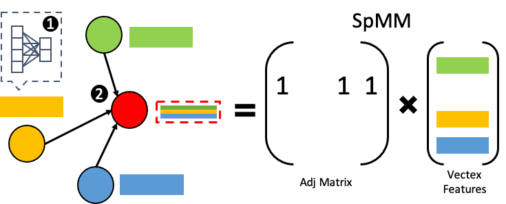
Figure 1: Basic operations of a typical GNN layer (left). Given graph data with vertices, edges, and vertex features, a GNN layer: (1) feeds the features to an MLP (feature extraction) using the GEMM operation; (2) sums the features from the neighborhood (feature aggregation) using an SpMM operation (right).

Independently, edge sampling techniques [13, 14, 15] proposed by researchers allow the training of possibly deeper and more accurate GNN models by solving the over-smoothing and over-fitting problems [16, 17, 18]. Since edge sampling reduces the number of connections in the graph, which in turn reduces SpMM computation time, it could potentially be used to speed up the SpMM kernel. However, existing methods requires preprocessing the graph on the CPU [13] or using a complex model to sample the edges [15]. The resulting added overheads eventually eclipse the benefit of reduced computational complexity.

To more efficiently leverage edge sampling for GNN acceleration, we introduce ES-SpMM, a sampling algorithm and codesigned SpMM kernel to speed GNN inference performance. Key ES-SpMM concepts include: (1) an in-kernel sampling mechanism, which eliminates preprocessing overheads and leverages a GPU’s parallel computing power to accelerate the sampling process, (2) a cache-first edge sampling design that fits the entire sampled graph on a GPU’s shared memory by using the shared memory size as the sampling target, reducing compute load while improving cache locality, (3) coalesced global memory access to efficiently fetch the sampled graph data and load shared memory. (4) and two lightweight sampling strategies to use in conjunction with the kernel to achieve optimal speedup with minimal accuracy. The two strategies offer different trade-offs between model accuracy and speedup and are adaptable to the dataset specifics. Using these novel optimizations and designs, ES-SpMM significantly outperforms state-of-the-art SpMM implementations with negligible accuracy loss for GNNs’ workloads.

To verify the effectiveness of our design, we integrated ES-SpMM into DGL, a popular graph learning library that provides state-of-the-art GNN runtime performance. We designed ES-SpMM to work with the standard CSR (Compressed Sparse Row) format to avoid format transformation overhead, which lets us seamlessly swap DGL’s backend SpMM kernel with ES-SpMM with no modification to user-level code. While the proposed techniques in ES-SpMM are sufficiently general to benefit both GNN training and inference, we focus here on inference only. We conducted comprehensive experiments using two popular GNN models, GCN and GraphSage, on four representative graph benchmarks. Our evaluation results for inference time show that ES-SpMM outperformed cuSPARSE by up to 4.35x with no accuracy loss and 45.3x with less than a 1% accuracy loss.

In sum, our main contributions include:

• The design and implementation of ES-SpMM, a cache-first edge sampling mechanism and SpMM kernel codesign, to speed up GNN inference.

• A novel in-kernel edge sampling mechanism that accelerates the sampling process and eliminates the preprocessing overhead.

• Two lightweight sampling strategies to achieve optimal speedup with minimal accuracy loss across different datasets.

• Standard CSR format support and the integration with a popular GNN framework, DGL, without touching user-level code.

• Comprehensive evaluations on representative GNN models and datasets to verify ES-SpMM’s significantly improved inference efficiency.

• To the best of our knowledge, ES-SpMM is the first work that uses edge sammpling to accelerate GNN inference.

II Background and Motivation

In this section, we now briefly describe the GNN, the Compressed Sparse Row (CSR) format, GPU preliminaries, relevant SpMM optimization on GPUs, and the current state of the GNN computational bottleneck.

II-A Graph Neural Networks

GNNs target feature-rich graphs with have high-dimensional, dense features associated with nodes or edges. A typical GNN has a multi-layer structure. Within a layer, it uses an MLP to extract high-level features from the input features, aggregate the extracted features based on the graph structure and apply an activation function like ReLU on the output features (see Figure 1). Activated features become the input features for the next layer. The final layer’s output features are then be used for downstream prediction tasks, such as node classification or edge prediction.

GNNs differ from basic neural networks mainly due to feature aggregation. Among the different feature aggregation methods, Sum is the most commonly used feature aggregator. In Sum aggregation, a node’s new features are the sum of its neighborhood nodes’ features. Equation 1 shows the formalized computation of a GNN layer using Sum aggregation. $H^{(l)}$ and $W^{(l)}$ are node features and MLP weights for layer $l$, $A$ is the adjacency (adj) matrix, $\sigma(\cdot)$ is the activation function, and the output of the equation becomes the next layer’s node features ($H^{(l+1)}$).

$$H^{(l+1)}=\sigma(AH^{(l)}W^{(l)})$$ (1)

Here, the computation of $H^{(l)}W^{(l)}$ is essentially a GEMM since both $H$ and $W$ are dense matrices. The multiplication of $A$ and $H^{(l)}W^{(l)}$ is an SpMM operation because $A$ is a sparse matrix and the result of $H^{(l)}W^{(l)}$ is a dense matrix. Since Sum is an effective aggregator and adopted by many GNN models [1, 2, 19, 20, 17, 21, 22, 23, 24], in this work we focus on accelerating the GNNs using Sum aggregation.

Figure 2: An example of the CSR sparse format. CSR represents a sparse matrix with three arrays: data, col_ind (column indices), and row_ptr (row pointers). For an unweighted graph’s adjacency matrix, $data$ is an array of 1.

II-B Compressed-Sparse Row (CSR) Format

Sparse formats efficiently store sparse data; in the context of GNN, the sparse adjacency matrix is stored in a sparse format, which skips all zero values to compress the matrix.

There are several common sparse formats. Here, we introduce the most standard one, CSR (see Figure 2). CSR has three arrays to represent a 2D sparse matrix. The first, the data array, keeps all non-zero values following the row-major order. For an unweighted graph’s adjacency matrix, non-zero values are all ones, which is a common case in GNNs’ workloads. The second, col_ind (column indices), keeps column indices of each non-zero value and uses the same order as the data array. The third, row_ptr (row pointers) array, records the accumulated number of non-zero (NNZ) values for each row.

Due to its high efficiency and simplicity, CSR has been adopted by virtually all of the platforms that support sparse operations. Further, most graph matrices come in the CSR format. Therefore, we design ES-SpMM to directly work with this format. By supporting CSR, ES-SpMM can serve as a drop-in replacement for any existing sparse system without the need to transform formats and incurring resulting large overheads.

TABLE I: Statistics of the evaluated graph datasets.

Dataset	# Node	# Edge	Avg. Degree	# Class
Pubmed	19.7K	88.6K	4.5	3
Arxiv	169K	2.3M	13.7	40
Proteins	132K	79.1M	597	112
Reddit	233K	115M	493	41

II-C GPU Preliminaries

We next briefly introduce the GPU hardware architecture and execution model, using NVIDIA’s terminology since this work is implemented in CUDA.

In terms of hardware architecture, a GPU is composed of an array of streaming multiprocessors (SMs). Each SM consists of a few blocks of 32 CUDA cores, where a CUDA core is the smallest compute unit on the GPU. It also has a piece of on-chip, software-managed shared memory (L1 cache) and a pool of registers. Beyond the SM level, there is an L2 cache and a large off-chip global memory shared by all SMs.

For the execution model, a GPU kernel is typically executed by thousands of parallel threads, grouped into thread blocks; each thread block is mapped to an SM. A thread block is further divided into warps, where each warp consists 32 threads. A warp of threads is mapped to a block of 32 CUDA cores and executes the same instruction simultaneously; thus, this execution model is called Single Instruction Multiple Threads (SIMT). The warps in a thread block are streamed into the SM by a hardware scheduler. When a warp is idle, e.g., waiting for memory requests, the warp is context switched out in favor of other warps and is continued later. Therefore, given sufficient warps in a thread block, it’s possible to hide the memory latency with this execution model. Furthermore, a GPU tries to combine memory requests from a warp into as few global memory transactions as possible.

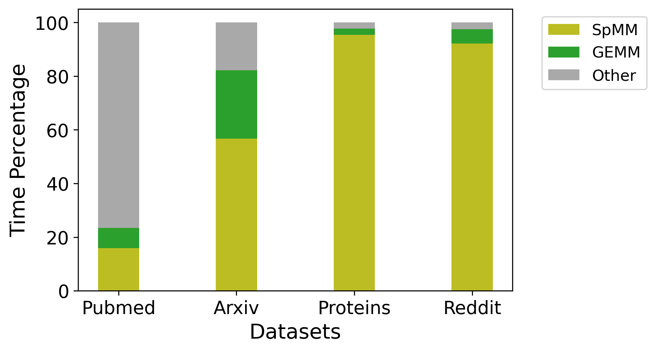
Figure 3: End-to-end compute time breakdown of the GCN model on different datasets.

II-D Performance Bottleneck of GNNs

To illustrate the performance bottleneck of GNNs, Figure 3 breaks down the computation time of GCN [1], a popular GNN model, for four different graph datasets. The GCN model is implemented in DGL, which uses the cuBLAS and cuSPARSE libraries for the GEMM and SpMM operations, respectively. The experiments are conducted on an AWS p3.2xlarge instance with a NVIDIA’s V100 GPU. The statistics of the evaluated datasets and the model setup are shown on Table I and Table III. The detailed descriptions of the datasets and models are in Section V-B.

As Figure 3 shows, despite the use of the highly optimized cuSPARSE library, the performance bottleneck of GNNs still lies in the SpMM kernel. For the smaller datasets, such as Pubmed and Arxiv, the SpMM kernel takes 16% and 56% of the end-to-end compute time, respectively. For the larger datasets, such as Proteins and Reddit, the SpMM kernel consumes an unacceptale 95.4% of the total inference time.

These dramatic results are due to GPUs being optimized for dense and regular operations. SpMM’s sparse and irregular features make it difficult to achieve high throughput on a GPU. As the scale of the graphs involved in GNNs’ workloads becomes progressively larger [25], the compute bottleneck on the SpMM kernel becomes increasingly more severe and hinders the development of larger, deeper GNN models.

To relieve the compute bottleneck and further accelerate GNN inference, we propose a novel SpMM kernel that we codesigned with an edge sampling mechanism to achieve an order of magnitude speedup over existing SpMM kernels.

III Edge Sampling for GNN’s Inference

To demonstrate how we leverage edge sampling to accelerate SpMM kernel performance, in this section we briefly introduce edge sampling techniques in the context of GNNs, analyze its impacts on inference accuracy, and examine the limitations of existing methods.

III-A Edge Sampling

Edge sampling is a technique to include only a subset of edges of the original graph while discarding the rest. The existing methods include randomly dropping edges [13, 14] or using a learned neural network to determine which edges to abandon [15]. Figure 4 highlights the edge sampling process.

To date, edge sampling has been used to mitigate GNN’s over-fitting and over-smoothing [16, 17, 18] training problems. For example, DropEdge [13] randomly samples a different subset of edges throughout training iterations with a fixed dropping rate. The results of DropEdge shows that such dynamic random edge sampling improves training accuracy for both shallow and deep GNN models.

However, rather than improving training accuracy, we for the first time use edge sampling to accelerate GNN’s inference.

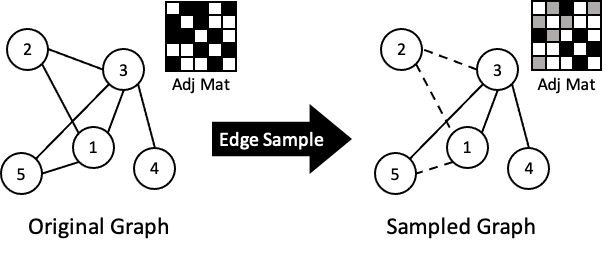
Figure 4: The edge sampling process. The NNZ of the adjacency matrix for the sampled graph is reduced compared to the original graph.

III-B Inference Accuracy

Unlike previous edge sampling works for GNN training have training loops and backpropagation to adapt the loss of edges, model accuracy will likely diminish with the edge-sampled graph during inference, as some graph information is lost in the process of sampling. To understand whether edge sampling is applicable to GNN inference with an acceptable accuracy loss, we conducted an analysis of its effect on inference accuracy.

We mimiced DropEdge [13] by dropping a fixed rate of edges for a given graph, fed the sampled graph to a pre-trained GNN model to obtain test accuracy, and swept the drop rate from 20% to 80%. Figure 5 shows results with the GCN [1] model on four representative datasets.

On Figure 5, we observe that the inference accuracy of the GCN model generally declines as the drop rate increases. For small datasets such as Pubmed and Arxiv, accuracy remains close to the baseline when the edge drop rate falls below 40%. For large datasets such as Proteins and Reddit, accuracy is less sensitive to larger drop rates compared to smaller datasets, and we observe only a small loss even when the edge drop rate reaches 80%.

This analysis shows that a pre-trained GNN model can resist the loss of edges, which provides an opportunity to trade off accuracy and latency. We leverage this fact in our design of ES-SpMM.

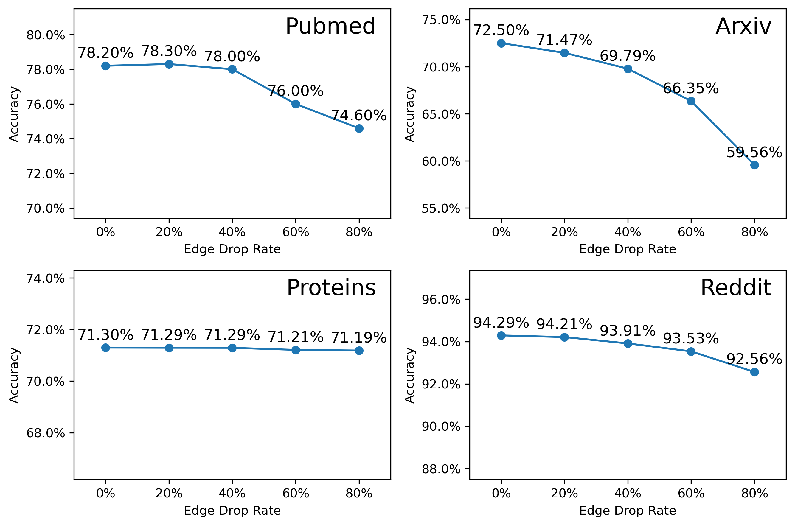
Figure 5: GCN’s [1] inference accuracy when feeding sampled graphs with different edge dropping rates on different datasets. The dropped edges are randomly selected.

III-C SpMM Time Reduction and Sampling Time

As shown in Figure 4, edge sampling reduces the NNZ of the sampled graph’s adjacency matrix, which can diminish the runtime of the SpMM kernel since less computation is needed. However, it requires extra compute time to perform edge sampling. Therefore, an important question becomes whether edge sampling can bring a net end-to-end speedup.

TABLE II: GCN’s [1] SpMM kernel time for running inference with the original and edge-sampled graphs, edge sampling time, and the overall inference slowdown after combining the new SpMM kernel time and sampling overhead, for different datasets. The edge sampling is implemented in NumPy, and the drop rate is 20%. The time is measured in milliseconds.

Dataset	SpMM Time		SpMM	Sample	Overall
	Ori.	Sampled	Speedup	Time	Slowdown
Pubmed	0.68	0.65	1.05x	4.24	2.1x
Arxiv	14	13.1	1.07x	108.5	5.2x
Proteins	173.2	149.4	1.16x	13528	75.7x
Reddit	99.86	89.1	1.12x	6814	63.8x

To answer this question, we conducted another analysis to access how much a SpMM kernel can be accelerated using an edge-sampled graph and how much compute time it takes to perform edge sampling. We follow the same settings as Section II-D and use cuSPARSE’s SpMM kernel to conduct this analysis. We continued to mimic [13] for sampling methodology. We implemented edge sampling in NumPy, the standard way used in [13], and randomly dropped 20% of the edges for each graph. We chose a 20% drop rate here because the tested model maintained near baseline accuracy with this rate, as Figure 5 shows. Table II shows the comparison.

As shown in Table II, the SpMM kernel time is generally faster with the sampled graph, with a speedup range from 1.05x to 1.16x. However, when we consider edge sampling time, the net inference time becomes significantly slower due to the huge number of computing cycles spent on the sampling itself. Using the Reddit dataset as an example, although the SpMM kernel runs 1.12x faster with the sampled graph, edge sampling consumes 6814 ms to run, which results in a 63.8x slower end-to-end inference time. Here, the used random edge sampling strategy is considered lightweight. If we use a more complicated sampling method, such as a neural network model [15], the gap between the sampling time and the SpMM kernel time reduction would be even larger.

As a result, applying existing edge sampling methods on existing SpMM kernels cannot yield a net acceleration to GNN inference, especially with the condition that the graph would be processed only once. We therefore, propose ES-SpMM, a novel cache-first edge sampling mechanism and SpMM kernel codesign that efficiently leverages edge sampling to significantly accelerate GNN inference.

IV CacheSample Kernel Design

We now provide a detailed description of ES-SpMM design, with the goal of leveraging edge sampling to speedup SpMM, the compute bottleneck of GNN inference, while minimizing edge sampling overhead.

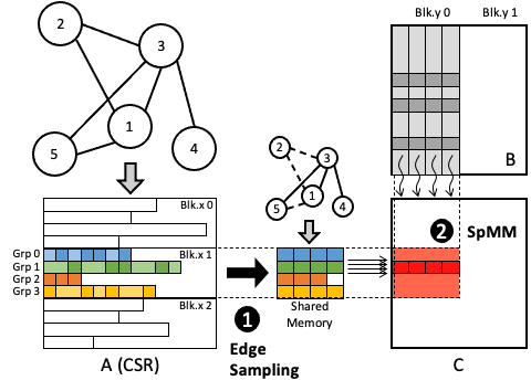
Figure 6: Overview of the ES-SpMM kernel. A, a sparse matrix in CSR format, represents the original graph structure. B contains nodes’ features, and C contains output features. Both of them are dense matrices in the row-major ordering. There are two main stages in ES-SpMM: (1) performing edge sampling and loading the complete edge-sampled graph into shared memory; (2) performing SpMM based on the sampled graph. When loading A’s values, a group of threads share the workload of one row of A, which parallelizes the sampling process. When loading B’s values, threads in the same group load data in the neighboring columns, which creates coalesced memory access. Each thread computes the result of each C’s element.

IV-A Overview

Figure 6 presents an overview of ES-SpMM’s kernel architecture. Input to the kernel is a sparse matrix $A$ in CSR format, which represent the graph structure. A dense matrix $B$ contains the nodes’ features. The output of the kernel is a dense matrix C, which contains the output nodes features. Dense matrices $B$ and $C$ are both in row-major format.

The main computations in ES-SpMM include edge sampling, which shrinks the sparse matrix $A$ to fit on the GPU’s shared memory, and a SpMM operation, compute the output features $C$ based on the sampled graph. Algorithm 1 lists the pseudo code of ES-SpMM. We describe each design step in the following subsections.

1:  Input: A.data, A.row_ptr, A.col_ind, B, shmem_width

2:  Output: C

3:  for each thread do

4:     __shared__ sh_data[], sh_cols[];

5:     row_id, col_id, sh_offset, row_nnz = get_offsets();

6:     S = min(row_nnz, shmem_width);

7:     for $i\leftarrow$ sh_offset to $S$ step $blockDim.x$ do

8:        sample_idx = get_sample_index($i$, row_nnz);

9:        sh_data[i], sh_cols[i] = load_A(sample_idx);

10:     end for

11:     __syncthreads();

12:     acc = 0;

13:     for $j\leftarrow 0$ to $S$ do

14:        acc += sh_data[j] $\ast$ B[sh_cols[j], col_id];

15:     end for

16:     C[row_id, col_id] = acc;

17:  end for

Algorithm 1 Pseudo Code of CacheSample

IV-B Stage 1: Perform Cache-First Edge Sampling

To perform edge sampling in ES-SpMM, we first set a desired shared memory width, $S$. Then, the size of the shared memory each thread block can request is determined by $(\#\>of\>thread\>groups\times S)$. Note that this size is limited by the shared memory capacity of the GPU. The value $S$ also serves as the sampling target for ES-SpMM to downsize the graph data. As shown in Figure 6, for each row of A, at most $S$ non-zero values are fetched to shared memory. If $S$ exceeds the NNZ of that row, then the whole row is fetched to shared memory. In this way, the edge-sampled graph can be fitted to the shared memory within the scope of each thread block. We refer to this sampling mechanism as ”cache-first edge sampling”.

The cache-first edge sampling mechanism offers two main benefits: The first is the reduced computation time required by the SpMM operation in the next stage; the second is improved cache locality from keeping all the needed graph data on shared memory. This is not feasible for existing SpMM kernel implementations because they must ensure the completeness of the SpMM operation, and GPU’s shared memory is usually not large enough to hold all graph data without sampling. However, our proposed cache-first edge sampling scheme exploits the fact that a GNN model can tolerate the loss of edges, and discards redundant edges for better cache locality and faster runtime.

To perform the proposed cache-first edge sampling efficiently, we assign a group of threads to sample a row of $A$ in ES-SpMM. Here, each thread uses one of the lightweight sampling strategies (Section IV-D) to compute the sampling indices and loads the selected A’s data and column indices into shared memory. We arrange 32 to 128 threads in each thread group. Depending on the size of each thread group, we arrange 4 to 8 thread groups in a thread block, forming a fixed 512 threads in each thread block. As the thread groups in the same thread block share the same shared memory space, each shared memory block holds 4 to 8 rows of $A$’s sampled values. In the SpMM operation, the next stage of ES-SpMM, all values of A come from shared memory, and the kernel computes the SpMM only for the sampled values.

As noted in Section III-C, edge sampling can cause substantial compute overhead that retards overall runtime. ES-SpMM therefore, parallelizes the sampling task into thousands of threads and significantly accelerates it. Such in-kernel sampling also eliminates the need to preprocess graph data on the CPU and lets user-level code remain untouched when using the ES-SpMM as the back-end SpMM kernel. In this way, although edge sampling must be re-computed each time the kernel is launched, our evaluation results (Section V) show that ES-SpMM can still yield massive acceleration, which indicates that our parallelized edge sampling design is very efficient.

IV-C Stage 2: Compute SpMM Based on Sampled Results

Once edge sampling is done and shared memory is loaded, the second stage of ES-SpMM begins, which aims to compute the SpMM based on sampled results. Since ES-SpMM computes the multiplications only for the sampled A’s values, it approximates the SpMM.

Operations in this stage are straightforward, including reading A’s data and column indices from shared memory, loading the corresponding B’s data from global memory, calculating the product, and looping to repeat these process and accumulate multiplication results. Algorithm 1, lines 12 to 16, shows the pseudo code for this stage.

To perform these operations, ES-SpMM assigns to each thread the computation task for an element of C. This thread management resembles SpMM kernel optimizations in [8] and [7]. However, the major difference is that all needed A’s values in ES-SpMM are loaded to shared memory prior to this stage. Therefore, the clean and dedicated loop here needs no synchronization or extra data loading, which means that ES-SpMM has fewer branch divergences and can achieve a higher ILP.

After the sampled SpMM is computed, each thread stores the multiplication result of an element of C from a local register to global memory, and ES-SpMM kernel operations are finished. The whole ES-SpMM process is implemented in roughly 50 lines of CUDA code.

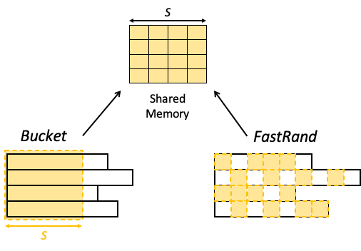
Figure 7: Overview of ES-SpMM’s two edge sampling strategies, Bucket and FastRand. Bucket takes the first $S$ continuous A’s values. FastRand samples across the whole region in a pseudo-random manner.

IV-D Sampling Strategy

Section IV-B stated that within the cache-first edge sampling mechanism, ES-SpMM could use different lightweight sampling strategies for each thread to compute exact sampling indices (see line 8 in Algorithm 1). We now specify the design of the strategies.

A primary design consideration for ES-SpMM’s sampling is efficiency. Although we use parallel threads to accelerate edge sampling (Section IV-B), computation of the sampling itself must still be lightweight to maximize ES-SpMM performance. Based on this consideration, we designed two lightweight edge sampling strategies, Bucket and FastRand, with different speedup and accuracy impacts. Figure 7 highlights each strategy, which we describe below.

Bucket. Given the target shared memory width, $S$, the Bucket edge sampling strategy picks the first $S$ non-zero data and column indices for each row of $A$. We call this strategy Bucket because it resembles the way a bucket carries items to fit a specific volume. Bucket is very fast since it needs only a boundary check to determine which indices to keep. However, we found that it could significantly sacrifice accuracy, especially on large graphs because it maintains a fixed range of edges for each node. See Section V for more information on Bucket’s accuracy.

FastRand. As noted in Section III-B, GNN’s inference accuracy can be well preserved using a random edge sampling scheme, especially for large graphs with numerous nodes and edges. Based on this observation, we designed the FastRand edge sampling strategy to perfor a pseudo-random sampling for ES-SpMM. To attain both good randomness and fast speed, FastRand uses an efficient hash function to calculate sample indices; Equation 2 shows the hash function.

As Equation 2 shows, to calculate the sample index ($sample\_idx$) for a given shared memory location ($shmem\_idx$), FastRand multiplies $shmem\_idx$ with a prime number $P^{\prime}$ and takes a modulo over the $row\_nnz$, which is the NNZ of the targeted row. Then, ES-SpMM uses $sample\_idx$ as the index value to fetch A’s data and column indices and store them to the shared memory at position $shmem\_idx$ (see line 9 in Algorithm 1). Note that in order to sample across the full range of non-zero values for each row of A, the prime number $P^{\prime}$ cannot be too small. In practice, we chose $P^{\prime}=577$ when implementing the ES-SpMM kernel. In this way, FastRand fulfills the pseudo-random edge sampling using only one multiplication and one modulo operation, which are sufficiently lightweight for each GPU thread to finish within a short latency. With this type of sampling, we expect the accuracy loss of FastRand to be less than Bucket. However, we expect Bucket to be faster since it needs less computation. See Section V for our detailed evaluation.

$$sample\_idx=(shmem\_idx\times P^{\prime})\mod row\_nnz$$ (2)

IV-E Kernel Optimizations

In addition to cache-first edge sampling and the sampled SpMM, ES-SpMM uses other kernel optimizations to achieve optimal performance. We now describe these.

IV-E1 Thread management

Per Section IV-B, we use up to 128 threads to handle the sampling and data loading for each row of $A$ in ES-SpMM. This is unique since a common thread management approach adopted by many existing SpMM kernel optimizations [8, 7, 12, 11] uses a warp (32) of threads to load a row of A’s values to registers or shared memory. Previous works use this thread setting to provide an acceptable balance of parallelism and number of tasks per thread for SpMM workloads. However, unlike the previous SpMM kernels, which usually load only a partial row at one time, ES-SpMM must complete the sampling and data loading for an entire row in one stage. Because the targeted shared memory width, $S$, could be large (such as 512), using only 32 threads for a row requires multiple iterations to completely load the shared memory, which may slow down both sampling and data loading. Therefore, we use up to 128 threads to sample and load a row of $A$ in ES-SpMM to improve performance.

IV-E2 Coalesced memory access

Coalesced memory access is an important optimization to reduce memory loading latency on GPU. In the second stage of ES-SpMM, we allowed a group of threads to load B’s data in the same row but in neighboring columns at the same time. This coalesces memory access because the data requests from multiple threads can be combined and fulfilled by fewer global memory transactions. As a result, data loading for B in ES-SpMM is very efficient. This technique resembles those introduced in [8, 7].

IV-E3 Load balancing

It is natural for some nodes to have many more connections than other nodes in the graph, leading to a large variations of the NNZ from row to row, as Figure 6 shows. The irregular distribution can easily result in an unbalanced load for the SpMM kernel and degrade kernel performance, especially under a row-split work distribution. In ES-SpMM, the NNZ variation of each row is limited to the targeted shared memory width, $S$, after edge sampling. In this way, the work assigned to each thread is much better balanced than running on an unsampled graph, helping ES-SpMM achieve higher utilization and improved performance.

V Evaluation

We next describe system integration, experiment setup, and the comprehensive experiments we conducted to verify the effectiveness of ES-SpMM.

V-A Integration with DGL

To maximize the applicability of ES-SpMM to GNN models, we integrated ES-SpMM into one of the most popular GNN frameworks, DGL [26], which provides a set of high-level Python APIs. The backend of DGL calls to the cuSPARSE’s cusparseSpMM() kernel to perform the SpMM operation.

Since both cusparseSpMM() and ES-SpMM work on the standard CSR format, we simply replaced the cusparseSpMM() with our ES-SpMM kernel in the DGL backend for the integration. Because ES-SpMM needs no preprocessing on the graph data, the DGL user-level code remains unmodified during this process.

TABLE III: Model parameters and baseline accuracy we achieve on each dataset for GCN and GraphSage.

Model	Dataset	#Layer	#Hidden	Test Acc
GCN	Pubmed	2	32	77.70%
	arxiv	3	256	72.50%
	proteins	3	256	71.30%
	Reddit	2	128	94.29%
GraphSage	Pubmed	2	32	78.60%
	arxiv	3	256	72.95%
	proteins	3	256	77.28%
	Reddit	2	128	96.22%

V-B Experiment Setup

We now describe the setup we used to conduct our experiments.

V-B1 Evaluated GNN models and datasets

We chose two classic GNN models, GCN [1] and GraphSage [2], and four node classification datasets to evaluate our ES-SpMM kernel. The four graph datasets were Pubmed, Arxiv, Proteins and Reddit. Pubmed is a citation network of medical academic papers. Arxiv and Proteins were taken from the Open Graph Benchmark - Node Property Prediction collection [25]. Reddit is a social network dataset collected from a popular online forum. These four datasets are of different scales in terms of the number of nodes and edge. For GraphSage, we used mean feature aggregation. Hence, experiment results using them can help us appreciate ES-SpMM’s performance for different graph scales. Table III lists the model parameters for each datasets, and Table I shows the dataset statistics.

V-B2 Model setup

We first trained the GNN models on each dataset for ten times with the original DGL framework, and kept the ones with the highest test accuracy. Table III shows the best test accuracy we achieved for each model and dataset. After the models were trained, we used our modified DGL to call ES-SpMM and run the experiments on inference.

V-B3 SpMM baselines

Our experiments compare the performance of ES-SpMM to the following CSR SpMM baselines.

• cuSPARSE: The default implementation in DGL. The main kernel is cusparseSpMM(), and the compute algorithm is set to CUSPARSE_SPMM_CSR_ALG2 [27], as it achieves the best performance in our setup.

• Merge-SpMM: Proposed in [8]. It has a suite of different row-split and merge-based algorithms aimed at improving load balance. The code is available at [28]. To test this kernel, we ran it with all proposed algorithms and picked the highest performer in each case.

• GE-SpMM: Proposed in [7]. It is based on the row-split design of [8] but has an improved shared memory usage. We also ran all kernel setup provided in their open-source package [29] and picked the best performer.

V-B4 Hardware environment

Our experiments were conducted on the following hardware environment.

• AWS EC2 p3.2xlarge instance. GPU model: NVIDIA V100 with 16GB global memory. CUDA version: 11.0. CPU: Intel Xeon E5-2686 v4 (8 virtual cores) with 61GB main memory.

V-C Sampling Rate

As noted in Section III-B, sampling rate is an important factor affecting inference accuracy. In ES-SpMM, the target shared memory width, $S$, determines the sampling rate. Since each graph has a different distribution of nodes and edges, its sampling rate under each $S$ value is different in ES-SpMM.

To obtain the sampling rates, we simulated the cache-first edge sampling mechanism in Python and calculated the equivalent sampling rates for each $S$. Table IV shows the sampling rates for each dataset. Note that Bucket and FastRand have the same sampling rate for a given $S$ since they fetch the same amount of A’s values to shared memory.

Per Table IV, for small graphs such as Pubmed and Arxiv, a small $S$ (16) already holds over 80% percent of the edges, and a larger $S$ (above 128) actually holds over 99% of the edges. However, for large graphs such as Proteins and Reddit, the sampling rates are much lower compared to the small graphs under a fixed $S$. For example, when $S=256$, the sampling rates are only around 34% for Proteins and Reddit but are 100% and 99.9% for Pubmed and Arxiv. Based on our sampling rate analysis, we expect that ES-SpMM will experience little to no accuracy loss for small graphs but a more sizable accuracy loss for large graphs, especially when $S$ is small.

TABLE IV: Sampling rates under different $S$ values for different datasets in ES-SpMM.

Dataset	s=16	s=32	s=64	s=128	s=256	s=512
Pubmed	84.9%	95.8%	99.3%	99.9%	100.0%	100.0%
Arxiv	83.7%	96.8%	99.3%	99.8%	99.9%	100.0%
Proteins	2.6%	5.1%	9.9%	18.9%	34.3%	56.7%
Reddit	3.1%	6.0%	11.3%	20.5%	34.8%	53.9%

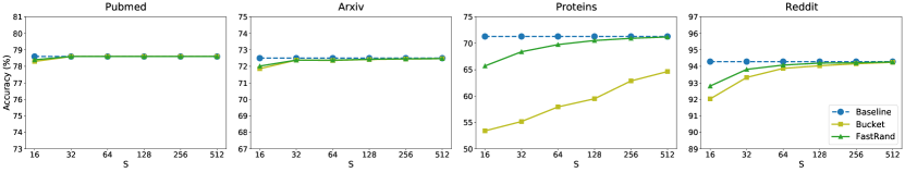
(a) GCN inference accuracy.

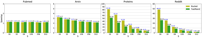
(b) SpMM kernel speedup for GCN.

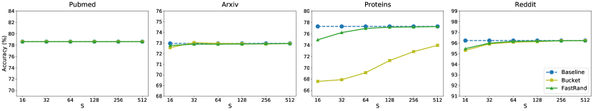
(c) GraphSage inference accuracy.

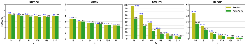
(d) SpMM kernel speedup for GraphSage.

Figure 8: ES-SpMM’s accuracy and SpMM speedup compared to cuSPARSE under different $S$ values (ES-SpMM’s target shared memory width) for GCN and GraphSage. The experiments were run on NVIDIA V100 GPU.

V-D Benefits of ES-SpMM

We now present the inference accuracy and speedup of using ES-SpMM compared to cuSPARSE SpMM kernel.

V-D1 Inference accuracy and speedup under different $S$ values

To conduct these experiments, we first ran GCN and GraphSage with the unmodified DGL, which uses cuSPARSE’s SpMM kernel, to assess baseline inference accuracy and SpMM kernel time for each dataset. Here, we used PyTorch Profiler [30] to measure SpMM kernel time. Then, we ran the inference with our modified DGL that uses the ES-SpMM kernel, swept $S$ from 16 to 512, and compared the test accuracy and SpMM performance. For SpMM performance, we compared the total SpMM kernel time of a complete inference and we took the average after running the inference 10 times. Figure 8 shows experimental results on the accuracy and SpMM speedup against cuSPARSE.

For accuracy on the small datasets, Pubmed and Arxiv, ES-SpMM generally had little to no accuracy loss across different $S$ values for both Bucket and FastRand. For GraphSage on Pubmed, ES-SpMM had no accuracy loss even when $S$ was as small as $16$. This echoes the discussion in Section V-C since ES-SpMM can hold most edges with a small $S$ for small graphs.

For SpMM speedup on small datasets, ES-SpMM achieved 1.1x to 4.35x speedup compared to cuSPARSE. For Pubmed, ES-SpMM achieved roughly 1.1x and 4x speedup for GCN and GraphSage respectively, across all $S$ values. We saw a smaller speedup for GCN because the baseline SpMM kernel time was already short (0.64ms). The steady speedup across different $S$ values occurred because the sampling rates were at a similar level (Table IV). On Arxiv, ES-SpMM’s speedup slightly decreased when $S$ went up. This is due to increased sampling overhead with a larger $S$, which diminished ES-SpMM’s performance. However, even with a large $S=512$, ES-SpMM still achieved at least a 2.15x and 2.35x speedup for GCN and GraphSage respectively, on Arxiv.

Regarding accuracy on the datasets Proteins and Reddit, ES-SpMM experienced a larger loss of accuracy but still achieved near-baseline accuracy with a larger $S$ value. Also, on these larger graphs, FastRand generally exhibited better accuracy than Bucket. For example, on Proteins, Bucket had a large accuracy loss even when $S=512$. In our experiments, we found that $S$ must be as large as $1792$ to achieve less than a 1% accuracy loss when using Bucket on Proteins. However, for FastRand, it achieved near-baseline accuracy with $S=128$ for GCN and $S=64$ for GraphSage. FastRand also had much lower drop in accuracy than Bucket when $S$ was smaller; this is because the graph degree of Proteins is large, and the Bucket’s method for picking the first continuous edges makes it lose many graph features. On the other hand, FastRand randomly sampled all edges, which preserved graph structure and yield much improved accuracy. For Reddit, we observed an accuracy trend similar to Proteins. However, since Reddit is an easier dataset that both GCN and GraphSage achieve high baseline accuracy (94.3% and 96.2%), Bucket’s accuracy loss on Reddit is not as pronounced as Proteins.

Regarding SpMM speedup on large datasets, ES-SpMM achieved a tremendous speedup agains cuSPARSE for both Bucket and FastRand, due to the low effective sample rates. On Proteins, although ES-SpMM with Bucket achieved up to 81.6x and 96.15x speedup for GCN and GraphSage respectively, it was less meaningful since the accuracy loss was large. However, with FastRand, ES-SpMM achieved a 13x speedup with only a negligible accuracy loss when $S=128$ for both GCN and GraphSage on Proteins. On Reddit, both Bucket and FastRand achieved a meaningful speedup with only a small accuracy loss. When $S=64$, Bucket achieved 12.5x and 11.3x and FastRand achieved 8.72x and 8.75x for GCN and GraphSage respectively, where both strategies showed negligible accuracy loss, a significant benefit due to ES-SpMM.

TABLE V: ES-SpMM’s best SpMM speedup against cuSPARSE with less than 1% accuracy loss.

Model	Dataset	$S$		Accuracy			Accuracy Loss		SpMM Time (ms)			SpMM Speedup
		Bucket	FastRand	Baseline	Bucket	FastRand	Bucket	FastRand	Baseline	Bucket	FastRand	Bucket	FastRand
GCN	Pubmed	16	16	77.70%	77.30%	77.50%	0.40%	0.20%	0.64	0.56	0.56	1.13	1.13
	Arxiv	16	16	72.50%	71.86%	72.02%	0.64%	0.48%	12.39	3.81	3.91	3.25	3.17
	Proteins	1792	128	71.30%	70.72%	70.53%	0.58%	0.77%	172.92	71.93	13.07	2.40	13.23
	Reddit	32	32	94.29%	93.33%	93.82%	0.96%	0.47%	99.74	3.90	6.62	25.59	15.06
GraphSage	Pubmed	16	16	78.60%	78.60%	78.60%	0.00%	0.00%	3.56	0.82	0.87	4.35	4.10
	Arxiv	16	16	72.95%	72.55%	72.75%	0.40%	0.20%	18.83	5.32	5.33	3.54	3.53
	Proteins	2304	64	77.28%	76.47%	76.92%	0.81%	0.36%	237.50	140.02	10.25	1.70	23.16
	Reddit	16	16	96.22%	95.30%	95.46%	0.92%	0.76%	449.69	9.93	16.74	45.30	26.87

V-D2 Speedup with less than 1% accuracy loss

Here, we set a 1% accuracy loss constraint and report the best ES-SpMM SpMM speedup, the corresponding $S$ value, and inference accuracy for each sampling strategy in Table V; we still compare to cuSPARSE for speedup. We set this constraint because we assume that a 1% accuracy loss is an acceptable cost to trade off for a faster GNN inference time. In other words, if users can accept a minimally higher accuracy loss, then ES-SpMM can deliver a more significant speedup.

As Table V shows, for most of cases, $S=16$ was sufficient for ES-SpMM to meet this constraint. For the small datasets, ES-SpMM achieved up to 3.25x for GCN and 4.35x for GraphSage, both using Bucket. For the large datasets, ES-SpMM generally offered an over 10x speedup against the strong cuSPARSE baseline, which is significant. The best SpMM speedup ES-SpMM achieved for Proteins and Reddit under this constraint were 23.16x with FastRand and 45.3x with Bucket. The only exception was that ES-SpMM needed a large $S$ to meet this constraint when using Bucket on Proteins. However, ES-SpMM with Bucket still achieved a profitable 2.4x and 1.7x speedup for GCN and GraphSage respectively, with $S=1792$ and $S=2304$.

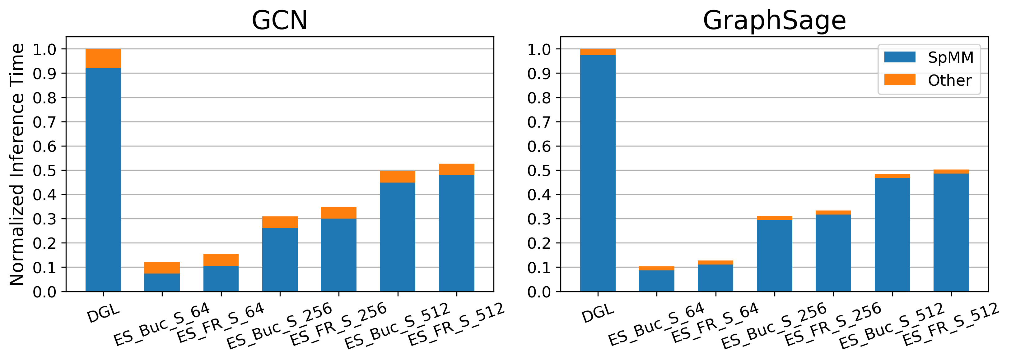
Figure 9: End-to-end inference time breakdown of GCN and GraphSage on Reddit, using the original DGL (calls to cuSPARSE) and ES-SpMM with different $S$ values. The time is normalized to DGL’s result for each model respectively.

V-D3 End-to-end inference time

Here we compare the end-to-end inference time of using ES-SpMM to the original DGL’s results, which uses cuSPARSE for its SpMM operation. Figure 9 shows the end-to-end inference time breakdown of running GCN and GraphSage on Reddit with the original DGL and with the ES-SpMM in different $S$ values. As noted in Section II-D: SpMM consumes a large portion of GNN inference time, and noted in Section V-D1: ES-SpMM significantly accelerates the SpMM operation, the end-to-end inference time was considerably reduced when using ES-SpMM as Figure 9 shows. ES-SpMM achieves about 10x faster end-to-end inference time for both models compared to the original DGL, when using a small $S$ (64). When using a large $S$ (512), ES-SpMM still achieves roughly 2x speedup.

V-E SpMM Performance Compared to Open-Source Baselines

Besides cuSPARSE, we compared ES-SpMM’s SpMM performance to Merge-SpMM’s and GE-SpMM’s.

To conduct these evaluations, we did not modify the open-source packages of Merge-SpMM and GE-SpMM, and fed the SpMM kernels with the adjacency matrix extracted from DGL. This methodology prevented us from changing kernel behavior while re-implementing the kernels into DGL’s backend. To get a similar comparison to the one we achieved in Section V-D, we separately performed multiple SpMM operations that were needed for a complete inference, and combined the kernel times to get total SpMM time. We also did the same operations on cuSPARSE and ES-SpMM for a fair evaluation. The results we show are the average of 200 runs.

Figure 10 shows the SpMM time comparison of running GCN inference on each dataset. For ES-SpMM, we show the results of using $S=32$ and $S=128$ since these settings were generally optimal for ES-SpMM to achieve near-baseline accuracy for small and large graphs. As Figure 10 shows, Merge-SpMM and GE-SpMM only achieved a slightly faster kernel time than cuSPARSE on large graphs. However, ES-SpMM achieved the fastest SpMM kernel time across all datasets and excelled on the large graphs, consuming only 5% to 20% of cuSPARSE’s kernel time.

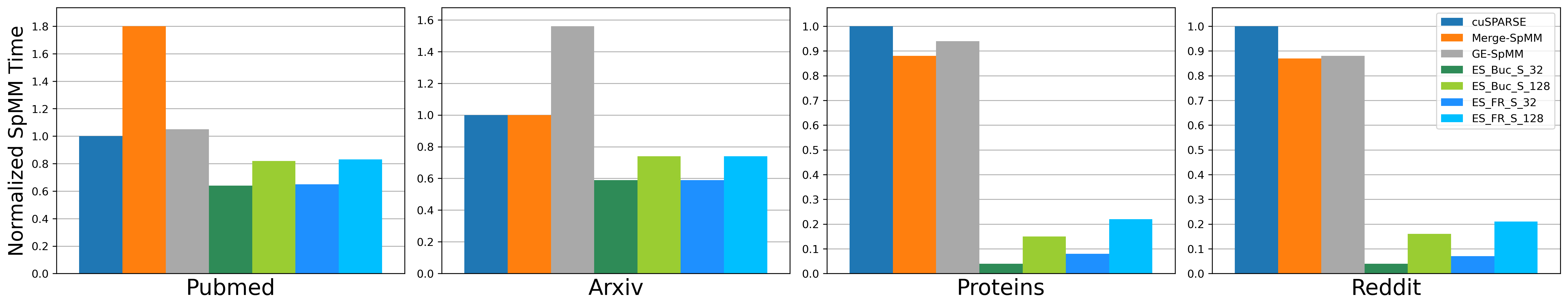
Figure 10: SpMM time of GCN’s inference using different SpMM kernels. The time is normalized to cuSPARSE’s result for each dataset respectively.

V-F Feeding Pre-Sampled Graphs to Baseline SpMM Kernels

To evaluate the source of ES-SpMM’s benefits, we reran an experiment (Section III-C) that fed pre-sampled graphs to the SpMM kernels. Unlike Section III-C experiment doing a general random sampling, here we simulated the FastRand of ES-SpMM in Python for pre-sampling. Then, we fed the pre-sampled graph to cuSPARSE, Merge-SpMM and GE-SpMM and measured the SpMM kernel time. For ES-SpMM, we used the normal graph but set $S$ to the corresponding value. Again, we summed SpMM kernel times for a complete inference and took the average of 200 runs for comparison.

Figure 11 shows the SpMM time comparison of running GCN on original and pre-sampled Reddit with $S=128$ and $256$. As the figure shows, with pre-sampled graphs, all baseline kernels had a dramatically faster kernel time. For Merge-SpMM and GE-SpMM, they actually achieved a similar to slightly better performance than ES-SpMM with pre-sampled graphs. cuSPARSE achieved a slightly slower SpMM time than ES-SpMM, but the results were close. These findings show that the major benefits of ES-SpMM come from the computation reduction enabled by edge sampling. However, additional optimizations (Section IV) helped ES-SpMM achieve a competitive performance with other highly optimized SpMM kernels when the input graph was already edge-sampled. Note that ES-SpMM needed to perform edge sampling in the kernel, which took extra overhead that other SpMM kernels did not have. ES-SpMM’s kernel time can be shortened if we remove time spent on sampling. We didn’t show the results here because such in-kernel time breakdown is difficult to measure.

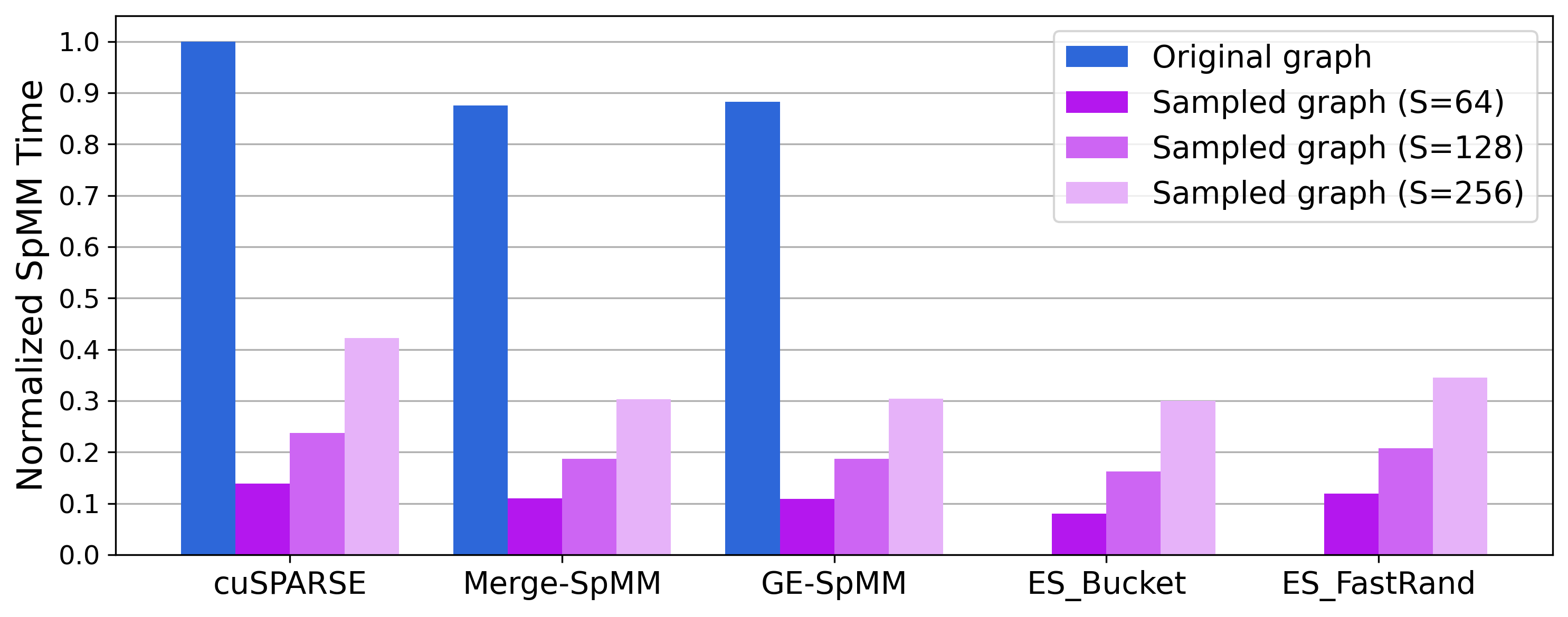
Figure 11: SpMM time of GCN’s inference on Reddit with the original and pre-sampled graphs. The time is normalized to the result of cuSPARSE with the original graph.

VI Discussion and Future Work

VI-A Normalization of GNN

A GNN using sum aggregation, generally it normalizes node features by dividing them with the degree of each node. Practically, a GNN framework like DGL uses a separate operator to handle such normalization. However, this does not work for ES-SpMM since it reduces the number of edges internally in the SpMM kernel without modifying the graph managed by the framework. To make the normalization work, we must remove normalization from the DGL and compute it in the ES-SpMM kernel. Although gaining overhead to compute the normalization, ES-SpMM still achieves a massive speedup and considerable end-to-end acceleration for GNN inference, as Section V shows.

VI-B Accelerate GNN training

Although we focus on accelerating GNN inference in this work, ES-SpMM can be used to accelerate GNN training, which also involves many SpMM operations. However, with our current designs, ES-SpMM would experience lower accuracy when applied to GNN training. Unlike the inference scheme, users are willing to pay more compute time to improve accuracy during training. Therefore, applying ES-SpMM to accelerate GNN training does not make sense.

ES-SpMM reduces training accuracy because it samples the same subset of edges each time for a given graph, sampling strategy (Bucket or FastRand) and $S$ value. As DropEdge [13] suggests, training accuracy can be maintained or improved by taking a different subset of edges throughout training iterations. We expect ES-SpMM could accelerate GNN training without losing accuracy if we would efficiently implement a dynamic random sampling into the ES-SpMM kernel. We leave this to future work.

VI-C Edge Sampling vs. Node Sampling

Besides the edge sampling used in this work, there is another kind of sampling, node sampling, that is used in GNNs. Here we briefly introduce the node sampling, clarify the differences between edge sampling, and discuss ES-SpMM’s applicability to it.

Node sampling is first proposed by [2]. Unlike edge sampling which only takes subsets of edges, node sampling not only takes subsets of nodes but also discards unrelated edges for each subset. The main usage of existing node sampling methods [2, 19, 20, 22, 21] is to extract subgraphs and form the mini-batch training scheme for GNNs, allowing training of very large graphs that cannot be fitted into a single GPU’s global memory.

Although the compute time of each node-sampled graph is much shorter because fewer nodes and edges are presented, it requires multiple iterations to run through the original graph. Therefore, the overall runtime to train or infer for a full graph is increased with node sampling since iterations over different subgraphs incur extra overhead [2, 19]; sometimes, node sampling could even cause high traffics between CPU’s and GPU’s memory [31, 32], which would significantly slowdown both training and inference. We expect ES-SpMM to further improve the inference speed for node-sampled graphs by applying edge sampling. However, the bottleneck will likely be the looping overhead or memory bandwidth contention and thus we expect limited speedup.

VII Conclusion

This work proposed ES-SpMM, a cache-first edge sampling mechanism and SpMM kernel codesign. The ES-SpMM design leverages the fact that a GNN model can tolerate the loss of edges without losing much accuracy for inference. By strategically and efficiently sampling the edges and fitting all sampled edges on GPU’s shared memory, ES-SpMM can significantly accelerate the SpMM operation with minimum accuracy loss compared to other state-of-the-art SpMM kernels. Our experimental results on representative GNN models and datasets show that ES-SpMM outperforms cuSPARSE by up to 4.35x with no accuracy loss and by 45.3x with less than a 1% accuracy loss. To the best of our knowledge, ours is the first work to utilize edge sampling to accelerate GNN inference.

References

- [1] T. N. Kipf and M. Welling, “Semi-supervised classification with graph convolutional networks,” in International Conference on Learning Representations (ICLR), 2017.
- [2] W. L. Hamilton, R. Ying, and J. Leskovec, “Inductive representation learning on large graphs,” in NIPS, 2017.
- [3] M. Allamanis, M. Brockschmidt, and M. Khademi, “Learning to represent programs with graphs,” in International Conference on Learning Representations, 2018.
- [4] P. Battaglia, J. B. C. Hamrick, V. Bapst, A. Sanchez, V. Zambaldi, M. Malinowski, A. Tacchetti, D. Raposo, A. Santoro, R. Faulkner, C. Gulcehre, F. Song, A. Ballard, J. Gilmer, G. E. Dahl, A. Vaswani, K. Allen, C. Nash, V. J. Langston, C. Dyer, N. Heess, D. Wierstra, P. Kohli, M. Botvinick, O. Vinyals, Y. Li, and R. Pascanu, “Relational inductive biases, deep learning, and graph networks,” arXiv, 2018. [Online]. Available: https://arxiv.org/pdf/1806.01261.pdf
- [5] M. Zitnik, M. Agrawal, and J. Leskovec, “Modeling polypharmacy side effects with graph convolutional networks,” Bioinformatics, vol. 34, no. 13, p. 457–466, 2018.
- [6] Y. Hu, Z. Ye, M. Wang, J. Yu, D. Zheng, M. Li, Z. Zhang, Z. Zhang, and Y. Wang, “Featgraph: A flexible and efficient backend for graph neural network systems,” in International Conference for High Performance Computing, Networking, Storage, and Analysis (SC), 2020.
- [7] G. Huang, G. Dai, Y. Wang, and H. Yang, “Ge-spmm: General-purpose sparse matrix-matrix multiplication on gpus for graph neural networks,” 2020.
- [8] C. Yang, A. Buluc, and J. D. Owens, “Design principles for sparse matrix multiplication on the gpu,” in European Conference on Parallel Processing, 2018.
- [9] G. Ortega, F. Vázquez, I. García, and E. M. Garzón, “Fastspmm: An efficient library for sparse matrix matrix product on gpus,” The Computer Journal, 2014.
- [10] S. Gray, A. Radford, and D. P. Kingma, “Gpu kernels for block-sparse weights,” arXiv preprint arXiv:1711.09224, 2017.
- [11] C. Hong, A. Sukumaran-Rajam, I. Nisa, K. Singh, and P. Sadayappan, “Adaptive sparse tiling for sparse matrix multiplication,” in Proceedings of the 24th Symposium on Principles and Practice of Parallel Programming, ser. PPoPP ’19, 2019, p. 300–314.
- [12] T. Gale, M. Zaharia, C. Young, and E. Elsen, “Sparse gpu kernels for deep learning,” 2020.
- [13] Y. Rong, W. Huang, T. Xu, and J. Huang, “Dropedge: Towards deep graph convolutional networks on node classification,” in International Conference on Learning Representations, 2020. [Online]. Available: https://openreview.net/forum?id=Hkx1qkrKPr
- [14] A. Hasanzadeh, E. Hajiramezanali, S. Boluki, M. Zhou, N. Duffield, K. Narayanan, and X. Qian, “Bayesian graph neural networks with adaptive connection sampling,” in Proceedings of the 37th International Conference on Machine Learning, ser. Proceedings of Machine Learning Research, vol. 119. PMLR, 2020, pp. 4094–4104.
- [15] C. Zheng, B. Zong, W. Cheng, D. Song, J. Ni, W. Yu, H. Chen, and W. Wang, “Robust graph representation learning via neural sparsification,” in Proceedings of the 37th International Conference on Machine Learning, ser. Proceedings of Machine Learning Research, 2020.
- [16] Q. Li, Z. Han, and X.-M. Wu, “Deeper insights into graph convolutional networks for semi-supervised learning,” in Thirty-Second AAAI Conference on Artificial Intelligence, 2018.
- [17] K. Xu, C. Li, Y. Tian, T. Sonobe, K. ichi Kawarabayashi, and S. Jegelka, “Representation learning on graphs with jumping knowledge networks,” 2018.
- [18] J. Klicpera, A. Bojchevski, and S. Gunneman, “Predict then propagate: Graph neural networks meet personalized pagerank,” in Proceedings of the 7th International Conference on Learning Representations, 2019.
- [19] J. Chen, T. Ma, and C. Xiao, “FastGCN: Fast learning with graph convolutional networks via importance sampling,” in International Conference on Learning Representations, 2018. [Online]. Available: https://openreview.net/forum?id=rytstxWAW
- [20] W.-L. Chiang, X. Liu, S. Si, Y. Li, S. Bengio, and C.-J. Hsieh, “Cluster-gcn: An efficient algorithm for training deep and large graph convolutional networks,” in Proceedings of the 25th ACM SIGKDD International Conference on Knowledge Discovery; Data Mining, ser. KDD ’19, 2019. [Online]. Available: https://doi.org/10.1145/3292500.3330925
- [21] W. Huang, T. Zhang, Y. Rong, and J. Huang, “Adaptive sampling towards fast graph representation learning,” in Advances in Neural Information Processing Systems (NIPS), 2018.
- [22] H. Zeng, H. Zhou, A. Srivastava, R. Kannan, and V. Prasanna, “GraphSAINT: Graph sampling based inductive learning method,” in International Conference on Learning Representations, 2020. [Online]. Available: https://openreview.net/forum?id=BJe8pkHFwS
- [23] G. Li, M. Müller, A. Thabet, and B. Ghanem, “Deepgcns: Can gcns go as deep as cnns?” in The IEEE International Conference on Computer Vision (ICCV), 2019.
- [24] Z. W. Ming Chen, B. D. Zengfeng Huang, and Y. Li, “Simple and deep graph convolutional networks,” 2020.
- [25] W. Hu, M. Fey, M. Zitnik, Y. Dong, H. Ren, B. Liu, M. Catasta, and J. Leskovec, “Open graph benchmark: Datasets for machine learning on graphs,” arXiv preprint arXiv:2005.00687, 2020.
- [26] M. Wang, L. Yu, D. Zheng, Q. Gan, Y. Gai, Z. Ye, M. Li, J. Zhou, Q. Huang, C. Ma, Z. Huang, Q. Guo, H. Zhang, H. Lin, J. Zhao, J. Li, A. J. Smola, and Z. Zhang, “Deep graph library: Towards efficient and scalable deep learning on graphs,” 2019. [Online]. Available: http://arxiv.org/abs/1909.01315
- [27] NVIDIA, “The api reference guide for cusparse, the cuda sparse matrix library,” 2021. [Online]. Available: https://docs.nvidia.com/cuda/cusparse/index.html
- [28] C. Yang and miheer vaidya, “Merge-spmm open source code,” 2020. [Online]. Available: https://github.com/owensgroup/merge-spmm
- [29] G. Huang, “Ge-spmm open source code,” 2020. [Online]. Available: https://github.com/hgyhungry/ge-spmm
- [30] A. Paszke, S. Gross, F. Massa, A. Lerer, J. Bradbury, G. Chanan, T. Killeen, Z. Lin, N. Gimelshein, L. Antiga, A. Desmaison, A. Kopf, E. Yang, Z. DeVito, M. Raison, A. Tejani, S. Chilamkurthy, B. Steiner, L. Fang, J. Bai, and S. Chintala, “Pytorch: An imperative style, high-performance deep learning library,” in Advances in Neural Information Processing Systems 32.
- [31] Z. Lin, C. Li, Y. Miao, Y. Liu, and Y. Xu, “Pagraph: Scaling gnn training on large graphs via computation-aware caching,” in Proceedings of the 11th ACM Symposium on Cloud Computing, ser. SoCC ’20. New York, NY, USA: Association for Computing Machinery, 2020.
- [32] S. W. Min, K. Wu, S. Huang, M. Hidayetoğlu, J. Xiong, E. Ebrahimi, D. Chen, and W. mei Hwu, “Large graph convolutional network training with gpu-oriented data communication architecture,” 2021.