Probing Extended Scalar Sectors with Precision $e^{+}e^{-}\to Zh$ and Higgs Diphoton Studies

Abstract

We compute the one-loop corrections to $\sigma(e^{+}e^{-}\to Zh)$ arising from representative extended Standard Model scalar sector scenarios. According to the new scalar $\mathrm{SU\left(2\right)_{L}}$ representations, we consider the inert doublet, real and complex triplet, quintuplet, and septuplet models. With the sub-percent level precision expected for prospective future $e+e-$ collider measurements of $\sigma(e^{+}e^{-}\to Zh)$, studies of the Higgsstrahlung process will probe extended scalar sector particle spectrum and interactions in a manner complementary to direct searches at the Large Hadron Collider and possible future $pp$ colliders. We also compare with the sensitivity of future Higgs diphoton decay rate measurements. We find that the $\sigma(e^{+}e^{-}\to Zh)$ and $\Gamma(h\to\gamma\gamma)$ complementarity is particularly pronounced for the complex triplet model.

1 Introduction

The discovery of the Higgs boson at the Large Hadron Collider (LHC) in 2012 was an important milestone in high energy physics, with completing the particle spectra and validating the Higgs mechanism in the Standard Model (SM). It is known that there must be new physics beyond the SM (BSM), for example, to account for dark matter and matter-antimatter asymmetry in the universe. Given that the Higgs boson plays essential roles in various BSM scenarios, it is natural to expect BSM will influence properties of the Higgs boson, and thus lead to deviations of the Higgs properties from the SM predictions.

After the second run of the LHC, several of the Higgs couplings have been measured and found to agree with the SM predictions within about 15% accuracy ATLAS:2019slw ; Sirunyan:2018koj . At the high luminosity LHC, measurements of the Higgs couplings are expected to be improved to around 5 - 10% precision level Cepeda:2019klc ; deBlas:2019rxi ; Abada:2019lih , which can yield BSM sensitivity comparable to that of direct searches for BSM at the LHC. Thus to probe BSM significantly beyond the LHC direct searches one would require the precision measurements of the Higgs boson couplings at percent-level accuracy. Achieving such precision would require new facilities like the lepton collider, since the lepton collider has the advantage of clean signatures and high statistics samples of the Higgs boson, i.e., a Higgs factory. Several proposals of such Higgs factories have been made, including the Circular Electron Positron Collider (CEPC) in China, the International Linear Collider (ILC) in Japan, and the Future Circular Collider with $e^{+}e^{-}$ (FCC-ee) and the Compact Linear Collider (CLIC) at CERN.

The CEPC, ILC, and FCC-ee plan to operate their (first) runs at a center of mass energy of around 240 - 250 GeV. With this energy, the dominant Higgs production channel is the Higgs-strahlung process $e^{+}e^{-}\to Zh$. These Higgs factories (with $\sqrt{s}=$240 GeV for the CEPC and FCC-ee $\sqrt{s}=$250 GeV for the ILC) expect to obtain similar integrated luminosities and should provide similar physics sensitivities, assuming adoption of optimized detectors and analyses CEPCStudyGroup:2018ghi ; Abada:2019zxq ; Barklow:2015tja ; Fujii:2017vwa ; Fujii:2019zll . At the CEPC, with the expected integrated luminosity of 5.6 ab^-1, over one million Higgs boson are expected to be produced. With such number of events, the CEPC will be able to measure the Higgs boson couplings to the $Z$ boson pair with an accuracy of $0.25$% TheATLAScollaboration:2014ewu ; CMS:2013xfa ; CEPCStudyGroup:2018ghi , more than 10 times better than the expected accuracy at the HL-LHC. Such a precision measurement offers unprecedented discovery potential for BSM connected with the Higgs boson.

Extended scalar sectors constitute a well-motivated class of such BSM scenarios. According to the $\mathrm{SU\left(2\right)_{L}}$ quantum number of a given representation, the extended scalar could be classified as real or complex singlet, doublet, real or complex triplet, quadruplet, and so on. These new scalars usually affect the electroweak symmetry breaking pattern and in principle may catalyze a first order electroweak phase transition (EWPT) Profumo:2007wc ; Espinosa:2011ax ; Niemi:2018asa ; Niemi:2020hto ; Barger:2007im ; Barger:2008jx ; Papaefstathiou:2020iag . Furthermore, in some cases these scalars could provide the dark matter candidates Cirelli:2005uq ; McDonald:1993ex ; Burgess:2000yq ; Diaz:2015pyv ; Ma:2006km ; Barbieri:2006dq ; Banerjee:2016vrp ; FileviezPerez:2008bj ; Araki:2011hm ; Hambye:2009pw ; AbdusSalam:2013eya ; Chao:2018xwz or mechanism for neutrino mass generation Konetschny:1977bn ; Magg:1980ut ; Schechter:1980gr ; Cheng:1980qt . In this work, we consider the following specific cases: inert doublet, real triplet, complex triplet, quintuplet and septuplet. These new scalars are expected to be discovered at the future HL-LHC runs, which has been extensively studied in various literature Diaz:2015pyv ; Banerjee:2016vrp ; FileviezPerez:2008bj ; Blank:1997qa ; Chen:2008jg ; Konetschny:1977bn ; Magg:1980ut ; Schechter:1980gr ; Cheng:1980qt ; Du:2018eaw ; Chao:2018xwz .

In these extended scalar models, the Higgs portal term of the generic form $|\Phi|^{2}|H|^{2}$ usually exists. Its presence could allow for a first order EWPT. In this case the scalar potential in the extended scalar sector is directly relevant to the EWPT. We expect the $e^{+}e^{-}\to Zh$ process could help determine important aspects of the extended scalar potential, which is in general quite difficult to measure at the HL-LHC. These new scalars modify the Higgs couplings to the Z pair through radiative correction with new scalars running in the loop. These radiative corrections depend on the new scalar mass spectra, the gauge interactions of the new scalars, and the scalar Higgs couplings in the scalar potential. Given the fact that gauge interactions are determined by gauge invariance, one could extract information on the scalar Higgs couplings by measuring the total rate and distributions of the $e^{+}e^{-}\to Zh$ process, once the new scalar bosons are discovered and the scalar mass spectra are determined.

On the other hand, it is possible the HL-LHC may yield no direct evidence for new scalars. Nevertheless, it is possible that deviations of the Higgs boson properties from the SM predictions could well provide the first evidence for BSM. Even in this case, the $e^{+}e^{-}\to Zh$ process could help us indirectly probe the scalar sector, and thus tell us the information on the scalar mass spectrum.

In this context, it is important to emphasize that the Higgs diphoton process $h\gamma\gamma$ provides a theoretically clean, complementary, indirect probe of an extended scalar sector at colliders. The target of the future lepton collider - CEPC & FCC-ee - precision at this channel is a few percent (refer to Table 1) CEPCStudyGroup:2018ghi ; Abada:2019zxq . Unlike the $e^{+}e^{-}\to Zh$ process, only charged scalars from the extended scalar sector contribute to $h\gamma\gamma$ via triangle loops. In this context one expects complementarity on the parameter space of the Higgs portal couplings between the $e^{+}e^{-}\to Zh$ and Higgs diphoton processes. We explore this complementarity for each model scenario under consideration in this paper. We find that this complementarity is most pronounced for the complex triplet model, whereas it is less evident for the other scenarios considered here.

In what follows, we systematically classify the scalar sector according to their $\mathrm{SU\left(2\right)_{L}}$ quantum number, and obtain the form of the Higgs potential. Then we perform one-loop calculation of the $e^{+}e^{-}\to Zh$ process and separate the BSM contribution from the SM one in the $\overline{\mathrm{MS}}$ and the On-shell schemes. Calculations of the complete SM one-loop corrections are reported in Refs. Fleischer:1982af ; Kniehl:1991hk ; Denner:1992bc  . At LEP200 energies the weak correction in the $\alpha$-parameterization  has a positive sign and a magnitude of a few percent. The sign of the correction becomes negative at higher energies Denner:1992bc . The full one-loop radiative corrections to $e^{+}e^{-}\to Zh/H^{0}A^{0}$ processes in the inert doublet model has been recently calculated Abouabid:2020eik . The Higgs diphoton decay rate including the BSM contribution can be readily obtained by means of the well known loop functions. We investigate the projected sensitivities to the scalar mass splitting and scalar Higgs couplings given the expected precision levels at the lepton colliders.

Our study is organized as follows. In Section 2 we discuss the generic form of the multiplet ${\Phi}_{n}$ in representation $j$ and the corresponding scalar potentials (explicit expressions are given in Appendix B). The NLO corrections from the scalar multiplets to the process $e^{+}e^{-}\rightarrow Zh$ are calculated in $\overline{\mathrm{MS}}$ scheme in Section 3. Numerical results are presented in Section 4, where the constraints on the scalar potential parameters are obtained from the comparison of the $Zh$ cross section measurement to that of the Higgs diphoton decay rate assuming the expected CEPC integrated luminosity. Finally we summarize the significance of the study in Section 5. We also add Feynman rules for the models studied in Appendix A, the expressions for self energy and vertex corrections in Appendix C, and calculation in on-shell renormalization scheme used to compare with the that in $\overline{\mathrm{MS}}$ in Appendix D.

2 Extended Scalar Sector

In an extended scalar sector, an additional scalar multiplet, either charged or singlet under $\mathrm{SU\left(2\right)_{L}}\times\mathrm{U\left(1\right)_{Y}}$, is introduced. We could systematically classify the scalar multiplet based on its transformation under the $\mathrm{SU\left(2\right)_{L}}$ group. Symbolically one can write the scalar multiplet as ${\Phi}$ as opposed to SM Higgs doublet written as ${H}$. For a $\mathrm{SU\left(2\right)_{L}}$ $n=2j+1$ multiplet $\Phi$ following the representation in Ref. Chao:2018xwz ; Pilkington:2016erq , using the notation $(j,j_{3})$ as the subscript of the field it is written as

$$\Phi=\left[\begin{array}[]{c}\phi_{j,j}\\ \phi_{j,j-1}\\ .\\ .\\ \phi_{j,-j}\\ \end{array}\right]\,,\qquad{\textrm{with electric charge}}\quad Q_{i}=j_{3}+\frac{Y}{2},$$ (1)

where it has $2j+1$ component fields, each having electric charge $Q_{i}$. It is convenient to consider the associated conjugate $\overline{\Phi}$ instead of $\Phi^{\ast}$

$${\overline{\Phi}}_{j,m}=(-1)^{j-m}\Phi^{\ast}_{j,-m}\ \ \ .$$ (2)

Since $\Phi$ and ${\overline{\Phi}}$ transform in the same way under $\mathrm{SU\left(2\right)_{L}}$, it is convenient to build the $\mathrm{SU\left(2\right)_{L}}$ invariant using $\Phi$ and ${\overline{\Phi}}$. For integer isospin $j$, the scalar multiplet $\Phi$ can be real or complex, while for half integer isospin $\Phi$ is always complex for any value of hypercharge $Y$. If $\Phi$ is a real multiplet (integer isospin), there is a redundancy $\Phi=\overline{\Phi}$ such that the realness condition $\phi_{j,m}=(-1)^{j-m}\phi^{*}_{j,-m}$ is satisfied. If $\Phi$ is a complex multiplet (all kinds of isospin), each component represents one degree of freedom field, and it can be decomposed into two real multiplets as follows

$$\Phi=\frac{1}{\sqrt{2}}\left(S+iA\right),\qquad\overline{\Phi}=\frac{1}{\sqrt{2}}\left(S-iA\right)\,,$$ (3)

where both $S$ and $A$ satisfy the realness condition $S=\overline{S}$ and $A=\overline{A}$. Thus the scalar extension with a complex multiplet $\Phi$ is equivalent to a model of two real multiplets $S$ and $A$.

For a general $2j+1$ multiplet $\Phi$ with the hypercharge $Y$, the kinetic term reads

$$\mathcal{L}_{\mathrm{kin}}=\left(D_{\mu}{H}\right)^{\dagger}\left(D_{\mu}{H}\right)+\left(D_{\mu}{\Phi}\right)^{\dagger}\left(D^{\mu}{\Phi}\right).$$ (4)

The covariant derivative for the multiplet can be written in a general form

$$D_{\mu}=\partial_{\mu}+ig_{2}W_{\mu}^{a}T^{a}+ig_{1}\frac{Y}{2}B_{\mu},\qquad\left(a=1,2,3\right)$$ (5)

where $T^{a}$ are the $\mathrm{SU\left(2\right)_{L}}$ generators. It is convenient to define the raising and lowering generators and the charged $W$ bosons accordingly

$$T^{\pm}=T^{1}\pm iT^{2},\qquad W_{\mu}^{\pm}=W_{\mu}^{1}\mp iW_{\mu}^{2}.$$

The other two physical neutral bosons are obtained via the diagonalization in such a way that

$$\left[\begin{tabular}[]{c}$Z_{\mu}$\\ $A_{\mu}$\end{tabular}\right]=\left[\begin{tabular}[]{cc}$c_{W}$&$-s_{W}$\\ $s_{W}$&$c_{W}$\end{tabular}\right]\left[\begin{tabular}[]{c}$W_{\mu}^{3}$\\ $B_{\mu}$\end{tabular}\right],$$

with $s_{W},~{}c_{W}$ the sine and cosine of the SM weak mixing angle $\theta_{W}$. Since in the representation $j$ the generator $T^{a}~{}\left(a=\pm,3\right)$ is a $\left(2j+1\right)\times\left(2j+1\right)$ matrix, the $\left(n,n^{\prime}\right)$ element of the last two terms in Eq. (5) reads

$$\left(g_{2}W_{\mu}^{a}T^{a}+g_{1}\frac{Y}{2}B_{\mu}\right)_{n,n^{\prime}} = \left(g_{2}W_{\mu}^{+}T^{+}+g_{2}W_{\mu}^{-}T^{-}+g_{2}W_{\mu}^{3}T^{3}+g_{1}\frac{Y}{2}B_{\mu}\right)_{n,n^{\prime}}$$ (6)

$$= \left(g_{1}\frac{Y}{2}B_{\mu}-g_{2}W_{\mu}^{3}m\right)\delta_{n^{\prime},n}+g_{2}W_{\mu}^{+}\sqrt{\left(j-m\right)\left(j+m+1\right)}\delta_{n^{\prime},n+1}$$

$$+g_{2}W_{\mu}^{-}\sqrt{\left(j+m\right)\left(j-m+1\right)}\delta_{n^{\prime},n-1},$$

where $n=j+m+1$ and $m=-j,\ldots,j$. In particular, the hypercharge $Y$ takes $1$ for doublet, $2$ for complex triplet, and $0$ for real triplet, quintuplet and septuplet, respectively. Therefore, the gauge Feynman rule are quite generic for scalar multiplets, see Appendix A.

Although the kinetic Lagrangian is quite generic for a scalar multiplet, the scalar potential is representation dependent. To construct the general scalar potential, one could proceed Chao:2018xwz ; Pilkington:2016erq to build $\mathrm{SU\left(2\right)_{L}}$ invariants by first pairing the field ingredients into irreducible representations and finally into $\mathrm{SU\left(2\right)_{L}}$ invariants. The pairing of the fields has the possibility of

$${\textrm{Pairing: }}\ \overline{H}H,\quad\Phi\Phi,\quad\overline{\Phi}\Phi,\quad\overline{\Phi}~{}\overline{\Phi}.$$ (7)

For half integer isospin multiplet, additional pairing $HH,H\Phi,\overline{H}~{}\overline{\Phi}$ appears with $Y=1,-3$, and similarly $HH,\overline{H}\Phi,H\overline{\Phi}$ for $Y=-1,+3$. From these building blocks, the $\mathrm{SU\left(2\right)_{L}}$ invariants can be constructed. For any multiplet, it must contain the following universal terms

$$\left[\left(\Phi{\Phi}\right)_{J}\left({\overline{\Phi}}\,{\overline{\Phi}}\right)_{J}\right]_{0},\quad\left({\overline{H}}H\right)_{0}\left({\overline{\Phi}}\Phi\right)_{0},\quad\left[\left({\overline{H}}H\right)_{1}\left({\overline{\Phi}}\Phi\right)_{1}\right]_{0}.$$ (8)

In the case of $Y=0$, there are additional terms

$$\left[\left({\overline{H}}H\right)_{1}\left({\Phi}\Phi\right)_{1}\right]_{0},\ \ {\textrm{for $j$ = half integer}};\quad\left({\overline{H}}H\right)_{0}\left({\Phi}\Phi\right)_{0},\ \ {\textrm{for $j$ = integer}};$$ (9)

and the scalar self interactions

$$\left[\left(\Phi{\Phi}\right)_{J}\left({\Phi}\,{\Phi}\right)_{J}\right]_{0},\quad\left[\left({\overline{\Phi}}{\Phi}\right)_{J}\left({\Phi}\,{\Phi}\right)_{J}\right]_{0}.$$ (10)

For other special multiplet, there could have additional invariant terms. The potentials in the specific models are given in Appendix B.

3 NLO Calculation in $\overline{\mathrm{MS}}$ Scheme

The LO process $e^{+}e^{-}\rightarrow Zh$ is depicted in Fig. 1.

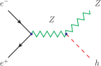
Figure 1: LO process: $e^{-}(p_{1})~{}+~{}e^{+}(p_{2})\rightarrow Z(k_{1})~{}+~{}h(k_{2})$

The expression for the matrix element squared has the following form:

$$\left|{\bf M}_{e^{+}e^{-}\rightarrow Zh}^{\mathrm{LO}}\right|^{2}=\frac{2e^{4}\left(g_{v}^{2}+g_{a}^{2}\right)}{s_{W}^{2}c_{W}^{2}}\cdot\frac{tu+2sM_{Z}^{2}-M_{h}^{2}M_{Z}^{2}}{\left(s-M_{Z}^{2}\right)^{2}+M_{Z}^{2}\Gamma_{Z}^{2}},$$ (11)

where $s_{W}=\sin\theta_{W},~{}c_{W}=\cos\theta_{W}$ with $\theta_{W}$ the weak mixing angle, and

$$g_{v}=\frac{-1/2+2s_{W}^{2}}{2s_{W}c_{W}},~{}g_{a}=-\frac{1}{4s_{W}c_{W}}$$

are the vector and axial-vector couplings to to the $e^{+}e^{-}Z$ vertex, respectively. The Mandelstam variables are defined as

$$\left(p_{1}+p_{2}\right)^{2}=\left(k_{1}+k_{2}\right)^{2}=s,\,\left(p_{1}-k_{1}\right)^{2}=\left(p_{2}-k_{2}\right)^{2}=t,\,\left(p_{1}-k_{2}\right)^{2}=\left(p_{2}-k_{1}\right)^{2}=u,$$

and the relation $s+t+u=M_{Z}^{2}+M_{h}^{2}$. The total cross section reads

$$\sigma=\frac{1}{4}\frac{1}{48\pi s^{2}}\frac{e^{4}\left(g_{v}^{2}+g_{a}^{2}\right)}{s_{W}^{2}c_{W}^{2}}\cdot\frac{\left[\kappa\left(s,M_{Z}^{2},M_{h}^{2}\right)+12sM_{Z}^{2}\right]\kappa\left(s,M_{Z}^{2},M_{h}^{2}\right)}{\left(s-M_{Z}^{2}\right)^{2}+M_{Z}^{2}\Gamma_{Z}^{2}},$$ (12)

where the front $\frac{1}{4}$ is the spin average over the initial states, and the function $\kappa$ takes the form:

$$\kappa\left(x,y,z\right)=\sqrt{x^{2}+y^{2}+z^{2}-2xy-2xz-2yz}.$$

In general one loop corrections to the $e^{+}e^{-}\rightarrow Zh$ process shown in Fig. 2 consist of vertex corrections to the initial and finial vertex, self energy corrections to the mediated propagator, and box corrections with virtual particles in loop in contact with both initial and final states, respectively. The interaction between the extended scalars and initial fermions is negligible due to its suppressed Yukawa couplings of $\mathcal{O}\left(\frac{m_{f}}{M_{W}}\right)$. Therefore, in what follows, the NLO contribution originated from extended scalar loop corrections to the $Zh$ production consists of self energy and vertex corrections to the vector and scalar bosons, as indicated in Fig. 2 for the diagrams with hatching blobs.

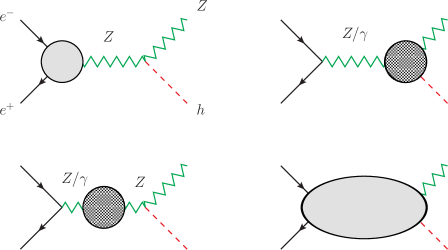
Figure 2: General one loop contributions to $e^{+}e^{-}\rightarrow Zh$ amplitude. The blobs denote one loop irreducible diagrams, and these hatched indicate where the extended scalar loop corrections can take place.

Loop corrections alone are often UV divergent and need be renormalized in certain renormalization scheme. We use dimensional regularization in $d=4-2\epsilon$ spacetime dimensions and the modified minimal subtraction ($\overline{\mathrm{MS}}$) scheme to perform the calculation. Here, we use the terms with caret $~{}\hat{}~{}$ denote the renormalized quantities, which are the bare quantities subtracting the part proportional to $\frac{1}{\bar{\epsilon}}=\frac{1}{\epsilon}-\gamma_{E}+\log 4\pi$ by definition. In this scheme, the one loop amplitude can be written as below

$$i{\bf M}_{e^{+}e^{-}\rightarrow Zh}^{\mathrm{NLO}} =i{\bf M}_{e^{+}e^{-}\rightarrow Zh}^{\mathrm{tree}}+i{\bf M}_{e^{+}e^{-}\rightarrow Zh}^{\mathrm{self}}+i{\bf M}_{e^{+}e^{-}\rightarrow Zh}^{\mathrm{vert}},$$ (13)

$$=-i\frac{\hat{e}^{2}\hat{M}_{Z}}{\hat{s}\hat{c}}\hat{\rho}_{NC}\left(s\right)\bar{v}\left(p_{2}\right)\gamma^{\mu}\left(g_{v}^{eff}-g_{a}^{eff}\gamma_{5}\right)u\left(p_{1}\right)\epsilon_{\mu}\left(k_{1}\right)+i{\bf M}_{Z^{*}\rightarrow Zh}^{\mathrm{vert}}+i{\bf M}_{\gamma^{*}\rightarrow Zh}^{\mathrm{vert}},$$

where the last two terms on the right hand side denote the contribution of $ZZh$ and $\gamma Zh$ vertex corrections, and $\hat{s},\hat{c}$ are sine and cosine of the weak mixing angle at 1-loop level in $\overline{\mathrm{MS}}$ scheme and can be expressed in terms of the $\overline{\mathrm{MS}}$ masses such that $\hat{c}^{2}=1-\hat{s}^{2}=\hat{M}_{W}^{2}/\hat{M}_{Z}^{2}$. The effective vector and axial-vector coupling $g_{v}^{eff},g_{a}^{eff}$ have the following form

$$g_{v}^{eff}=\frac{I_{W,e}^{3}-2\hat{\kappa}\left(s\right)\hat{s}^{2}Q_{e}}{2\hat{s}\hat{c}},\quad g_{a}^{eff}=\frac{I_{W,e}^{3}}{2\hat{s}\hat{c}},$$ (14)

where the factor $\hat{\kappa}\left(s\right)$ modifying $\hat{s}^{2}$ originates from the $\gamma-Z$ mixing tensor and

$$\hat{\kappa}\left(s\right)=1-\frac{\hat{c}}{\hat{s}}\frac{\hat{\Sigma}_{T}^{\gamma Z}\left(s\right)}{s}.$$

The factor $\hat{\rho}_{NC}\left(s\right)$ takes the form

$$\hat{\rho}_{NC}\left(s\right)= \frac{1}{s-\hat{M}_{Z}^{2}+\hat{\Sigma}_{T}^{ZZ}\left(s\right)}\left(1+\frac{1}{2}\delta\hat{Z}_{ZZ}+\frac{1}{2}\delta\hat{Z}_{h}\right),$$ (15)

$$= \frac{1}{s-M_{Z}^{2}+i\Gamma_{Z}M_{Z}}\left(1+\frac{\mathrm{Re}\hat{\Sigma}_{T}^{ZZ}\left(M_{Z}^{2}\right)-\mathrm{Re}\hat{\Sigma}_{T}^{ZZ}\left(s\right)}{s-M_{Z}^{2}}+\frac{1}{2}\delta\hat{Z}_{ZZ}+\frac{1}{2}\delta\hat{Z}_{h}\right)$$

$$+\mathcal{O}\left(\alpha^{2},\frac{\Gamma_{Z}^{2}}{M_{Z}^{2}}\right)$$

where we expand the expression in the second(third) line and omit terms of $\mathcal{O}\left(\alpha^{2}\right)$ or $\mathcal{O}\left(\frac{\Gamma_{Z}^{2}}{M_{Z}^{2}}\right)$ using

$$\hat{M}_{Z}^{2}=M_{Z}^{2}+\mathrm{Re}\hat{\Sigma}_{T}^{ZZ}\left(M_{Z}^{2}\right),\quad\Gamma_{Z}M_{Z}=\mathrm{Im}\hat{\Sigma}_{T}^{ZZ}\left(s\right),$$

and

$$\delta\hat{Z}_{ZZ}=\hat{Z}_{ZZ}-1=-\mathrm{Re}\left.\frac{\partial\hat{\Sigma}_{T}^{ZZ}\left(k^{2}\right)}{\partial k^{2}}\right|_{k^{2}=M_{Z}^{2}},\quad\delta\hat{Z}_{h}=\hat{Z}_{h}-1=-\mathrm{Re}\left.\frac{\partial\hat{\Sigma}^{h}\left(k^{2}\right)}{\partial k^{2}}\right|_{k^{2}=M_{h}^{2}},$$

with $\hat{Z}_{ZZ},~{}\hat{Z}_{h}$ the finite residues of $Z$ and $h$ propagators. The self energy functions in all scalar multiplet models that are relevant in our calculation are listed in Appendix C.2.

We separate the vertex corrections in Eq. (13) because they cannot fully factorize to Born (extra Lorentz structures other than that of the LO amplitude). It should be noted that the vertex corrections alone are free of UV divergences, and thus can be written individually apart from the Born-like structure. Therefore, the total NLO corrections at matrix element square level can be obtained as below

$$\left|{\bf M}\right|_{\mathrm{tot,corr}}^{2}=\left|{\bf M}_{e^{+}e^{-}\rightarrow Zh}^{\mathrm{NLO}}\right|^{2}-\left|{\bf M}_{e^{+}e^{-}\rightarrow Zh}^{\mathrm{LO}}\right|^{2},$$ (16)

where ${\bf M}_{e^{+}e^{-}\rightarrow Zh}^{\mathrm{LO}}$ is the amplitude at the leading order. And the amplitude square of ${\bf M}_{e^{+}e^{-}\rightarrow Zh}^{\mathrm{NLO}}$ is

$$\left|{\bf M}_{e^{+}e^{-}\rightarrow Zh}^{\mathrm{NLO}}\right|^{2}=\frac{\hat{e}^{4}\hat{M}_{Z}^{2}\left(g_{v,eff}^{2}+g_{a,eff}^{2}\right)}{M_{Z}^{2}\hat{s}^{2}\hat{c}^{2}}\left|\hat{\rho}_{NC}\right|^{2}\left(tu+2sM_{Z}^{2}-M_{h}^{2}M_{Z}^{2}\right)+\ldots,$$ (17)

where the ellipsis denotes other contributions that are at NLO and NNLO level. For the NLO contribution it is contained in the interference between the vertex term and the first term in the last line of Eq. (13) and in particular the exact NLO level contribution reads

$$2~{}\mathrm{Re}\left[\left({\bf M}_{Z^{*}\rightarrow Zh}^{\mathrm{vert}}+{\bf M}_{\gamma^{*}\rightarrow Zh}^{\mathrm{vert}}\right)\cdot\left({\bf M}_{e^{+}e^{-}\rightarrow Zh}^{\mathrm{tree}}\right)^{*}\right]$$ (18)

$$= -\frac{1}{16\pi^{2}}\frac{4~{}e^{3}}{M_{Z}s_{W}c_{W}}\sum_{s,\left(M_{1},M_{2}\right)}\left(\frac{g_{ssh}g_{ssZ}^{2}\left(g_{v}^{2}+g_{a}^{2}\right)}{\left(s-M_{Z}^{2}\right)^{2}+M_{Z}^{2}\Gamma_{Z}^{2}}+\frac{g_{ssh}g_{ss\gamma}g_{ssZ}~{}g_{v}\left(s-M_{Z}^{2}\right)}{s\left[\left(s-M_{Z}^{2}\right)^{2}+M_{Z}^{2}\Gamma_{Z}^{2}\right]}\right)\times$$

$$2\mathrm{Re}\Bigg{\{}\left(tu+2sM_{Z}^{2}-M_{h}^{2}M_{Z}^{2}\right)\left(2C_{24s}\left(M_{1},M_{2}\right)-\frac{1}{2}B_{0}\left(k_{2},M_{2},M_{2}\right)\right)$$

$$+\left(s+M_{Z}^{2}-M_{h}^{2}\right)\left(M_{h}^{2}M_{Z}^{2}-tu\right)\left(C_{22s}\left(M_{1},M_{2}\right)-C_{23s}\left(M_{1},M_{2}\right)\right)\Bigg{\}},$$

where the expressions of $C_{22s}\left(M_{1},M_{2}\right)$, $C_{23s}\left(M_{1},M_{2}\right)$ and $C_{24s}\left(M_{1},M_{2}\right)$ can be found in Appendix C.3, and $\sum_{s,\left(M_{1},M_{2}\right)}$ denotes the sum of all possible scalar couplings and corresponding pair of scalar masses $\left(M_{1},M_{2}\right)$. $g_{ssh},~{}g_{ssZ},~{}g_{ss\gamma}$ are the couplings of scalar-scalar-Higgs, scalar-scalar-$Z$ and scalar-scalar-photon, respectively. The Feynman rules of the multiplets in the gauge coupling sector can be found in Appendix A. The masses in the pair $\left(M_{1},M_{2}\right)$ are degenerate ($M_{1}=M_{2}$) in all scalar models for each induced scalar triangle loop except for that in the inert doublet model which has the two masses assigned differently.

4 Numerical Results in $\overline{\mathrm{MS}}$ Scheme

In this section, we present the contour comparison between relative corrections to $Zh$ production and the Higgs diphoton ($h\gamma\gamma$) decay rate induced by scalar multiplet loop contributions, with an effort to delineate the prospective BSM parameter space constraints implied by each process. The relative correction by the scalar-induced loop contribution to the $e^{+}e^{-}\rightarrow Zh$ process is defined as follows,

$$\delta\sigma_{Zh}=\frac{\sigma_{\mathrm{BSM}}^{\mathrm{1-loop}}}{\sigma_{\mathrm{SM}}^{\mathrm{LO}}},$$ (19)

where $\sigma_{\mathrm{BSM}}^{\mathrm{1-loop}}$ is the total cross section based on the matrix element square term in Eq. (16), and $\sigma_{\mathrm{SM}}^{\mathrm{LO}}$ is the LO total cross section given in Eq. (12). There are three commonly-used input-parameter schemes for the calculation of EW radiative corrections: the $\alpha\left(0\right)$, $\alpha\left(M_{Z}\right)$ and $G_{\mu}$ schemes, respectively. All are suited for both the $\overline{\mathrm{MS}}$ and OS renormalization schemes. Each scheme has its advantages and disadvantages. The most suitable choice depends on the nature of process under consideration. In general, the $\alpha\left(M_{Z}\right)$ and $G_{\mu}$ schemes render the SM EW corrections free of explicit large logarithms involving light fermion masses and are, therefore, preferable over the $\alpha\left(0\right)$ scheme if no external photons are involved in the process. A detailed discussion of these input-parameter schemes as well as the relation between one another can be found in Ref. Denner:2019vbn . In the present context, the one-loop contribution from the extended scalar sector particles in our study can be performed independently of the overall SM EW contribution, and the result is manifestly free from light fermion mass logarithms. Moreover, the impact on $\sigma(e^{+}e^{-}\to Zh)$ of the renormalized extended scalar sector loop contribution is less sensitive to the choice of input parameter scheme than is the SM one-loop contribution. Hence, for simplicity we use the $\alpha\left(0\right)$ input-parameter scheme and set the corresponding SM input parameters as follows:

$$\alpha^{-1}=\left(\frac{e^{2}}{4\pi}\right)^{-1}=137.036,$$ (20)

$$M_{W}=80.385~{}\mathrm{GeV},~{}M_{Z}=91.1876~{}\mathrm{GeV},~{}\Gamma_{Z}=2.4952~{}\mathrm{GeV},~{}M_{h}=125.1~{}\mathrm{GeV}.$$

At one-loop level in $\overline{\mathrm{MS}}$ scheme the vector boson masses ($M_{V},~{}\left(V=W,Z\right)$), mixing angle ($\hat{s},\hat{c}$) and the electric charge ($\hat{e}$) are

$$\hat{M}_{V}^{2}=M_{V}^{2}+\mathrm{Re}\hat{\Sigma}_{T}^{VV}\left(M_{V}^{2}\right),$$ (21)

$$\hat{c}^{2}=1-\hat{s}^{2}=\frac{\hat{M}_{W}^{2}}{\hat{M}_{Z}^{2}},$$

$$\hat{e}=e\left(1-\frac{1}{2}\delta\hat{Z}_{\gamma\gamma}-\frac{1}{2}\frac{\hat{s}}{\hat{c}}\delta\hat{Z}_{Z\gamma}\right),$$

where the expressions of $\delta\hat{Z}_{\gamma\gamma},~{}\delta\hat{Z}_{Z\gamma}$ can be found in Eq. (84) and the self energy functions are given in Appendix C.2.

Turning now to the $h\to\gamma\gamma$ process, the relative correction by scalar-induced loop contributions to the Higgs diphoton decay rate is defined below

$$\delta R_{h\gamma\gamma}=\frac{\Gamma^{\mathrm{BSM}+\mathrm{SM}}_{h\rightarrow\gamma\gamma}-\Gamma^{\mathrm{SM}}_{h\rightarrow\gamma\gamma}}{\Gamma^{\mathrm{SM}}_{h\rightarrow\gamma\gamma}},$$ (22)

where the expression of Higgs diphoton decay width is given by,

$$\Gamma^{\mathrm{BSM}+\mathrm{SM}}_{h\rightarrow\gamma\gamma}= \frac{G_{F}\alpha^{2}M_{h}^{3}}{128\sqrt{2}\pi^{3}}\left|\sum_{f}N_{c}Q_{f}^{2}g_{hff}A_{1/2}^{h}\left(\tau_{f}\right)+g_{hWW}A_{f}^{h}\left(\tau_{W}\right)-\sum_{s}\frac{M_{W}}{g_{2}M_{s}^{2}}g_{ss\gamma}^{2}g_{ssh}A_{0}^{h}\left(\tau_{s}\right)\right|^{2},$$ (23)

with the loop functions $A_{1/2}^{h},~{}A_{1}^{h},~{}A_{0}^{h}$ defined as Djouadi:2005gj

$$A_{1/2}^{h}\left(\tau_{i}\right) =-2\tau_{i}\left[1+\left(1-\tau_{i}\right)\mathcal{F}\left(\tau_{i}\right)\right]$$ (24)

$$A_{1}^{h}\left(\tau_{i}\right) =2+3\tau_{i}+3\tau_{i}\left(2-\tau_{i}\right)\mathcal{F}\left(\tau_{i}\right)$$

$$A_{0}^{h}\left(\tau_{i}\right) =-\tau_{i}\left[1-\tau_{i}\mathcal{F}\left(\tau_{i}\right)\right],$$

and the function $\mathcal{F}\left(\tau_{i}\right)$ reads

$$\mathcal{F}\left(\tau_{i}\right)=\left\{\begin{array}[]{ll}\left[\sin^{-1}\left(\sqrt{\frac{1}{\tau_{i}}}\right)\right]^{2},&\tau_{i}\geq 1;\\ -\frac{1}{4}\left[\ln\left(\frac{1+\sqrt{1-\tau_{i}}}{1-\sqrt{1-\tau_{i}}}\right)-i\pi\right]^{2},&\tau_{i}<1;\end{array}\right.$$

and $\tau_{i}=4M_{i}^{2}/M_{h}^{2}~{}\left(i=f,W,s\right)$. $\Gamma^{\mathrm{SM}}_{h\rightarrow\gamma\gamma}$ shares the same expression with $\Gamma^{\mathrm{BSM}+\mathrm{SM}}_{h\rightarrow\gamma\gamma}$ but the last term in the module square in Eq. (23). One can see that only charged scalars contribute to the last term in Eq. (23) since $g_{ss\gamma}$ vanishes for neutral scalars.

Table 1 shows the estimated precision for $\sigma(Zh)$ production and $h\gamma\gamma$ decay signal rate for the CEPC and FCC-ee at $\sqrt{s}=240$ GeV as well as the ILC at $\sqrt{s}=250$ GeV. Note that all three exhibit roughly the same level of precision for $\sigma(Zh)$ measurements. Besides, the uncertainty on the measurement of the Higgs production via gluon and $b\bar{b}$ fusion in $h\to\gamma\gamma$ decay channel at the HL-LHC is also listed in the right end column in the table, whose precision is a few percent and somewhat better than those estimated in the future Higgs factories even though the $\sigma\left(Zh\right)$ measurement is much less precise. In what follows, provide numerical results assuming the CEPC projections CEPCStudyGroup:2018ghi for purposes of concrete illustration . In the following, we categorize our result into two cases where the constraints on the BSM parameter space by the $Zh$ production are complementary and degenerate to that by the Higgs diphoton decay rate, respectively. We assume the constraints on the quartic Higgs (portal) couplings from the perturbativity in each model are subject to the relation

$$\lambda_{i}\left(\mu\right)\lesssim\frac{\lambda_{\text{FP}}}{3},$$ (25)

where $\lambda_{\text{FP}}=12.1\ldots$ is the value at a fixed point where $\beta_{\lambda}=0$ . The renormalization scale $\mu\in\left[M_{Z},\Lambda\right]$, and $\Lambda$ is the cutoff scale of the theory. This relation is an extension to the approximate perturbativity constraint on the couplings in the complex singlet model in Ref. Gonderinger:2012rd which is based on the work in Ref. Riesselmann:1996is .

Table 1: Estimated precision of CEPC, FCC-ee and ILC for $\sigma(Zh)$ and $h\to\gamma\gamma$ signal rate. The projected precision for the CEPC and FCC-ee are taken from Refs. CEPCStudyGroup:2018ghi ; Abada:2019lih and those for the ILC are from Table 3 in Ref. Durieux:2017rsg , which are rescaled from the luminosity samples of 250 fb^-1 in the ILC operating Scenarios Barklow:2015tja ; Bambade:2019fyw ; Fujii:2019zll . All quoted values are are for statistical uncertainties at the 68% confidence level. The total uncertainty (stat + syst) on the measurement for $h\to\gamma\gamma$ with Higgs production via gluon and $b\bar{b}$ fusion at the HL-LHC Cepeda:2019klc is listed in the last column on the right in comparison of that at the CEPC, FCC-ee and ILC.

Measurement	CEPC	FCC-ee	ILC	HL-LHC
	(240 GeV, 5.6 ab-1)	(240 GeV, 5 ab-1)	(250 GeV, 2 ab-1)	(14 TeV, 3 ab-1)
$\sigma\left(Zh\right)$	$0.50\%$	$0.50\%$	$0.71\%$	–
$\sigma\times\mathrm{BR}\left(h\rightarrow\gamma\gamma\right)$	$6.8\%$	$9.0\%$	$12\%$	$4\%$ (ggF+bbH)

It is worth mentioning that in order to verify that our result is independent of scheme choice, we also perform the one-loop calculation in an alternative renormalization scheme - on-shell renormalization scheme and obtain the consistent result with that in $\overline{\mathrm{MS}}$ scheme. One can refer to Appendix D for a detailed procedure of on-shell renormalization scheme.

4.1 Complementary with Higgs Diphoton Decays

Complex Triplet

The complex scalar triplet model with the hypercharge of the extended scalar triplet $Y=2$ is a component of the type-II seesaw model Konetschny:1977bn ; Magg:1980ut ; Schechter:1980gr ; Cheng:1980qt . The neutrino masses are obtained through the Yukawa interaction term in the type-II seesaw model below

$$\mathcal{L}_{\text{Yuk}}=h_{ij}\overline{L^{Ci}}i\tau_{2}\Delta L^{j}+\text{h.c.},$$ (26)

where $h_{ij}$ is the neutrino Yukawa coupling that is complex and symmetric, $L_{i}=\left(\nu_{i},e_{i}\right)_{L}^{T}$ $\left(i=e,\mu,\tau\right)$ is a left-handed lepton doublet, and $\Delta$ is a $2\times 2$ representation of the complex triplet fields (see expression below (66)). After electroweak symmetry breaking (EWSB), the neutrinos acquire masses due to non-vanishing triplet vacuum expectation value (VEV) $v_{\Delta}\neq 0$, and the neutrino mass matrix reads

$$m_{\nu,ij}=\sqrt{2}h_{ij}v_{\Delta}.$$ (27)

Meanwhile the minimization of the potential (66) gives rise to the triplet VEV

$$v_{\Delta}\approx\frac{\mu v_{\phi}^{2}}{\sqrt{2}\left[M^{2}+\frac{\lambda_{4}+\lambda_{5}}{2}v_{\phi}^{2}\right]},$$ (28)

when $v_{\Delta}/v_{\phi}\ll 1$. One can see that for fixed $\lambda_{4},\lambda_{5}$, $v_{\Delta}\rightarrow 0$ with $M/v_{\phi}\gg 1$. Being constrained by the $\rho$ parameter the upper bound of the triplet VEV $v_{\Delta}\lesssim 3~{}\mathrm{GeV}$ Du:2018eaw , so that the sine of the mixing angles  are highly suppressed since $\propto v_{\Delta}/v_{\phi}\ll 1$. Therefore, in what follows, we consider the scalar triplet unmixed with the SM Higgs doublet after EWSB, as being treated in the other models with zero VEV in the subsequent subsection.

We observe that the complex triplet makes the most interesting case in our study, as it exhibits the complementary sensitivity between the $Zh$ and $h\gamma\gamma$ decay rate precision measurements. In this model, there are three free parameters that enter the one-loop calculation, which are $\lambda_{4},~{}\lambda_{5}$ and $M_{\Delta}$, respectively. The scalar triplet masses are given by

$$M_{H^{\pm\pm}}^{2} =M_{\Delta}^{2}-\frac{\lambda_{5}v_{\phi}^{2}}{2},$$ (29)

$$M_{H^{\pm}}^{2} =M_{\Delta}^{2}-\frac{\lambda_{5}v_{\phi}^{2}}{4},$$

$$M_{H}^{2} =M_{A}^{2}=M_{\Delta}^{2},$$

with $M_{H^{\pm\pm}}$, $M_{H^{\pm}}$, $M_{H}$ and $M_{A}$ the masses of the doubly and singly charged, CP-even and CP-odd neutral scalar, respectively. In Fig. 3 the contours of $\left|\delta\sigma_{Zh}\right|\leq 0.5\%$ ($1\sigma$ cyan band with dashed central and outer lines) and $\left|\delta R_{h\gamma\gamma}\right|\leq 6.8\%$ ($1\sigma$ orange band with solid central and outer lines) are plotted in $\left(\lambda_{4},\lambda_{5}\right)$ plane with $M_{\Delta}=400,~{}800~{}\mathrm{GeV}$. To illustrate a straightforward improvement for probing region of parameter space in Higgs diphoton decay channel when increasing the precision for the measurement in this channel, a contour of $\left|\delta R_{h\gamma\gamma}\right|\leq 4\%$ ($1\sigma$ grey band with dashdotted central and outer lines) corresponding to the precision at the HL-LHC is also plotted. A shrinking of the band width constraining parameter $\lambda_{4}$ is apparent with smaller uncertainties on the Higgs diphoton decay measurement.

The ellipse encompassing the crossed range between the two bands on each plot outlines the constraints of the parameter $\lambda_{4}$ and $\lambda_{5}$ at $95\%$ confidence level when combining $\left|\delta\sigma_{Zh}\right|\leq 0.5\%$ and $\left|\delta R_{h\gamma\gamma}\right|\leq 6.8\%$ and using $\chi^{2}$ test for 2 degree-of-freedom. One can see a cross-like shape for the two contours, indicating complementary results between the two processes and thereby putting the most stringent constraints one another. We find that as the mass of the neutral component ($M_{\Delta}$) increases the cyan band (with dashed lines) as the contour from $\left|\delta\sigma_{Zh}\right|\leq 0.5\%$ gets flatter and becomes less dependent of the parameter $\lambda_{4}$ . This can be explained as follows. As one can see in Eq. (29) the mass difference of differently charged components is proportional to $\lambda_{5}$. Performing the large mass expansion in the range of $s/M_{\Delta}^{2}\ll 1$ to the self energy and vertex loop functions, we find that the dominant contribution is from the $WW$ self energy contribution that enters $\hat{s}$ and $\hat{c}$ (see first and second lines in Eq. (21)) due to the mass splitting between scalars with different number of charges and the mass difference is solely proportional to $\lambda_{5}$ (see expression of $\Sigma_{T}^{WW}\left(k^{2}\right)$ in (79) and apply large mass expansion to $B_{0}$ functions). On the other hand, as for the orange band, when neglecting the mass difference in the loop function $A_{0}^{h}\left(\tau_{i}\right)$ (which is valid in the large mass limit as the case we discuss above using large mass expansion), the minimization of the $\delta R_{h\gamma\gamma}$ (i.e., the third term in the modular square in Eq. (23) vanishes) gives rise to a simple linear relation between $\lambda_{4}$ and $\lambda_{5}$ that $10\lambda_{4}+\lambda_{5}=0$, which roughly reflects the central position of the orange band in Fig. 3. In other words, the complementary parameter space probes by the precision measurement for $\sigma\left(Zh\right)$ and $h\to\gamma\gamma$ decay rate are realized in two aspects:

1. The BSM contribution to $\sigma\left(Zh\right)$ is dominated by the $WW$ self energy via differently charged scalar in loops which is susceptible to the variation of the mass splitting parameter ($\lambda_{5}$), compared to other types of corrections.

2. The BSM contribution to $h\to\gamma\gamma$ decay rate involves triple Higgs couplings with two charged Higgs that have a stronger dependence on the parameter $\lambda_{4}$ than on the other couplings (see Feynman rules in Table 4), making it more susceptible to variation in $\lambda_{4}$.

Therefore, the complementarity is observed when exploring the parameter space in the plane $\left(\lambda_{4},\lambda_{5}\right)$. Furthermore, from the ellipses constraining the parameter $\lambda_{4}$ and $\lambda_{5}$ at $95\%$ confidence level one also can see that the constraint on $\lambda_{5}$ is stronger than that on $\lambda_{4}$ with increase of $M_{\Delta}$.

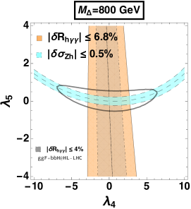
Figure 3: Contour comparison of $\left|\delta\sigma_{Zh}\right|\leq 0.5\%$ ($1\sigma$ cyan band with dashed central and outer lines) and $\left|\delta R_{h\gamma\gamma}\right|\leq 6.8\%$ ($1\sigma$ orange band with solid central and outer lines) in complex triplet model with $M_{\Delta}=400~{}\mathrm{GeV}$ (left) and $M_{\Delta}=800~{}\mathrm{GeV}$ (right), respectively. The ellipse on each plot denotes the $95\%$ confidence level for the parameter $\lambda_{4}$ and $\lambda_{5}$ with corresponding fixed $M_{\Delta}$. In addition, the contour of $\left|\delta R_{h\gamma\gamma}\right|\leq 4\%$ ($1\sigma$ grey band with dashdotted central and outer lines) corresponding to the accuracry at the HL-LHC via gluon and $b\bar{b}$ fusion is added for the comparison, where one can see that with higher precision on $h\to\gamma\gamma$ decay rate a better constraint on the parameter $\lambda_{4}$ can be archieved.

Instead of fixing the neutral scalar mass, one may fix one of the two coupling parameters and investigate the contours of $\delta\sigma_{Zh}$ and $\delta R_{h\gamma\gamma}$ at $1\sigma$ level in the neutral scalar mass and coupling parameter plane. First we can make slice of the contours in the $\left(M_{\Delta},\lambda_{5}\right)$ plane with fixed $\lambda_{4}$. Judging from Fig. 3, the boundary of $\lambda_{4}$ with $M_{\Delta}=400~{}\mathrm{GeV}$ is $\left|\lambda_{4}\right|\sim 1$ and that with $M_{\Delta}=800~{}\mathrm{GeV}$ is $\left|\lambda_{4}\right|\sim 3$ which are still within the allowed perturbativity range (25); while the constraint on parameter $\lambda_{5}$ keeps it in a small range $\left|\Delta\lambda_{5}\right|\lesssim 0.4$ ($\left|\lambda_{5}\right|\lesssim 0.2$ for small $\lambda_{4}$).

Fig. 4 shows the two contours of $\left|\delta\sigma_{Zh}\right|\leq 0.5\%$ and $\left|\delta R_{h\gamma\gamma}\right|\leq 6.8\%$ with the fixed $\lambda_{4}=1,~{}3$, respectively. The contour of $\left|\delta\sigma_{Zh}\right|\leq 0.5\%$ constantly restricts $\lambda_{5}$ within a thin strip region, while the contour of $\left|\delta R_{h\gamma\gamma}\right|\leq 6.8\%$ puts a lower bound $M_{\Delta}$ region, so that in the overlapping area of the two contours the lower bound of the mass $M_{\Delta}$ is approximately $400~{}\mathrm{GeV}$ for $\lambda_{4}=1$ and $800~{}\mathrm{GeV}$ for $\lambda_{4}=3$. Similar lower bound of $M_{\Delta}$ can be obtained for negative $\lambda_{4}$, i.e., $\lambda_{4}=-1,-3$, respectively. This is consistent with the result in Fig. 3, where the left figure ($M_{\Delta}=400~{}\mathrm{GeV}$) has the boundary of $\left|\lambda_{4}\right|\lesssim 1$ and the right figure ($M_{\Delta}=800~{}\mathrm{GeV}$) has the boundary of $\left|\lambda_{4}\right|\lesssim 3$.

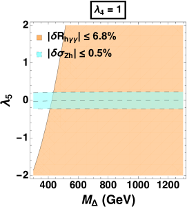
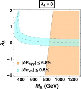
Figure 4: Contour comparison of $\left|\delta\sigma_{Zh}\right|\leq 0.5\%$ (cyan band outlined with dashed lines) and $\left|\delta R_{h\gamma\gamma}\right|\leq 6.8\%$ (orange area outlined with solid line) in complex triplet model in plane $\left(M_{\Delta},\lambda_{5}\right)$ with $\lambda_{4}=1$ (left) and $\lambda_{4}=3$ (right).

In addition to the constraints from perturbativity (25), vacuum stability and perturbative unitarity also impose boundaries in the parameter space. In general any of the above three sources of constraints impacts all the couplings in the potential. For instance, in Ref. Du:2018eaw it was shown that vacuum stability and perturbative unitarity at tree-level with fixed values of $\lambda_{2}=0.2$ and $\lambda_{3}=0$ require the parameter space in the $\left(\lambda_{4},\lambda_{5}\right)$ plane to be mostly in the 4th quadrant, and initial condition ($\lambda_{i}$ fixed at the starting scale) should be set first for the renormalization group equations (RGEs) to test the perturbativity with running scales, which are both illustrated in Fig. 1 therein. On the other hand, the constraints by the precision measurement on $Zh$ and $h\gamma\gamma$ decay rate only rely on the Higgs portal couplings $\left(\lambda_{4},\lambda_{5}\right)$ in addition to the triplet mass spectrum, which therefore, complement that by perturbativity, vacuum stability and perturbative unitarity.

As discussed above that the upper bound of the triplet VEV $v_{\Delta}\lesssim 3$ GeV is strictly constrained by the $\rho$ parameter and the sine of the mixing angles are highly suppressed so that one can consider the scalar triplet and the SM doublet fields do not mix together and treat the virtual scalar triplet loop corrections to the $Zh$ production separately. On the other hand, as can be seen in (27) that the neutrino masses derived from the type-II seesaw model depend on the neutrino Yukawa couplings $h_{ij}$ and the triplet VEV $v_{\Delta}$. The sum of neutrino masses has an upper bound, and in the context of a minimal 7-parameter model ($\mathrm{\Lambda CDM}+\sum m_{\nu}$) one obtains $\sum m_{\nu}<0.12$ eV (95%CL) from the combination of Planck 2018 and BAO Aghanim:2018eyx ; Zyla:2020zbs data sets. The parameters $h_{ij}$ and $v_{\Delta}$, however, are not individually rigorously constrained (e.g., $v_{\Delta}$ could be in the KeV or GeV regime), because their product yields the light neutrino mass matrix. For a fixed $v_{\Delta}$, a larger (smaller) $h_{ij}$ corresponds to a larger (smaller) value for neutrino masses, and vice versa.

As discussed in Ref. Du:2018eaw , this interplay of $h_{ij}$ and $v_{\Delta}$ affects the sensitivity of collider probes of the complex triplet model. At the LHC and a prospective 100 TeV $pp$ collider, the dominant discovery channels could be $H^{++}H^{--}$ and $H^{\pm\pm}H^{\mp}$ depending on the value of $v_{\Delta}$ Du:2018eaw . The doubly charged Higgs $H^{\pm\pm}$ could decay into same-sign di-leptons (di-bosons) and the branching ratio Br$\left(H^{\pm\pm}\to l^{\pm}l^{\pm}\right)$ (Br$\left(H^{\pm\pm}\to W^{\pm}W^{\pm}\right)$) depends on the parameters $M_{\Delta}$, $\lambda_{5}$, and $h_{ij}$ ($M_{\Delta}$, $\lambda_{5}$, and $v_{\Delta}$). The singly charged Higgs $H^{\pm}$ has the decay vertex $H^{\pm}hW^{\mp}$ and Br$\left(H^{\pm}\to hW^{\pm}\right)$ depends on the parameters $M_{\Delta}$, $\lambda_{4}$, $\lambda_{5}$ and $v_{\Delta}$. In Ref. Du:2018eaw the regions of $>5\sigma$ significance  are obtained using the discovery channels $H^{++}H^{--}$ and $H^{\pm\pm}H^{\mp}$ with $H^{\pm\pm}$ decaying into same-sign di-leptons and/or di-bosons in the $\left(M_{\Delta},v_{\Delta}\right)$ plane with fixed neutrino masses ($m_{\nu_{l}}=0.01$ eV for $l=e,\mu,\tau$) and Higgs portal couplings ($\lambda_{4}=0,\lambda_{5}=-0.1$) (see Fig. 7 therein).

In our study, we find that the parameter $\lambda_{5}$ could be tightly constrained ($\left|\Delta\lambda_{5}\right|\lesssim 0.4$) by the precision measurement for the $Zh$ cross section since $\sigma\left(Zh\right)$ is sensitive to the mass splitting between the scalar components. Moreover, measurements of $\sigma\left(Zh\right)$ and $\Gamma(H\to\gamma\gamma)$ provide complementary information, as illustrated in Fig. 4. The Higgs di-photon decay rate is relatively insensitive to $\lambda_{5}$ but strongly-dependent on $\lambda_{4}$. Therefore, with additional information about the Higgs portal parameters one might further delineate the discovery regions in the $\left(M_{\Delta},v_{\Delta}(h_{ij})\right)$ plane for given values of the neutrino masses.

To illustrate, we take two benchmark points from Ref. Du:2018eaw to show the consistency on the Higgs portal parameter space settings between the findings in our study and in probing the discovery channels with neutrino masses involved, which read

$$M_{\Delta}$$

400 & 800 GeV 91.1876 GeV 125 GeV 0.01 eV GeV 0.2 0 0 -0.1

We stress that the value of $M_{h}$ that is off 0.1 GeV compared to our settings in (20) ($125.1$ GeV for loop correction vs. $125$ GeV for the benchmark points) does not noticeably affect other settings. The mass of the neutrino is equal in the three generations. These two benchmark points represent two mass scales (low and high $M_{\Delta}$ region) and are covered by various overlapping discovery regions in the $\left(M_{\Delta},v_{\Delta}\right)$ plane (see Fig. 7 in Ref. Du:2018eaw ). In the analyses of Fig. 3 and Fig. 4 we already observe that with the choice of $M_{\Delta}=400~{}(800)~{}\mathrm{GeV}$, the regions of $\lambda_{4}$ and $\lambda_{5}$ constrained by the precision measurement of $Zh$ and $h\gamma\gamma$ decay rate approximate $\left|\lambda_{4}\right|\lesssim 1~{}(3)$ and $\left|\lambda_{5}\right|\lesssim 0.2$, which encompass $\left(\lambda_{4},\lambda_{5}\right)=\left(0,-0.1\right)$ for the two benchmark points in (4.1).

4.2 Degenerate with Higgs Diphoton Decay Sensitivity

In this subsection the models of interest including the inert doublet, real triplet, quintuplet and septuplet are studied, and likewise the constraints on the parameter space in each model are outlined in terms of the respective precision measurements on the $Zh$ production and Higgs diphoton decay rate. We find that in these models it gives less complementary sensitivity between the $Zh$ and Higgs diphoton decay rate precision measurement, showing (partial) degeneracy in constraining the parameter spaces between the $Zh$ and $h\gamma\gamma$ processes. In particular, there is a large degree of degeneracy on constraints of the parameter space between the two processes in the real triplet model; while in the inert doublet, quintuplet and septuplet models, since there are more free parameters it depends on which sliced parameter plane that one looks into to determine the degree of degeneracy.

Inert Doublet

The inert doublet model is the simplest two Higgs doublet model (THDM) that has an imposition of $\mathcal{Z}_{2}$ symmetry and therefore the lightest neutral component in the extended scalar sector could be a potential weakly interacting massive particle (WIMP) dark matter candidate . The extended scalar sector also decouple to the SM fermions due to its vanishing VEV. The interplay between the dark matter phenomenology and the EWPT in the context of the inert double model has been studied in a variety of spectra Borah:2012pu ; Gil:2012ya ; Blinov:2015vma ; Chowdhury:2011ga ; Cline:2013bln . It shows that a strongly first order electroweak phase transition (SFOEWPT) requires a large mass splitting between the dark matter candidate particle and the other extended scalars, and the Higgs funnel regime ($M_{H^{0}}\sim M_{h}/2$) is the only region of parameter space that can successfully saturate the dark matter abundance and provide a SFOEWPT Borah:2012pu ; Gil:2012ya ; Blinov:2015vma .

In the inert double model there are four free parameters that enter the one-loop calculation, which are $\{\mu_{2}^{2},~{}\lambda_{3},~{}\lambda_{4},~{}\lambda_{5}\}.$ The inert scalar masses are given by

$$M_{H^{\pm}}^{2} =\mu_{2}^{2}+\frac{1}{2}\lambda_{3}v_{\phi}^{2},$$ (30)

$$M_{H^{0}}^{2} =\mu_{2}^{2}+\frac{1}{2}\lambda_{L}v_{\phi}^{2},$$

$$M_{A^{0}}^{2} =\mu_{2}^{2}+\frac{1}{2}\lambda_{A}v_{\phi}^{2},$$

with $\lambda_{L,A}=\left(\lambda_{3}+\lambda_{4}\pm\lambda_{5}\right)$. Since only the charged component ($H^{\pm}$) contributes to the correction to the Higgs diphoton decay (refer to the last term on the right hand side of Eq. (23) where $g_{ss\gamma}\equiv 0$ for neutral scalars), it leaves us two parameters to plot the two contours of $\left|\delta\sigma_{Zh}\right|\leq 0.5\%$ and $\left|\delta R_{h\gamma\gamma}\right|\leq 6.8\%$ in the same plane, which are $\{\mu_{2},\lambda_{3}\}$. By fixing $\lambda_{4}$ and $\lambda_{5}$, Fig. 5 shows the two contours by $Zh$ and Higgs diphoton precision measurements in the $\left(\lambda_{3},M_{H^{\pm}}\right)$ plane, where $M_{H^{\pm}}$ is rescaled from $\mu_{2}$ according the first relation in Eq. 30. One can see that the contour by Higgs diphoton precision measurement is unchanged because it depends on no other parameters but $\lambda_{3}$ and $M_{H^{\pm}}\left(\mu_{2}\right)$. The contour by $Zh$ precision measurement is however dependent on the choice of parameters $\lambda_{4}$ and $\lambda_{5}$, as illustrated in Fig. 5. We find that compared to both vanishing $\lambda_{4}$ and $\lambda_{5}$ which makes a somewhat central-sit contour, the positive $\lambda_{4}$ pushes the contour downward and the negative upward, and non-vanishing $\lambda_{5}$ gives rise to higher lower boundary of $M_{H^{\pm}}$. Note that the sign of $\lambda_{5}$ alone does not change the shape of contour due to the fact that the two neutral components interchange the mass definition in Eq. (30) while the Feynman rules involving these two particles are identical (refer to the Feynman rule in Appendix A).

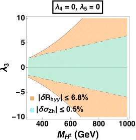
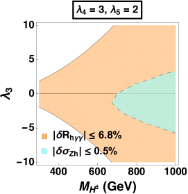
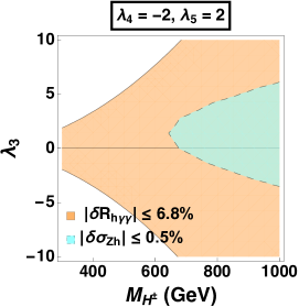
Figure 5: Contours in $\left(\lambda_{3},M_{H^{\pm}}\right)$ plane for $\left|\delta\sigma_{Zh}\right|\leq 0.5\%$ (cyan area outlined with dashed lines) and $\left|\delta R_{h\gamma\gamma}\right|\leq 6.8\%$ (orange area outlined with solid lines) in inert double model. From left to right panel, $\lambda_{4}$ and $\lambda_{5}$ are set at different values. The positive and negative $\lambda_{4}$ shifts the contour by $Zh$ precision measurement downward and upward accordingly. The non-zero $\lambda_{5}$ makes greater lower bound of $M_{H^{\pm}}$ compared to vanishing $\lambda_{5}$.

On the other hand, one observes that the inert scalars decouple from the Higgs diphoton process when setting $\lambda_{3}=0$ because $g_{H^{+}H^{-}h}\propto\lambda_{3}$. In the meantime, $\mu_{2}$ represents the mass of the physical charged Higgs $H^{\pm}$. In this case we consider the constraints of $\lambda_{4}$ and $\lambda_{5}$ by $Zh$ future precision are utterly complementary with that by Higgs diphoton future precision. Hence, one can plot the $Zh$ contours in $\{\lambda_{4},\lambda_{5}\}$ parameter space by fixing $\lambda_{3}=0$ and varying $M_{H^{\pm}}\left(\mu_{2}\right))$. Fig. 6 shows contours of $\left|\delta\sigma_{Zh}\right|\leq 0.5\%$ with $M_{H^{\pm}}=300,~{}500,~{}700~{},900~{}\mathrm{GeV}$ in the inert double model, where the area within the red dashed square denotes the perturbativity area of $\left(\lambda_{4},~{}\lambda_{5}\right)$ Hambye:1996wb . The contours of $\delta R_{h\gamma\gamma}$ is missing in this case due to $\delta R_{h\gamma\gamma}\equiv 0$ when $\lambda_{3}=0$.

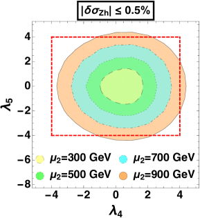
Figure 6: Contours in $\left(\lambda_{4},\lambda_{5}\right)$ plane for $\left|\delta\sigma_{Zh}\right|\leq 0.5\%$ in inert double model with $\mu_{2}=300,~{}500,~{}700,~{}900~{}\mathrm{GeV}$, which correspond to concentric areas in yellow, green, cyan and orange, and are respectively outlined with dashed, dotted, dash-dotted and solid lines. With the increase of $\mu_{2}$ the contour area gets larger and eventually excesses the region of perturbativity of the $\lambda$ parameters in the scalar potential. The allowed region of perturbativity is dictated within the red dashed box according to (25).

In order to see if the constraints on the parameters in our study give region of interest where the SFOEWPT occurs, we exploit the benchmark models (BMs) specified in Ref. Blinov:2015vma and mark the three benchmark points "BM1, BM2, BM3" corresponding to the three benchmark scenarios in the $\left(\lambda_{3},M_{H^{\pm}}\right)$ plane along with the contours by $h\gamma\gamma$ decay and $Zh$ precision measurement in Fig. 7. The legends "L1, L2, L3" on the right hand side of the figure denote the contours by $Zh$ precision measurement (i.e., $\left|\delta\sigma_{Zh}\right|\leq 0.5\%$) with the fixed $\lambda_{4}$ and $\lambda_{5}$ in accordance with that in "BM1, BM2, BM3", respectively. One can find the input parameters for the three benchmark scenarios in Table 2. As can be seen from Fig. 7, all three benchmark points are excluded from the contours by both the $h\gamma\gamma$ decay and $Zh$ precision measurement at 1-$\sigma$ confidence level. This tells us that with the expected CEPC precision the constrained parameter space may further exclude some region that has SFOEWPT and is permitted phenomenologically elsewhere like the benchmark scenarios used above.

Table 2: Input parameters for the three benchmark scenarios given in Ref.Blinov:2015vma . Masses are in unit $\mathrm{GeV}$. Couplings ($\lambda_{3},~{}\lambda_{4},~{}\lambda_{5}$) are valued at scale $Q=246~{}\mathrm{GeV}$ with finite temperature correction.

	$M_{H^{0}}$	$M_{A^{0}}$	$M_{H^{\pm}}$	$\lambda_{3}$	$\lambda_{4}$	$\lambda_{5}$
BM1	66	300	300	3.3	-1.7	-1.5
BM2	200	400	400	4.6	-2.3	-2.0
BM3	5	265	265	2.7	-1.4	-1.2

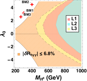
Figure 7: Contours in $\left(\lambda_{3},M_{H^{\pm}}\right)$ plane for $\left|\delta\sigma_{Zh}\right|\leq 0.5\%$ (red, cyan and yellow areas outlined with dotdashed, dotted and dashed lines and labelled with L1, L2 and L3) and $\left|\delta R_{h\gamma\gamma}\right|\leq 6.8\%$ (orange area outlined with solid lines). L1, L2 and L3 respectively denote the choice of $\lambda_{4}$ and $\lambda_{5}$ in accordance with that in BM1, BM2 and BM3, which are listed in Table 2. The three benchmark points BM1, BM2 and BM3 are marked with red crosses.

Real Triplet

The real triplet model has the extended scalar sector a real triplet with the neutral component a potential WIMP dark matter candidate if the triplet VEV is vanishing FileviezPerez:2008bj . Due to small mass splitting between the charged and neutral triplet scalars ($\Delta M=166~{}\mathrm{MeV}$) Cirelli:2005uq ; Cirelli:2007xd in the large scalar mass regime $M_{\Sigma}\gg M_{W}$, the direct search for the dark matter involves the process of charged scalar pair production accompanying the decay to neutral scalar and a soft $\pi^{\pm}$, the so-called disappearing charge tracks (DCTs). Experimentally, the DCT signature is profiled in search for the charginos at the LHC Aad:2013yna ; CMS:2014gxa ; Aaboud:2017mpt ; Sirunyan:2018ldc . The reach of the real triplet with DCT signature at the 13 TeV LHC and a possible future 100 TeV $pp$ collider is studied in Chiang:2020rcv . On the other hand, the Higgs portal parameter $\lambda_{3}$ may play a role in EWPT. The EWPT in the real triplet has been thoroughly studied in Niemi:2018asa ; Niemi:2020hto using dimensional reduction - a three dimensional effective field theory (DR3EFT) that allows non-perturbative lattice simulation.

In the real triplet model the free parameters from the potential that enter our calculation are the mass of the scalar triplet $M_{\Sigma}$ and $\lambda_{3}$, where we have omitted the mass splitting difference between the neutral and charged components at loop level since the splitting is small ($\Delta M=166~{}\mathrm{MeV}$ Cirelli:2005uq ; Cirelli:2007xd ) compared to the range of the mass investigated ($M_{\Sigma}\gtrsim 200~{}\mathrm{GeV}$). In this case, one has the contour plots in the parameter space $M_{\Sigma}$ versus $\lambda_{3}$ for both $\left|\delta\sigma_{Zh}\right|\leq 0.5\%$ and $\left|\delta R_{h\gamma\gamma}\right|\leq 6.8\%$ shown in Fig. 8, and can see that the contour by the $Zh$ measurement largely overlaps with that by the Higgs diphoton decay rate measurement. When $M_{\Sigma}\lesssim 400~{}\mathrm{GeV}$ the Higgs diphoton measurement reduces the positive bound of $\lambda_{3}$ while for the rest the $Zh$ measurement gives slight better constraints upon these two parameters. It is interesting to mention that the triplet dark matter direct search gives rise to much narrower window than the Higgs diphoton decay for $\lambda_{3}$ when $M_{\Sigma}$ is in $\mathrm{TeV}$ regime (see Figure 7 in Ref. Chiang:2020rcv ). Given the first order EWPT region provided in Niemi:2018asa ; Niemi:2020hto , one can compare this region with the constraints on the triplet mass $M_{\Sigma}$ and the Higgs portal coupling $\lambda_{3}$ by the precision measurement for $Zh$ production and $h\gamma\gamma$ decay rate at the CEPC to see in which area of the parameter space does it occur the first order EWPT, which is illustrated in Fig. 9, where the red strip represents the up-to-date first order EWPT region ($M_{\Sigma}\in[100,400]~{}\mathrm{GeV}$) calculated in Niemi:2020hto . As can be seen that with the CEPC required accuracy the first order EWPT could be excluded by precision measurement of the $h\gamma\gamma$ decay rate with $M_{\Sigma}\lesssim 350~{}\mathrm{GeV}$ while it is permitted in reference to the $Zh$ measurement solely.

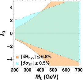
Figure 8: Contours in $\left(\lambda_{3},M_{\Sigma}\right)$ plane for $\left|\delta\sigma_{Zh}\right|\leq 0.5\%$ (cyan area outlined with dashed lines) and $\left|\delta R_{h\gamma\gamma}\right|\leq 6.8\%$ (orange area outlined with solid lines) in real triplet model.

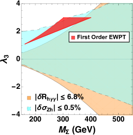
Figure 9: Contours same as that in Fig. 8 with superposition of the red region denoting the first order phase transition presented in Ref. Niemi:2020hto .

Quintuplet and Septuplet

The quintuplet and septuplet are the high dimensional EW scalar multiplets ($n=5,7$) carrying zero hypercharge ($Y=0$) so as to have the neutral components which could be potential WIMP dark matter candidates. The EW scalar multiplets of dimension $n$ are widely studied and discussed in Hambye:2009pw ; AbdusSalam:2013eya ; Chao:2018xwz ; Pilkington:2016erq . Ref. Chao:2018xwz updated the most general renormalizable potentials reported in previous studies Hambye:2009pw ; AbdusSalam:2013eya , and focused on $n=5,7$ cases to illustrate the dark matter phenomenology. In what follows, we follow the representation of the $\mathrm{SU\left(2\right)_{L}}$ EW scalar multiplet and the convention of the formulism adopted in Ref. Chao:2018xwz .

The quintuplet and septuplet have the same parameters that appear in the one-loop calculation and the difference is the fold of the scalar components respectively being $n=5$ and $n=7$. The scalar masses are given by

$$M_{S_{A}}^{2}=M_{A}^{2}+\frac{1}{2}\lambda_{1}v^{2}+\frac{2}{\sqrt{n}}M_{B}^{2}+\frac{1}{\sqrt{n}}\lambda_{3}v^{2},$$ (31)

$$M_{S_{B}}^{2}=M_{A}^{2}+\frac{1}{2}\lambda_{1}v^{2}-\frac{2}{\sqrt{n}}M_{B}^{2}-\frac{1}{\sqrt{n}}\lambda_{3}v^{2},$$

where the subscripts $A,~{}B$ denote the type of the scalars, and the mass of each type is equal regardless of the number of charges carried at tree level. Analogous to that in the real triplet model the radiative correction gives rise to small mass splitting between the charged and neutral component when $M_{S_{A,B}}\gg M_{W}$ that $M_{S_{A,B}^{m}}-M_{S_{A,B}^{0}}=m^{2}\Delta M$ ($m=-\frac{n-1}{2},\ldots,\frac{n-1}{2}$, $\Delta M=166~{}\mathrm{MeV}$ Cirelli:2005uq ; Cirelli:2007xd ). There are four free parameters from the potential that enter our calculation. They are the couplings $\lambda_{1},~{}\lambda_{3}$ and the masses either the unphysical $M_{A},~{}M_{B}$ or the physical $M_{S_{A}},~{}M_{S_{B}}$.

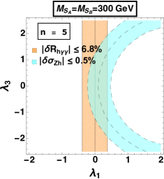
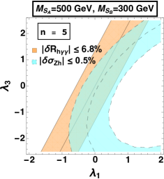
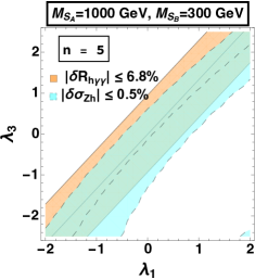
(a) Quintuplet

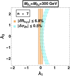
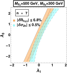
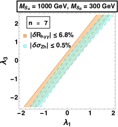
(b) Septuplet

Figure 10: Contour comparison for $\left|\delta\sigma_{Zh}\right|\leq 0.5\%$ (cyan band outlined with dashed lines) and $\left|\delta R_{h\gamma\gamma}\right|\leq 6.8\%$ (orange band outlined with solid lines) for quintuplet and septuplet with fixed values of the physical masses $\left(M_{S_{A}},~{}M_{S_{B}}\right)=\left(300,300\right),~{}\left(500,300\right),~{}\left(1000,300\right)~{}\mathrm{GeV}$, respectively.

We choose the physical masses $\left(M_{S_{A}},M_{S_{B}}\right)$ to be fixed and perform the contour comparison for the two processes in the $n=5,~{}7$ scalar model. Fig. 10 illustrates the comparisons with three sets of fixed $\left(M_{S_{A}},M_{S_{B}}\right)$. As we can see that the overlapping area varies with the setting of $\left(M_{S_{A}},M_{S_{B}}\right)$, and the two contours become more degenerate as increases of the mass difference between the type A and type B scalars. When the two physical masses are set to be equal, one observes that the $h\gamma\gamma$ decay rate constraint appears as a thin straight vertical band in the $\left(\lambda_{1},\lambda_{3}\right)$ plane, meaning the result is independent of the parameter $\lambda_{3}$. This is due to the natural of the tri-couplings $g_{s_{i}^{m}s_{i}^{-m}\gamma}$ and $g_{s_{i}^{m}s_{i}^{-m}h}$ ($i=A,~{}B$, the tri-couplings correspond to notation of vertices in Table 3 and 4 in Appendix A), which have the form

$$g_{S_{i}^{m}S_{i}^{-m}\gamma}=-em,\quad g_{S_{A}^{m}S_{A}^{-m}h}=-\left(\lambda_{1}+\frac{2}{\sqrt{n}}\lambda_{3}\right),\quad g_{S_{B}^{m}S_{B}^{-m}h}=-\left(\lambda_{1}-\frac{2}{\sqrt{n}}\lambda_{3}\right),$$ (32)

with $m=0,\ldots,\frac{n-1}{2}$. When $M_{S_{A}}=M_{S_{B}}$, the loop function $A_{0}^{h}\left(\tau_{s}\right)$ in Eq. (23) and (24) returns the same value for both $S_{A}$ and $S_{B}$, then the sum of the same charged components makes the exact cancellation of $\lambda_{3}$ between type $A$ and $B$ scalars.

In Ref. Chao:2018xwz it was found that the effective coupling is rather small $\left|\lambda_{\text{eff}}\right|\ll 1$ when saturating the observed relic density and evading the direct detection limits by LUX Akerib:2016vxi , PandaX-II Cui:2017nnn and XENONT1 Aprile:2018dbl . The effective coupling $\lambda_{\text{eff}}$ is a linear combination of parameter $\lambda_{1}$ and $\lambda_{3}$. One could take the septuplet for illustration to determine the constraints on the parameter space in connection with the dark matter phenomenology. The effective coupling in accord with our definition for the septuplet reads

$$\lambda_{\text{eff}}=\lambda_{1}-\frac{2}{\sqrt{7}}\lambda_{3}.$$ (33)

The neutral component of $S_{A}$ is in general taken as the dark matter candidate. According to the findings in Chao:2018xwz , if we assume the septuplet is the only candidate of dark matter, then its mass should be $\sim 9$ TeV in the one-species scenario for vanishing $\lambda_{\text{eff}}$. In Fig. 11 it shows contours for $\left|\delta\sigma_{Zh}\right|\leq 0.5\%$ and $\left|\delta R_{h\gamma\gamma}\right|\leq 6.8\%$ compared to the line for vanishing $\lambda_{\text{eff}}$ with the mass of the dark matter $M_{S_{A}}=9$ TeV and the choice of $M_{S_{B}}$ being $300~{}\mathrm{GeV}$ . As can be seen that the line denoting a vanishing $\lambda_{\text{eff}}$ goes through the overlapping area of the two contours and almost aligns with the central line of the contour area by $\left|\delta R_{h\gamma\gamma}\right|\leq 6.8\%$ (the contour with $\delta R_{h\gamma\gamma}\equiv 0$). This is not surprising when the dark matter mass is in multi-TeV regime and $M_{S_{B}}/M_{S_{A}}\ll 1$. Referring to Eq. (23) one of the solutions to minimize $\delta R_{h\gamma\gamma}$ in (22) is a vanishing last term in (23) which is proportional to $g_{S_{B}^{m}S_{B}^{-m}h}$ since $\frac{M_{W}}{g_{2}M_{S_{A}}^{2}}\ll 1$ when $M_{S_{A}}$ is in multi-TeV regime. And one can see that $g_{S_{B}^{m}S_{B}^{-m}h}=-\lambda_{\text{eff}}$ for septuplet. Therefore, one can conclude that the constraint on parameter space in the dark matter phenomenology is consistent with that by the precision measurement of $Zh$ production and $h\gamma\gamma$ decay rate.

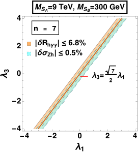
Figure 11: Contours by $\left|\delta\sigma_{Zh}\right|\leq 0.5\%$ (cyan band outlined with dashed lines) and $\left|\delta R_{h\gamma\gamma}\right|\leq 6.8\%$ (orange band outlined with solid lines) compared to the line (red solid) for $\lambda_{\text{eff}}=0$ for septuplet with fixed values of $M_{S_{A}}=9$ TeV and $M_{S_{B}}=300~{}\mathrm{GeV}$.

5 Conclusion

In this work we calculated the one-loop corrections on the Higgs-strahlung process $e^{+}e^{-}\to Zh$ in the presence of an extended scalar sector. In the case of zero or tiny VEV for the neutral scalar components, the BSM contribution may be computed separately from the SM EW corrections, making the calculation simpler than one might otherwise expect. We first classify the extended scalar sector according to their $\mathrm{SU\left(2\right)_{L}}$ representation. We then exhibit universal analytic expressions for the one-loop corrections in the $\overline{\mathrm{MS}}$ and on-shell schemes, and subsequently apply the results to representative scalar sector extensions.

Since the Higgs-strahlung process $e^{+}e^{-}\to Zh$ and the Higgs diphoton decay process $h\to\gamma\gamma$ are relatively sensitive to the BSM, we investigated the BSM contributions running in loops to these two independent processes to obtain the constraints on the scalar potentials in the extended scalar models. The projected precision at the CEPC for the inclusive $\sigma\left(Zh\right)$ and $h\to\gamma\gamma$ decay rate were assumed for purposes of concrete illustration. We note that the precision for the $Zh$ measurement with the Higgs decaying to bottom quark pair further reduces compared to the inclusive Higgs production. For instance, the estimated precision of $\sigma\left(Zh\right)\times\mathrm{BR}\left(h\to b\bar{b}\right)$ is 0.27% at the CEPC, which is approximately a half of the precision for the inclusive one. One might use narrow width approximation (NWA) to estimate the BSM contributions to the Higgs-strahlung process accompanying $h\to b\bar{b}$. Provided the extended scalar sector does not interact with the bottom quark, the BSM contributions to the full process in NWA would be simply broken down to the BSM loop effects to $\sigma\left(Zh\right)$ and BR$\left(h\to b\bar{b}\right)$ at LO. In this scenario the contour area of $\left|\delta\sigma_{Zh}\right|$ in the Fig. 3 - 11 constraining the parameter space in the extended scalar sector shrinks accordingly with higher precision whereas the complementarity or degeneracy between $Zh$ production and $h\to\gamma\gamma$ decay rate remains qualitatively. Nevertheless, due to the NWA accuracy Uhlemann:2008pm and the Yukawa coupling between the extended scalars and the bottom quark subject to $\mathcal{O}\left(\frac{m_{b}}{M_{W}}\right)$, the resulting uncertainty might offset the improvement of the precision by introducing the subsequent $h\to b\bar{b}$ channel.

Based on the numerical results, we found the following generic features in extended scalar models. First, similar to the oblique $T$ parameter, the $Zh$ cross section rate is sensitive to the mass splitting between different components of the multiplet. In the real triplet, quintuplet, and septuplet models there is no mass splitting at tree level . In these cases, $\sigma(Zh)$ and the $h\to\gamma\gamma$ signal rate are sensitive to similar regions of model parameter space. The situation differs for the complex triplet model, wherein the mass splitting arises at tree level and the two precision Higgs observables provide complementary parameter space probes . Second, if the mass spectrum in the multiplet has been identified at a hadron collider, one could further extract information on the new scalar-Higgs couplings from the precision Higgs observables analyzed here, because they depend on the new scalar masses, gauge couplings (fixed by gauge invariance), and extended scalar potential couplings. In principle, should the neutral component of the new scalar electroweak multiplet contribute to the dark matter relic density, these precision Higgs observables may further constrain the mass and interactions of some portion of the dark matter.

More specifically,

• In one class of models, such as the real scalar models, both the $e^{+}e^{-}\to Zh$ and diphoton processes probe similar parameter regions in the scalar potential. Thus, for example, should one observable yield a significant difference from SM expectations while the other fall in agreement with the SM, a particular model in this class may be disfavored.

• In another class of models, such as the complex triplet model, both the $e^{+}e^{-}\to Zh$ and $h\to\gamma\gamma$ processes probe complementary regions of parameter space. To again follow our example hypothetical experimental outcome, agreement with the SM in one observable, coupled with disagreement in the other measurement could be accommodated in this case.

One may also perform the foregoing analysis of $\sigma(Zh)$ and the $h\to\gamma\gamma$ signal rate for other versions of the two Higgs doublet model and singlet scalar models. In these extended scenarios, the new scalar may obtain a non-zero VEV, and thus the new scalar contribution cannot in general be extracted from the SM one. For $\sigma(Zh)$ in particular, one must calculate the full one-loop corrections, including both weak and QED corrections. Such a computation for $\sigma(Zh)$ in the Minimal Supersymmetric Standard Model Heinemeyer:2015qbu and Two Higgs Doublet Model Xie:2018yiv have recently appeared. The radiative corrections for $\sigma\left(Zh\right)$ in the Minimal Dilaton Model (MDM)  was considered in Cao:2014ita , where partial contributions were neglected due to their size in the MDM. Looking to the future, it would be interesting to compare the $Zh$ cross section in the other extended scalar models with and without vanishing VEVs.

Appendix A Feynman Rules

The Feynman rules with regard to the scalar multiplets coupling to gauge bosons are introduced via the kinetic term in the Lagrange $\mathcal{L}_{\mathrm{kin}}^{{\Phi}}\left(D_{\mu}{\Phi}\right)^{\dagger}\left(D^{\mu}{\Phi}\right)$ with the covariant derivative defined in Eq. (5), and the $\mathrm{SU\left(2\right)_{L}}$ generators $T^{a}$ in representation $j$ have the following generic matrix form,

$$T^{+}=\left(\begin{array}[]{ccccccc}0&\sqrt{2j}&0&0&\ldots&0&0\\ 0&0&\sqrt{2(2j-1)}&0&\ldots&0&0\\ 0&0&0&\sqrt{6(j-1)}&\ldots&0&0\\ \vdots&\vdots&\vdots&\vdots&\vdots&\vdots&\vdots\\ 0&0&0&0&\ldots&\sqrt{2(2j-1)}&0\\ 0&0&0&0&\ldots&0&\sqrt{2j}\\ 0&0&0&0&\ldots&0&0\end{array}\right),$$ (41)

$$T^{-}=\left(\begin{array}[]{ccccccc}0&0&0&\ldots&0&0&0\\ \sqrt{2j}&0&0&\ldots&0&0&0\\ 0&\sqrt{2(2j-1)}&0&\ldots&0&0&0\\ 0&0&\sqrt{6(j-1)}&\ldots&0&0&0\\ \vdots&\vdots&\vdots&\vdots&\vdots&\vdots&\vdots\\ 0&0&0&\ldots&\sqrt{2(2j-1)}&0&0\\ 0&0&0&\ldots&0&\sqrt{2j}&0\end{array}\right),$$ (49)

$$T^{3}=\left(\begin{array}[]{cccccc}j{}&~{}0{}&~{}0{}&~{}\ldots{}&~{}0{}&~{}0\\ 0{}&~{}j-1{}&~{}0{}&~{}\ldots{}&~{}0{}&~{}0\\ 0{}&~{}0{}&~{}j-2{}&~{}\ldots{}&~{}0{}&~{}0\\ \vdots{}&~{}\vdots{}&~{}\vdots{}&~{}\vdots{}&~{}\vdots{}&~{}\vdots\\ 0{}&~{}0{}&~{}0{}&~{}\ldots{}&~{}-j+1{}&~{}0\\ 0{}&~{}0{}&~{}0{}&~{}\ldots{}&~{}0{}&~{}-j\end{array}\right).$$ (56)

Expanding the kinetic Lagrange $\mathcal{L}_{\mathrm{kin}}^{{\Phi}}$ with the specific form of generator $T^{a}$ in representation $j$, it is easy to read off the trilinear and quartic couplings. The generic gauge Feynman rules are listed in Table. 3 below for the scalar multiplets,

Table 3: Gauge Feynman rules for the EW scalar multiplets

Vertices	Couplings
$S^{\mp Q}S^{\pm Q\mp 1}W_{\mu}^{\pm}$	$ig_{2}N_{S^{\mp}Q}N_{S^{\pm Q\mp 1}}\sqrt{2}\sqrt{\left(j+m\right)\left(j-m+1\right)}\left(k_{S^{\mp Q}}-k_{S^{\pm Q\mp 1}}\right)_{\mu}$, $(1\leq Q\leq j+\frac{Y}{2})$
$S^{Q}S^{-Q}W_{\mu}^{+}W_{\nu}^{-}$	$\pm 2g_{2}^{2}\left[j\left(j+1\right)-m^{2}\right]g_{\mu\nu}$
$S_{a}^{Q}S_{b}^{-Q}Z_{\mu}$	$\left(i\right)^{\delta_{ab}}\left(g_{2}c_{W}m+\left(-1\right)^{\delta_{ab}}g_{1}s_{W}\frac{Y}{2}\right)\left(k_{S^{Q}}-k_{S^{-Q}}\right)_{\mu}$
$S_{a}^{Q}S_{b}^{-Q}\gamma_{\mu}$	$\left(i\right)^{\delta_{ab}}\left(g_{2}s_{W}m-\left(-1\right)^{\delta_{ab}}g_{1}c_{W}\frac{Y}{2}\right)\left(k_{S^{Q}}-k_{S^{-Q}}\right)_{\mu}$
$S^{Q}S^{-Q}Z_{\mu}Z_{\nu}$	$2\left(g_{2}c_{W}m-g_{1}s_{W}\frac{Y}{2}\right)^{2}g_{\mu\nu}$
$S^{Q}S^{-Q}\gamma_{\mu}\gamma_{\nu}$	$2\left(g_{2}s_{W}m+g_{1}c_{W}\frac{Y}{2}\right)^{2}g_{\mu\nu}$
$S^{Q}S^{-Q}Z_{\mu}\gamma_{\nu}$	$2\left(g_{2}c_{W}m-g_{1}s_{W}\frac{Y}{2}\right)\left(g_{2}s_{W}m+g_{1}c_{W}\frac{Y}{2}\right)g_{\mu\nu}$

where the normalized factor $N_{S^{\mp}Q}N_{S^{\pm Q\mp 1}}=\left\langle{\Phi^{j\pm m}}\right|\left.{\Phi^{j\pm m\mp 1}}\right\rangle$, $Q=m+\frac{Y}{2}$ is the charge of the scalar component and positive definite in the first vertex that is indicated in parenthesis. The Feynman rules in the scalar potential are more complicated as they are representation dependent. In what follows, these Feynman rules are given in Table 4 for each model under consideration.

Table 4: Feynman rules in the scalar potential for Inert Doublet, Real/Complex Triplet, Quintuplet and Septuplet Models

Models	vertices	couplings
Inert Doublet: ${\Phi}=\begin{bmatrix}H^{+}\\ \frac{1}{\sqrt{2}}\left(H^{0}+iA^{0}\right)\end{bmatrix}$	$H^{+}H^{-}h$	$-\lambda_{3}v_{\phi}$
	$H^{0}H^{0}h$	$-\left(\lambda_{3}+\lambda_{4}+\lambda_{5}\right)v_{\phi}$
	$A^{0}A^{0}h$	$-\left(\lambda_{3}+\lambda_{4}-\lambda_{5}\right)v_{\phi}$
	$H^{+}H^{-}hh$	$-\lambda_{3}$
	$H^{0}H^{0}hh$	$-\left(\lambda_{3}+\lambda_{4}+\lambda_{5}\right)$
	$A^{0}A^{0}hh$	$-\left(\lambda_{3}+\lambda_{4}-\lambda_{5}\right)$
Real Triplet: ${\Phi}=\begin{bmatrix}H^{+},~{}H^{0},~{}-H^{-}\end{bmatrix}^{T}$	$H^{+}H^{-}h,~{}H^{0}H^{0}h$	$-\lambda_{3}v_{\phi}$
	$H^{+}H^{-}hh,~{}H^{0}H^{0}hh$	$-\lambda_{3}$
Complex Triplet: ${\Phi}=\begin{bmatrix}H^{++}\\ H^{+}\\ \frac{1}{\sqrt{2}}\left(H+iA\right)\end{bmatrix}$	$H^{++}H^{--}h$	$-\lambda_{4}v_{\phi}$
	$H^{+}H^{-}h$	$-\left(\lambda_{4}+\frac{\lambda_{5}}{2}\right)v_{\phi}$
	$HHh,~{}AAh$	$-\left(\lambda_{4}+\lambda_{5}\right)v_{\phi}$
	$H^{++}H^{--}hh$	$-\lambda_{4}$
	$H^{+}H^{-}hh$	$-\left(\lambda_{4}+\frac{\lambda_{5}}{2}\right)$
	$HHhh,~{}AAhh$	$-\left(\lambda_{4}+\lambda_{5}\right)$
Quintuplet ($n=5$) & Septuplet ($n=7$):  ${\Phi}=\begin{bmatrix}S_{A}^{j}+iS_{B}^{j}\\ iS_{A}^{j-1}-S_{B}^{j-1}\\ \vdots\\ S_{A}^{-j}+iS_{B}^{-j}\end{bmatrix}$	$S_{A}^{m}S_{A}^{-m}h,~{}\left(m=0,\ldots,j\right)$	$-\left(\lambda_{1}+\frac{2}{\sqrt{n}}\lambda_{3}\right)v_{\phi}$
	$S_{B}^{m}S_{B}^{-m}h,~{}\left(m=0,\ldots,j\right)$	$-\left(\lambda_{1}-\frac{2}{\sqrt{n}}\lambda_{3}\right)v_{\phi}$
	$S_{A}^{m}S_{A}^{-m}hh,~{}\left(m=0,\ldots,j\right)$	$-\left(\lambda_{1}+\frac{2}{\sqrt{n}}\lambda_{3}\right)$
	$S_{B}^{m}S_{B}^{-m}hh,~{}\left(m=0,\ldots,j\right)$	$-\left(\lambda_{1}-\frac{2}{\sqrt{n}}\lambda_{3}\right)$

Appendix B Potentials in Specific Models

Let us discuss the models with the extended scalar sector of dimension $n$. For the models under consideration in the context ($n=2,3,5,7$), there is an imposition of $\mathcal{Z}_{2}$ symmetry to have stable neutral component as DM candidate.

1. Real and Complex Singlet model Barger:2007im ; Barger:2008jx : In this case, usually $Y=0$ is taken, and thus additional term exists:

$$\left({\overline{H}}H\right)_{0}\Phi,\quad\left({\overline{\Phi}}\Phi\right)\Phi,\quad\Phi^{3}.$$ (57)

The scalar potential is

• real scalar singlet

  $$V\left(H,{\Phi}\right)= \frac{m^{2}}{2}{H}^{\dagger}{H}+\frac{\lambda}{4}\left({H}^{\dagger}{H}\right)^{2}+\frac{\delta_{1}}{2}{H}^{\dagger}{H}{\Phi}+\frac{\delta_{2}}{2}{H}^{\dagger}{H}{\Phi}^{2}$$ (58)

  $$+\left(\frac{\delta_{1}m^{2}}{2\lambda}\right){\Phi}+\frac{\kappa_{2}}{2}{\Phi}^{2}+\frac{\kappa_{3}}{3}{\Phi}^{3}+\frac{\kappa_{4}}{4}{\Phi}^{4}.$$

• complex scalar singlet

  $$V\left(H,{\Phi}\right)= \frac{m^{2}}{2}{H}^{\dagger}{H}+\frac{\lambda}{4}\left({H}^{\dagger}{H}\right)^{2}+\left(\frac{\left|\delta_{1}\right|e^{i\phi_{\delta_{1}}}}{4}{H}^{\dagger}{H}{\Phi}+\mathrm{h.c.}\right)+\frac{\delta_{2}}{2}{H}^{\dagger}{H}\left|{\Phi}\right|^{2}$$ (59)

  $$+\left(\frac{\left|\delta_{3}\right|e^{i\phi_{\delta_{3}}}}{4}{H}^{\dagger}{H}{\Phi}^{2}+\mathrm{h.c.}\right)+\left(\left|a_{1}\right|e^{i\phi_{a_{1}}}{\Phi}+\mathrm{h.c.}\right)+\left(\frac{\left|b_{1}\right|e^{i\phi_{b_{1}}}}{4}{\Phi}^{2}+\mathrm{h.c.}\right)$$

  $$+\frac{b_{2}}{2}\left|{\Phi}\right|^{2}+\left(\frac{\left|c_{1}\right|e^{i\phi_{c_{1}}}}{6}{\Phi}^{3}+\mathrm{h.c.}\right)+\left(\frac{\left|c_{2}\right|e^{i\phi_{c_{2}}}}{6}{\Phi}\left|{\Phi}\right|^{2}+\mathrm{h.c.}\right)$$

  $$+\left(\frac{\left|d_{1}\right|e^{i\phi_{d_{1}}}}{8}{\Phi}^{4}+\mathrm{h.c.}\right)+\left(\frac{\left|d_{3}\right|e^{i\phi_{d_{3}}}}{8}{\Phi}^{2}\left|{\Phi}\right|^{2}+\mathrm{h.c.}\right)+\frac{d_{2}}{4}\left|{\Phi}\right|^{4}$$

2. Two Higgs Doublet model Ma:2006km ; Barbieri:2006dq ; Branco:2011iw : For the complex doublet $n=2,Y=+1$, additional terms appear

$$\left[\left(HH\right)_{1}\left({\overline{\Phi}}~{}{\overline{\Phi}}\right)_{1}\right]_{0},\quad\left[\left(HH\right)_{1}\left({\overline{H}}~{}{\overline{\Phi}}\right)_{1}\right]_{0}\quad\left[\left(H\Phi\right)_{1}\left({\overline{\Phi}}~{}{\overline{\Phi}}\right)_{1}\right]_{0}.$$ (60)

If $n=2,Y=-1$, we have the above expression with $\Phi$ replaced by $\overline{\Phi}$. Thus the scalar potential in the two Higgs doublet model is written as

$$V\left({H},{\Phi}\right)= ~{}\mu_{1}^{2}~{}{H}^{\dagger}{H}+\mu_{2}^{2}~{}{\Phi}^{\dagger}{\Phi}+\mu_{12}^{2}\left({\Phi}^{\dagger}{H}+\mathrm{h.c.}\right)+\lambda_{1}\left({H}^{\dagger}{H}\right)^{2}+\lambda_{2}\left({\Phi}^{\dagger}{\Phi}\right)^{2}$$ (61)

$$+\lambda_{3}\left({H}^{\dagger}{H}\right)\left({\Phi}^{\dagger}{\Phi}\right)+\lambda_{4}\left({H}^{\dagger}{\Phi}\right)\left({\Phi}^{\dagger}{H}\right)+\left[\frac{\lambda_{5}}{2}\left({H}^{\dagger}{\Phi}\right)^{2}+\mathrm{h.c.}\right],$$

where the soft $\mathcal{Z}_{2}$ breaking term (the one $\propto\mu_{12}^{2}$) is dropped in the inert doublet model.

3. Real Triplet model Blank:1997qa ; FileviezPerez:2008bj ; Chen:2008jg : Here we consider $Y=0$. For real triplet $n=3,Y=0$, there are additional term

$$\left[\left({\overline{H}}H\right)_{1}\Phi\right]_{0}.$$ (62)

Thus the general potential is

$$V\left({H},{\Phi}\right)= ~{}\mu_{1}^{2}~{}{H}^{\dagger}{H}+\frac{\mu_{2}^{2}}{2}~{}{\Phi}^{\dagger}{\Phi}+\lambda_{1}\left({H}^{\dagger}{H}\right)^{2}+\frac{\lambda_{2}}{4}\left({\Phi}^{\dagger}{\Phi}\right)^{2}+\frac{\lambda_{3}}{2}\left({H}^{\dagger}{H}\right)\left({\Phi}^{\dagger}{\Phi}\right).$$ (63)

4. Complex Triplet model  AbdusSalam:2013eya ; Konetschny:1977bn ; Magg:1980ut ; Schechter:1980gr ; Cheng:1980qt : For the complex triplet, there is another possibility with $n=3,Y=\pm 2$, additional terms appear

$$\left[\left({\overline{H}}H\right)_{1}\overline{\Phi}\right]_{0},\quad\left[\left({\overline{H}}H\right)_{1}\Phi\right]_{0}.$$ (64)

The general potential is

$$V\left({H},{\Phi}\right)= ~{}\mu_{1}^{2}~{}{H}^{\dagger}{H}+\mu_{2}^{2}~{}{\Phi}^{\dagger}{\Phi}+\lambda_{1}\left({H}^{\dagger}{H}\right)^{2}+\lambda_{2}\left({\Phi}^{\dagger}{\Phi}\right)^{2}+\lambda_{3}\left|{\Phi}^{\dagger}T^{a}{\Phi}\right|^{2}$$ (65)

$$+\lambda_{4}{H}^{\dagger}{H}{\Phi}^{\dagger}{\Phi}+\lambda_{5}{H}^{\dagger}\tau^{a}{H}{\Phi}^{\dagger}T^{a}{\Phi}.$$

It is customary to write the complex scalar triplet fields in a $2\times 2$ representation $\Delta$. Following the notation of Du:2018eaw with $Y=2$, the potential is written

$$V\left({H},\Delta\right)= -m^{2}{H}^{\dagger}{H}+M^{2}\mathrm{Tr}\left(\Delta^{\dagger}\Delta\right)+\left(\mu{H}^{\mathrm{T}}i\tau_{2}\Delta^{\dagger}{H}+\mathrm{h.c.}\right)+\lambda_{1}\left({H}^{\dagger}{H}\right)^{2}+\lambda_{2}\mathrm{Tr}^{2}\left(\Delta^{\dagger}\Delta\right)$$ (66)

$$+\lambda_{3}\mathrm{Tr}\left(\Delta^{\dagger}\Delta\Delta^{\dagger}\Delta\right)+\lambda_{4}\left({H}^{\dagger}{H}\right)\mathrm{Tr}\left(\Delta^{\dagger}\Delta\right)+\lambda_{5}{H}^{\dagger}\Delta\Delta^{\dagger}{H},$$

with

$$\Delta=\left(\begin{array}[]{cc}\frac{\Delta^{+}}{\sqrt{2}}&H^{++}\\ \frac{1}{\sqrt{2}}\left(\delta+v_{\Delta}+i\eta\right)&-\frac{\Delta^{+}}{\sqrt{2}}\end{array}\right)$$

The relation between the $3\times 1$ and $2\times 2$ representation is

$$\Delta={\Phi}\cdot\tau^{a}.$$

5. Complex Quadruplet model AbdusSalam:2013eya : For complex triplet $n=4,Y=\pm 1$, additional terms appear

$$\left[\left(HH\right)_{1}\left({\overline{H}}~{}{\overline{\Phi}}\right)_{1}\right]_{0},\quad\left[\left(HH\right)_{1}\left({\overline{H}}{\Phi}\right)_{1}\right]_{0},$$ (67)

and for $Y=\pm 3$

$$\left[\left(HH\right)_{1}\left(H{\overline{\Phi}}\right)_{1}\right]_{0},\quad\left[\left(HH\right)_{1}\left(H{\Phi}\right)_{1}\right]_{0}.$$ (68)

The scalar potential is

$$V\left({H},{\Phi}\right)= ~{}\mu_{1}^{2}~{}{H}^{\dagger}{H}+\mu_{2}^{2}~{}{\Phi}^{\dagger}{\Phi}+\lambda_{1}\left({H}^{\dagger}{H}\right)^{2}+\lambda_{2}\left({\Phi}^{\dagger}{\Phi}\right)^{2}+\lambda_{3}\left|{\Phi}^{\dagger}T^{a}{\Phi}\right|^{2}$$ (69)

$$+\alpha{H}^{\dagger}{H}{\Phi}^{\dagger}{\Phi}+\beta{H}^{\dagger}\tau^{a}{H}{\Phi}^{\dagger}T^{a}{\Phi}+\gamma\left[\left({H}^{T}\epsilon\tau^{a}{H}\right)\left({\Phi}^{T}CT^{a}{\Phi}\right)^{\dagger}+\text{h.c.}\right],$$

where $C$ is an antisymmetric matrix defined as

$$CT^{a}C^{-1}=-T^{aT},$$

and its explicit form as well as that of $\epsilon$ can be found in appendix (6.2) in AbdusSalam:2013eya .

6. Complex and Real Quintuplet and Septuplet models Chao:2018xwz : For complex $n=5,7$ and $Y=0$, additional terms appear

$$\left[\left(\Phi{\Phi}\right)_{J}\Phi\right]_{0},\quad\left[\left(\Phi{\Phi}\right)_{J}{\overline{\Phi}}\right]_{0}.$$ (70)

The scalar potential is

$$V\left({H},{\Phi}\right)= ~{}-\mu^{2}~{}{H}^{\dagger}{H}+M_{A}^{2}\left({\Phi}^{\dagger}{\Phi}\right)+\left[M_{B}^{2}\left({\Phi}{\Phi}\right)_{0}+\mathrm{h.c.}\right]+\lambda\left({H}^{\dagger}{H}\right)^{2}$$ (71)

$$+\lambda_{1}\left({H}^{\dagger}{H}\right)\left({\Phi}^{\dagger}{\Phi}\right)+\lambda_{2}\left[\left(\overline{{H}}{H}\right)_{1}\left(\overline{{\Phi}}{\Phi}\right)_{1}\right]+\left[\lambda_{3}\left(\overline{{H}}{H}\right)_{0}\left(\overline{{\Phi}}{\Phi}\right)_{0}+\mathrm{h.c.}\right]$$

It was, however, noted that for the quintuplet ($n=5$) the stability of the DM is ensured by either the imposition of $\mathcal{Z}_{2}$ symmetry or a heavy mass scale $\Lambda$ well above the Planck scale inversely in a non-renormalizable dimension five operator; while for the septuplet ($n=7$) DM stability could be ensured by choosing $\Lambda$ below the Planck scale.

7. Generic models Chao:2018xwz : For generic multiplets other than special cases above, the general potential (except the mass terms) is written as

• Integer isospin $j$

  $$V\left({H},{\Phi}\right)= \sum_{J=0}^{2j}\lambda_{J}\left[\left({\Phi}{{\Phi}}\right)_{J}\left({\overline{\Phi}}\,{\overline{\Phi}}\right)_{J}\right]_{0}+\alpha\left({H}^{\dagger}{H}\right)\left({\Phi}^{\dagger}{\Phi}\right)+\beta\left[\left({\overline{H}}{H}\right)_{1}\left({\overline{\Phi}}{\Phi}\right)_{1}\right]_{0}$$ (72)

  $$+\delta_{0,Y}\Bigg{\{}\sum_{\kappa=0}^{2j}\left\{\lambda_{\kappa}^{\prime}\left[\left({\Phi}{\Phi}\right)_{\kappa}\left({\Phi}{\Phi}\right)_{\kappa}\right]_{0}+\lambda_{\kappa}^{\prime\prime}\left[\left(\overline{{\Phi}}{\Phi}\right)_{\kappa}\left({\Phi}{\Phi}\right)_{\kappa}\right]_{0}+\mathrm{h.c.}\right\}+\left[\gamma\left(\overline{{H}}{H}\right)_{0}\left({\Phi}{\Phi}\right)_{0}+\mathrm{h.c.}\right]$$

  $$+\delta_{0,j\left(\text{mod 2}\right)}\left[\mu_{1}\left({\Phi}\left({\Phi}{\Phi}\right)_{j}\right)_{0}+\mu_{2}\left(\overline{{\Phi}}\left({\Phi}{\Phi}\right)_{j}\right)_{0}+\text{h.c.}\right]\Bigg{\}}$$

• Half integer isospin $j$

  $$V\left({H},{\Phi}\right)= \sum_{J=1}^{2j}\lambda_{J}\left[\left({\Phi}{{\Phi}}\right)_{J}\left({\overline{\Phi}}\,{\overline{\Phi}}\right)_{J}\right]_{0}+\alpha\left({H}^{\dagger}{H}\right)\left({\Phi}^{\dagger}{\Phi}\right)+\beta\left[\left({\overline{H}}{H}\right)_{1}\left({\overline{\Phi}}{\Phi}\right)_{1}\right]_{0}$$ (73)

  $$+\delta_{0,Y}\Bigg{\{}\sum_{\kappa=1}^{2j}\left\{\lambda_{\kappa}^{\prime}\left[\left({\Phi}{\Phi}\right)_{\kappa}\left({\Phi}{\Phi}\right)_{\kappa}\right]_{0}+\lambda_{\kappa}^{\prime\prime}\left[\left(\overline{{\Phi}}{\Phi}\right)_{\kappa}\left({\Phi}{\Phi}\right)_{\kappa}\right]_{0}+\mathrm{h.c.}\right\}$$

  $$+\left\{\gamma\left[\left(\overline{{H}}{H}\right)_{1}\left({\Phi}{\Phi}\right)_{1}\right]_{0}+\mathrm{h.c.}\right\}\Bigg{\}}+\delta_{1,Y}\Bigg{\{}\Big{\{}\gamma_{1}\left[\left({H}{\Phi}\right)_{j+\frac{1}{2}}\left(\overline{{\Phi}}~{}\overline{{\Phi}}\right)_{j+\frac{1}{2}}\right]_{0}\delta_{0,j-\frac{1}{2}~{}\left(\text{mod 2}\right)}$$

  $$+\gamma_{2}\left[\left({H}{\Phi}\right)_{j-\frac{1}{2}}\left(\overline{{\Phi}}~{}\overline{{\Phi}}\right)_{j-\frac{1}{2}}\right]_{0}\delta_{0,j+\frac{1}{2}~{}\left(\text{mod 2}\right)}+\text{h.c.}\Big{\}}+\Big{\{}\kappa_{1}\left[\left({H}{H}\right)_{1}\left(\overline{{\Phi}}~{}\overline{{\Phi}}\right)_{1}\right]_{0}+\text{h.c.}\Big{\}}\Bigg{\}}$$

  $$+\delta_{-1,Y}\Bigg{\{}\Big{\{}\gamma_{1}\left[\left({H}\overline{{\Phi}}\right)_{j+\frac{1}{2}}\left({\Phi}{\Phi}\right)_{j+\frac{1}{2}}\right]_{0}\delta_{0,j-\frac{1}{2}~{}\left(\text{mod 2}\right)}+\gamma_{2}\left[\left({H}\overline{{\Phi}}\right)_{j-\frac{1}{2}}\left({\Phi}{\Phi}\right)_{j-\frac{1}{2}}\right]_{0}\delta_{0,j+\frac{1}{2}~{}\left(\text{mod 2}\right)}$$

  $$+\text{h.c.}\Big{\}}+\Big{\{}\kappa_{1}\left[\left({H}{H}\right)_{1}\left({\Phi}{\Phi}\right)_{1}\right]_{0}+\text{h.c.}\Big{\}}\Bigg{\}}$$

Appendix C Self Energy and Vertex Corrections

Since in the models under consideration the neutral components in the scalar multiplet sector decouple to that in the SM, one can treat the scalar multiplet loop contributions independently. The self energy and vertex loop contributions are written in terms of the one-, two- and three-point integrals. In the following the relevant scalar and vector/tensor integrals in D-dimension ($D=4-2\epsilon$), self energy and vertex corrections in each model are given, respectively.

C.1 The N-point Integrals with $N\leq 3$

The scalar one-point integral is

$$\frac{i}{16\pi^{2}}A_{0}\left(m\right)=\mu^{2\epsilon}\int\frac{d^{D}l}{\left(2\pi\right)^{D}}\frac{1}{l^{2}-m^{2}},$$ (74)

and $A_{0}\left(m\right)$ has simple form

$$A_{0}\left(m\right)=m^{2}\left(\frac{1}{\epsilon}+1+\log\frac{\mu^{2}}{m^{2}}\right)+\mathcal{O}\left(\epsilon\right).$$

The scalar and vector two-point integrals $B_{0,1}$ are defined as

$$\frac{i}{16\pi^{2}}\left(B_{0},B_{\mu}\right)\left(k,m_{1},m_{2}\right)=\mu^{2\epsilon}\int\frac{d^{D}l}{\left(2\pi\right)^{D}}\frac{\left(1,l_{\mu}\right)}{\left(l^{2}-m_{1}^{2}\right)\left[\left(l+k\right)^{2}-m_{2}^{2}\right]},$$ (75)

with $B_{\mu}=k_{\mu}B_{1}$ and

$$B_{0}\left(k,m_{1},m_{2}\right) =\frac{1}{\epsilon}-\int_{0}^{1}dx\log\frac{x^{2}k^{2}-x\left(k^{2}+m_{1}^{2}-m_{2}^{2}\right)+m_{1}^{2}-i\epsilon}{\mu^{2}}+\mathcal{O}\left(\epsilon\right),$$

$$B_{1}\left(k,m_{1},m_{2}\right) =\frac{1}{2k^{2}}\left[A_{0}\left(m_{1}\right)-A_{0}\left(m_{2}\right)-B_{0}\left(k,m_{1},m_{2}\right)\left(k^{2}+m_{1}^{2}-m_{2}^{2}\right)\right].$$

The scalar and (rank 2) tensor three-point integrals are

$$\frac{i}{16\pi^{2}}\left(C_{0},C_{\mu\nu}\right)\left(k_{1},k_{2},m_{1},m_{2},m_{3}\right)=\mu^{2\epsilon}\int\frac{d^{D}l}{\left(2\pi\right)^{D}}\frac{\left(1,l_{\mu}l_{\nu}\right)}{\left(l^{2}-m_{1}^{2}\right)\left[\left(l+k_{1}\right)^{2}-m_{2}^{2}\right]\left[\left(l+k_{1}+k_{2}\right)^{2}-m_{3}^{2}\right]},$$ (76)

with

$$C_{\mu\nu}=k_{1\mu}k_{1\nu}C_{21}+k_{2\mu}k_{2\nu}C_{22}+\left(k_{1\mu}k_{2\nu}+k_{2\mu}k_{1\nu}\right)C_{23}+g_{\mu\nu}C_{24},$$

where $C_{22},~{}C_{23},~{}C_{24}$ are the relevant contributions entering our calculation and their explicit expressions with specific arguments are given in C.3.

C.2 Gauge Boson Self energies

In the following the gauge boson self energies involving the virtual scalar multiplet contributions are given in the models below.

1. Inert Double

   $$\Sigma_{T}^{ZZ}\left(k^{2}\right) =\frac{1}{16\pi^{2}}\frac{1}{3}\times\Bigg{\{}+\frac{e^{2}\left(c_{W}^{2}-s_{W}^{2}\right)^{2}}{4c_{W}^{2}s_{W}^{2}}\left[4M_{H^{\pm}}^{2}B_{0}\left(0,M_{H^{\pm}},M_{H^{\pm}}\right)+\frac{2}{3}k^{2}+\left(k^{2}-4M_{H^{\pm}}^{2}\right)B_{0}\left(k,M_{H^{\pm}},M_{H^{\pm}}\right)\right]$$

   $$+\frac{e^{2}}{4c_{W}^{2}s_{W}^{2}}\bigg{[}-\frac{\left(M_{H^{0}}^{2}-M_{A^{0}}^{2}\right)^{2}}{k^{2}}-\frac{M_{H^{0}}^{2}-M_{A^{0}}^{2}}{k^{2}}\left[M_{H^{0}}^{2}B_{0}\left(0,M_{H^{0}},M_{H^{0}}\right)-M_{A^{0}}^{2}B_{0}\left(0,M_{A^{0}},M_{A^{0}}\right)\right]$$

   $$+2\left[M_{H^{0}}^{2}B_{0}\left(0,M_{H^{0}},M_{H^{0}}\right)+M_{A^{0}}^{2}B_{0}\left(0,M_{A^{0}},M_{A^{0}}\right)\right]+\frac{2}{3}k^{2}+\frac{\left(M_{H^{0}}^{2}-M_{A^{0}}^{2}\right)^{2}}{k^{2}}B_{0}\left(k,M_{H^{0}},M_{A^{0}}\right)$$

   $$+\left(k^{2}-2M_{H^{0}}^{2}-2M_{A^{0}}^{2}\right)B_{0}\left(k,M_{H^{0}},M_{A^{0}}\right)\bigg{]}\Bigg{\}}$$

   $$\Sigma_{T}^{\gamma Z}\left(k^{2}\right) =\frac{1}{16\pi^{2}}\frac{1}{3}\times\Bigg{\{}+\frac{e^{2}\left(c_{W}^{2}-s_{W}^{2}\right)}{2c_{W}s_{W}}\left[4M_{H^{\pm}}^{2}B_{0}\left(0,M_{H^{\pm}},M_{H^{\pm}}\right)+\frac{2}{3}k^{2}+\left(k^{2}-4M_{H^{\pm}}^{2}\right)B_{0}\left(k,M_{H^{\pm}},M_{H^{\pm}}\right)\right]\Bigg{\}}$$

   $$\Sigma_{T}^{\gamma\gamma}\left(k^{2}\right) =\frac{1}{16\pi^{2}}\frac{1}{3}\times\Bigg{\{}+e^{2}\left[4M_{H^{\pm}}^{2}B_{0}\left(0,M_{H^{\pm}},M_{H^{\pm}}\right)+\frac{2}{3}k^{2}+\left(k^{2}-4M_{H^{\pm}}^{2}\right)B_{0}\left(k,M_{H^{\pm}},M_{H^{\pm}}\right)\right]\Bigg{\}}$$

   $$\Sigma_{T}^{WW}\left(k^{2}\right) =\frac{1}{16\pi^{2}}\frac{1}{3}\times\frac{e^{2}}{4s_{W}^{2}}\Bigg{\{}-\frac{\left(M_{H^{\pm}}^{2}-M_{H^{0}}^{2}\right)^{2}}{k^{2}}B_{0}\left(0,M_{H^{\pm}},M_{H^{0}}\right)-\frac{\left(M_{H^{\pm}}^{2}-M_{A^{0}}^{2}\right)^{2}}{k^{2}}B_{0}\left(0,M_{H^{\pm}},M_{A^{0}}\right)$$

   $$+4M_{H^{\pm}}^{2}B_{0}\left(0,M_{H^{\pm}},M_{H^{\pm}}\right)+2M_{H^{0}}^{2}B_{0}\left(0,M_{H^{0}},M_{H^{0}}\right)+2M_{A^{0}}^{2}B_{0}\left(0,M_{A^{0}},M_{A^{0}}\right)+\frac{4}{3}k^{2}$$

   $$+\frac{1}{k^{2}}\left[\left(M_{H^{\pm}}-M_{H^{0}}\right)^{2}-k^{2}\right]\left[\left(M_{H^{\pm}}+M_{H^{0}}\right)^{2}-k^{2}\right]B_{0}\left(k,M_{H^{\pm}},M_{H^{0}}\right)$$

   $$+\frac{1}{k^{2}}\left[\left(M_{H^{\pm}}-M_{A^{0}}\right)^{2}-k^{2}\right]\left[\left(M_{H^{\pm}}+M_{A^{0}}\right)^{2}-k^{2}\right]B_{0}\left(k,M_{H^{\pm}},M_{A^{0}}\right)\Bigg{\}}$$

   $$\Sigma^{H}\left(k^{2}\right) =\frac{1}{16\pi^{2}}\times\Bigg{\{}+\lambda_{3}A_{0}\left(M_{H^{\pm}}\right)+\lambda_{3}^{2}v_{\phi}^{2}B_{0}\left(k,M_{H^{\pm}},M_{H^{\pm}}\right)$$

   $$+\frac{1}{2}\left[\lambda_{L}A_{0}\left(M_{H^{0}}\right)+\lambda_{L}^{2}v_{\phi}^{2}B_{0}\left(k,M_{H^{0}},M_{H^{0}}\right)+\lambda_{A}A_{0}\left(M_{A^{0}}\right)+\lambda_{A}^{2}v_{\phi}^{2}B_{0}\left(k,M_{A^{0}},M_{A^{0}}\right)\right]\Bigg{\}}$$ (77)

2. Real Triplet ($V_{1}V_{2}=ZZ,\gamma Z,WW,\gamma\gamma$)

   $$\Sigma_{T}^{V_{1}V_{2}}\left(k^{2}\right) =\frac{1}{16\pi^{2}}~{}\frac{1}{3}~{}g_{ssV_{1}}g_{ssV_{2}}\left[4M_{S}^{2}B_{0}\left(0,M_{S},M_{S}\right)+\frac{2}{3}k^{2}+\left(k^{2}-4M_{S}^{2}\right)B_{0}\left(k,M_{S},M_{S}\right)\right],$$ (78)

   $$\Sigma^{H}\left(k^{2}\right) =\frac{1}{16\pi^{2}}\frac{3}{2}\left[\lambda_{3}A_{0}\left(M_{S}\right)+\lambda_{3}^{2}v^{2}B_{0}\left(k,M_{S},M_{S}\right)\right].$$

3. Complex Triplet

   $$\begin{aligned} \Sigma_{T}^{ZZ}\left(k^{2}\right)&=\frac{1}{16\pi^{2}}\frac{1}{3}\times\Bigg{\{}+\frac{e^{2}s_{W}^{2}}{c_{W}^{2}}\left[4M_{H^{\pm}}^{2}B_{0}\left(0,M_{H^{\pm}},M_{H^{\pm}}\right)+\frac{2}{3}k^{2}+\left(k^{2}-4M_{H^{\pm}}^{2}\right)B_{0}\left(k,M_{H^{\pm}},M_{H^{\pm}}\right)\right]\\ &+\frac{e^{2}\left(c_{W}^{2}-s_{W}^{2}\right)^{2}}{c_{W}^{2}s_{W}^{2}}\left[4M_{H^{\pm\pm}}^{2}B_{0}\left(0,M_{H^{\pm\pm}},M_{H^{\pm\pm}}\right)+\frac{2}{3}k^{2}+\left(k^{2}-4M_{H^{\pm\pm}}^{2}\right)B_{0}\left(k,M_{H^{\pm\pm}},M_{H^{\pm\pm}}\right)\right]\\ &+\frac{e^{2}}{c_{W}^{2}s_{W}^{2}}\left[4M_{\Delta}^{2}B_{0}\left(0,M_{\Delta},M_{\Delta}\right)+\frac{2}{3}k^{2}+\left(k^{2}-4M_{\Delta}^{2}\right)B_{0}\left(k,M_{\Delta},M_{\Delta}\right)\right]\Bigg{\}}\end{aligned}$$ (79)

   $$\begin{aligned} \Sigma_{T}^{\gamma Z}\left(k^{2}\right)&=\frac{1}{16\pi^{2}}\frac{1}{3}\times\Bigg{\{}-\frac{e^{2}s_{W}}{c_{W}}\left[4M_{H^{\pm}}^{2}B_{0}\left(0,M_{H^{\pm}},M_{H^{\pm}}\right)+\frac{2}{3}k^{2}+\left(k^{2}-4M_{H^{\pm}}^{2}\right)B_{0}\left(k,M_{H^{\pm}},M_{H^{\pm}}\right)\right]\\ &+\frac{2e^{2}\left(c_{W}^{2}-s_{W}^{2}\right)}{c_{W}s_{W}}\left[4M_{H^{\pm\pm}}^{2}B_{0}\left(0,M_{H^{\pm\pm}},M_{H^{\pm\pm}}\right)+\frac{2}{3}k^{2}+\left(k^{2}-4M_{H^{\pm\pm}}^{2}\right)B_{0}\left(k,M_{H^{\pm\pm}},M_{H^{\pm\pm}}\right)\right]\Bigg{\}}\end{aligned}$$

   $$\begin{aligned} \Sigma_{T}^{\gamma\gamma}\left(k^{2}\right)&=\frac{1}{16\pi^{2}}\frac{1}{3}\times\Bigg{\{}+e^{2}\left[4M_{H^{\pm}}^{2}B_{0}\left(0,M_{H^{\pm}},M_{H^{\pm}}\right)+\frac{2}{3}k^{2}+\left(k^{2}-4M_{H^{\pm}}^{2}\right)B_{0}\left(k,M_{H^{\pm}},M_{H^{\pm}}\right)\right]\\ &+4e^{2}\left[4M_{H^{\pm\pm}}^{2}B_{0}\left(0,M_{H^{\pm\pm}},M_{H^{\pm\pm}}\right)+\frac{2}{3}k^{2}+\left(k^{2}-4M_{H^{\pm\pm}}^{2}\right)B_{0}\left(k,M_{H^{\pm\pm}},M_{H^{\pm\pm}}\right)\right]\Bigg{\}}\end{aligned}$$

   $$\begin{aligned} \Sigma_{T}^{WW}\left(k^{2}\right)&=\frac{1}{16\pi^{2}}\frac{1}{3}\times\frac{e^{2}}{s_{W}^{2}}\Bigg{\{}-\frac{\left(M_{H^{\pm}}^{2}-M_{\Delta}^{2}\right)^{2}}{k^{2}}B_{0}\left(0,M_{H^{\pm}},M_{\Delta}\right)-\frac{\left(M_{H^{\pm\pm}}^{2}-M_{H^{\pm}}^{2}\right)^{2}}{k^{2}}B_{0}\left(0,M_{H^{\pm\pm}},M_{H^{\pm}}\right)\\ &+2M_{\Delta}^{2}B_{0}\left(0,M_{\Delta},M_{\Delta}\right)+4M_{H^{\pm}}^{2}B_{0}\left(0,M_{H^{\pm}},M_{H^{\pm}}\right)+2M_{H^{\pm\pm}}^{2}B_{0}\left(0,M_{H^{\pm\pm}},M_{H^{\pm\pm}}\right)+\frac{4}{3}k^{2}\\ &+\frac{1}{k^{2}}\left[\left(M_{H^{\pm}}-M_{\Delta}\right)^{2}-k^{2}\right]\left[\left(M_{H^{\pm}}+M_{\Delta}\right)^{2}-k^{2}\right]B_{0}\left(k,M_{H^{\pm}},M_{\Delta}\right)\\ &+\frac{1}{k^{2}}\left[\left(M_{H^{\pm\pm}}-M_{H^{\pm}}\right)^{2}-k^{2}\right]\left[\left(M_{H^{\pm\pm}}+M_{H^{\pm}}\right)^{2}-k^{2}\right]B_{0}\left(k,M_{H^{\pm\pm}},M_{H^{\pm}}\right)\Bigg{\}}\end{aligned}$$

   $$\begin{aligned} \Sigma^{H}\left(k^{2}\right)&=\frac{1}{16\pi^{2}}\times\Bigg{\{}+\left(\lambda_{4}+\frac{\lambda_{5}}{2}\right)A_{0}\left(M_{H^{\pm}}\right)+\left(\lambda_{4}+\frac{\lambda_{5}}{2}\right)^{2}v_{\phi}^{2}B_{0}\left(k,M_{H^{\pm}},M_{H^{\pm}}\right)\\ &+\lambda_{4}A_{0}\left(M_{H^{\pm\pm}}\right)+\lambda_{4}^{2}v_{\phi}^{2}B_{0}\left(k,M_{H^{\pm\pm}},M_{H^{\pm\pm}}\right)\\ &+\left(\lambda_{4}+\lambda_{5}\right)A_{0}\left(M_{\Delta}\right)+\left(\lambda_{4}+\lambda_{5}\right)^{2}v_{\phi}^{2}B_{0}\left(k,M_{\Delta},M_{\Delta}\right)\Bigg{\}}\end{aligned}$$

4. Quintuplet ($n=5$) and Septuplet ($n=7$)

   $$\Sigma_{T}^{V_{1}V_{2}}\left(k^{2}\right)= \frac{1}{16\pi^{2}}\frac{1}{3}\times\Bigg{\{}\sum_{i=A}^{B}\left(\sum_{m=0}^{m=\frac{n-1}{2}}g_{S_{i}^{m}S_{i}^{-m+q}V_{1}}\cdot g_{S_{i}^{m}S_{i}^{-m+q}V_{2}}\right)\Big{[}4M_{S_{i}}^{2}B_{0}\left(0,M_{S_{i}},M_{S_{i}}\right)+\frac{2}{3}k^{2}$$

   $$+\left(k^{2}-4M_{S_{i}}^{2}\right)B_{0}\left(k,M_{S_{i}},M_{S_{i}}\right)\Big{]}\Bigg{\}},$$

   $$\left(q=1~{}\mathrm{for}~{}V_{1}V_{2}=WW,~{}q=0~{}\mathrm{for}~{}V_{1}V_{2}=ZZ,\gamma Z,\gamma\gamma\right)$$

   $$\Sigma^{h}\left(k^{2}\right)= \frac{1}{16\pi^{2}}\frac{n}{2}\sum_{i=A}^{B}\Bigg{[}-g_{S_{i}S_{i}hh}A_{0}\left(M_{S_{i}}\right)+g_{S_{i}S_{i}h}^{2}B_{0}\left(k,M_{S_{i}},M_{S_{i}}\right)\Bigg{]},$$

   $$\left(g_{S_{i}S_{i}h}=g_{S_{i}S_{i}hh}\cdot v,~{}g_{S_{A}S_{A}hh}=-\lambda_{1}-\frac{2}{\sqrt{n}}\lambda_{3},~{}g_{S_{B}S_{B}hh}=-\lambda_{1}+\frac{2}{\sqrt{n}}\lambda_{3}\right)$$ (80)

C.3 Three-point Tensor Integrals

The vertex contribution is given in Eq. (18). In addition to $B_{0}$ given in C.1, the explicit expressions of $C_{22s},~{}C_{23s},~{}C_{24s}$ are given below. The subscript ${}^{\prime}s^{\prime}$ and arguments $\left(M_{1},M_{2}\right)$ are short for the full arguments for the three-point functions that $C_{..s}\left(M_{1},M_{2}\right)=C_{..}\left(k_{1},k_{2},M_{1},M_{2},M_{2}\right)$, and $k_{1}^{2}=M_{Z}^{2},~{}k_{2}^{2}=M_{h}^{2},~{}\left(k_{1}+k_{2}\right)^{2}=s$. The masses $\left(M_{1},M_{2}\right)$ represent the masses of the scalar components in each model, where $M_{1}=M_{2}$ for each single vertex contribution except in the Inert Doublet when two neutral components as virtual particles in the loop and one should take $\left(M_{1},M_{2}\right)=\left(M_{H^{0}},M_{A^{0}}\right),~{}\left(M_{A^{0}},M_{H^{0}}\right)$ respectively for two types of vertex correction.

$$C_{22s}\left(M_{1},M_{2}\right) =\frac{1}{2\left[M_{h}^{4}+\left(M_{Z}^{2}-s\right)^{2}-2M_{h}^{2}\left(M_{Z}^{2}+s\right)\right]^{2}}\Bigg{\{}2M_{Z}^{2}\left[M_{h}^{4}+\left(M_{Z}^{2}-s\right)^{2}-2M_{h}^{2}\left(M_{Z}^{2}+s\right)\right]$$

$$-\frac{1}{s}\left(M_{h}^{2}-M_{Z}^{2}-s\right)\left[M_{h}^{4}+\left(M_{Z}^{2}-s\right)^{2}-2M_{h}^{2}\left(M_{Z}^{2}+s\right)\right]\left[A_{0}\left(M_{1}\right)-A_{0}\left(M_{2}\right)\right]$$

$$-6M_{Z}^{2}\left[M_{Z}^{2}\left(M_{h}^{2}-M_{Z}^{2}+s\right)+\left(M_{1}^{2}-M_{2}^{2}\right)\left(M_{h}^{2}+M_{Z}^{2}-s\right)\right]B_{0}\left(k_{1},M_{1},M_{2}\right)$$

$$-\bigg{[}M_{h}^{6}+\left(M_{Z}^{2}-s\right)^{2}\left(3M_{Z}^{2}-s\right)-M_{h}^{4}\left(5M_{Z}^{2}+3s\right)+M_{h}^{2}\left(M_{Z}^{4}+3s^{2}\right)$$

$$-2\left(M_{1}^{2}-M_{2}^{2}\right)\left(M_{h}^{4}+M_{h}^{2}\left(4M_{Z}^{2}-s\right)+\left(M_{Z}^{2}-s\right)^{2}\right)\bigg{]}B_{0}\left(k_{2},M_{2},M_{2}\right)$$

$$+\bigg{[}\left(M_{h}^{2}-3M_{Z}^{2}\right)\left(M_{h}^{2}-M_{Z}^{2}\right)^{2}-\left(3M_{h}^{4}+M_{Z}^{4}\right)s+\left(3M_{h}^{2}+5M_{Z}^{2}\right)s^{2}-s^{3}$$

$$+\frac{1}{s}\left(M_{1}^{2}-M_{2}^{2}\right)\left(\left(M_{h}^{2}-M_{Z}^{2}\right)^{3}-5\left(M_{h}^{4}-M_{Z}^{4}\right)s+\left(7M_{h}^{2}-M_{Z}^{2}\right)s^{2}-3s^{3}\right)\bigg{]}B_{0}\left(k_{1}+k_{2},M_{1},M_{2}\right)$$

$$+2\bigg{[}M_{Z}^{4}\left(M_{h}^{4}-2M_{h}^{2}\left(M_{Z}^{2}-2s\right)+\left(M_{Z}^{2}-s\right)\right)+\left(M_{1}^{4}+M_{2}^{4}\right)\left(M_{h}^{4}+2M_{h}^{2}\left(2M_{Z}^{2}-s\right)+\left(M_{Z}^{2}-s\right)^{2}\right)$$

$$-2M_{Z}^{2}\left(M_{h}^{4}\left(-2M_{1}^{2}+M_{2}^{2}\right)+\left(M_{Z}^{2}-s\right)^{2}\left(M_{1}^{2}-2M_{2}^{2}\right)+M_{h}^{2}\left(M_{Z}^{2}+s\right)\left(M_{1}^{2}+M_{2}^{2}\right)\right)$$

$$-2M_{1}^{2}M_{2}^{2}\left[M_{h}^{4}+2M_{h}^{2}\left(2M_{Z}^{2}-s\right)+\left(M_{Z}^{2}-s\right)^{2}\right]\bigg{]}C_{0}\left(k_{1},k_{2},M_{1},M_{2},M_{2}\right)\Bigg{\}}$$

$$C_{23s}\left(M_{1},M_{2}\right) =\frac{1}{2\left[M_{h}^{4}+\left(M_{Z}^{2}-s\right)^{2}-2M_{h}^{2}\left(M_{Z}^{2}+s\right)\right]^{2}}\Bigg{\{}\left(M_{h}^{2}+M_{Z}^{2}-s\right)\left[M_{h}^{4}+\left(M_{Z}^{2}-s\right)^{2}-2M_{h}^{2}\left(M_{Z}^{2}+s\right)\right]$$

$$-\frac{1}{s}\left(M_{h}^{2}-M_{Z}^{2}+s\right)\left(M_{h}^{4}+\left(M_{Z}^{2}-s\right)^{2}-2M_{h}^{2}\left(M_{Z}^{2}+s\right)\right)\left[A_{0}\left(M_{1}\right)-A_{0}\left(M_{2}\right)\right]$$

$$+\bigg{[}M_{Z}^{2}\left(-M_{h}^{4}+5\left(M_{Z}^{2}-s\right)^{2}-4M_{h}^{2}\left(M_{Z}^{2}+s\right)\right)$$

$$-\left(M_{1}^{2}-M_{2}^{2}\right)\left(M_{h}^{4}+\left(M_{Z}^{2}-s\right)^{2}+2M_{h}^{2}\left(5M_{Z}^{2}-s\right)\right)\bigg{]}B_{0}\left(k_{1},M_{1},M_{2}\right)$$

$$-\bigg{[}M_{h}^{6}+2\left(M_{Z}^{2}-s\right)^{3}-2M_{h}^{4}\left(3M_{Z}^{2}+2s\right)+M_{h}^{2}\left(3M_{Z}^{4}-8M_{Z}^{2}s+5s^{2}\right)$$

$$-6\left(M_{1}^{2}-M_{2}^{2}\right)M_{h}^{2}\left(M_{h}^{2}+M_{Z}^{2}-s\right)\bigg{]}B_{0}\left(k_{2},M_{2},M_{2}\right)$$

$$+\bigg{[}M_{h}^{6}-\left(M_{Z}^{2}-s\right)^{2}\left(3M_{Z}^{2}+2s\right)-M_{h}^{4}\left(5M_{Z}^{2}+4s\right)+M_{h}^{2}\left(7M_{Z}^{4}-4M_{Z}^{2}s+5s^{2}\right)$$

$$+\left(M_{1}^{2}-M_{2}^{2}\right)\left(\left(M_{h}^{2}-M_{Z}^{2}\right)^{2}+2\left(-3M_{h}^{4}+M_{h}^{2}M_{Z}^{2}+2M_{Z}^{4}\right)s+\left(3M_{h}^{2}-5M_{Z}^{2}\right)s^{2}+2s^{3}\right)\bigg{]}B_{0}\left(k_{1}+k_{2},M_{1},M_{2}\right)$$

$$+2\bigg{[}M_{Z}^{2}\left(\left(M_{Z}^{2}-s\right)^{3}+M_{h}^{4}\left(M_{Z}^{2}+2s\right)-M_{h}^{2}\left(2M_{Z}^{4}-3M_{Z}^{2}s+2s^{2}\right)\right)$$

$$+3\left(M_{1}^{4}+M_{2}^{4}\right)M_{h}^{2}\left(M_{h}^{2}+M_{Z}^{2}-s\right)+M_{1}^{2}\left(M_{h}^{2}-M_{Z}^{2}+s\right)\left(M_{h}^{4}+2M_{h}^{2}\left(2M_{Z}^{2}-s\right)+\left(M_{Z}^{2}-s\right)^{2}\right)$$

$$+2M_{2}^{2}\left(\left(M_{Z}^{2}-s\right)^{3}-M_{h}^{4}\left(2M_{Z}^{2}+s\right)+M_{h}^{2}\left(M_{Z}^{4}-3M_{Z}^{2}s+2s^{2}\right)\right)$$

$$-6M_{1}^{2}M_{2}^{2}M_{h}^{2}\left(M_{h}^{2}+M_{Z}^{2}-s\right)\bigg{]}C_{0}\left(k_{1},k_{2},M_{1},M_{2},M_{2}\right)\Bigg{\}}$$

$$C_{24s}\left(M_{1},M_{2}\right) =\frac{1}{4\left[M_{h}^{4}+\left(M_{Z}^{2}-s\right)^{2}-2M_{h}^{2}\left(M_{Z}^{2}+s\right)\right]}\Bigg{\{}M_{h}^{4}+\left(M_{Z}^{2}-s\right)^{2}-2M_{h}^{2}\left(M_{Z}^{2}+s\right)$$

$$-\left[M_{Z}^{2}\left(M_{h}^{2}-M_{Z}^{2}+s\right)+\left(M_{1}^{2}-M_{2}^{2}\right)\left(M_{h}^{2}+M_{Z}^{2}-s\right)\right]B_{0}\left(k_{1},M_{1},M_{2}\right)$$

$$+M_{h}^{2}\left(M_{h}^{2}-M_{Z}^{2}-s+2M_{1}^{2}-2M_{2}^{2}\right)B_{0}\left(k_{2},M_{2},M_{2}\right)$$

$$+\left[s\left(-Mh^{2}-Mz^{2}+s\right)-\left(M_{1}^{2}-M_{2}^{2}\right)\left(M_{h}^{2}-M_{Z}^{2}+s\right)\right]B_{0}\left(k_{1}+k_{2},M_{1},M_{2}\right)$$

$$+2\bigg{[}M_{h}^{2}M_{Z}^{2}s+\left(M_{1}^{4}+M_{2}^{4}\right)M_{h}^{2}+M_{1}^{2}M_{h}^{2}\left(M_{h}^{2}-M_{Z}^{2}-s\right)+M_{2}^{2}\left(\left(M_{Z}^{2}-s\right)^{2}-M_{h}^{2}\left(M_{Z}^{2}+s\right)\right)$$

$$-2M_{1}^{2}M_{2}^{2}M_{h}^{2}\bigg{]}C_{0}\left(k_{1},k_{1},M_{1},M_{2},M_{2}\right)\Bigg{\}}$$ (81)

Appendix D On-shell Renormalization Scheme

The on-shell (OS) renormalization conditions consist of two parts: (a) the pole of the propagator defines the real part of the renormalized mass; (b) the real part of the residue of the propagator is equal to one. The renormalized quantities and renormalization constants are in accordance with the scheme of Denner Denner:1991kt , and are defined as follows

$$M_{W,0}^{2} =M_{W}^{2}+\delta M_{W}^{2},$$ (82)

$$M_{Z,0}^{2} =M_{Z}^{2}+\delta M_{Z}^{2},$$

$$M_{h,0}^{2} =M_{h}^{2}+\delta M_{h}^{2},$$

$$W_{0}^{\pm} =Z_{W}^{1/2}W^{\pm}=\left(1+\frac{1}{2}\delta Z_{W}\right)W^{\pm},$$

$$\begin{pmatrix}Z_{0}\\ A_{0}\end{pmatrix} =\begin{pmatrix}Z_{ZZ}^{1/2}&Z_{Z\gamma}^{1/2}\\ Z_{\gamma Z}^{1/2}&Z_{\gamma\gamma}\end{pmatrix}\begin{pmatrix}Z\\ A\end{pmatrix}=\begin{pmatrix}1+\frac{1}{2}\delta Z_{ZZ}&\frac{1}{2}\delta Z_{Z\gamma}\\ \frac{1}{2}\delta Z_{\gamma Z}&1+\frac{1}{2}\delta Z_{\gamma\gamma}\end{pmatrix}\begin{pmatrix}Z\\ A\end{pmatrix}$$

$$h_{0} =Z_{h}^{1/2}h=\left(1+\frac{1}{2}\delta Z_{h}\right)h,$$

where quantities with subscript $0$ denote the bare parameters.

In terms of the renormalized self-energy functions which are denoted with caret (one should differentiate this with the caret notation in $\overline{\mathrm{MS}}$ scheme), the OS conditions are given

$$\mathrm{Re}~{}\hat{\Sigma}_{T}^{WW}\left(M_{W}^{2}\right)=\delta M_{W}^{2},\quad\mathrm{Re}\left.\frac{\partial\hat{\Sigma}_{T}^{WW}\left(k^{2}\right)}{\partial k^{2}}\right|_{k^{2}=M_{W}^{2}}=0,$$ (83)

$$\mathrm{Re}~{}\hat{\Sigma}_{T}^{ZZ}\left(M_{Z}^{2}\right)=\delta M_{Z}^{2},\quad\mathrm{Re}\left.\frac{\partial\hat{\Sigma}_{T}^{ZZ}\left(k^{2}\right)}{\partial k^{2}}\right|_{k^{2}=M_{Z}^{2}}=0,$$

$$\hat{\Sigma}_{T}^{\gamma\gamma}\left(0\right)=0,\quad\mathrm{Re}\left.\frac{\partial\hat{\Sigma}_{T}^{\gamma\gamma}\left(k^{2}\right)}{\partial k^{2}}\right|_{k^{2}=0}=0,$$

$$\mathrm{Re}~{}\hat{\Sigma}_{T}^{\gamma Z}\left(M_{Z}^{2}\right)=\hat{\Sigma}_{T}^{\gamma Z}\left(0\right)=0,$$

$$\mathrm{Re}~{}\hat{\Sigma}^{h}\left(M_{h}^{2}\right)=\delta M_{h}^{2},\quad\mathrm{Re}\left.\frac{\partial\hat{\Sigma}^{h}\left(k^{2}\right)}{\partial k^{2}}\right|_{k^{2}=M_{h}^{2}}=0.$$

The mass and wave function renormalization counterterms are then determined by the following relations

$$\delta M_{W}^{2}=\mathrm{Re}~{}\Sigma_{T}^{WW}\left(M_{W}^{2}\right),\quad\delta Z_{W}=-\mathrm{Re}\left.\frac{\partial\Sigma_{T}^{WW}\left(k^{2}\right)}{\partial k^{2}}\right|_{k^{2}=M_{W}^{2}},$$ (84)

$$\delta M_{Z}^{2}=\mathrm{Re}~{}\Sigma_{T}^{ZZ}\left(M_{Z}^{2}\right),\quad\delta Z_{ZZ}=-\mathrm{Re}\left.\frac{\partial\Sigma_{T}^{ZZ}\left(k^{2}\right)}{\partial k^{2}}\right|_{k^{2}=M_{Z}^{2}},$$

$$\delta Z_{\gamma\gamma}=-\mathrm{Re}\left.\frac{\partial\Sigma_{T}^{\gamma\gamma}\left(k^{2}\right)}{\partial k^{2}}\right|_{k^{2}=0},$$

$$\delta Z_{\gamma Z}=-2~{}\mathrm{Re}~{}\frac{\Sigma_{T}^{\gamma Z}\left(M_{Z}^{2}\right)}{M_{Z}^{2}},\quad\delta Z_{Z\gamma}=2\frac{\Sigma_{T}^{\gamma Z}\left(0\right)}{M_{Z}^{2}},$$

$$\delta M_{h}^{2}=\mathrm{Re}~{}\Sigma^{h}\left(M_{h}^{2}\right),\quad\delta Z_{h}=-\mathrm{Re}\left.\frac{\partial\Sigma^{h}\left(k^{2}\right)}{\partial k^{2}}\right|_{k^{2}=M_{h}^{2}},$$

where the expressions of the unrenormalized self energies for each scalar multiplet model can be found in Appendix C.2.

The counter terms of self-energy that are relevant to our calculation read

$$\includegraphics[scale={0.6},valign={c}]{figure/self_ct}=\left\{\begin{tabular}[]{l}$-i~{}\delta\Sigma_{T}^{WW}=-i\left[\left(k^{2}-M_{W}^{2}\right)\delta Z_{W}-\delta M_{W}^{2}\right]$,\\ $-i~{}\delta\Sigma_{T}^{ZZ}=-i\left[\left(k^{2}-M_{Z}^{2}\right)\delta Z_{ZZ}-\delta M_{Z}^{2}\right]$,\\ $-i~{}\delta\Sigma_{T}^{\gamma Z}=-\frac{i}{2}\left[\left(k^{2}-M_{Z}^{2}\right)\delta Z_{Z\gamma}+k^{2}\delta Z_{\gamma Z}\right]$,\end{tabular}\right.$$ (85)

so that one can obtain the renormalized self-energies according to

$$\hat{\Sigma}_{T}^{V_{1}V_{2}}\left(k^{2}\right)=\Sigma_{T}^{V_{1}V_{2}}\left(k^{2}\right)+\delta\Sigma_{T}^{V_{1}V_{2}}.$$

The self-energy contributions in terms of matrix element square factorize to Born, which read

$$2~{}\mathrm{Re}\left[\left(\delta{\bf M}_{\mathrm{self}}^{ZZ}+\delta{\bf M}_{\mathrm{self}}^{\gamma Z}\right)\cdot{\bf M}_{LO}^{*}\right]$$ (86)

$$= 2\frac{2e^{4}}{s_{W}^{2}c_{W}^{2}}\left[-\frac{\left(g_{v}^{2}+g_{a}^{2}\right)\left(s-M_{Z}^{2}\right)}{\left(s-M_{Z}^{2}\right)^{2}+M_{Z}^{2}\Gamma_{Z}^{2}}\cdot\hat{\Sigma}_{T}^{ZZ}\left(s\right)-\frac{g_{v}}{s}\cdot\hat{\Sigma}_{T}^{\gamma Z}\left(s\right)\right]\frac{tu+2sM_{Z}^{2}-M_{h}^{2}M_{Z}^{2}}{\left(s-M_{Z}^{2}\right)^{2}+M_{Z}^{2}\Gamma_{Z}^{2}}$$

It should be noted that the vertex contribution per se is UV finite. Using OS renormalization scheme, one has to cross check if the corresponding counter term contribution is also UV finite. The vertex counter terms have the following contributions,

$$\includegraphics[scale={0.6},valign={c}]{figure/vert_ct}=\left\{\begin{tabular}[]{ll}$ieg_{\mu\nu}\cdot\delta_{\mathrm{ct}}^{ZZh}$:&$\delta Z_{e}+\frac{2s_{W}^{2}-c_{W}^{2}}{c_{W}^{2}}\frac{\delta s_{W}}{s_{W}}+\frac{1}{2}\frac{\delta M_{W}^{2}}{M_{W}^{2}}+\frac{1}{2}\delta Z_{h}+\delta Z_{ZZ}$\\ $ieg_{\mu\nu}\cdot\delta_{\mathrm{ct}}^{\gamma Zh}$:&$\frac{1}{2}\delta Z_{Z\gamma}$\end{tabular}\right.$$ (87)

where $\delta Z_{e}$ and $\delta s_{W}^{2}/s_{W}^{2}$ can be written in terms of the mass and field renormalization constants (FRCs) that

$$\delta Z_{e}=-\frac{1}{2}\left(\delta Z_{\gamma\gamma}+\frac{s_{W}}{c_{W}}\delta Z_{Z\gamma}\right),\quad\frac{\delta s_{W}}{s_{W}}=-\frac{1}{2}\frac{c_{W}^{2}}{s_{W}^{2}}\left(\frac{\delta M_{W}^{2}}{M_{W}^{2}}-\frac{\delta M_{Z}^{2}}{M_{Z}^{2}}\right).$$ (88)

It is clear that both vertex counter terms in Eq.(87) are UV finite.

In addition to the final vertex ($(Z/\gamma)Zh$) counter term, one has to take the initial vertex ($e^{-}e^{+}Z$) counter term into account, even though there is no scalar loop corrections to the initial vertex. The counter term of the initial vertex $e^{-}e^{+}Z$ has the following form.

$$\includegraphics[scale={0.6},valign={c}]{figure/init_ct}=ie\gamma_{\mu}\left(\delta c_{v}-\delta c_{a}\gamma^{5}\right)$$ (89)

$$\delta c_{v}=\delta g_{v}+\frac{g_{v}}{2}\delta Z_{ZZ}-\frac{Q_{e}}{2}\delta Z_{\gamma Z},$$

$$\delta c_{a}=\delta g_{a}+\frac{g_{a}}{2}\delta Z_{ZZ},$$

where the variations of $\left(g_{v},~{}g_{a}\right)$ read

$$\delta g_{v}=\frac{I_{W,e}^{3}}{2s_{W}c_{W}}\left(\delta Z_{e}+\frac{s_{W}^{2}-c_{W}^{2}}{c_{W}^{2}}\frac{\delta s_{W}}{s_{W}}\right)-\frac{s_{W}}{c_{W}}Q_{e}\left(\delta Z_{e}+\frac{1}{c_{W}^{2}}\frac{\delta s_{W}}{s_{W}}\right),$$

$$\delta g_{a}=\frac{I_{W,e}^{3}}{2s_{W}c_{W}}\left(\delta Z_{e}+\frac{s_{W}^{2}-c_{W}^{2}}{c_{W}^{2}}\frac{\delta s_{W}}{s_{W}}\right),$$

with the quantum numbers for electron taking $I_{W,e}^{3}=-1/2,~{}Q_{e}=-1$. It is worth noting that the initial vertex counter term contribution is as well UV finite.

The vertex counter term stand alone contributions in terms of matrix element square take the form below,

$$2~{}\mathrm{Re}\left[\left(\delta{\bf M}_{\mathrm{vert,ct}}^{ZZh}+\delta{\bf M}_{\mathrm{vert,ct}}^{\gamma Zh}+\delta{\bf M}_{\mathrm{vert,ct}}^{e^{-}e^{+}Z}\right){\bf M}_{LO}^{*}\right]$$ (90)

$$= 2\frac{2e^{4}}{s_{W}^{2}c_{W}^{2}}\left(tu+2sM_{Z}^{2}-M_{h}^{2}M_{Z}^{2}\right)\times$$

$$\left\{\frac{\left(g_{v}^{2}+g_{a}^{2}\right)\delta_{\mathrm{ct}}^{ZZh}}{\left(s-M_{Z}^{2}\right)^{2}+M_{Z}^{2}\Gamma_{Z}^{2}}+\frac{g_{v}\left(s-M_{Z}^{2}\right)\delta_{\mathrm{ct}}^{\gamma Zh}}{s\left[\left(s-M_{Z}^{2}\right)^{2}+M_{Z}^{2}\Gamma_{Z}^{2}\right]}+\frac{\delta c_{v}g_{v}+\delta c_{a}g_{a}}{\left(s-M_{Z}^{2}\right)^{2}+M_{Z}^{2}\Gamma_{Z}^{2}}\right\}.$$

References

- (1) ATLAS Collaboration, Combined measurements of Higgs boson production and decay using up to fb-1 of proton–proton collision data at 13 TeV collected with the ATLAS experiment, .
- (2) CMS Collaboration, A. M. Sirunyan et. al., Combined measurements of Higgs boson couplings in proton–proton collisions at , Eur. Phys. J. C 79 (2019), no. 5 421 [1809.10733].
- (3) M. Cepeda et. al., Report from Working Group 2: Higgs Physics at the HL-LHC and HE-LHC, CERN Yellow Rep. Monogr. 7 (2019) 221–584 [1902.00134].
- (4) J. de Blas et. al., Higgs Boson Studies at Future Particle Colliders, JHEP 01 (2020) 139 [1905.03764].
- (5) FCC Collaboration, A. Abada et. al., FCC Physics Opportunities: Future Circular Collider Conceptual Design Report Volume 1, Eur. Phys. J. C 79 (2019), no. 6 474.
- (6) CEPC Study Group Collaboration, M. Dong et. al., CEPC Conceptual Design Report: Volume 2 - Physics & Detector, 1811.10545.
- (7) FCC Collaboration, A. Abada et. al., FCC-ee: The Lepton Collider: Future Circular Collider Conceptual Design Report Volume 2, Eur. Phys. J. ST 228 (2019), no. 2 261–623.
- (8) T. Barklow, J. Brau, K. Fujii, J. Gao, J. List, N. Walker and K. Yokoya, ILC Operating Scenarios, 1506.07830.
- (9) K. Fujii et. al., Physics Case for the 250 GeV Stage of the International Linear Collider, 1710.07621.
- (10) LCC Physics Working Group Collaboration, K. Fujii et. al., Tests of the Standard Model at the International Linear Collider, 1908.11299.
- (11) Projections for measurements of Higgs boson signal strengths and coupling parameters with the ATLAS detector at a HL-LHC, .
- (12) CMS Collaboration, Projected Performance of an Upgraded CMS Detector at the LHC and HL-LHC: Contribution to the Snowmass Process, in Community Summer Study 2013: Snowmass on the Mississippi, 7, 2013. 1307.7135.
- (13) S. Profumo, M. J. Ramsey-Musolf and G. Shaughnessy, Singlet Higgs phenomenology and the electroweak phase transition, JHEP 08 (2007) 010 [0705.2425].
- (14) J. R. Espinosa, T. Konstandin and F. Riva, Strong Electroweak Phase Transitions in the Standard Model with a Singlet, Nucl. Phys. B 854 (2012) 592–630 [1107.5441].
- (15) L. Niemi, H. H. Patel, M. J. Ramsey-Musolf, T. V. Tenkanen and D. J. Weir, Electroweak phase transition in the real triplet extension of the SM: Dimensional reduction, Phys. Rev. D 100 (2019), no. 3 035002 [1802.10500].
- (16) L. Niemi, M. J. Ramsey-Musolf, T. V. I. Tenkanen and D. J. Weir, Thermodynamics of a Two-Step Electroweak Phase Transition, Phys. Rev. Lett. 126 (2021), no. 17 171802 [2005.11332].
- (17) V. Barger, P. Langacker, M. McCaskey, M. J. Ramsey-Musolf and G. Shaughnessy, LHC Phenomenology of an Extended Standard Model with a Real Scalar Singlet, Phys. Rev. D 77 (2008) 035005 [0706.4311].
- (18) V. Barger, P. Langacker, M. McCaskey, M. Ramsey-Musolf and G. Shaughnessy, Complex Singlet Extension of the Standard Model, Phys. Rev. D 79 (2009) 015018 [0811.0393].
- (19) A. Papaefstathiou and G. White, The Electro-Weak Phase Transition at Colliders: Confronting Theoretical Uncertainties and Complementary Channels, 2010.00597.
- (20) M. Cirelli, N. Fornengo and A. Strumia, Minimal dark matter, Nucl. Phys. B 753 (2006) 178–194 [hep-ph/0512090].
- (21) J. McDonald, Gauge singlet scalars as cold dark matter, Phys. Rev. D 50 (1994) 3637–3649 [hep-ph/0702143].
- (22) C. Burgess, M. Pospelov and T. ter Veldhuis, The Minimal model of nonbaryonic dark matter: A Singlet scalar, Nucl. Phys. B 619 (2001) 709–728 [hep-ph/0011335].
- (23) M. A. Díaz, B. Koch and S. Urrutia-Quiroga, Constraints to Dark Matter from Inert Higgs Doublet Model, Adv. High Energy Phys. 2016 (2016) 8278375 [1511.04429].
- (24) E. Ma, Verifiable radiative seesaw mechanism of neutrino mass and dark matter, Phys. Rev. D 73 (2006) 077301 [hep-ph/0601225].
- (25) R. Barbieri, L. J. Hall and V. S. Rychkov, Improved naturalness with a heavy Higgs: An Alternative road to LHC physics, Phys. Rev. D 74 (2006) 015007 [hep-ph/0603188].
- (26) S. Banerjee and N. Chakrabarty, A revisit to scalar dark matter with radiative corrections, JHEP 05 (2019) 150 [1612.01973].
- (27) P. Fileviez Perez, H. H. Patel, M. Ramsey-Musolf and K. Wang, Triplet Scalars and Dark Matter at the LHC, Phys. Rev. D 79 (2009) 055024 [0811.3957].
- (28) T. Araki, C. Geng and K. I. Nagao, Dark Matter in Inert Triplet Models, Phys. Rev. D 83 (2011) 075014 [1102.4906].
- (29) T. Hambye, F.-S. Ling, L. Lopez Honorez and J. Rocher, Scalar Multiplet Dark Matter, JHEP 07 (2009) 090 [0903.4010]. [Erratum: JHEP 05, 066 (2010)].
- (30) S. S. AbdusSalam and T. A. Chowdhury, Scalar Representations in the Light of Electroweak Phase Transition and Cold Dark Matter Phenomenology, JCAP 05 (2014) 026 [1310.8152].
- (31) W. Chao, G.-J. Ding, X.-G. He and M. Ramsey-Musolf, Scalar Electroweak Multiplet Dark Matter, JHEP 08 (2019) 058 [1812.07829].
- (32) W. Konetschny and W. Kummer, Nonconservation of Total Lepton Number with Scalar Bosons, Phys. Lett. B 70 (1977) 433–435.
- (33) M. Magg and C. Wetterich, Neutrino Mass Problem and Gauge Hierarchy, Phys. Lett. B 94 (1980) 61–64.
- (34) J. Schechter and J. Valle, Neutrino Masses in SU(2) x U(1) Theories, Phys. Rev. D 22 (1980) 2227.
- (35) T. Cheng and L.-F. Li, Neutrino Masses, Mixings and Oscillations in SU(2) x U(1) Models of Electroweak Interactions, Phys. Rev. D 22 (1980) 2860.
- (36) T. Blank and W. Hollik, Precision observables in SU(2) x U(1) models with an additional Higgs triplet, Nucl. Phys. B 514 (1998) 113–134 [hep-ph/9703392].
- (37) M.-C. Chen, S. Dawson and C. Jackson, Higgs Triplets, Decoupling, and Precision Measurements, Phys. Rev. D 78 (2008) 093001 [0809.4185].
- (38) Y. Du, A. Dunbrack, M. J. Ramsey-Musolf and J.-H. Yu, Type-II Seesaw Scalar Triplet Model at a 100 TeV Collider: Discovery and Higgs Portal Coupling Determination, JHEP 01 (2019) 101 [1810.09450].
- (39) J. Fleischer and F. Jegerlehner, Radiative Corrections to Higgs Production by in the Weinberg-Salam Model, Nucl. Phys. B 216 (1983) 469–492.
- (40) B. A. Kniehl, Radiative corrections for associated production at future colliders, Z. Phys. C 55 (1992) 605–618.
- (41) A. Denner, J. Kublbeck, R. Mertig and M. Bohm, Electroweak radiative corrections to e+ e- — H Z, Z. Phys. C 56 (1992) 261–272.
- (42) A. Sirlin, Radiative Corrections in the SU(2)-L x U(1) Theory: A Simple Renormalization Framework, Phys. Rev. D 22 (1980) 971–981.
- (43) H. Abouabid, A. Arhrib, R. Benbrik, J. E. Falaki, B. Gong, W. Xie and Q.-S. Yan, One-loop radiative corrections to in the Inert Higgs Doublet Model, 2009.03250.
- (44) T. Pilkington, Dark Matter and Collider Phenomenology of Large Electroweak Scalar Multiplets. PhD thesis, Carleton U., 2016.
- (45) A. Denner and S. Dittmaier, Electroweak Radiative Corrections for Collider Physics, Phys. Rept. 864 (2020) 1–163 [1912.06823].
- (46) A. Djouadi, The Anatomy of electro-weak symmetry breaking. II. The Higgs bosons in the minimal supersymmetric model, Phys. Rept. 459 (2008) 1–241 [hep-ph/0503173].
- (47) M. Gonderinger, H. Lim and M. J. Ramsey-Musolf, Complex Scalar Singlet Dark Matter: Vacuum Stability and Phenomenology, Phys. Rev. D 86 (2012) 043511 [1202.1316].
- (48) K. Riesselmann and S. Willenbrock, Ruling out a strongly interacting standard Higgs model, Phys. Rev. D 55 (1997) 311–321 [hep-ph/9608280].
- (49) G. Durieux, C. Grojean, J. Gu and K. Wang, The leptonic future of the Higgs, JHEP 09 (2017) 014 [1704.02333].
- (50) P. Bambade et. al., The International Linear Collider: A Global Project, 1903.01629.
- (51) Planck Collaboration, N. Aghanim et. al., Planck 2018 results. VI. Cosmological parameters, Astron. Astrophys. 641 (2020) A6 [1807.06209].
- (52) Particle Data Group Collaboration, P. Zyla et. al., Review of Particle Physics, PTEP 2020 (2020), no. 8 083C01.
- (53) D. Borah and J. M. Cline, Inert Doublet Dark Matter with Strong Electroweak Phase Transition, Phys. Rev. D 86 (2012) 055001 [1204.4722].
- (54) G. Gil, P. Chankowski and M. Krawczyk, Inert Dark Matter and Strong Electroweak Phase Transition, Phys. Lett. B 717 (2012) 396–402 [1207.0084].
- (55) N. Blinov, S. Profumo and T. Stefaniak, The Electroweak Phase Transition in the Inert Doublet Model, JCAP 07 (2015) 028 [1504.05949].
- (56) T. A. Chowdhury, M. Nemevsek, G. Senjanovic and Y. Zhang, Dark Matter as the Trigger of Strong Electroweak Phase Transition, JCAP 02 (2012) 029 [1110.5334].
- (57) J. M. Cline and K. Kainulainen, Improved Electroweak Phase Transition with Subdominant Inert Doublet Dark Matter, Phys. Rev. D 87 (2013), no. 7 071701 [1302.2614].
- (58) T. Hambye and K. Riesselmann, Matching conditions and Higgs mass upper bounds revisited, Phys. Rev. D 55 (1997) 7255–7262 [hep-ph/9610272].
- (59) M. Cirelli, A. Strumia and M. Tamburini, Cosmology and Astrophysics of Minimal Dark Matter, Nucl. Phys. B 787 (2007) 152–175 [0706.4071].
- (60) ATLAS Collaboration, G. Aad et. al., Search for charginos nearly mass degenerate with the lightest neutralino based on a disappearing-track signature in pp collisions at =8 TeV with the ATLAS detector, Phys. Rev. D 88 (2013), no. 11 112006 [1310.3675].
- (61) CMS Collaboration, V. Khachatryan et. al., Search for disappearing tracks in proton-proton collisions at TeV, JHEP 01 (2015) 096 [1411.6006].
- (62) ATLAS Collaboration, M. Aaboud et. al., Search for long-lived charginos based on a disappearing-track signature in pp collisions at TeV with the ATLAS detector, JHEP 06 (2018) 022 [1712.02118].
- (63) CMS Collaboration, A. M. Sirunyan et. al., Search for disappearing tracks as a signature of new long-lived particles in proton-proton collisions at 13 TeV, JHEP 08 (2018) 016 [1804.07321].
- (64) C.-W. Chiang, G. Cottin, Y. Du, K. Fuyuto and M. J. Ramsey-Musolf, Collider Probes of Real Triplet Scalar Dark Matter, JHEP 01 (2021) 198 [2003.07867].
- (65) LUX Collaboration, D. Akerib et. al., Results from a search for dark matter in the complete LUX exposure, Phys. Rev. Lett. 118 (2017), no. 2 021303 [1608.07648].
- (66) PandaX-II Collaboration, X. Cui et. al., Dark Matter Results From 54-Ton-Day Exposure of PandaX-II Experiment, Phys. Rev. Lett. 119 (2017), no. 18 181302 [1708.06917].
- (67) XENON Collaboration, E. Aprile et. al., Dark Matter Search Results from a One Ton-Year Exposure of XENON1T, Phys. Rev. Lett. 121 (2018), no. 11 111302 [1805.12562].
- (68) C. F. Uhlemann and N. Kauer, Narrow-width approximation accuracy, Nucl. Phys. B 814 (2009) 195–211 [0807.4112].
- (69) S. Heinemeyer and C. Schappacher, Neutral Higgs boson production at colliders in the complex MSSM: a full one-loop analysis, Eur. Phys. J. C 76 (2016), no. 4 220 [1511.06002].
- (70) W. Xie, R. Benbrik, A. Habjia, B. Gong and Q.-S. Yan, Signature of 2HDM at Higgs Factories, 1812.02597.
- (71) J. Cao, Z. Heng, D. Li, L. Shang and P. Wu, Higgs-strahlung production process at the future Higgs factory in the Minimal Dilaton Model, JHEP 08 (2014) 138 [1405.4489].
- (72) G. Branco, P. Ferreira, L. Lavoura, M. Rebelo, M. Sher and J. P. Silva, Theory and phenomenology of two-Higgs-doublet models, Phys. Rept. 516 (2012) 1–102 [1106.0034].
- (73) A. Denner, Techniques for calculation of electroweak radiative corrections at the one loop level and results for W physics at LEP-200, Fortsch. Phys. 41 (1993) 307–420 [0709.1075].