On the weak lensing masses of a new sample of galaxy groups

Abstract

Galaxy group masses are important to relate these systems with the dark matter halo hosts. However, deriving accurate mass estimates is particularly challenging for low-mass galaxy groups. Moreover, calibration of observational mass-proxies using weak-lensing estimates have been mainly focused on massive clusters. We present here a study of halo masses for a sample of galaxy groups identified according to a spectroscopic catalogue, spanning a wide mass range. The main motivation of our analysis is to assess mass estimates provided by the galaxy group catalogue derived through an abundance matching luminosity technique. We derive total halo mass estimates according to a stacking weak-lensing analysis. Our study allows to test the accuracy of mass estimates based on this technique as a proxy for the halo masses of large group samples. Lensing profiles are computed combining the groups in different bins of abundance matching mass, richness and redshift. Fitted lensing masses correlate with the masses obtained from abundance matching. However, when considering groups in the low- and intermediate-mass ranges, masses computed according to the characteristic group luminosity tend to predict higher values than the determined by the weak-lensing analysis. The agreement improves for the low-mass range if the groups selected have a central early-type galaxy. Presented results validate the use of mass estimates based on abundance matching techniques which provide good proxies to the halo host mass in a wide mass range.

1 Introduction

Galaxies tend to group together and form galaxy systems ranging from galaxy pairs to rich clusters. According to the current cosmological $\Lambda$CDM paradigm, these systems are expected to reside on highly overdense dark matter clumps, called halos. In this context, galaxy systems are important to study galaxy evolution as well as constrain cosmological parameters within the standard paradigm (see e.g. Allen2011; Kravtsov2012, for reviews). Therefore, reliable and complete group samples spanning a wide range of masses are important in order to study the evolution of these systems and use them as cosmological probes.

Commonly adopted galaxy group-finder algorithms are usually based on photometric properties such as photometric redshifts (e.g. Breukelen2009; Milkeraitis2010; Soares-Santos2011; Wen2012; Durret2015; Radovich2017; Bellagamba2018) or on galaxy detection along the red-sequence (e.g. Gladders2000; Gal2009; Murphy2012; Rykoff2014; Oguri2014; Licitra2016). These approaches have the advantage of running on large photometric data sets providing a large sample of mainly massive ($\gtrsim 5\times 10^{13}$M${}_{\odot}$) galaxy groups. On the other hand, identification algorithms based on spectroscopic redshift information minimise biases introduced by projection effects on determining galaxy group memberships. Many algorithms based on spectroscopic surveys (Huchra1982; Tucker2000; Merchan2002; Miller2005; Berlind2006; Yang2007; Tempel2012) have been successfully applied to provide group catalogues including systems with a low number of galaxy members ie. low-mass systems ($\gtrsim 5\times 10^{12}$M${}_{\odot}$).

Determining the group host halo mass is important in order to use galaxy systems as cosmological probes and to better characterise them. Given that the abundance and spatial distribution of galaxy systems is connected with the growth of structures within the cosmic expansion (see e.g Kravtsov2012, for a review), comparing the observed distribution of galaxy systems in halos mass bins to that expected in numerical simulations, can be used to constrain cosmological parameters. Moreover, it is expected that the baryonic processes taking place within the halos are strongly related to their total mass (LeBrun2014). Hence, halo mass estimates are also important to understand the effect of the environment on galaxy evolution.

In order to provide suitable group mass estimates, mass-proxies are usually considered including group richness, and X-ray and optical total luminosity. These relations are usually calibrated considering the masses estimated through the application of weak-lensing stacking techniques (e.g. Leauthaud2010; Viola2015; Simet2017; Pereira2018; Pereira2020), since gravitational lensing provides a direct way to derive the average mass distribution for a sample of galaxy groups. These stacking techniques are based on the combination of groups within a range of a given observational property such as richness or total luminosity, in order to increase the signal-to-noise ratio of the lensing signal.

In general, studies linking weak-lensing halo masses to galaxy systems have been focused on massive or moderate-massive clusters, since low-mass galaxy groups are difficult to identify given their low number of bright members. Also, a higher dispersion between a mass-richness relation is expected for low-member galaxy groups and a correction to the apparent richness is needed in order to include faint galaxy members not targeted by the spectroscopic survey. Moreover, mass estimates are particularly challenging for these systems given that dynamical masses are not reliable because they are based on a small number of members, and X-ray luminosity studies are observationally difficult since they are significantly fainter in comparison to massive systems and, consequently samples are generally small (e.g. Sun2009; Eckmiller2011; Kettula2013; Finoguenov2015; Pearson2015). An alternative approach for mass estimates of low-mass systems comes from the assumption that there is a one-to-one relation between the characteristic group luminosity and the halo mass (Vale2004; Kravtsov2004; Tasitsiomi2004; Conroy2006; Behroozi2010; Cristofari2019). This approach for mass assignment is known as the abundance-matching technique and works by ordering the identified systems according to their characteristic luminosity and associating masses so that their abundance matches a theoretical mass function.

In this work we analyse a sample of spectroscopic selected galaxy groups identified according to the algorithm presented by Rodriguez2020. The algorithm is based on a combination of percolation and halo-based methods. Groups were identified using the spectroscopic data of the Sloan Digital Sky Survey Data Release 12 (SDSS-DR12, Alam2015) and spans over a wide range of richness and masses, including a large fraction of low-richness galaxy systems. Taking into account the overabundance of low mass systems, the inclusion of these systems in testing different mass proxies, is important for posterior cosmological analysis that comprise galaxy systems in a wide mass range.

For our analysis, we select a group sample from this catalogue and performed a weak–lensing analysis in order to estimate mean total halo masses. We consider the brightest galaxy member (BGM) as the halo centre and we model the possible miscentring effect on the lensing signal considering a fraction of miscentred groups. We also evaluate the relation between this fraction of groups and a wrong membership assignment using simulated data. Then, we compare derived masses with the estimates provided in the catalogue, computed according to both the abundance matching technique and the line-of-sight (LOS) velocity dispersion. We study the relation between these mass proxies and the lensing estimates and asses to which extent this relation is biased according to the the group BGM morphology, redshift and richness. Since the mass proxies provided in the catalogue rely on the membership assignment by the identification algorithm, the analysis allow us to test its performance as well as to study the relation between the total halo masses and the mentioned proxies.

The paper is organised as follows: In Sec. 2 we describe the observational and simulated data used in this work, as well as the galaxy group catalogue. We detail in Sec. 3 the weak-lensing stacked analysis performed to derive the total halo masses. In Sec. 4, we present the results and study the relation between the mass proxies provided by the galaxy group catalogue and the lensing estimates. Finally in Sec. LABEL:sec:summary we summarise and discuss the results presented in this work. When necessary we adopt a standard cosmological model with $H_{0}$ = $70$ km s${}^{-1}$ Mpc${}^{-1}$, $\Omega_{m}$ = 0.3, and $\Omega_{\Lambda}$ = 0.7.

2 Data description

2.1 Weak-lensing data

We perform the weak lensing analysis by using a combination of the shear catalogues provided by four public weak-lensing surveys (CFHTLenS, CS82, RCSLenS, and KiDS/KV450) based on similar quality observations, which allows the direct combination of these catalogues as done in previous works (Gonzalez2020; Xia2020; Schrabback2020). In this subsection we first briefly describe the lensing surveys in which the shear catalogues are based and the galaxy background selection.

Although the combination of these surveys has been already tested in previous studies (see Appendix A in Gonzalez2020), we carried out the lensing analysis using the data of the individual surveys. Derived lensing masses for the individual surveys are all in agreement within $2\sigma$ with the combined analysis, considering the errors for the individual mass estimates, and no significant bias are introduced. As complementary material in the Appendix LABEL:app:test, we provide the resulting masses derived from the individual catalogues for the group sample. Masses are binned according to the abundance matching technique.

2.1.1 Shear catalogues

The Canada-France-Hawaii Telescope Lensing Survey (CFHTLenS) weak lensing catalogues are based on observations provided by the CFHT Legacy Survey. This is a multiband survey ($u^{*}g^{\prime}r^{\prime}i^{\prime}z^{\prime}$) that spans 154 deg${}^{2}$ distributed in four separate patches W1, W2, W3 and W4 ($63.8$, $22.6$, $44.2$ and $23.3$ deg${}^{2}$, respectively). Considering a 5$\sigma$ point source detection, the limiting magnitude is $i^{\prime}\sim 25.5$. The shear catalogue is based on the $i-$band measurements, with a weighted galaxy source density of $\sim 15.1$ arcmin${}^{-2}$. See Hildebrandt2012; Heymans2012; Miller2013; Erben2013 for further details regarding this shear catalogue.

The CS82 shear catalogue is based on the observations provided by the CFHT Stripe 82 survey, a joint Canada-France-Brazil project designed to complement the existing SDSS Stripe 82 $ugriz$ photometry with high-quality $i-$band imaging to be used for lensing measurements (Shan2014; Hand2015; Liu2015; Bundy2017; Leauthaud2017). This survey spans over a window of $2\times 80$ deg${}^{2}$, with an effective area of $129.2$ deg${}^{2}$. It has a median point spread function (PSF) of $0.6^{\prime\prime}$ and a limiting magnitude $i^{\prime}\sim 24$ (Leauthaud2017). The source galaxy catalogue has an effective weighted galaxy number density of $\sim 12.3$ arcmin${}^{-2}$ and was constructed using the same weak lensing pipeline developed by the CFHTLenS collaboration. Photometric redshifts are obtained using BPZ algorithm from matched SDSS co-add (Annis2014) and UKIDSS YJHK (Lawrence2007) photometry.

The RCSLens catalog (Hildebrandt2016) is based on the Red-sequence Cluster Survey 2 (RCS-2, Gilbank2011). This is a multi-band imaging survey in the $griz-$bands that reaches a depth of $\sim 24.3$ in the $r-$band for a point source at 7$\sigma$ detection level and spans over $\sim 785$ deg${}^{2}$ distributed in 14 patches, the largest being $10\times 10$ deg${}^{2}$ and the smallest $6\times 6$ deg${}^{2}$. The source catalogue is based on $r-$band imaging and achieves an effective weighted galaxy number density of $\sim 5.5$ arcmin${}^{-2}$.

Finally, the KiDS-450 catalog (Hildebrandt2017) is based on the third data release of the Kilo Degree Survey (KiDS, Kuijken2015), which is a multi-band imaging survey ($ugri$) that spans over 447 deg${}^{2}$. Shear catalogues are based on the $r-$band images with a mean PSF of $0.68^{\prime\prime}$ and a $5\sigma$ limiting magnitude of $25.0$, resulting in an effective weighted galaxy number density of $\sim 8.53$ arcmin${}^{-2}$. Shape measurements are performed using an upgraded version of $lens$fit algorithm (Fenech2017).

These data (except for KiDS-450) are based on imaging surveys carried-out using the MegaCam camera (Boulade2003) mounted on the Canada France Hawaii Telescope (CFHT), therefore, they have similar image quality. In spite that KiDS-450 shear catalogue is based on observations obtained with a different camera, both cameras share similar properties, such as a pixel scale of $0.2^{\prime\prime}$. Also, the seeing conditions are similar for all the surveys ($\sim 0.6^{\prime\prime}$). Moreover, all the source galaxy catalogues were obtained using lensfit (Miller2007; Kitching2008) to compute the shape measurements and photometric redshifts are estimated using the BPZ algorithm (Benitez2000; Coe2006). To combine the catalogues in the overlapping areas we favour (disfavour) CFHTLens (RCSLens) data, since this catalogue is based in the deepest (shallowest) imaging, thus contain the highest (lowest) background galaxy density.

2.1.2 Galaxy background selection

For our analysis, we have only included galaxies considering the following lensfit parameters cuts: MASK $\leq$ 1, FITCLASS $=0$ and $w>0$. Here MASK is a masking flag, FITCLASS is a flag parameter that is set to $0$ when the source is classified as a galaxy and $w$ is a weight parameter that takes into account errors on the shape measurement and the intrinsic shape noise (see details in Miller2013). We carried out the lensing study by applying the additive calibration correction factors for the ellipticity components provided for each catalogue and a multiplicative shear calibration factor to the combined sample of galaxies as suggested by Miller2013.

For each group located at a redshift $z$, we select background galaxies, i.e. the galaxies that are located behind the group and thus affected by the lensing effect, taking into account Z_BEST$>z+0.1$ and ODDS_BEST $>0.5$, where Z_BEST is the photometric redshift estimated for each galaxy, and ODDS_BEST is a parameter that expresses the quality of Z_BEST and takes values from 0 to 1. We also restrict our galaxy background sample by considering the galaxies with Z_BEST$>0.2$ and up to $1.2$ for all the shear catalogues, except for KiDS where a more restrictive cut is taken into account (Z_BEST$<0.9$) according to the suggested by Hildebrandt2017. Background galaxies are assigned the to each group using the public regular grid search algorithm grispy (chalela2019grispy).

2.2 Galaxy groups

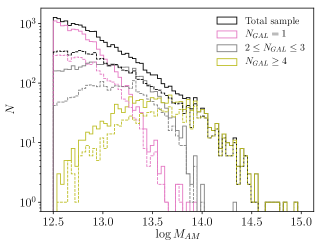
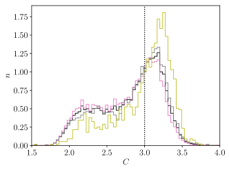
Figure 1: Upper panel and middle panel: Distribution of masses and redshift of the analysed samples of groups. Solid and dashed lines correspond to the mass distributions obtained for the total and $C-$sample, respectively. Dotted vertical in the middle panel indicates the $z=0.13$ limit used to select high- and low-redshift samples. Lower panel: Normalised distribution of the concentration index for the total sample of the groups analysed. The dotted vertical line at $C=3.0$ indicates the concentration value adopted to select the $C-$sample of groups. For all the panels the coloured distributions correspond to different membership bins selected according to $N_{\text{GAL}}$.

We use the publicly available galaxy group catalogue obtained through the identification algorithm by Rodriguez2020, which combines friends-of-friends (FOF, Huchra1982) and halo-based methods (Yang2005). This group finder aims to identify gravitationally bound galaxy systems with at least one bright galaxy, a galaxy with an absolute $r-$band, $M_{r}$ , magnitude lower than $-19.5$. By so doing, we consider galaxy systems dominated by a central galaxy with fainter members that were not included in the spectroscopic catalogue. Briefly, the algorithm performs an iterative identification procedure that consists in two parts. First, all the galaxies with $M_{r}<-19.5$ are linked using a FOF method based on spatial separation criteria following the prescriptions in Merchan2002; Merchan2005. After this step, group candidates with at least one bright member are obtained.

Once the catalogue of potential groups is obtained, the membership assignment is optimised by applying a halo-based group finder following Yang2005; Yang2007. In this step, the algorithm computes a three-dimensional density contrast in redshift space, taking into account a characteristic luminosity calculated according to the potential galaxy members. The characteristic luminosity, $L_{\text{gr}}$, associated to each group can be estimated from the luminosity of their galaxy members plus a correction that takes into account the incompleteness due to the limiting magnitude of the observational data (Moore1993).

Considering each group characteristic luminosity a halo mass is assigned, $M_{\text{AM}}$, performing an abundance matching technique on luminosity (e.g., Vale2004; Kravtsov2004; Tasitsiomi2004; Conroy2006), which assumes a one-to-one relation between the mass and the luminosity. Taking this into account, masses are assigned after matching the rank orders of the halo masses and their characteristic luminosity for a given comoving volume, considering the Warren2006 halo mass function. A caveat is introduced at this stage, since the assumed halo mass function is cosmology dependent, which could introduce some biases when using the density distribution of groups binned in mass as cosmological probes. Nonetheless, masses can be easily re-computed using another cosmology. It is important to highlight that, in spite this approach is based in the assumption of a one-to-one relation between the mass and the luminosity, masses are assigned after ranking the groups according to the computed $L_{\text{gr}}$ and then matching the obtained distribution with the predicted taking into account the halo mass function.

After the mass assignment the algorithm computes the three-dimensional density contrast assuming that the distribution of galaxies in phase space follows that of the dark matter particles and adopting a Navarro–Frenk–White (NFW) profile to compute the projected density. The density contrast is estimated at the position of each potential member and only the galaxies that are located above a given threshold are considered as belonging to the system. Taking into account the new membership assignment, a new characteristic luminosity is computed and the algorithm iterates until convergence in the number of members, $N_{\text{GAL}}$.

Galaxy groups are obtained by applying the algorithm to the spectroscopic galaxy catalogue provided by the SDSS-DR12. The catalogue includes $367370$ groups spanning from $z\sim 0.02$ up to $z=0.3$; of which $302392$ with one member, $11943$ with four or more, and a $1386$ with ten or more members. Besides the mass estimate, $M_{\text{AM}}$, assigned during the identification procedure, the catalogue also provides for the groups with $N_{\text{GAL}}\geq 4$ the projected LOS velocity dispersion of the group, $\sigma_{V}$ and a dynamical mass estimate, $M_{vir}$, computed following Merchan2002, according to $\sigma_{V}$ and the position of each member.

We restrict the sample to the clusters that are included within the sky-coverage of the lensing catalogues. We also include in the analysis only the groups with $\log{M_{\text{AM}}/(h^{-1}M_{\odot})}>12.5$, to ensure we are considering group-scale halos, and within a redshift range of $0.05<z<0.2$. The lower limit in the redshift is selected considering that the lensing signal decreases for groups at lower redshifts and the higher limit is selected taking into account that the sample of groups with $N_{\text{GAL}}\geq 4$ extends up to $z\sim 0.23$. Applying these criteria, the total sample analysed comprises of $18030$ systems, $\sim 63\%$ of these are groups with $N_{\text{GAL}}=1$ and $1537$ have more than $4$ members ($N_{\text{GAL}}\geq 4$). We have considered a subsample of these groups, hereafter $C-$sample, taking into account the morphology of the BGM according to the SDSS concentration index, $C$. This parameter is usually adopted to separate early- and late-type galaxies samples and is defined as $C\equiv r_{90}/r_{50}$ (where $r_{90}$ and $r_{50}$ are the radii enclosing $90\%$ and $50\%$ of the $r-$band Petrosian flux, respectively). A sample of galaxies with $C>2.6$ is expected to include $75\%$ of early type galaxies (Strateva2001). Therefore, we define the $C-$sample including groups with their BGM having $C\geq 3.0$, which roughly corresponds to the median value of the concentration distribution for the total sample of groups analysed. Furthermore, in order to explore the effects of variations of scaling relation between mass proxies for group samples with different mean redshift, we select two samples: a low-redshift ($z<0.13$), and a high-redshift ($z\geq 0.13$) sample. In Fig. 1 we show the halo mass distribution, $\log{M_{\text{AM}}}$, for the total sample, the $C-$sample and other subsamples selected according to the number of members ($N_{\text{GAL}}=1$, $2\leq N_{\text{GAL}}\leq 3$ and $N_{\text{GAL}}\geq 4$). We also show the concentration index distribution for the group sample analysed. As it can be noticed, the concentration cut mainly discard low richness systems and so, bias the mass distribution to higher values.

2.3 Simulated data

As will be detailed in Sec. 3, for our lensing analysis we assume that the halo centre can be well approximated by the BGM position. In order to test the effects of a wrong membership assignment introduced by the identification algorithm, we use a mock catalogue employing synthetic galaxies extracted from a semi-analytic model of galaxy formation applied on top of the Millennium Run Simulation I (Springel2005).

The Millennium Simulation is a cosmological N-body simulation that evolves more than 10 billion dark matter particles in a 500$h^{-1}$Mpc periodic box, using a comoving softening length of 5$h^{-1}$ kpc. This simulation offers high spatial and time resolution within a large cosmological volume. This is a dark matter only simulation, but there are different models to populate halos with galaxies. One of these is the semi-analytic galaxy formation model developed by Guo2010, that we use to build our synthetic galaxy catalogue.

We construct our catalogue following the same procedure as in Rodriguez2015 and Rodriguez2020. Since the Millenium simulation box is periodic, we place the observer at the coordinate origin and repeat the simulated volume until we reach the SDSS volume. The redshifts were obtained using the distances to the observer and taking into account the distortion produced by proper motions. Finally, to mimic SDSS we impose the same upper apparent magnitude threshold of this catalogue and we use the mask to perform the same angular selection function of the survey.

We obtain the mock galaxy group catalogue by applying Rodriguez2020 identification algorithm with the same criteria as described in the previous subsection. In order to compute the shift of the centres due to the identification process, we match the halo to each group identified by our method, by looking for the maximum number of members in common. Then we compute the fraction of groups for which the brightest galaxy is located at the halo centre.

3 Lensing mass estimates

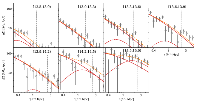
Figure 2: Contrast density profiles for the subsamples selected from the total sample in the whole richness and redshift range ($N_{\text{GAL}}\geq 1$ and $0.05\leq z<0.2$). Labels indicate the $\log{M_{\text{AM}}}$ bin. Dashed orange lines corresponds to the total fitted profile (Eq. 6) and solid and dashed red lines corresponds to the centred, $\Delta\Sigma_{cen}$ (Eq. 7), and the miscentring terms, $\Delta\Sigma_{mis}$ (Eq. 12), respectively. Offset distributions are computed according to Eq. 9. Vertical dashed lines correspond to the upper limit in the projected radius adopted in the fitting procedure.

Figure 3: Idem as in Fig. 2 but for subsamples selected from the $C-$sample in the whole richness and redshift range ($N_{\text{GAL}}\geq 1$ and $0.05\leq z<0.2$).

3.1 Adopted formalism

The weak gravitational lensing effect exerted by the mass distribution associated to galaxy groups, produces a shape distortion of the background galaxies, resulting in an alignment of these galaxies in a tangential orientation with respect to the group centre. The introduced distortion by the lensing effect, can be quantified by the shear parameter, $\gamma=\gamma_{1}+i\gamma_{2}$, and can be estimated according to the measured ellipticity of background galaxies. The observed ellipticity results in a combination of the galaxy intrinsic shape and the introduced by the lensing effect. Assuming that the galaxies are randomly orientated in the sky, the shear can be estimated by averaging the ellipticity of many sources, $\langle e\rangle={\gamma}$. The noise introduced by the intrinsic shape of the sources can be reduced by using stacking techniques, which consists on combining several lenses which increase the density of sources. Stacking techniques effectively increase the signal-to-noise ratio of the shear measurements, allowing us to derive reliable average mass density distributions of the combined lenses (e.g. Leauthaud2017; Simet2017; Chalela2018; Pereira2020).

For a given projected mass density distribution, the azimuthally averaged tangential component, $\gamma_{\rm{t}}$, of the shear can be related with the mass density contrast distribution following (Bartelmann1995):

$$\gamma_{\rm{t}}(r)\times\Sigma_{\rm crit}=\bar{\Sigma}(<r)-\Sigma(r)\equiv\Delta\Sigma(r),$$ (1)

where we have defined the surface mass density contrast $\Delta\Sigma$. Here $\gamma_{\rm{t}}(r)$ is the tangential component of the shear at a projected distance $r$ from the centre of the mass distribution, $\Sigma(r)$ is the projected mass surface density distribution, and $\bar{\Sigma}(<r)$ is the average projected mass distribution within a disk at projected distance $r$. $\Sigma_{\rm crit}$ is the critical density defined as:

$$\Sigma_{\rm{crit}}=\dfrac{c^{2}}{4\pi G}\dfrac{D_{OS}}{D_{OL}D_{LS}},$$ (2)

where $D_{OL}$, $D_{OS}$ and $D_{LS}$ are the angular diameter distances from the observer to the lens, from the observer to the source and from the lens to the source, respectively.

To model the surface density distribution of the halo, $\Sigma$, we use the usual NFW profile (Navarro97). This model depends on two parameters: the radius that encloses the mean density equal to 200 times the critical density of the Universe, $R_{200}$, and a dimensionless concentration parameter, $c_{200}$. The density profile is defined as:

$$\rho(r)=\dfrac{\rho_{\rm crit}\delta_{c}}{(r/r_{s})(1+r/r_{s})^{2}},$$ (3)

where $r_{s}$ is the scale radius, $r_{s}=R_{200}/c_{200}$, $\rho_{\rm crit}$ is the critical density of the Universe at the mean redshift of the sample of stacked galaxy groups, $\langle z\rangle$, and $\delta_{c}$ is the characteristic overdensity of the halo:

$$\delta_{c}=\frac{200}{3}\dfrac{c_{200}^{3}}{\ln(1+c_{200})-c_{200}/(1+c_{200})}.$$ (4)

We compute $\langle z\rangle$ by averaging the group sample redshifts, weighted according to the number of background galaxies considered for each group. The mass within $R_{200}$ can be obtained as $M_{200}=200\,\rho_{\rm crit}(4/3)\pi\,R_{200}^{3}$. The lensing formula adopted to model this profile is described by Wright2000. In the fitting procedure we use a fixed mass-concentration relation $c_{200}(M_{200},z)$, derived from simulations by Duffy2008:

$$c_{200}=5.71\left(M_{200}/2\times 10^{12}h^{-1}\right)^{-0.084}(1+\langle z\rangle)^{-0.47}.$$ (5)

This approach is applied since the concentration parameter mainly affects the slope in the inner regions of the profile and therefore is poorly constrained. Nevertheless, as shown in previous studies the particular choice of this relation does not have a significant impact on the final mass values, which have uncertainties dominated by the noise of the shear profile (Rodriguez2020b).

To compute the profiles we adopt as the group centre, the position of the BGM. The offset distribution between these galaxy-based centres and the true halo centre can be described by considering two group sample populations: well-centred and miscentred groups (Yang2006; Johnston2007; Ford2014; Yan2020). This miscentring affects the observed shear profile by flattening the lensing signal at the inner regions. We consider the miscentring effect in our analysis by modelling the contrast density distribution taking into account two terms:

$$\Delta\Sigma=p_{\text{cc}}\Delta\Sigma_{cen}+(1-p_{\text{cc}})\Delta\Sigma_{mis},$$ (6)

where $\Delta\Sigma_{cen}$ and $\Delta\Sigma_{mis}$ correspond to the contrast density distribution for a perfectly centred, and a miscentred dark matter distribution, respectively, and $p_{\text{cc}}$ is the fraction of well-centred clusters. $\Delta\Sigma_{cen}$ is obtained as:

$$\Delta\Sigma_{cen}(r)=\bar{\Sigma}(<r)-\Sigma(r).$$ (7)

The miscentring term, $\Delta\Sigma_{mis}$, is modelled following Yang2006; Johnston2007; Ford2014. An axis-symmetric surface mass density distribution whose centre is offset by $r_{s}$, with respect to the adopted centre in the lens plane, results in a projected average density profile given by:

$$\Sigma(r|r_{s})=\frac{1}{2\pi}\int^{2\pi}_{0}\Sigma\left(\sqrt{r^{2}+r^{2}_{s}+2rr_{s}\cos{\theta}}\right)d\theta.$$ (8)

The fraction of miscentered groups is expected to be shifted following a Gaussian distribution, therefore the projected offsets can be modelled according to a Rayleigh distribution:

$$P(r_{s})=\frac{r_{s}}{\sigma^{2}_{\text{off}}}\exp{\left(-\frac{1}{2}\frac{r^{2}_{s}}{\sigma^{2}_{\text{off}}}\right)}.$$ (9)

Alternatively, we have also considered a Gamma function with shape parameter $k=2$ to model the offset distribution:

$$P(r_{s})=\frac{r_{s}}{\sigma^{2}_{\text{off}}}\exp{\left(-\frac{r_{s}}{\sigma_{\text{off}}}\right)}.$$ (10)

We consider this model based on the recent work of Yan2020 where they study the miscentring effect by considering different proxies using hydrodynamic simulations.

Taking this into account, the miscentred density can be computed as follows:

$$\Sigma_{mis}(r)=\int_{0}^{\infty}P(r_{s})\Sigma(r|r_{s})dr,$$ (11)

such that the miscentring term for the density contrast profile is:

$$\Delta\Sigma_{mis}(r)=\bar{\Sigma}_{miss}(<r)-\Sigma_{mis}(r).$$ (12)

3.2 Computed estimator and fitting procedure

We compute the density contrast distribution profiles by averaging the tangential ellipticity component of the background galaxies of each group considered in the stacking, as:

$$\Delta\tilde{\Sigma}(r)=\frac{\sum_{j=1}^{N_{L}}\sum_{i=1}^{N_{S,j}}\omega_{LS,ij}\Sigma_{{\rm crit},ij}e_{{\rm t},ij}}{\sum_{j=1}^{N_{L}}\sum_{i=1}^{N_{S,j}}\omega_{LS,ij}},$$ (13)

where $\omega_{LS,ij}$ is the inverse variance weight computed according to the weight, $\omega_{ij}$, given by the $lens$fit algorithm for each background galaxy, $\omega_{LS,ij}=\omega_{ij}/\Sigma^{2}_{{\rm crit},ij}$. $N_{L}$ is the number of galaxy groups considered for the stacking and $N_{S,j}$ the number of background galaxies located at a distance $r\pm\delta r$ from the $j$th group. $\Sigma_{{\rm crit},ij}$ is the critical density for the $i-$th background galaxy of the $j-$th group. The inner regions of the profile could be affected by a stellar mass contribution of the central galaxies. Moreover, these regions are more affected by the background selection and an increased scatter to low sky area in the inner regions. Taking these facts into account, we obtain the profiles by binning the background galaxies in 15 non-overlapping log-spaced $r$ bins, from $300h^{-1}$kpc up to $5h^{-1}$Mpc.

Errors in the photometric redshifts can led to the inclusion of foreground or galaxy members in the background galaxy sample. These galaxies are unlensed and result in an underestimated density contrast, which is called as the dilution effect. In order to take this effect into account, the $\Delta\tilde{\Sigma}$ measurement can be boosted to recover the corrected signal by using the so-called boost-factor (Kneib2003; Sheldon2004; Applegate2014; Hoekstra2015; Simet2017; Leauthaud2017; Melchior2017; McClintock2019; Varga2019; Pereira2020): $1/(1-f_{cl})$, where $f_{cl}$ is the cluster contamination fraction and it is expected to be higher in the inner radial bins where the contamination by cluster members is more significant. We compute $f_{cl}$ by using a similar approach as the presented in Hoekstra2007. Since a non-contaminated background galaxy sample will present a constant density for all the considered radial bins, by computing the excess in the density at each considered radial bin we obtain an estimated value of $f_{cl}$. This excess is computed taking into account the background galaxy density obtained for the last radial bin at $5h^{-1}$Mpc, where the contamination of unlensed galaxies is expected to be negligible. By doing so, we obtain the $f_{cl}(r)$ fraction which is included in the analysis. The inclusion of the boost-factor in the analysis result in higher mass estimates by a $\sim 10\%$ ($\sim 25\%$) for the lowest (highest) mass bin sample of groups.

In order to estimate the group halo masses we fit the computed profiles with the adopted model (Eq. 6) considering the two free parameters, $p_{\text{cc}}$ and $M_{\text{WL}}$ (where $M_{\text{WL}}$ is the $M_{200c}$ mass). We fix the width of the offset distributions, $\sigma_{\text{off}}$, in terms of the radius, $R_{AM}$, which is the $R_{200}$ radius estimated from the abundance matching mass $M_{\text{AM}}$, which are expected to be related (Simet2017). Thus, we set $\sigma_{\text{off}}=0.4\times R_{AM}$ in Eq. 9 according to the results presented in Simet2017. On the other hand, the offset dispersion in Eq. 10 is given by $\sigma_{\text{off}}=0.3\times R_{AM}$ from Yan2020. This approach is similar to the one applied in the fitting procedure of previous stacking analysis (Simet2017; Pereira2018; McClintock2019; Pereira2020) in which $\sigma_{\text{off}}$ is fitted considering a radius computed according to the richness estimator. Although this parameter is fixed taking into account the radius derived according to the $M_{\text{AM}}$ mass estimate, we also try fitting this parameter together with the mass estimate, $\sigma_{\text{off}}=0.4\times R_{WL}$ and $\sigma_{\text{off}}=0.3\times R_{WL}$. The resultant fitted parameters, $p_{\text{cc}}$ and $M_{\text{WL}}$, were in agreement with the previous estimates but less constrained. Therefore our final masses do not strongly depend on $\sigma_{\text{off}}$. We highlight that the fitted miscentring term can be also affected by the adopted concentration, $c_{200}$, since this parameter impacts in the slope profile. We also neglect the contribution of the 2-halo term, introduced by the contribution of neighbouring halos, by fitting the profiles up to a limiting projected radius of $R_{OUT}$. This radius is estimated according to the relation presented by Simet2017 to compute the upper limit radius taking into account $M_{\text{AM}}$. For the highest mass bins considered in the analysis, where the lack of modelling of the 2-halo term can biases the lensing mass estimates, we adopt a more restrictive limiting radius of $2.5h^{-1}$Mpc. Thus, all the profiles are fitted up to $\min(R_{OUT},2.5h^{-1}$Mpc).

We constrain our free parameters, $p_{\text{cc}}$ and $M_{\text{WL}}$, by using the Markov chain Monte Carlo (MCMC) method, implemented through emcee python package (Foreman2013) to optimise the log-likelihood function for the density contrast profile, $\ln{\mathcal{L}}(\Delta\Sigma|r,M_{\text{WL}},p_{\text{cc}})$. We fit the data by using 10 walkers for each parameter and 500 steps, considering flat priors for the mass and the fraction of well-centred groups, $11.5<\log(M_{\text{WL}}/(h^{-1}M_{\odot}))<16$ and $0.2<p_{\text{cc}}<1.0$. We adopt as the best fit parameters the median value of the posterior distributions and the correspondent errors are based on the differences between the median and the $16^{th}$ and $84^{th}$ percentiles, without considering the first 100 steps of each chain. We show in Fig. 2 and 3 the computed profiles together with the fitted models, for the subsamples selected in $\log M_{\text{AM}}$ bins from the total sample and the $C-$sample, respectively.

4 Results

In this section, we first discuss the adopted miscentring modelling and compare the lensing results to numerical simulations. Then, we compare the derived lensing masses to the mass estimates provided by the group catalogue, $M_{\text{AM}}$, computed according to the abundance matching assignment. We also study biases in group masses for the different subsamples selected considering the group richness and redshift. Finally, for the groups with $N_{\text{GAL}}\geq 4$, we compare derived lensing mass estimates to the projected LOS velocity dispersion, $\sigma_{V}$.

In order to study the relation between the abundance matching masses and the lensing estimates, we split the total sample and the $C-$sample of groups in seven $\log{M_{\text{AM}}}$ bins from $10^{12.5}h^{-1}M_{\odot}$ up to $10^{15}h^{-1}M_{\odot}$. We also obtain the lensing masses considering the richness subsamples defined in subsection 2.2 and high- and low-redshift subsamples. In Table 1 and LABEL:table:results we describe the selection criteria together with the best fitted parameters for the samples selected according to the richness and redshift, respectively. In Appendix LABEL:app:corner we show the 2D posterior probability distributions for the total sample. We also show in Appendix LABEL:app:lum the characteristic luminosity distributions, their medians and 15- and 85-th percentiles for each considered bin. Derived lensing masses for the sub-samples range from $3\times 10^{12}h^{-1}M_{\odot}$ to $5\times 10^{14}h^{-1}M_{\odot}$. Therefore, our analysis spans over a wide range of halo masses. We further discuss the results obtained in the next subsections.

Table 1: Fitted parameters for the analysed galaxy groups in the whole redshift range ($0.05\leq z<0.2$).

Richness	$\log{M_{\text{AM}}}$	Total sample			$C-$sample
selection		$N_{L}$	$M_{\text{WL}}$	$p_{\text{cc}}$	$N_{L}$	$M_{\text{WL}}$	$p_{\text{cc}}$
	[$\log{(h^{-1}M_{\odot})}$]		[$10^{13}h^{-1}M_{\odot}$]			[$10^{13}h^{-1}M_{\odot}$]
$N_{\text{GAL}}\geq 1$	$[12.5,13.0)$	$12647$	$0.31_{-0.07}^{+0.05}$	$0.57_{-0.25}^{+0.26}$	$4421$	$0.60_{-0.14}^{+0.10}$	$0.62_{-0.28}^{+0.26}$
	$[13.0,13.3)$	$3093$	$0.95_{-0.15}^{+0.13}$	$0.90_{-0.14}^{+0.08}$	$1551$	$1.48_{-0.22}^{+0.19}$	$0.91_{-0.15}^{+0.07}$
	$[13.3,13.6)$	$1406$	$1.81_{-0.28}^{+0.27}$	$0.75_{-0.18}^{+0.15}$	$832$	$2.14_{-0.39}^{+0.30}$	$0.85_{-0.17}^{+0.11}$
	$[13.6,13.9)$	$571$	$3.4_{-0.5}^{+0.5}$	$0.83_{-0.15}^{+0.12}$	$380$	$2.80_{-0.63}^{+0.51}$	$0.86_{-0.15}^{+0.10}$
	$[13.9,14.2)$	$236$	$4.5_{-0.8}^{+0.9}$	$0.88_{-0.16}^{+0.09}$	$178$	$5.3_{-1.0}^{+1.0}$	$0.89_{-0.16}^{+0.08}$
	$[14.2,14.5)$	$68$	$21_{-4}^{+4}$	$0.50_{-0.14}^{+0.17}$	$50$	$18_{-4}^{+5}$	$0.47_{-0.15}^{+0.16}$
	$[14.5,15.0)$	$9$	$61_{-25}^{+19}$	$0.32_{-0.08}^{+0.14}$	$7$	$66_{-23}^{+19}$	$0.32_{-0.09}^{+0.17}$
$N_{\text{GAL}}=1$	$[12.5,12.9)$	$8815$	$0.34_{-0.09}^{+0.07}$	$0.52_{-0.28}^{+0.25}$	$2894$	$0.56_{-0.15}^{+0.14}$	$0.65_{-0.28}^{+0.25}$
	$[12.9,13.1)$	$1703$	$0.70_{-0.20}^{+0.17}$	$0.75_{-0.28}^{+0.16}$	$810$	$1.35_{-0.39}^{+0.25}$	$0.79_{-0.28}^{+0.16}$
	$[13.1,13.5)$	$748$	$1.70_{-0.40}^{+0.37}$	$0.82_{-0.20}^{+0.12}$	$442$	$2.17_{-0.51}^{+0.45}$	$0.84_{-0.20}^{+0.12}$
$2\leq N_{\text{GAL}}\leq 3$	$[12.5,13.5)$	$4843$	$0.56_{-0.11}^{+0.12}$	$0.57_{-0.25}^{+0.18}$	$2069$	$1.12_{-0.22}^{+0.20}$	$0.73_{-0.25}^{+0.18}$
	$[13.5,14.5)$	$357$	$3.8_{-0.6}^{+0.7}$	$0.79_{-0.18}^{+0.07}$	$237$	$3.7_{-0.7}^{+0.7}$	$0.90_{-0.18}^{+0.07}$
$N_{\text{GAL}}\geq 4$	$[12.5,13.8)$	$1113$	$1.29_{-0.31}^{+0.28}$	$0.68_{-0.22}^{+0.14}$	$639$	$1.31_{-0.36}^{+0.33}$	$0.81_{-0.22}^{+0.14}$
	$[13.8,14.2)$	$348$	$3.9_{-0.6}^{+0.7}$	$0.90_{-0.14}^{+0.07}$	$255$	$4.8_{-0.8}^{+0.7}$	$0.90_{-0.14}^{+0.07}$
	$[14.2,15.5)$	$75$	$28_{-5}^{+4}$	$0.42_{-0.10}^{+0.17}$	$56$	$26_{-5}^{+4}$	$0.36_{-0.10}^{+0.17}$

Notes. Columns: (1) Richness range of the selected sub-samples (2) Selection criteria according to the abundance matching mass, $M_{\text{AM}}$; (3), (4) and (5) number of groups considered in the stacked sample and fitted parameters, $M_{\text{WL}}$ and $p_{\text{cc}}$, for the total sample of groups. (6), (7) and (8) same for the groups included in the $C-$sample.