The distribution of localization measures of chaotic eigenstates in the stadium billiard

Abstract

The localization measures $A$ (based on the information entropy) of localized chaotic eigenstates in the Poincaré-Husimi representation have a distribution on a compact interval $[0,A_{0}]$, which is well approximated by the beta distribution, based on our extensive numerical calculations. The system under study is the Bunimovich’ stadium billiard, which is a classically ergodic system, also fully chaotic (positove Lyapunov exponent), but in the regime of a slightly distorted circle billiard (small shape parameter $\varepsilon$) the diffusion in the momentum space is very slow. The parameter $\alpha=t_{H}/t_{T}$, where $t_{H}$ and $t_{T}$ are the Heisenberg time and the classical transport time (diffusion time), respectively, is the important control parameter of the system, as in all quantum systems with the discrete energy spectrum. The measures $A$ and their distributions have been calculated for a large number of $\varepsilon$ and eigenenergies. The dependence of the standard deviation $\sigma$ on $\alpha$ is analyzed, as well as on the spectral parameter $\beta$ (level repulsion exponent of the relevant Brody level spacing distribution). The paper is a continuation of our recent paper (B. Batistić, Č. Lozej and M. Robnik, Nonlinear Phenomena in Complex Systems 21, 225 (2018)), where the spectral statistics and validity of the Brody level spacing distribution has been studied for the same system, namely the dependence of $\beta$ and of the mean value $<A>$ on $\alpha$.

I Introduction

Quantum chaos (or more generally, wave chaos) is the study of phenomena in the quantum domain, which correspond to the classical chaos. Thus, in the short wavelength approximation we consider the dynamics of rays as the lowest order approximation of the solution of the underlying wave equation, while in the next order we have to consider the wave nature of the solutions, describing the interference effects. The classical-quantum correspondence is thus, for example, entirely analogous to the correspondence between the Gaussian ray optics and the solutions of the Maxwell equation as the governing wave equation. The major technique to bridge the classical and quantum phenomena is the semiclassical mechanics. For an introduction to quantum chaos see the books by Stöckmann Stöckmann (1999) and Haake Haake (2001), and a recent review Robnik (2016).

The quantum localization (or dynamical localization) of classical chaotic diffusion in the time-dependent domain is one of the most important fundamental phenomena in quantum chaos, discovered and studied first in the quantum kicked rotator Casati et al. (1979); Chirikov et al. (1981, 1988); Izrailev (1990) by Chirikov, Casati, Izrailev, Shepelyansky, Guarneri and many others, as an example of a time-periodic Floquet system, whose behaviour is quite typical. See also papers by Izrailev Izrailev (1988, 1989) and his review Izrailev (1990). Intuitively and qualitatively, the quantum diffusion does follow the classical chaotic diffusion, but only up to the Heisenberg time (also called break time), where it stops due to the (typically destructive) interfercence effects. The Heisenberg time $t_{H}=2\pi\hbar/\Delta E$, where $\Delta E$ is the mean energy level spacing (reciprocal energy level density), is an important time scale in any quantum system with the discrete energy spectrum. It is the time scale up to which the discreteness of the evolution operator is not resolved. Note that $t_{H}$ and $\Delta E$ are related through a Fourier transform of the evolving wave functions.

In the time-independent domain the quantum localization is manifested in the localized chaotic eigenstates. In the case of the quantum kicked rotator, for example, one sees the exponentially localized eigenstates in the dimensionless space of the angular momentum quantum number. For an extensive review see Izrailev (1990). This phenomenon is closely related to the Anderson localization in one dimensional disordered lattices as shown for the first time by Fishman, Grempel and Prange Fishman et al. (1982), and later discussed and studied by many others Stöckmann (1999); Haake (2001).

Billiards are very convenient model systems, as they are simple but nevertheless exhibit all generic properties of chaotic Hamiltonian systems. The dynamical localization in billiards has been reviewed by Prosen Prosen (2000). We study the localization properties of the chaotic eigenstates, which means studying the structure of the Wigner functions (which are real but not positive definite) or better the Husimi functions (which are real and positive definite). The latter ones can be considered as a probability density. The separation of chaotic and regular eigenstates is done by comparing the classical phase space with the structure of their Wigner or Husimi functions. The control parameter governing the degree of quantum localization is

$$\alpha=\frac{t_{H}}{t_{T}}$$ (1)

where $t_{T}$ is the dominating classical transport time (or diffusion time, or ergodic time). Batistić and Robnik Batistić and Robnik (2013a) have recently studied the localization of chaotic eigenstates in the mixed-type billiard Robnik (1983, 1984), after the separation of the chaotic and regular eigenstates based on such quantum-classical correspondence Batistić and Robnik (2013b). Two localization measures have been introduced, one based on the information entropy denoted by $A$ and used in this paper, and the other one $C$ based on the correlations. They have shown that $A$ and $C$ are linearly related and thus equivalent, which confirms that the definitions are physically sound and useful.

In a recent paper Batistić et al. (2018) we have studied the localization properties of chaotic eigenstates in the stadium billiard of Bunimovich Bunimovich (1979), which is ergodic and chaotic system (positive Lyapunov exponents). Studies of the slow diffusive regime in this system and the related quantum localization were initiated in Ref. Borgonovi et al. (1996), while the detailed aspects of classical diffusion have been investigated in our recent paper Č. Lozej and Robnik (2018), where the classical diffusion has been analyzed in detail, determining the important classical transport time (diffusion time) $t_{T}$.

Another fundamental phenomenon in quantum chaos in the time-independent domain is the statistics of the fluctuations in the energy spectra, which are universal Stöckmann (1999); Haake (2001); Mehta (1991); Guhr et al. (1998); Robnik (1998) for classically fully chaotic ergodic systems (described by the random matrix theories) and for integrable systems (Poissonian statistics). For this to apply one must be in the sufficiently deep semiclassical limit (when $\alpha$ is large enough, $\alpha\gg 1$, which can always be achieved by sufficiently small effective $\hbar$). In the general mixed type systems, in the sufficiently deep semiclassical limit, the spectral statistical properties are determined solely by the type of classical motion, which can be either regular or chaotic Percival (1973); Berry and Robnik (1984); Robnik (1998); Batistić and Robnik (2010, 2013a, 2013b). The level statistics is Poissonian if the underlying classical invariant component is regular. For chaotic extended states the Random Matrix Theory (RMT) applies Mehta (1991), specifically the Gaussian Orthogonal Ensemble statistics (GOE) in case of an antiunitary symmetry. This is the Bohigas-Giannoni-Schmit conjecture Casati et al. (1980); Bohigas et al. (1984), which has been proven only recently Sieber and Richter (2001); Müller et al. (2004); Heusler et al. (2004); Müller et al. (2005, 2009) using the semiclassical methods, the periodic orbit theory developed around 1970 by Gutzwiller (Gutzwiller (1980) and the references therein), an approach initiated by Berry Berry (1985), well reviewed in Stöckmann (1999); Haake (2001).

The classification regular-chaotic can be done by analyzing the structure of eigenstates in the quantum phase space, based on the Wigner functions, or Husimi functions Batistić and Robnik (2013b). Of course, in the stadium billiard all eigenstates are of the chaotic type, but can be strongly localized if $\alpha$ is small enough, $\alpha\ll 1$.

The most important spectral statistical measure is the level spacing distribution $P(S)$, assuming spectral unfolding such that $\left<S\right>=1$. For integrable systems and regular levels of mixed type systems $P(S)=\exp\left(-S\right)$, whilst for extended chaotic systems it is well approximated by the Wigner distribution $P(S)=\frac{\pi S}{2}\exp\left(-\frac{\pi}{4}\,S^{2}\right)$. The distributions differ significantly in a small $S$ regime, where there is no level repulsion in a regular system and a linear level repulsion, $P(S)\propto S$, in a chaotic system. Localized chaotic states exhibit the fractional power-law level repulsion $P(S)\propto S^{\beta}$, as clearly demonstrated recently by Batistić and Robnik Batistić and Robnik (2010, 2013a, 2013b).

The weak ($\beta<1$) level repulsion of localized chaotic states is empirically observed, but the whole distribution $P(S)$ is globally theoretically not known. Several different distributions which would extrapolate the small $S$ behaviour were proposed. The most popular are the Izrailev distribution Izrailev (1988, 1989, 1990) and the Brody distribution Brody (1973); Brody et al. (1981). The Brody distribution is a simple generalization of the Wigner distribution. Explicitly, the Brody distribution is

$$P_{B}(S)=cS^{\beta}\exp\left(-dS^{\beta+1}\right),\;\;\;$$ (2)

where

$$c=(\beta+1)d,\;\;\;d=\left(\Gamma\left(\frac{\beta+2}{\beta+1}\right)\right)^{\beta+1}$$ (3)

with $\Gamma(x)$ being the Gamma function. It interpolates the exponential and Wigner distribution as $\beta$ goes from $0$ to $1$. One important theoretical plausibility argument by Izrailev in support of such intermediate level spacing distributions is that the joint level distribution of Dyson circular ensembles can be extended to noninteger values of the exponent $\beta$ Izrailev (1990). The Izrailev distribution is a bit more complicated but has the feature of being a better approximation for the GOE distribution at $\beta=1$. However, recent numerical results show that Brody distribution is slightly better in describing real data Batistić and Robnik (2010, 2013a); Manos and Robnik (2013); Batistić et al. (2013), and is simpler, which is the reason why we prefer and use it.

In the previous paper Batistić et al. (2018) it has been shown that there is a linear functional relation between the level repulsion parameter $\beta$ and the mean localization measure $<A>$ in the stadium billiard, in analogy with the quantum kicked rotator, but different from the above mentioned mixed-type billiard. Also, $\beta$ is a unique function of $\alpha$, which has been discussed for the first time by Izrailev Izrailev (1988, 1989, 1990), where he numerically studied the quantum kicked rotator. His result showed that the parameter $\beta$, which was obtained using the Izrailev distribution, is functionally related to the localization measure defined by the information entropy of the eigenstates in the angular momentum representation. His results were recently confirmed and extended, with the much greater numerical accuracy and statistical significance Manos and Robnik (2013); Batistić et al. (2013). Moreover, in Ref. Batistić and Robnik (2013a) it has been demonstrated that $\beta$ is a unique function of $\left<A\right>$ in the billiard with the mixed phase space Robnik (1983, 1984), but is not linear. Finally, Manos and Robnik Manos and Robnik (2015), have observed that the localization measure in the quantum kicked rotator has a nearly Gaussian distribution, and this was a motivation for the work in the present paper, where we study the distributions of $A$ in the stadium billiard, systematically in almost all regions of interest (determined by the shape parameter $\varepsilon$ and the energy), and also the dependence of its standard deviation on the control parameter $\alpha$, while the dependence of $<A>$ on $\alpha$ as an empirical rational function is already known from our previous paper Batistić et al. (2018).

The paper is organized as follows. In section II we define the system and the Poincaré - Husimi functions. In section III we show examples of Poincaré - Husimi functions and calculate the moments of the distributions of the localization measures $P(A)$. In section IV we analyze the distributions $P(A)$ extensively and in detail, and demonstrate that they are very well decsribed by the beta distribution. In section V we consider the implications of localization for the statistical properties of the energy spectra, in particular for the level spacing distribution. In section VI we conclude and discuss the main results.

II The billiard systems and definition of the Poincaré-Husimi functions

The (shape of the) stadium billiard ${\cal B}$ of Bunimovich Bunimovich (1979) is defined as two semicircles of radius 1 connected by two parallel straight lines of length $\varepsilon$, as shown in Fig. 1. We study the dynamics of a point particle moving freely inside the billiard, and experiencing specular reflection when hitting the boundary. In this section we follow our previous paper Batistić et al. (2018) and go further.

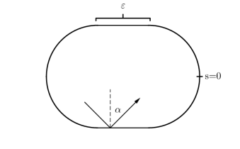
Figure 1: The geometry and notation of the stadium billiard of Bunimovich.

For a 2D billiard the most natural coordinates in the phase space $(s,p)$ are the arclength $s$ round the billiard boundary, $s\in[0,{\cal L}]$, where ${\cal L}$ is the circumference, and the sine of the reflection angle, which is the component of the unit velocity vector tangent to the boundary at the collision point, equal to $p=\sin\alpha$, which is the canonically conjugate momentum to $s$. These are the Poincaré-Birkhoff coordinates. The bounce map $(s_{1},p_{1})\rightarrow(s_{2},p_{2})$ is area preserving Berry (1981), and the phase portrait does not depend on the speed (or energy) of the particle. Quantum mechanically we have to solve the stationary Schrödinger equation, which in a billiard is just the Helmholtz equation

$$\Delta\psi+k^{2}\psi=0$$ (4)

with the Dirichlet boundary conditions $\psi|_{\partial{\cal B}}=0$. The energy is $E=k^{2}$. The important quantity is the boundary function

$$u(s)={\bf n}\cdot\nabla_{{\bf r}}\psi\left({\bf r}(s)\right),$$ (5)

which is the normal derivative of the wavefunction $\psi$ at the point $s$ (${\bf n}$ is the unit outward normal vector). It satisfies the integral equation

$$u(s)=-2\oint dt\;u(t)\;{\bf n}\cdot\nabla_{{\bf r}}G({\bf r},{\bf r}(t)),$$ (6)

where $G({\bf r},{\bf r^{\prime}})=-\frac{i}{4}H_{0}^{(1)}(k|{\bf r}-{\bf r^{\prime}}|)$ is the Green function in terms of the Hankel function $H_{0}(x)$. It is important to realize that the boundary function $u(s)$ contains complete information about the wavefunction at any point ${\bf r}$ inside the billiard by the equation

$$\psi_{m}({\bf r})=-\oint dt\;u_{m}(t)\;G\left({\bf r},{\bf r}(t)\right).$$ (7)

Here $m$ is just the index (sequential quantum number) of the $m$-th eigenstate. Now we go over to the quantum phase space. We can calculate the Wigner functions Wigner (1932) based on $\psi_{m}({\bf r})$. However, in billiards it is advantageous to calculate the Poincaré - Husimi functions. The Husimi functions Husimi (1940) are generally just Gaussian smoothed Wigner functions. Such smoothing makes them positive definite, so that we can treat them somehow as quasi-probability densities in the quantum phase space, and at the same time we eliminate the small oscillations of the Wigner functions around the zero level, which do not carry any significant physical contents, but just obscure the picture. Thus, following Tualle and Voros Tualle and Voros (1995) and Bäcker et al Bäcker et al. (2004), we introduce Batistić and Robnik (2013a, b). the properly ${\cal L}$-periodized coherent states centered at $(q,p)$, as follows

$$c_{(q,p),k}(s) = \sum_{m\in{\bf Z}}\exp\{i\,k\,p\,(s-q+m{\cal L})\}\times$$

$$\exp \left(-\frac{k}{2}(s-q+m{\cal L})^{2}\right).$$

The Poincaré - Husimi function is then defined as the absolute square of the projection of the boundary function $u(s)$ onto the coherent state, namely

$$H_{m}(q,p)=\left|\int_{\partial{\cal B}}c_{(q,p),k_{m}}(s)\;u_{m}(s)\;ds\right|^{2}.$$ (9)

The entropy localization measure of a single eigenstate $H_{m}(q,p)$, denoted by $A_{m}$ is defined as

$$A_{m}=\frac{\exp I_{m}}{N_{c}},$$ (10)

where

$$I_{m}=-\int dq\,dp\,H_{m}(q,p)\ln\left((2\pi\hbar)^{f}H_{m}(q,p)\right)$$ (11)

is the information entropy. Here $f$ is the number of degrees of freedom (for 2D billiards $f=2$, and for surface of section it is $f=1$) and $N_{c}$ is a number of cells on the classical chaotic domain, $N_{c}=\Omega_{c}/(2\pi\hbar)^{f}$, where $\Omega_{c}$ is the classical phase space volume of the classical chaotic component. In the case of the uniform distribution (extended eigenstates) $H=1/\Omega_{C}={\rm const.}$ the localization measure is $A=1$, while in the case of the strongest localization $I=0$, and $A=1/N_{C}\approx 0$. The Poincaré - Husimi function $H(q,p)$ (9) (normalized) was calculated on the grid points $(i,j)$ in the phase space $(s,p)$, and we express the localization measure in terms of the discretized function. In our numerical calculations we have put $2\pi\hbar=1$, and thus we have $H_{ij}=1/N$, where $N$ is the number of grid points, in case of complete extendedness, while for maximal localization we have $H_{ij}=1$ at just one point, and zero elsewhere. In all calculations have used the grid of $400\times 400$ points, thus $N=160000$.

As mentioned in the introduction, the definition of localization measures can be diverse, and the question arises to what extent are the results objective and possibly independent of the definition. Indeed, in reference Batistić and Robnik (2013a), it has been shown that $A$ and $C$ (based on the corelations) are linearly related and thus equivalent. Moreover, we have introduced also the normalized inverse participation ratio $nIPR$, defined as follows

$$nIPR=\frac{1}{N}\frac{1}{\sum_{i,j}H_{ij}^{2}},$$ (12)

for each individual eigenstate $m$. However, because we expect fluctutaions of the localization measures even in the quantum ergodic regime (due to the scars etc), we must perform some averaging over an ensemble of eigenstates, and for this we have chosen $100$ consecutive eigenstates. Then, by doing this for all possible data for the stadium at various $\varepsilon$ and $k$, we ended up with the perfect result that the $nIPR$ and $A$ are linearly related and thus also equivalent, as shown in Fig. 2. In the following we shall use exclusively $A$ as the measure of localization.

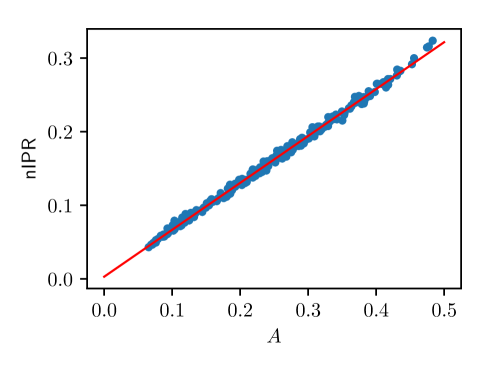
Figure 2: The normalized inverse participation ratio as a localization measure, as a function of $A$. They are linearly related and thus equivalent. The slope is 0.64.

The central object of interest in this paper is the distribution $P(A)$ of the localization measures $A_{m}$ within a certain interval of 1000 consecutive eigenstates indexed by $m$, around some central value $\bar{k}$. We have done this for 17 different values of $\varepsilon$ and for each $\varepsilon$ for 12 different values of $\bar{k}$. Each distribution function $P(A)$, generated by the segment of 1000 consecutive values $A_{m}$, is defined on a compact interval $[0,A_{0}]$. Ideally, according to the above Eqs. (10,11), the maximum value of $A$ should be $1$, if the Husimi function were entirely and uniformly extended. However, this is never the case, as the Husimi functions have zeros and oscillations, and thus we must expect a smaller maximal value, smaller than $1$, which in addition might vary from case to case, depending on $k$ and the grid size. So long as we do not have a theoretical prediction for $A_{0}$, we must proceed empirically. Therefore we have checked several values of $A_{0}$ around $A_{0}=0.7$, and found that the latter value is the best according to several criteria. See also the discussion at the end of section IV.

We shall look at the moments of $P(A)$, namely

$$\left<A\right>=\int_{0}^{A_{0}}A\,P(A)\,dA,\,\,\,\left<A^{2}\right>=\int_{0}^{A_{0}}A^{2}\,P(A)\,dA,$$ (13)

and the standard deviation

$$\sigma=\sqrt{\left<A^{2}\right>-\left<A\right>^{2}}.$$ (14)

For the numerical calculations of the eigenfunctions $\psi_{m}({\bf r})$ and the corresponding energy levels $E_{m}=k_{m}^{2}$ we have used the Vergini-Saraceno method Vergini and Saraceno (1995). Also, we have calculated only the odd-odd symmetry class of solutions.

III Moments of A and examples of Poincaré - Husimi functions

The system parameter governing the localization phenomenon $\alpha=t_{H}/t_{T}$, as introduced in Eq. (1), in a quantum billiard described by the Schrödinger equation (Helmholtz equation) Eq. (4), becomes

$$\alpha=\frac{2k}{N_{T}}.$$ (15)

where $N_{T}$ is the discrete classical transport time, that is the characteristic number of collisions of the billiard particle necessary for the global spreading of the ensemble of uniform in $s$ initial points (excluding the bouncing ball intervals) at zero momentum in the momentum space. This quantity $N_{T}$ can be defined in various ways as discussed in references Batistić et al. (2018); Batistić and Robnik (2013a, b), where the derivation of $t_{T}$, $N_{T}$ and $\alpha$ is given. It is shown there that $N_{T}\propto\varepsilon^{-2.3}$ for small $\varepsilon\leq 0.1$.

The condition for the occurrence of dynamical localization $\alpha\leq 1$ is now expressed in the inequality

$$k\leq\frac{N_{T}}{2},$$ (16)

although the empirically observed transitions are not at all sharp with $\alpha$. More precisely, as in Ref. Batistić et al. (2018), $t_{T}$ is defined as the time at which an ensemble of initial conditions in the momentum space with initial Dirac delta distribution with zero variance reaches a certain fraction of the asymptotic value. In the stadium billiard for small $\varepsilon$ we have a diffusive regime and thus $t_{T}$ can be defined as the diffusion time extracted from the exponential approach of the momentum variance to its asymptotic value $1/3$, as has been recently carefully studied in Ref. Č. Lozej and Robnik (2018). In ref. Batistić et al. (2018) (see Table I) we have published the values of $N_{T}$ for the stadium billiard, for 40 different values of the shape parameter $\varepsilon$, for the criteria $50\%,70\%,80\%,90\%$ of the asymptotic value of the momentum variance $\left<p^{2}\right>$ and for the exponential model.

In Fig. 3 we show the dependence of $\left<A\right>$ on $\alpha$, where $\alpha$ is calculated using $N_{T}$ from the expnential law. The transition from strong localization of small $\left<A\right>$ and $\alpha$ to complete delocalization $\alpha\gg 1$ is quite smooth, over almost two decadic orders of magnitude. As we see, $\left<A\right>$ is well fitted by a rational function of $\alpha$, namely

$$\left<A\right>=A_{\infty}\frac{s\alpha}{1+s\alpha},$$ (17)

where the values of the two parameters are $A_{\infty}=0.58$ and $s=0.19$.

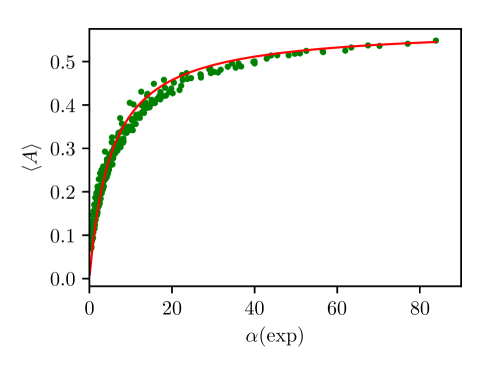
Figure 3: The entropy localization measure $\left<A\right>$ as a function of $\alpha$ fitted by the function (17), based on $N_{T}$ from the exponential diffusion law (see Table I in ref. Batistić et al. (2018)), with $A_{\infty}=0.58$ and $s=0.19$.

In Fig. 4 we show the dependence of $\sigma$ defined in Eq. (14) upon $\alpha$ also using the exponential model for $N_{T}$. The results are functionaly the same when using the other definitions of $N_{T}$, so that we do not show them here.

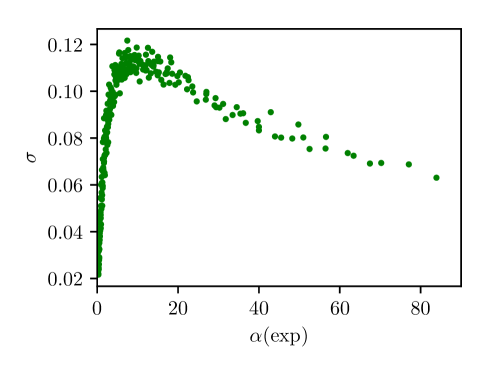
Figure 4: The standard deviation $\sigma$ as a function of the $\alpha$ for variety of stadia of different shapes $\varepsilon$ and energies $E=k^{2}$, as defined in the text.

We see that while $\left<A\right>$ is a monotonically increasing function of $\alpha$ (Fig. 3), the standard deviation $\sigma$ starts at zero, is small for small $\alpha$, but rises sharply, and reaches some maximum at about $\alpha\approx 10$, and then decreases very slowly at large values of $\alpha$. Thus both, the very strongly localized eigenstates, mimicking invariant tori, and the entirely delocalized (ergodic) eigenstates have small spreading $\sigma$ around the mean value $\left<A\right>$. According to the quantum ergodic theorem of Shnirelman Shnirelman (1974) $\sigma$ should tend to zero when $\alpha\rightarrow\infty$, and rescaled $\left<A\right>\rightarrow 1$, but the transition to that regime might be very slow as suggested by Fig. 4. However, it is very difficult to judge this quantitatively, as at large $\alpha$ we have very few physically reliable data points, so it is too early to draw any definite conclusion about the asymptotic behavior at $\alpha\rightarrow\infty$. More numerical efforts are needed, currently not feasible.

The Poincaré - Husimi functions describe the structure of the localized chaotic eigenstates. In Fig. 5 we show some selection of typical Poincaré - Husimi functions for various values of $\varepsilon$ and $k$, and the corresponding $\alpha$. We show only the upper right quadrant $s\in[0,{\cal L}/4]$, $p\in[0,1]$ of the classical phase space, as due to the symmetries (two reflection symmetries and the time reversal symmetry) all four quadrants are equivalent.

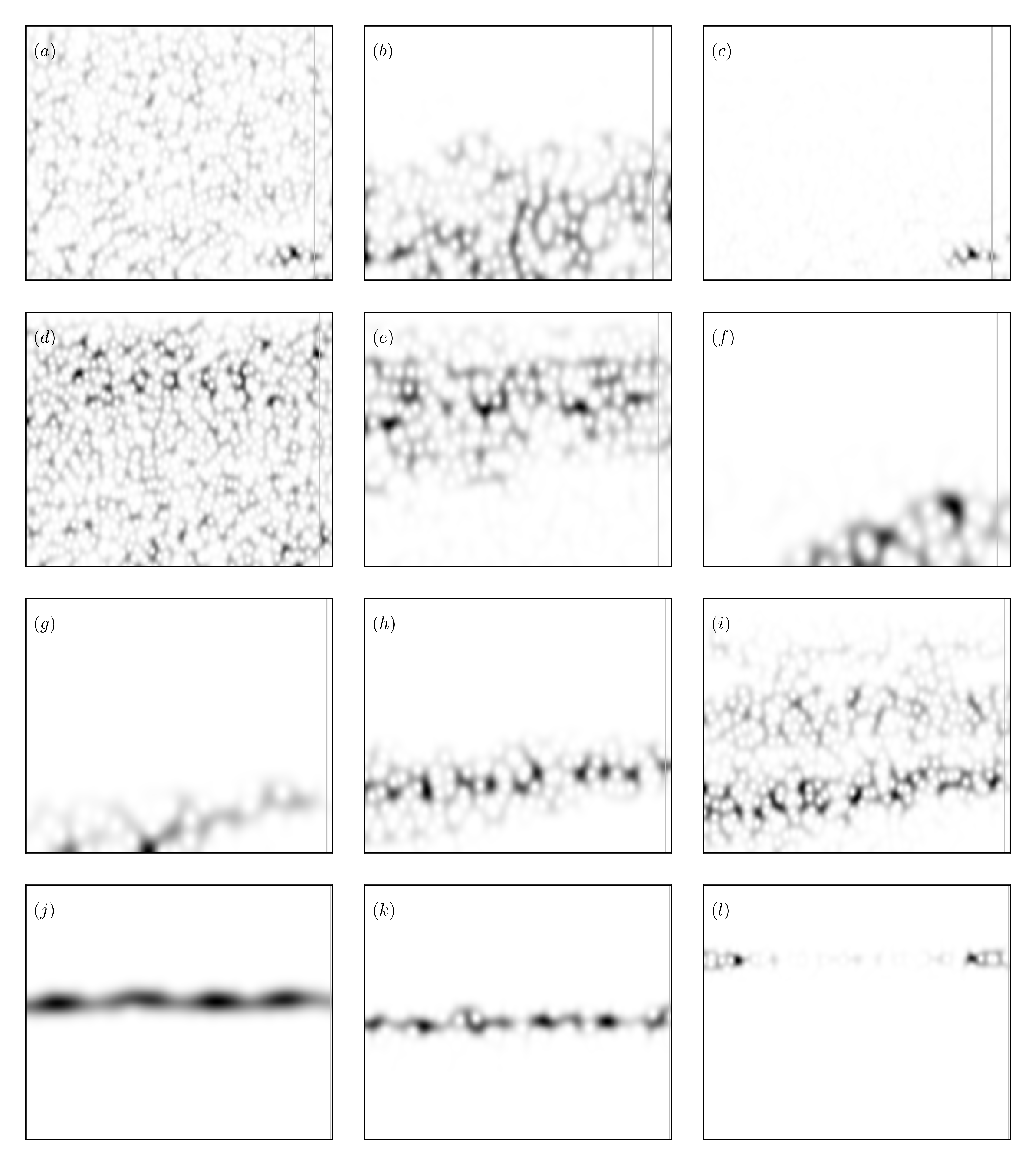
Figure 5: We show plots of Poincaré - Husimi functions for a representative selection of eigenstates: Row (a-c): $\varepsilon=0.2$, $k$: $3720.01170174$, $1480.01417766$ , $3720.01594071$; Row (d-f): $\varepsilon=0.14$, $k$: $3720.01379303$, $1480.03480316$, $640.05384413$; Row (g-i): $\varepsilon=0.06$, $k$: $640.05384413$, $1480.05082005$, $2600.01768874$; Row (j-l): $\varepsilon=0.02$, $k$: $640.00758741$, $1480.03406374$, $3720.00973621$. The thin vertical line denotes the size of the interval $\varepsilon/2$.

At large $\varepsilon$ and fixed $k$, we have small small $N_{T}$ and according to Eq.(15) $\alpha\gg 1$, we observe mainly ergodic eigenstates, in agreement with the quantum ergodic theorem Shnirelman (1974), that is fully extended states, exemplified in (a). Nevertheless, there are some exceptions, asymptotically of measure zero, where we observe partial localization, as shown in (b). Moreover, there can be strongly localized states corresponding to the scaring around and along an unstable periodic orbit as exemplified in (c) and (l). More precisely, the area of scars of eigenfunctions $\psi_{m}({\bf r})$ goes to zero, and the relative number of scarred states goes to zero as $\hbar\rightarrow 0$ or $m\rightarrow\infty$ Heller (1984).

As we decrease $\varepsilon=0.14$ and $\alpha$, thereby increasing $N_{T}$, the degree of localization increases, thus $\left<A\right>$ is decreasing as shown in (d-f). At still lower value of $\varepsilon=0.06$ we see even more strongly localized states exemplified in (g-i). Finally, at the smallest value of $\varepsilon=0.02$ that we considered in our numerical calculations, we see only strongly localized eigenstates mimicking invariant tori, in (j-l), although the system is classically ergodic, but obviously is full of cantori with very low transport permeability.

IV The distributions of the localization measures $A$

In this section we present the central results of this paper, namely the distribution functions of the localization measures $A$. It turns out that each distribution can be very well characterized and described by the so-called beta distribution

$$P(A)=CA^{a}(A_{0}-A)^{b},$$ (18)

where $A_{0}$ is the upper limit of the interval $[0,A_{0}]$ on which $P(A)$ is defined, in our case, as explained in Sec. II, we have chosen $A_{0}=0.7$. The two exponents $a$ and $b$ are positive real numbers, while $C$ is the normalization constant such that $\int_{0}^{A_{0}}P(A)\,dA=1$, i.e.

$$C^{-1}=A_{0}^{a+b+1}B(a+1,b+1),$$ (19)

where $B(x,y)=\int_{0}^{1}t^{x-1}(1-t)^{y-1}dt$ is the beta function. Thus we have

$$\left<A\right>=A_{0}\frac{a+1}{a+b+3},$$ (20)

and for the second moment

$$\left<A^{2}\right>=A_{0}^{2}\frac{(a+2)(a+1)}{(a+b+4)(a+b+3)}$$ (21)

and therefore for the standard deviation $\sigma$ (14),

$$\sigma^{2}=A_{0}^{2}\frac{(a+2)(b+2)}{(a+b+4)(a+b+3)^{2}}.$$ (22)

such that asymptotically $\sigma\approx A_{0}\frac{\sqrt{b+2}}{a}$ when $a\rightarrow\infty$. In the figures 6, 7, 8 we show a selection of typical distributions $P(A)$. In all cases for $A_{0}$ we have chosen $A_{0}=0.7$. By $k_{0}$ we denote the starting value of $k$ intervals on which we calculate the 1000 successive eigenstates. It should be noted that the statistical significance is very high, which has been carefully checked by using a (factor 2) smaller number of objects in almost all histograms, as well as by changing the size of the boxes.

The limiting case $a\rightarrow\infty$ in Eqs.(20,22) comprising the fully extended states in the limit $\alpha\rightarrow\infty$ shows that the distribution tends to the Dirac delta function peaked at $A_{0}$, thus $\sigma=0$ and $P(A)=\delta(A-A_{0})$, in agreement with Shnirelman’s theorem Shnirelman (1974).

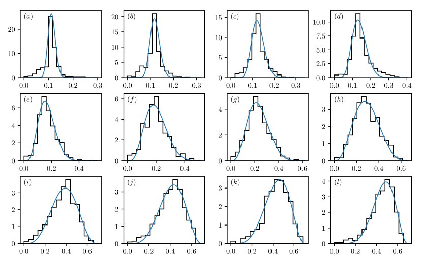
Figure 6: The distributions $P(A)$ of the entropy localization measure $A$ for $k_{0}=640$ and various $\varepsilon$ (from (a) to (l)): 0.02, 0.03, 0.04, 0.05, 0.06, 0.07, 0.08, 0.1, 0.14, 0.16, 0.18, 0.2.

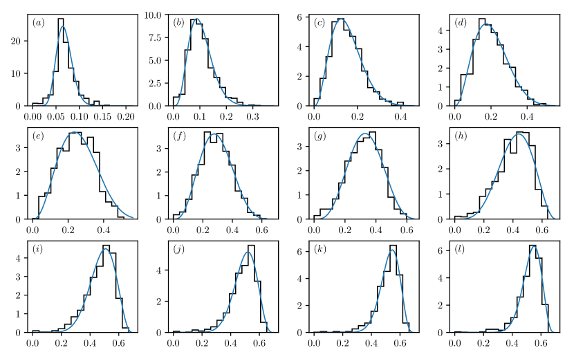
Figure 7: The distributions $P(A)$ of the entropy localization measure $A$ for $k_{0}=2320$ and various $\varepsilon$ (from (a) to (l)): 0.02, 0.03, 0.04, 0.05, 0.06, 0.07, 0.08, 0.1, 0.14, 0.16, 0.18, 0.2.

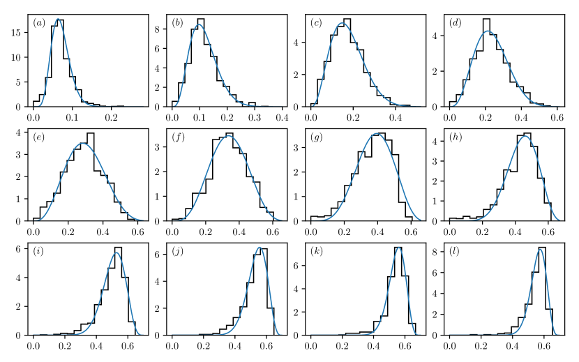
Figure 8: The distributions $P(A)$ of the entropy localization measure $A$ for $k_{0}=3440$ and various $\varepsilon$ (from (a) to (l)): 0.02, 0.03, 0.04, 0.05, 0.06, 0.07, 0.08, 0.1, 0.14, 0.16, 0.18, 0.2.

The figures clearly show that the fit by the beta distribution (18) is excellent, except for few cases at small $\varepsilon$. The corresponding values of $a$, $b$, and $\alpha$ are shown in Table I. The qualitative trend from strong localization to weaker localization or even complete extendedness (ergodicity) with increasing $k_{0}$ and $\varepsilon$ is clearly visible.

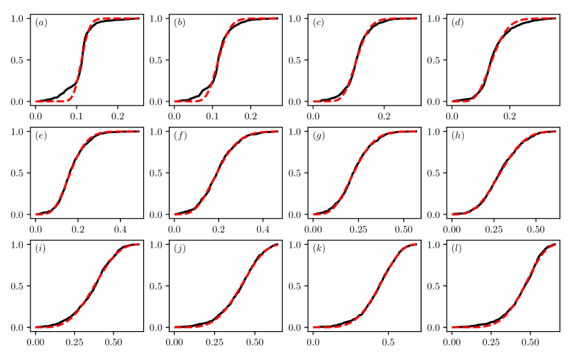
Figure 9: The cumulative distributions $W(A)$ of the entropy localization measure $A$ for $k_{0}=640$ and various $\varepsilon$ (from (a) to (l)): 0.02, 0.03, 0.04, 0.05, 0.06, 0.07, 0.08, 0.1, 0.14, 0.16, 0.18, 0.2. They correspond to Fig. 6. The numerical data are represented by the full line, the dashed one is the best fitting cumulative beta distribution.

The agreement of the distributions $P(A)$, based on 1000 numerical values per histogram, with the empirically found beta distribution, is demonstrated for the cumulative distribution $W(A)$,

$$W(A)=\int_{0}^{A}P(x)\,dx.$$ (23)

in Fig. 9, for $k_{0}=640$ and various $\varepsilon$. The worst case is at small $\varepsilon=0.02$ (a), while the best one is for $\varepsilon=0.2$ (l). The quality of the fit for other values of $\varepsilon$ and $k_{0}$ is much better, comparable to (l). Therefore we may conclude that apart from the smallest $\varepsilon=0.02$, the beta distribution is the semiempirically right description of the distributions $P(A)$.

Parameters of the beta distributions
$a$	$b$	$\alpha$
41.694174	222.486122	0.087593
18.693580	97.355740	0.233279
13.554691	66.554374	0.468864
7.789110	33.474273	0.779063
4.745791	17.092065	1.170018
3.784283	11.147294	1.673203
3.445179	8.128386	2.273535
2.869704	4.433526	3.753666
3.390150	2.806308	7.441860
4.052971	2.581244	9.770992
4.288946	2.245432	12.549020
5.352111	2.401925	15.609756
12.767080	125.817047	0.317525
3.519266	24.397953	0.845635
2.567093	12.051933	1.699634
2.397450	7.362461	2.824102
2.570951	5.339960	4.241316
3.184420	4.989456	6.065359
3.553229	4.183009	8.241563
3.894103	2.440766	13.607038
7.260777	2.884395	26.976744
9.534313	3.451923	35.419847
13.582757	4.012060	45.490196
14.385305	3.975161	56.585366
6.324855	64.722649	0.470814
3.518886	22.076947	1.253873
2.668046	10.146521	2.520147
3.149723	7.293627	4.187462
3.000757	4.566317	6.288848
3.604156	3.959419	8.993464
4.354036	3.582313	12.220249
6.856759	3.788696	20.175953
11.037403	3.748447	40.000000
13.288212	3.566739	52.519084
19.143654	4.832500	67.450980
21.812546	4.992295	83.902439

Table 1: Parameters of the best fitting beta distributions of Figs. 6, 7, 8, successively. $A_{0}$ is fixed, $A_{0}=0.7$.

We should stress that there is of course some arbitrarines in defining $A_{0}$, so long as we do not have a theoretical prediction for its value. So far we have taken $A_{0}=A_{{\rm max}}=0.7$, but nevertheless tried also the choice of $A_{0}$ being the largest member $A$ in each histogram, and found no significant qualitative changes, but only quite minor quantitative differences in the fitting curves of the histograms. In both cases $a$ and $b$ are not unique functions of $\alpha$, while $<A>$ and $\sigma$ are close to being unique functions of $\alpha$ as demonstrated in Figs. 3 and 4, and approximated by a fit in Eq. (17). In Fig. 10 we show in log-lin plot of $a$ and $b$ versus $\alpha$.

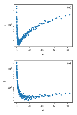
Figure 10: The plot of $a$ and $b$ versus $\alpha$.

V Implications of localization for the spectral statistics

To get a good estimate of $\beta$ we need many more levels (eigenstates) than in calculating $\left<A\right>$. The parameter $\beta$ was computed for 40 different values of the parameter $\epsilon$: $\epsilon_{j}=0.02+0.005\,j$ where $j\in[0,1,\dots,39]$ and on 12 intervals in $k$ space: $(k_{i},k_{i+1})$ where $k_{i}=500+280\,i$ and $i\in[0,1,\dots,11]$. This is $40\times 12=480$ values of $\beta$ altogether. More than $4\times 10^{6}$ energy levels were computed for each $\epsilon$. The size of the intervals in $k$ was chosen to be maximal and such that the Brody distribution gives a good fit to the level spacing distributions of the levels in the intervals, meaning that $\beta$ is well defined.

For each $\beta(\epsilon_{j},(k_{i},k_{i+1}))$ an associated localization measure $\left<A\right>$ was computed on a sample of 1000 consecutive levels around $\bar{k}_{i}=(k_{i}+k_{i+1})/2$, which is a mean value of $k$ on the interval $(k_{i},k_{i+1})$. Moreover, the obtained distribution functions $P(A)$ were calculated for 22 values of $\varepsilon$ and 12 values of $\bar{k}$, and some selection of them is presented and discussed in the previous section IV.

For completeness, the almost linear dependence of $\beta$ on $\left<A\right>$, obtained in Batistić et al. (2018), is shown in Fig. 11.

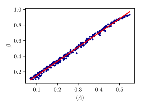
Figure 11: The level repulsion exponent $\beta$ as a function of the entropy localization measure $\left<A\right>$ for variety of stadia of different shapes $\varepsilon$ and energies $E=k^{2}$, as defined in the text.

This relation $\beta(\left<A\right>)$ is very similar to the case of the quantum kicked rotator Izrailev (1990); Manos and Robnik (2013); Batistić et al. (2013). In both cases the scattering of points around the mean linear behaviour is significant, and it is related to the fact that the localization measure $A$ of eigenstates has some distribution $P(A)$, as observed and discussed in Ref. Manos and Robnik (2015) for the quantum kicked rotator, and discussed for the stadium billiard in the previous section IV.

There is still a great lack in theoretical understanding of the physical origin of this phenomenon, even in the case of (the long standing research on) the quantum kicked rotator, except for the intuitive idea, that energy spectral properties should be only a function of the degree of localization, because the localization gradually decouples the energy eigenstates and levels, switching the linear level repulsion $\beta=1$ (extendedness) to a power law level repulsion with exponent $\beta<1$ (localization). The full physical explanation is open for the future.

As shown in Batistić et al. (2018) and in Fig. 12 the functional dependence of $\beta(\alpha)$ is always the rational function

$$\beta=\beta_{\infty}\frac{s\alpha}{1+s\alpha}.$$ (24)

only the coefficient $s$ depends on the definition of $N_{T}$ and $\alpha$. For the exponential law we found $\beta_{\infty}=0.98$ and $s=0.20$.

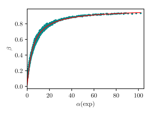
Figure 12: The level repulsion exponent $\beta$ as a function of $\alpha$ fitted by the function (24), based on $N_{T}$ from the exponential diffusion law. $\beta_{\infty}=0.98$ and $s=0.20$.

Finally, we look at the dependence of $\sigma$ on $\beta$, shown in Fig. 13. It should be noted that dependence of $\sigma$ on $\left<A\right>$ is nearly the same, because $\beta$ and $\left<A\right>$ are linearly related, as demonstrated in Fig. 11.

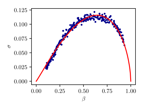
Figure 13: The standard deviation $\sigma$ as a function of the level repulsion exponent $\beta$ for variety of stadia of different shapes $\varepsilon$ and energies $E=k^{2}$, as defined in the text. The best fitting curve for this empirical function is from Eq. (18), with the parameter values $C=0.345$, $a=1.07$ and $b=0.60$. $C$ is determined by fitting, not by normalization, as $\sigma(\beta)$ is a function, not a distribution.

It is surprising that also here the best fit of the function is found by choosing the beta distribution (18) with the parameters $a=1.07$, $b=0.60$, $C=0.08$ and $\beta$ is on the interval $[0,1]$.

VI Conclusions and discussion

We have shown that in the stadium billiard of Bunimovich Bunimovich (1979) the localization measure $A$, based on the information entropy, of eigenstates as described by the Poincaré - Husimi functions, has a distribution $P(A)$ very well described by the beta distribution. We have also looked at the mean $\left<A\right>$ and the standard deviation $\sigma$ as functions of the major control parameter $\alpha$, the ratio of the Heisenberg time and the classical transport (diffusion) time. We have also shown that the normalized inverse participation ratio is equivalent to $A$.

The spectral level repulsion exponent $\beta$ of the localized eigenstates is functionally related to $\left<A\right>$ Batistić et al. (2018). Moreover, the dependence is linear, as in the quantum kicked rotator, but somewhat different from the case of a mixed type billiard studied recently by Batistić and Robnik Batistić and Robnik (2013a, b), where the high-lying localized chaotic eigenstates have been analyzed after the separation of regular and chaotic eigenstates.

$\beta$ is empirically a rational function of the major control parameter $\alpha$. The definition of the classical transport time is to some extent arbitrary, but we have shown in Batistić et al. (2018) that the various definitions do not change the shape of the dependence on $\varepsilon$, but instead affect only the prefactor. As a consequence of that the dependence is empirically (by best fit) always a rational function. The transition from complete localization $\beta=0$ to the complete extendedness (delocalization) $\beta\approx 1$ takes place very smoothly, over about almost two decades of the parameter $\alpha$.

Thus we have again demonstrated by numerical calculation that the fractional power law level repulsion with the exponent $\beta\in[0,1]$ is manifested in localized chaotic eigenstates. The dependence $\beta(\left<A\right>)$ has some scatter due to the fact that $A$ has above mentioned distribution $P(A)$ with nonzero $\sigma$.

Our empirical findings call for theoretical explanation, which is a long standing open problem even for the main paradigm of quantum chaos, the quantum kicked rotator studied extensively over the decades Izrailev (1990).

Further theoretical work is in progress. Beyond the billiard systems, there are many important applications in various physical systems, like e.g. in hydrogen atom in strong magnetic field Robnik (1981, 1982); Hasegawa et al. (1989); Wintgen and Friedrich (1989); Ruder et al. (1994), which is a paradigm of stationary quantum chaos, or e.g. in microwave resonators, the experiments introduced by Stöckmann around 1990 and intensely further developed since then Stöckmann (1999).

VII Acknowledgement

This work was supported by the Slovenian Research Agency (ARRS) under the grant J1-9112.

References

- Stöckmann (1999) H.-J. Stöckmann, Quantum Chaos - An Introduction (Cambridge: Cambridge University Press, 1999).
- Haake (2001) F. Haake, Quantum Signatures of Chaos (Berlin: Springer, 2001).
- Robnik (2016) M. Robnik, Eur. Phys. J. Special Topics 225, 959 (2016).
- Casati et al. (1979) G. Casati, B. V. Chirikov, F. M. Izrailev, and J. Ford, Lecture Notes in Physics 93, 334 (1979).
- Chirikov et al. (1981) B. V. Chirikov, F. M. Izrailev, and D. L. Shepelyansky, Sov. Sci. Rev. C 2, 209 (1981).
- Chirikov et al. (1988) B. V. Chirikov, F. M. Izrailev, and D. L. Shepelyansky, Physica D 33, 77 (1988).
- Izrailev (1990) F. M. Izrailev, Phys. Rep. 196, 299 (1990).
- Izrailev (1988) F. M. Izrailev, Phys. Lett. A 134, 13 (1988).
- Izrailev (1989) F. M. Izrailev, J. Phys. A: Math. Gen. 22, 865 (1989).
- Fishman et al. (1982) S. Fishman, D. R. Grempel, and R. E. Prange, Phys. Rev. Lett. 49, 509 (1982).
- Prosen (2000) T. Prosen, in Proc. of the Int. School in Phys. ”Enrico Fermi”, Course CXLIII, Eds. G. Casati and U. Smilansky (Amsterdam: IOS Press, 2000).
- Batistić and Robnik (2013a) B. Batistić and M. Robnik, Phys. Rev. E 88, 052913 (2013a).
- Robnik (1983) M. Robnik, J. Phys. A: Math. Gen. 16, 3971 (1983).
- Robnik (1984) M. Robnik, J. Phys. A: Math. Gen. 17, 1049 (1984).
- Batistić and Robnik (2013b) B. Batistić and M. Robnik, J. Phys. A: Math. Theor. 46, 315102 (2013b).
- Batistić et al. (2018) B. Batistić, Č. Lozej, and M. Robnik, Nonlinear Phenomena in Complex Systems (Minsk) 21, 225 (2018).
- Bunimovich (1979) L. Bunimovich, Commun. Math. Phys. 65, 295 (1979).
- Borgonovi et al. (1996) F. Borgonovi, G. Casati, and B. Li, Phys. Rev. Lett. 77, 4744 (1996).
- Č. Lozej and Robnik (2018) Č. Lozej and M. Robnik, Phys. Rev. E 97, 012206 (2018).
- Mehta (1991) M. L. Mehta, Random Matrices (Boston: Academic Press, 1991).
- Guhr et al. (1998) T. Guhr, A. Müller-Groeling, and H. Weidenmüller, Phys. Rep. 299, 4 (1998).
- Robnik (1998) M. Robnik, Nonl. Phen. in Compl. Syst. (Minsk) 1, 1 (1998).
- Percival (1973) I. C. Percival, J. Phys B: At. Mol. Phys. 6, L229 (1973).
- Berry and Robnik (1984) M. V. Berry and M. Robnik, J. Phys. A: Math. Gen. 17, 2413 (1984).
- Batistić and Robnik (2010) B. Batistić and M. Robnik, J. Phys. A: Math. Theor. 43, 215101 (2010).
- Casati et al. (1980) G. Casati, F. Valz-Gris, and I. Guarneri, Lett. Nuovo Cimento 28, 279 (1980).
- Bohigas et al. (1984) O. Bohigas, M. J. Giannoni, and C. Schmit, Phys. Rev. Lett. 52, 1 (1984).
- Sieber and Richter (2001) M. Sieber and K. Richter, Phys. Scr. T90, 128 (2001).
- Müller et al. (2004) S. Müller, S. Heusler, P. Braun, F. Haake, and A. Altland, Phys. Rev. Lett. 93, 014103 (2004).
- Heusler et al. (2004) S. Heusler, S. Müller, P. Braun, and F. Haake, J. Phys.A: Math. Gen. 37, L31 (2004).
- Müller et al. (2005) S. Müller, S. Heusler, P. Braun, F. Haake, and A. Altland, Phys. Rev. E 72, 046207 (2005).
- Müller et al. (2009) S. Müller, S. Heusler, A. Altland, P. Braun, and F. Haake, New J. of Phys. 11, 103025 (2009).
- Gutzwiller (1980) M. C. Gutzwiller, Phys. Rev. Lett. 45, 150 (1980).
- Berry (1985) M. V. Berry, Proc. Roy. Soc. Lond. A 400, 229 (1985).
- Brody (1973) T. A. Brody, Lett. Nuovo Cimento 7, 482 (1973).
- Brody et al. (1981) T. A. Brody, J. Flores, J. B. French, P. A. Mello, A. Pandey, and S. S. M. Wong, Rev. Mod. Phys. 53, 385 (1981).
- Manos and Robnik (2013) T. Manos and M. Robnik, Phys. Rev. E 87, 062905 (2013).
- Batistić et al. (2013) B. Batistić, T. Manos, and M. Robnik, EPL 102, 50008 (2013).
- Manos and Robnik (2015) T. Manos and M. Robnik, Phys. Rev. E 91, 042904 (2015).
- Berry (1981) M. V. Berry, Eur. J. Phys. 2, 91 (1981).
- Wigner (1932) E. Wigner, Phys. Rev. 40, 749 (1932).
- Husimi (1940) K. Husimi, Proc. Phys. Math. Soc. Jpn. 22, 264 (1940).
- Tualle and Voros (1995) J. Tualle and A. Voros, Chaos Solitons Fractals 5, 1085 (1995).
- Bäcker et al. (2004) A. Bäcker, S. Fürstberger, and R. Schubert, Phys. Rev. E 70, 036204 (2004).
- Vergini and Saraceno (1995) E. Vergini and M. Saraceno, Phys. Rev. E 52, 2204 (1995).
- Shnirelman (1974) B. Shnirelman, Uspekhi Matem. Nauk 29, 181 (1974).
- Heller (1984) E. J. Heller, Phys. Rev. Lett. 53, 1515 (1984).
- Robnik (1981) M. Robnik, J. Phys. A: Math. Gen. 14, 3195 (1981).
- Robnik (1982) M. Robnik, J. Phys. Colloque C2 43, 29 (1982).
- Hasegawa et al. (1989) H. Hasegawa, M. Robnik, and G. Wunner, Prog. Theor. Phys. Suppl. (Kyoto) 98, 198 (1989).
- Wintgen and Friedrich (1989) D. Wintgen and H. Friedrich, Phys. Rep. 183, 38 (1989).
- Ruder et al. (1994) H. Ruder, G. Wunner, H. Herold, and F. Geyer, Atoms in Strong Magnetic Fields (Heidelberg: Springer, 1994).