A Rational Inattention Theory of Echo Chamber

Abstract

We develop a rational inattention theory of echo chamber, whereby players gather information about an uncertain state by allocating limited attention capacities across biased primary sources and other players. The resulting Poisson attention network transmits information from the primary source to a player either directly, or indirectly through the other players. Rational inattention generates heterogeneous demands for information among players who are biased toward different decisions. In an echo chamber equilibrium, each player restricts attention to his own-biased source and like-minded friends, as the latter attend to the same primary source as his, and so could serve as secondary sources in case the information transmission from the primary source to him is disrupted. We provide sufficient conditions that give rise to echo chamber equilibria, characterize the attention networks inside echo chambers, and use our results to inform the design and regulation of information platforms.

Keywords: rational inattention, echo chamber, information platform design and regulation

JEL codes: D83, D85

1 Introduction

The Cambridge English Dictionary defines echo chambers as “environments in which people encounter mostly beliefs or opinions that coincide with their own, so that their existing views are reinforced and alternative ideas are seldom considered.” Examples that fit this description have recently flourished on the Internet and social media; their economic and social consequences have been the subject of heated debate in the academia and popular press (Bakshy et al., 2015; Del Vicario et al., 2016; Barberá, 2020; Cossard et al., 2020). Most ongoing discussions of echo chambers focus on their behavioral roots (Levy and Razin, 2019). This paper develops a theory of echo chamber based on the premise of rational inattention.

We use the term rational inattention (RI) to refer to the rational and flexible allocation of limited attention capacities across information sources. Such a premise has become increasingly relevant in today’s digital age, as people are inundated with information on the one hand, but can selectively choose which information sources to visit using personalization technologies on the other hand. Since Sunstein (2007) and Pariser (2011), it has been long suspected that RI may engender a selective exposure to content and a formation of homogeneous opinion clusters. The current paper formalizes this idea by prescribing conducive conditions to echo chamber formation among rationally inattentive decision makers. We also characterize the attention networks inside echo chambers, and use our results to inform the design and regulation of information platforms.

We embed the analysis in a simple model of decision making under uncertainty. To illustrate our framework, consider new parents who are about to feed their babies with solid food. Each parent must choose between a traditional approach denoted by $A$ (e.g., spoon feeding), and a new approach denoted by $B$ (e.g, baby-led weaning). Which approach is better for baby development is modeled as a random state that is either $A$ or $B$ with equal probability. A parent earns the highest level of utility from choosing the best approach for baby development. Otherwise he incurs a loss of a varying magnitude, depending on whether the adopted approach matches his own preference or not (e.g., baby-led weaning may be more preferred because it is easy to prepare). Given the prior belief about the state, the default decision is to adopt the parent’s preferred approach.

To gather information about the state, a parent pays attention to information sources. We distinguish between primary sources and secondary sources. The former generate original data about the state. In our leading example, they constitute scientific experiments published in pediatric journals. As in Che and Mierendorff (2019), we model two biased primary sources called $A$-revealing and $B$-revealing. The $\omega$-revealing source, $\omega\in\{A,B\}$, is an experiment designed to reject the null hypothesis that the state is $\omega^{\prime}\neq\omega$. It works by revealing that the state is $\omega$ when it is and keeping silent otherwise. Secondary sources are our innovation. In our leading example, they constitute parents who consume and pass along primary source content to other parents via online support groups. A parent is endowed with a limited amount of attention, or bandwidth, that can be allocated across the various sources in a flexible manner. A feasible attention strategy specifies a nonnegative amount of attention that the parent pays to each source, subject to the constraint that the total amount of paid attention must not exceed his bandwidth.

The subject of our study is the Poisson attention network generated by parents’ attention strategies. After these strategies are specified, the state $\omega$ is realized, and messages thereof are circulated in the society for two rounds. In the first round, the $\omega$-revealing primary source disseminates a message “$\omega$” to parents. The message reaches each parent independently with a Poisson probability that increases with the amount of attention the latter pays to the primary source. In the second round, those parents who received a message in the previous round pass it along to the other parents using Poisson technologies. The probability of a successful information transmission between a parent pair increases with the sender’s visibility as a secondary source (i.e., the rate of his Poisson technology), as well as the amount of attention the recipient pays to the sender. After that, parents update beliefs and make final decisions. We characterize the attention networks that can arise in equilibrium.

Our notion of echo chamber has two defining features. The first is a selective exposure to content and a formation of homogeneous clusters. Specifically, we define a parent’s own-biased source as the primary source that favors his default decision as the null hypothesis, and call two parents like-minded friends if they share the same default decision. We say that echo chambers arise in an equilibrium if all parents restrict attention to their own-biased sources and like-minded friends on the equilibrium path. The second feature is a belief polarization coupled with an occasional, drastic, belief reversal. It is easy to see that after playing an echo chamber equilibrium, each parent receives no message from any source most of the time and updates the belief in favor of his default decision in that event. With a small complementary probability, the opposite happens, and the parent feels strongly about abandoning his default approach. As will later be discussed in Footnote 7, both features of echo chambers have suggestive empirical supports.

Our main results exploit the trade-off between primary and secondary sources. The first result prescribes sufficient conditions for the rise of echo chamber equilibria. Since a parent can always make his default decision without paying attention, paying attention is only useful if it sometimes convinces him to act differently. When attention is limited, the parent should, intuitively, focus on his own-biased source, as the information generated by the latter disapproves of his default decision. Likewise, he should attend only to his like-minded friends but no one else, as the former share the same primary source with him, and so could serve as secondary sources in case the information transmission from the own-biased source to him is disrupted. A caveat to this argument is the potential strategic gain from switching sides: when many other parents are gathering the opposite kind of information, a parent may want to follow suit so as to gain access to many secondary sources. Nevertheless, such a gain is shown to be limited when parents are sufficiently biased, when there are many people to attend to, and when attention is scarce. These conditions closely mirror the world we are living in, as technology advances have turned the entire globe into a village and inundated people with more information than anyone can process in a lifetime. These trends are conducive to echo chamber formation, especially when people are sufficiently biased to begin with.

Our second result characterizes the equilibrium attention network inside an echo chamber. We define a parent’s informedness (as a secondary source) as the amount of attention that he pays to the primary source, while capturing his influence on public opinion by the amount of attention he attracts from his friends. We find that the game among like-minded friends exhibits strategic substitutability, as raising one’s informedness attracts more attention of his friends away from the primary source to him. Based on this finding, together with other basic model properties, we develop a method for investigating the comparative statics of equilibrium attention networks. Our findings are threefold.

First, increasing a parent’s bandwidth promotes his informedness and influence while diminishing that of any other parent. This equilibrium mechanism is shown to magnify even a small difference between parents’ bandwidths into a very uneven distribution of opinions, whereby some parents act as opinion leaders, whereas others act as opinion followers. An important feature of today’s news landscape is that while most Americans are interested in many topics such as science, economy, and politics, only a minority of them are serious news consumers, due to the distractions that come from overabundant entertainment opportunities (Funk et al., 2017). The attention gap between the majority and minority may generate patterns such as the law of the few and fat-tailed opinion distributions, whose presence in the social media sphere has recently been detected by Lu et al. (2014) and Del Vicario et al. (2016).

In contrast, varying players’ visibility has, in general, ambiguous effects on the equilibrium attention network. We postpone the discussion of intuition till Section 4.1, and point out here the potential of this result in informing the design and regulation of information platforms: to counter the rising threat of misinformation and fake news, many social media platforms have recently taken measures to modulate users’ visibility. We caution that such interventions may entail unintended consequences unless they are calibrated exactly according to the underlying environment.

Finally, we evaluate the usefulness of anti-polarization platforms such as Allsides.com, which expose users to balanced viewpoints from both sides. We model such platforms as a mega source that obtains from merging the biased primary sources of the baseline model together. On the one hand, the use of mega source dissolves echo chambers by forcing different types of parents to attend to each other as secondary sources. Yet increasing access to secondary sources discourages information acquisition from primary sources. The resulting free-riding problem can render the overall welfare impact ambiguous, as shown by our comparative statics regarding players’ population size.

In Section 6, we study a political economy application of our model, whereby partisan voters vote instrumentally between a Democratic candidate and Republican candidate based on their qualities. Information thereof is generated by biased media outlets, whose reporting sends either an “ideological message” that conforms with the outlet’s ideological bias, or a “newsworthy message” that goes against its bias. As a newsworthy message traverses through voters’ attention network, it gets lost and is replaced with an ideological message probabilistically. Intuitively, a reader with a gut feeling that the NYTimes’ reporting is pro-liberal may grasp its pro-conservative nature after parsing the content, but such a success cannot be guaranteed, due to the attention bottleneck on the reader’s side. Our results shed light on when and why echo chambers may arise in this environment, how voters’ beliefs and behaviors are distributed after playing an echo chamber equilibrium, and why various policy responses to current events may have limited or unintended consequences.

1.1 Related literature

Rational inattention.

A central question addressed by the RI literature concerns the flexible acquisition of information about a payoff-relevant state by a single decision maker (see Maćkowiak et al. 2023 for a survey). For that purpose, it is useful to model information acquisition strategies as signal structures that map fundamental states to lotteries over terminal actions. This compact representation, however, abstracts away from how decision makers learn from multiple information sources, especially when the latter are themselves the players of a strategic game. In games with strategic complementarities, Hellwig and Veldkamp (2009), Denti (2023, 2017), and Hébert and La’O (2023) demonstrate the usefulness of attending to the endogenous signals gleaned by other players, as the latter affect other players’ decisions to coordinate and, hence, are payoff relevant. This is not the case in our model, where one’s utility depends only on his action and a payoff-relevant state. In equilibrium, a player is attended by others because he has a better information dissemination technology than primary sources’. Evidence for the last assumption is discussed in Sections 2.2 and 6, when we present examples and applications of our model.

Filtering bias is an important form of media/political bias (Gentzkow et al., 2015). The idea behind it — namely even a rational decision maker can exhibit a preference/demand for biased information when constrained by information processing capacities — dates back to Calvert (1985), and is later expanded on by Suen (2004), Che and Mierendorff (2019), Zhong (2022), and Hu et al. (2023) among others, in single agent decision making problems. We examine the validity of this idea in a strategic setting, where one’s choice of attention strategy depends not only on his own preference, but also on the attention strategies of other players. Our focus on the allocation of attention between primary and secondary sources in a static game differs from that of Che and Mierendorff (2019). The latter study a dynamic information acquisition problem faced by a single decision maker, who repeatedly allocates a limited amount of attention between biased, Poisson, signals. These authors observe, like we do, that the decision maker should focus exclusively on his own-biased source in a static environment. Their main research question addresses how this baseline prediction is altered by the dynamics of information acquisition.

We are not the first to study Poisson attention networks. Dessein et al. (2016) first analyze the efficient Poisson attention network among nonstrategic members of an organization with adaptation and coordination motives. We focus on the equilibrium attention network among strategic players, although we do solve for the efficient attention network of a symmetric society as an extension. Our players’ objective functions also differ from that of Dessein et al. (2016).

Social network.

The literature on social network is vast. Here we focus on background reviews, as well as immediate predecessors to our work. Additional papers will be discussed as the paper proceeds.

Inside an echo chamber, our game combines (i) the strategic formation of an information sharing network, with (ii) a network game in which players’ investments (in informedness) exhibit strategic substitutability. Studies of non-cooperative network formation games without endogenous investments were pioneered by Jackson and Wolinsky (1996) and Bala and Goyal (2000), and have recently been advanced by Calvó-Armengol et al. (2015) and Herskovic and Ramos (2020) among others. The last two papers bestow players with exogenous signals and focus on the formation of information sharing networks, whereas signals are endogenous in our model. Existing network-formation models work mainly with discrete links. Links are divisible here, as well as in Bloch and Dutta (2009), Baumann (2021), and Elliott et al. (2022), among others.

A vast literature studies how to play games with strategic substitutes on a fixed network (see Jackson and Zenou 2015 for a survey). Most methodological contributions to this literature concern the uniqueness and stability of the equilibrium, with many early contributions assuming linear best response functions or a symmetric influence matrix between players (see, e.g., Parise and Ozdaglar 2019 and Bramoullé et al. 2014, respectively). We develop a toolkit for investigating equilibrium comparative statics under different assumptions from the aforementioned.

A few recent papers study hybrid games that are akin to ours (see Sadler and Golub 2021 for a recent survey). Galeotti and Goyal (2010) also study a model of information acquisition, followed by information sharing. Designed to address a different host of questions, their model assumes homogeneous players and quantitative information acquisition (i.e., how much information is acquired rather than what kind of information is acquired), and so cannot be immediately applied to the study of echo chamber formation among heterogeneous players. Nor does it inform the consequences of augmenting players’ visibility or promoting cross-cutting exposures — topics that are central to our comparative statics exercise. Its main prediction: the law of the few, is obtained under a different information technology and based on different reasoning from ours.

Rational theories of echo chamber.

A small but growing literature investigates the rational origins of echo chambers. The closest work to ours: Baccara and Yariv (2013) (BY), studies a model of group formation, followed by the production and sharing of information among group members. The main differences between BY and the current work are threefold. First, BY models information as a local public good that is automatically shared among group members. Here, the decision to acquire secondhand information from other players is private and strategic. Second, BY codes players’ preferences for information in their utility functions. Here, such a preference arises endogenously from limited attention. Third, BY’s reasoning exploits the sorting of people with similar preferences into groups of limited sizes. We impose no restriction on the sizes of echo chambers and do not invoke the sorting logic.

Other rational theories of echo chamber fall broadly into two categories: (i) strategic communication or information disclosure between players with conflicting objectives (Galeotti et al., 2013; Jann and Schottmüller, 2021; Innocenti, 2021; Meng, 2021); (ii) learning from sources with unknown biases (Sethi and Yildiz, 2016; Williams, 2023). Neither consideration is present in our model, where sources are nonstrategic, and their biases are commonly known.

2 Baseline model

In this section, we describe the model setup, followed by model discussions and then an illustrative example.

2.1 Setup

A finite set $\mathcal{I}$ of players faces two equally likely states $A$ and $B$. Each player $i\in\mathcal{I}$ has a type $t_{i}\in\{A,B\}$ (also called his default decision), and makes a terminal decision $d_{i}\in\{A,B\}$. His utility is normalized to zero if the decision matches the true state. In case the two objects differ, the player incurs a loss of magnitude $\beta_{i}\in(0,1)$ from making the default decision. Otherwise the loss has magnitude 1. Formally,

$$u_{i}(d_{i},\omega)=\begin{cases}0&\text{ if }d_{i}=\omega,\\ -\beta_{i}&\text{ if }d_{i}\neq\omega\text{ and }d_{i}=t_{i},\\ -1&\text{ if }d_{i}\neq\omega\text{ and }d_{i}\neq t_{i}.\end{cases}$$

The assumption $\beta_{i}\in(0,1)$ implies that the default decision is the most preferred given the prior belief about the state distribution. Such a preference becomes stronger as we reduce $\beta_{i}$, which is hereinafter referred to as the player’s horizontal preference parameter. Let $\mathcal{A}$ and $\mathcal{B}$ denote the sets of type $A$ players and type $B$ players, respectively. Assume throughout that $|\mathcal{A}|,|\mathcal{B}|\geq 2$.

There are two primary sources called $A$-revealing and $B$-revealing. In state $\omega\in\{A,B\}$, the $\omega$-revealing primary source announces a message “$\omega$,” whereas the other primary source is silent. The message “$\omega$” fully reveals that the state is $\omega$, since any player would assign probability one to the state being $\omega$ given this message. To gather information about the state, a player can pay attention to the primary sources, i.e., spend valuable time on them. In addition, he can pay attention to the other players as potential secondary sources. For each player $i\in\mathcal{I}$, $\mathcal{C}_{i}=\{\text{A-revealing},\text{B-revealing}\}\cup\mathcal{I}-\{i\}$ denotes the set of the sources he can pay attention to. An attention strategy $x_{i}=(x_{i}^{c})_{c\in\mathcal{C}_{i}}$ specifies a nonnegative amount $x_{i}^{c}\geq 0$ of attention that the player pays to each source $c\in\mathcal{C}_{i}$; it is feasible if it satisfies the player’s bandwidth constraint $\sum_{i\in\mathcal{C}_{i}}x_{i}^{c}\leq\tau_{i}$, which stipulates that the total amount of paid attention must not exceed his bandwidth $\tau_{i}>0$. Let $\mathcal{X}_{i}$ denote the set of feasible attention strategies for player $i$. To capture the flexibility of attention allocation, we allow for the adoption of any strategy in $\mathcal{X}_{i}$.

After players specify their attention strategies, the state $\omega\in\{A,B\}$ is realized, and messages thereof are circulated in the society for two rounds.

• In the first round, the $\omega$-revealing primary source disseminates “$\omega$” to players using a Poisson technology with rate $1$. The message reaches each player $i\in\mathcal{I}$ independently with probability $1-\exp(-x_{i}^{\omega\emph{\text{-revealing}}})$, which increases with the amount $x_{i}^{\omega\emph{\text{-revealing}}}$ of attention that player $i$ pays to the primary source and is strictly bounded above by one. The last property captures the scarcity of attention relative to the available information in the world.

• In the second round, each player $i$ who received a message in the first round passes it along to the others using a Poisson technology with rate $\lambda_{i}>0$. The message reaches each player $j\in\mathcal{I}-\{i\}$ independently with probability $1-\exp(-\lambda_{i}x_{j}^{i})$, which increases with the amount $x_{j}^{i}$ of attention player $j$ pays to player $i$. The parameter $\lambda_{i}$ captures player $i$’s visibility as a secondary source, and is hereinafter referred to as his visibility parameter.

After two rounds of information transmission, players update beliefs about the state and make final decisions. The game sequence is summarized as follows.

1. Players choose attention strategies.

2. The state $\omega$ is realized.

3. 1. The $\omega$-revealing source disseminates message “$\omega$” to players.

   2. Those players who received messages in Stage 3(a) pass them along to the other players.

4. Players update beliefs and make final decisions.

The solution concept is pure strategy perfect Bayesian equilibrium (PSPBE), or equilibrium for short.

Model discussions.

Throughout, we work with Poisson attention technologies to gain tractability. Other simplifying assumptions include: the decision problem is binary, messages are fully revealing of the true state, and information transmission between players lasts for one round. We relax these assumptions and examine its impact on our predictions toward the end of Section 3.3.

The assumption of nonstrategic information transmission is without loss of generality: since players care only about their own decisions and the true state, but not about any other player or aggregate outcome, they have no incentive to distort communication even if it is a possibility.

2.2 Illustrative example

The illustrative example presented below formalizes the story told in the introduction.

Example 1.

A group of new parents is about to feed their babies with solid foods. There are two approaches: $A=$ traditional spoon-feeding, and $B=$ new baby-led weaning. Under the traditional approach, parents spoon-feed babies first with purée food and then with different stages of baby food until babies are strong enough to eat on their own. The new approach skips traditional baby food and puts babies in charge of their mealtime. Babies are given chucks of suitable food such as banana or bread, and they hold the food in their hands and feed themselves.

Which approach is better for baby development is an open question. For example, a possible downside of baby-led weaning is that babies tend to eat less and choke more in the first few months. Whether this issue has any long-term health consequence and how it should be weighed against the upside of the new approach (e.g., practice motor skills earlier and build healthy eating habits), are topics of active research. The uncertainty surrounding the truth is captured by the random state $\omega\in\{A,B\}$.

A parent’s preference has two dimensions. The vertical dimension varies, depending on which approach is better for baby development. The horizontal dimension, as parameterized by $\beta_{i}$, captures the parent’s own preference: some parents prefer the traditional approach because it is less messy; others prefer the new approach because it skips purée foods and so is easier to prepare. A parent earns the highest level of utility from adopting the best approach for baby development. Otherwise he incurs a loss of a varying magnitude, depending on whether the adopted approach matches his own preference or not.

Information about the uncertain state is generated by two kinds of scientific experiments: those designed to reject the traditional approach, and those designed to reject the new approach. These experiments constitute the primary sources in our model. Parents can read directly about the experiments published in scientific journals. Alternatively, they can learn from the secondhand opinions shared by other parents on online support groups — Academic Moms, BabyCenter, to name a few.

Parents may differ in the amount of available time $\tau_{i}$s for information gathering, depending on the nature of their work, the length of parental leave, etc. They may also differ in their visibility $\lambda_{i}$s as secondary sources. For example, parents who are well-educated and good at explaining science to layman attract many followers on online platforms; the decision on whether to post a video on Youtube depends on how keen one is on helping others, as well as how tech-savvy he is. $\hfill\diamondsuit$

3 Analysis

This section conducts equilibrium analysis. We begin by formalizing players’ problems in Section 3.1, and presenting key concepts in Section 3.2. These are followed by the statements of main theorems and their discussions in Sections 3.3 and 3.4.

3.1 Player’s problem

Under any joint attention strategy profile $x\in\mathcal{X}\coloneqq\times_{i\in\mathcal{I}}\mathcal{X}_{i}$, the transmission of information from the $\omega$-revealing source to player $i$ is disrupted with probability

$$\delta_{i}^{\omega\emph{-revealing}}\coloneqq\exp(-x_{i}^{\omega\emph{-revealing}}),$$

and the transmission of information from any player $j\in\mathcal{I}-\{i\}$ to him is disrupted with probability

$$\delta_{i}^{j}\coloneqq\exp(-\lambda_{j}x_{i}^{j}).$$

Let $\mathcal{U}_{i}$ denote the event in which the above attention channels are all disrupted, and so player $i$ remains uninformed of the state at Stage 4 of the game (hereinafter, the decision making stage). The probability of $\mathcal{U}_{i}$ in state $\omega$ equals

$$\mathbb{P}_{x}\left(\mathcal{U}_{i}\mid\omega\right)\coloneqq\delta_{i}^{\omega\emph{-revealing}}\prod_{j\in\mathcal{I}-\left\{i\right\}}(\delta_{j}^{\omega\emph{-revealing}}+(1-\delta_{j}^{\omega\emph{-revealing}})\delta_{i}^{j}).$$

At the decision making stage, either player $i$ learns the true state and earns zero utility; or event $\mathcal{U}_{i}$ happens, in which case even optimal decision making incurs a loss probabilistically. The expected utility generated by the optimal decision rule equals

$$\max\{-\frac{\beta_{i}}{2}\mathbb{P}_{x}\left(\mathcal{U}_{i}\mid\omega\neq t_{i}\right),-\frac{1}{2}\mathbb{P}_{x}\left(\mathcal{U}_{i}\mid\omega=t_{i}\right)\},$$

where the first and second terms in the big bracket represent the expected losses incurred from making the default decision and the other decision in event $\mathcal{U}_{i}$, respectively. At Stage 1 of the game (hereinafter the attention paying stage), the player chooses an attention strategy $x_{i}\in\mathcal{X}_{i}$ to maximize the last expression, taking the attention strategies $x_{-i}\in\times_{j\in\mathcal{I}-\{i\}}\mathcal{X}_{j}$ of other players as given.

3.2 Key concepts

We first define the biases of primary sources in a manner that is standard in the literature on filtering bias (as reviewed in Section 1.1).

Definition 1.

A primary source is biased toward decision $d\in\{A,B\}$ (or simply $d$-biased) if receiving no message from it increases one’s belief that the state favors decision $d$. A player’s own-biased source is the primary source that is biased toward his default decision.

In the leading example, the $A$-revealing source is an experiment designed to reject approach $B$. It does so through generating $A$-revealing evidence, absent of which approach $B$ becomes more favorable, hence the name “$B$-biased.” A parent’s own-biased source favors his preferred approach as the null hypothesis. In what follows, we will denote the $A$-revealing (resp. $B$-revealing) source by $b$ (resp. $a$). Type $A$ (resp. $B$) players’ own-biased source is $a$ (resp. $b$).

Next is the notion of like-minded friends.

Definition 2.

Two players are like-minded friends if they share the same default decision (and, hence, the same own-biased source).

Next is the key definition of echo chamber equilibrium.

Definition 3.

An equilibrium is an echo chamber equilibrium if each player attends only to his own-biased source and like-minded friends on the equilibrium path.

An echo chamber equilibrium has two noteworthy features. The first is a selective exposure to content and a formation of homogeneous clusters. The second is a belief polarization coupled with an occasional, drastic, belief reversal. After playing an echo chamber equilibrium, each player receives no message from any source most of the time and updates the belief in favor of his default decision in that event. With a small complementary probability, the opposite happens, and the player feels strongly about abandoning his default decision. As discussed in Footnote 7 of the introduction, both features of echo chambers have suggestive empirical support.

While many of our results hold in general environments, some speak only to the symmetric equilibria in symmetric environments.

Definition 4.

A society is symmetric if both types of players have the same population size $N$ and the same characteristic profile $(\beta,\lambda,\tau)$. An equilibrium is symmetric if the equilibrium strategy depends only on the amount of attention that a typical player pays to his own-biased source, the other primary source, each like-minded friend of his, and any other player, respectively.

We finally introduce two useful functions. Their main properties, as listed below, will soon be invoked when we reason about players’ best response functions.

Definition 5.

For each $\lambda\geq 0$, define

$$\phi\left(\lambda\right)\coloneqq\begin{cases}\log(\frac{\lambda}{\lambda-1})&\text{if }\lambda>1,\\ +\infty&\text{if }\lambda\in[0,1].\end{cases}$$

For each $\lambda>1$ and $x\in[\phi\left(\lambda\right),+\infty)$, define

$$h\left(x;\lambda\right)\coloneqq\frac{1}{\lambda}\log\left[\left(\lambda-1\right)\left(\exp\left(x\right)-1\right)\right].$$

Observation 1.

$\phi^{\prime}(\lambda)<0$ on $\left(1,+\infty\right)$ and $\lim_{\lambda\downarrow 1}\phi(\lambda)=+\infty$. For each $\lambda>1$, $h(\phi(\lambda),\lambda)=0$ and $h_{x}\left(x;\lambda\right)\in\left(0,1\right)$ on $(\phi\left(\lambda\right),+\infty)$.

3.3 Echo chamber formation

Our first theorem provides sufficient conditions for the rise of echo chamber equilibria.

Theorem 1.

(i) Fix any population sizes $|\mathcal{A}|,|\mathcal{B}|\geq 2$ and characteristic profile $\left(\lambda_{i},\tau_{i}\right)_{i\in\mathcal{A}\cup\mathcal{B}}\in\mathbb{R}_{++}^{2(|\mathcal{A}|+|\mathcal{B}|)}$. There exists $\underline{\beta}\in\left(0,1\right)$ such that when $\beta_{i}\in(0,\underline{\beta})$ for all $i\in\mathcal{I}$, every equilibrium of the game is an echo chamber equilibrium. (ii) Consider symmetric societies parameterized by $(N,\beta,\lambda,\tau)$, where $N\geq 2$, $\beta\in(0,1)$, and $\lambda,\tau>0$.

1. For any $\beta$, $\lambda$, and $\tau$ as above, there exists $\underline{N}\geq 2$ such that for any $N\geq\underline{N}$, the unique symmetric equilibrium of the game is an echo chamber equilibrium.

2. For any $\beta$, $\lambda$, and $N$ as above, there exists $\underline{\tau}>0$ such that for any $\tau\leq\underline{\tau}$, the unique symmetric equilibrium of the game is an echo chamber equilibrium.

The conditions prescribed Theorem 1 closely mirror the world we are living in. As more and more people turn to the Internet and social media where the amount of available information is vastly greater than any individual can process in a lifetime, it is reasonable to model bandwidth $\tau_{i}$s as finite, if not small, numbers. Meanwhile, the use of automated systems has enabled virtual connections between people who seldom meet each other in reality, hence our focus on the case of a large population size $N$ is justified, and the assumption of flexible attention allocation across information sources seems legitimate. Theorem 1 shows that these conditions are conducive to echo chamber formation, especially when people are sufficiently biased, i.e., $\beta_{i}$s are small.

Proof ideas.

We outline the proof ideas behind Theorem 1, in two steps.

Step 1: basic intuition. Consider first a benchmark case in which players can attend to the primary sources but not to each other. The next lemma, also proven by Che and Mierendorff (2019), solves for the optimal decision problems faced by individual players.

Lemma 1.

Absent the possibility of attending to each other, each player attends only to his own-biased source but not the other source.

Lemma 1 demonstrates how rational inattention creates heterogeneous demands for information among people with heterogeneous preferences. Since one can always make his default decision without paying attention, paying attention is beneficial only if it sometimes convinces him to act differently. When attention is scarce (i.e., one can never be certain of any state even after exhausting his bandwidth), it is optimal to focus exclusively on one’s own-biased source, as the information generated by the latter disapproves of his default decision.

We next allow players to attend to each other. Assuming that every one makes the default decision in event $\mathcal{U}_{i}$, i.e., when he doesn’t hear from any source, the above argument implies that it is optimal to attend only to one’s own-biased source and like-minded friends. The latter share the same own-biased source with him, and so could serve as secondary sources in case the information transmission from the own-biased source to him is disrupted. This is the rough intuition for why echo chambers may arise in equilibrium.

Step 2: limit the strategic gain from switching sides. A potential caveat to the above argument is the strategic gain from switching sides, i.e., abandon one’s default decision for the other decision in case he doesn’t hear from any source. Such a gain can potentially be significant, as illustrated by the next example.

Example 2.

There is one player of each type called Alice ($A$) and Bob ($B$). While Bob is playing the echo chamber equilibrium strategy, Alice is contemplating switching sides, i.e., make decision $B$, rather than $A$, in case she doesn’t hear from any source. To maximize the gain from deviation, Alice must seek only disapproving information of decision $B$, from the other primary source and Bob. Let $x\in[0,\tau_{A}]$ denote the amount of attention she pays to the former, and $\tau_{A}-x$ the amount of attention she pays to the latter. Her problem becomes

$$\max_{x\in[0,\tau_{A}]}-\frac{1}{2}\exp\left(-x\right)[\exp(-\tau_{B})+(1-\exp(-\tau_{B}))\exp(-\lambda_{B}(\tau_{A}-x))].$$

The solution to the above problem is $x=\max\{\tau_{A}-h(\tau_{B},\lambda_{B}),0\}$. Thus Alice pays a positive amount of attention to Bob if and only if $h(\tau_{B},\lambda_{B})>0$, or, equivalently, $\lambda_{B}>1$ and $\tau_{B}>\phi(\lambda_{B})$ (recall Observation 1). Both conditions must hold in order for Alice to benefit from switching sides. If, instead, $\lambda_{B}\leq 1$, then Bob is less visible than the primary source and so should always be ignored by Alice. If $\tau_{B}\leq\phi(\lambda_{B})$, then Bob lacks the capacity to absorb enough information and pass it along to Alice. In both scenarios, Alice attends only to the other primary source in case she switches sides. Such a deviation is unprofitable, given her preference for her default decision.

When the aforementioned conditions are met, Alice benefits from switching sides if $h(\tau_{B},\lambda_{B})-\tau_{B}+\phi(\lambda_{B})<\log\beta_{A}.$ The last inequality is most likely to hold when $\beta_{A}$ is large, and so Alice is moderately biased; and when $\tau_{B}$ is large (recall from Observation 1 that $h_{x}\in(0,1)$, hence the left-hand side of the inequality is decreasing in $\tau_{B}$), and so Bob can absorb a lot of information and pass it along to Alice. These are the precise conditions that make switching sides attractive and prevent echo chambers from emerging in equilibrium. $\hfill\diamondsuit$

The above argument exploits the fact that Bob is the only type $B$ player, so the amount of information he can pass along to Alice in an echo chamber equilibrium is given exogenously by his bandwidth. The proof of the general case bounds Alice’s utility from switching sides, even when the amount of information she can glean from the other players is itself endogenous.

Part (i) of Theorem 1 is the most intuitive: when players’ are strongly biased, making one’s default decision in event $\mathcal{U}_{i}$ is a dominant strategy, regardless of the belief he holds. As a result, any equilibrium must be an echo chamber equilibrium, for the same reason as articulated in the benchmark case. The existence of an equilibrium is shown in the next section.

When biases are moderate, we make progress by assuming symmetry, although a small amount of asymmetry wouldn’t overturn our qualitative predictions. To gain insights into Part (ii-a) of Theorem 1, notice that when all players except $i\in\mathcal{A}$ adopt equilibrium strategies, player $i$ can attend to his own-biased source and $N-1$ like-minded friends, followed by making the default decision $A$ in event $\mathcal{U}_{i}$. Alternatively, he can attend to the $B$-biased source and $N$ type $B$ players, followed by making decision $B$ in event $\mathcal{U}_{i}$. When $N$ is small, switching sides significantly increases player $i$’s access to secondary sources, as in Example 2. Yet the resulting gain vanishes and eventually turns into a loss as $N$ grows to infinity.

Part (ii-b) of Theorem 1 also generalizes the insight conveyed by Example 2: when attention is abundant, switching sides exposes player $i$ to one more highly informed secondary source, and the resulting gain is shown to increase with $\tau$. The actual proof is more nuanced than that presented in the example, as raising $\tau$ also makes player $i$’s like-minded friends more informed and renders the deviation less attractive. In conclusion, $\tau$ mustn’t be excessive for echo chambers to emerge in equilibrium.

Robustness.

Several remarks are in order. First, Part (i) of Theorem 1 — which invokes a dominant strategy argument — is robust to multiple rounds of information transmission between players.

Second, the complete segregation between different types of players hinges on the decision problem being binary. In Online Appendix O.3, we extend the baseline model to arbitrarily finite decisions and states. We establish a pattern called semi echo chamber, whereby players pay most, but not full attention to their own-biased sources and like-minded friends. The same pattern emerges when primary source messages are not fully revealing and, instead, entail small false positive and false negative rates; the general case is too complicated to solve, due to its combinatorial nature.

While our focus is on the rise and fall of echo chamber equilibria, our analysis speaks to all equilibria of the game, for the following reason: in any equilibrium (not just echo chamber equilibrium), a player gathers information about either state $A$ or state $B$, but not both. Thus verifying whether a strategy profile can arise in equilibrium amounts to checking that nobody benefits from gathering a different kind of information, followed by making a different decision in event $\mathcal{U}_{i}$.

3.4 Inside echo chambers

Our second theorem gives a complete characterization of the equilibrium attention networks inside echo chambers. Without loss of generality (w.l.o.g.), consider the echo chamber among type $A$ players.

Theorem 2.

The following are true for any $i\in\mathcal{A}$ in any echo chamber equilibrium.

1. $x_{i}^{a}=[\tau_{i}-\displaystyle\sum_{j\in\mathcal{A}-\{i\}}\underbrace{\frac{1}{\lambda_{j}}\log\max\left\{(\lambda_{j}-1)(\exp(x_{j}^{a})-1),1\right\}}_{=x_{i}^{j}\text{ if }x_{i}^{a}>0}]^{+}.$

2. If all type $A$ players attend to their own-biased source, i.e., $x_{j}^{a}>0$ $\forall j\in\mathcal{A}$, then the following are equivalent: (a) $x_{j}^{i}>0$ for some $j\in\mathcal{A}-\{i\}$; (b) $x_{i}^{a}>\phi\left(\lambda_{i}\right)$; (c) $x_{j}^{i}\equiv h(x_{i}^{a};\lambda_{i})$ $\forall j\in\mathcal{A}-\{i\}$.

3. If all type $A$ players attend to each other, i.e., $x_{j}^{k}>0$ $\forall j\in\mathcal{A}$ and $k\in\mathcal{A}-\{j\}$, then player $i$’s ex ante expected utility equals

   $$-\frac{\beta_{i}}{2}\exp(-\sum_{j\in\mathcal{A}}x_{j}^{a}+\sum_{j\in\mathcal{A}-\{i\}}\phi\left(\lambda_{j}\right)).$$

Parts (i) of Theorem 2 prescribes a two-step algorithm for solving the equilibrium attention network(s) inside an echo chamber. The first step solves for the amount of attention that players pay to the primary source, as determined by the above system of equations. The second step backs out the attention network between players. Specifically, if player $i$ pays a positive amount of attention to the primary source, i.e., $x_{i}^{a}>0$, then the amount of attention he pays to a different player $j$ equals $\frac{1}{\lambda_{j}}\log\max\left\{(\lambda_{j}-1)(\exp(x_{j}^{a})-1),1\right\}$ (more on this later). If, instead, $x_{i}^{a}=0$, then the above quantity must be scaled by the Lagrange multiplier associated with the nonnegative constraint $x_{i}^{a}\geq 0$ (see Equation (5) of Appendix A.2). In both scenarios, the equilibrium attention network between players is fully determined by the amount of attention they pay to the primary source. Since the system of equations that governs the latter has a solution (by the Brouwer fixed point theorem), an echo chamber equilibrium must exist when $\beta_{i}$s are small, which completes the proof of Theorem 1(i).

Part (ii) of Theorem 2 elaborates on the attention network between players. In the case where everyone attends to the primary source, i.e., $x_{i}^{a}>0$ $\forall i\in\mathcal{A}$, the amount of attention that any player $j\in\mathcal{A}-\{i\}$ pays to player $i$ equals

$$\frac{1}{\lambda_{i}}\log\max\left\{(\lambda_{i}-1)(\exp(x_{i}^{a})-1),1\right\}=\begin{cases}h(x_{i}^{a};\lambda_{i})&\text{if }x_{i}^{a}>\phi(\lambda_{i}),\\ 0&\text{else}.\end{cases}$$

In order for player $i$ to be attended by a like-minded friend, he must first cross his threshold of being visible $\phi(\lambda_{i})$, i.e., pay more than $\phi\left(\lambda_{i}\right)$ units of attention to the primary source. After that, he receives the same amount $h\left(x_{i}^{a};\lambda_{i}\right)$ of attention from all his friends, which increases with the amount of attention $x_{i}^{a}$ that he pays to the primary source (recall from Observation 1 that $h_{x}>0$). Hereinafter, $x_{i}^{a}$ is referred to as player $i$’s level of informedness as a secondary source.

The following features of the equilibrium attention network are noteworthy.

Core-periphery architecture.

Fix any equilibrium as in Theorem 2. Define $\mathcal{COR}\coloneqq\{i\in\mathcal{A}:x_{i}^{a}>\phi(\lambda_{i})\}$ as the collection of those players who are attended by their like-minded friends, and use $\mathcal{PER}\coloneqq\{i\in\mathcal{A}:x_{i}^{a}\leq\phi(\lambda_{i})\}$ to gather those players who are ignored by their like-minded friends. When both sets are nonempty, a core-periphery architecture emerges, whereby $\mathcal{COR}$ players acquire information from the primary source and share results among each other, whereas $\mathcal{PER}$ players tap into $\mathcal{COR}$ for secondhand information but are themselves invisible to the rest of the society. For player $i$ to belong to $\mathcal{COR}$, he must be, first of all, more visible than the primary source, i.e., $\lambda_{i}>1$ (recall from Observation 1 that $\lim_{\lambda\downarrow 1}\phi(\lambda)=+\infty$). In addition, he must have a large enough bandwidth that satisfies $\tau_{i}>\phi(\lambda_{i})$. These findings suggest that a core-periphery architecture is most likely to emerge between heterogeneous players, whereby those players with large bandwidths and high visibility parameters form $\mathcal{COR}$, and the remaining players form $\mathcal{PER}$. Interestingly, players’ horizontal preference parameter $\beta_{i}$s have no impact on the equilibrium attention network inside an echo chamber and, hence, the division between $\mathcal{COR}$ and $\mathcal{PER}$.

Informedness as strategic substitutes.

For any $\mathcal{COR}$ player, we define his influence on public opinion as the amount $h(x_{i}^{a};\lambda_{i})$ of attention he receives from any other player. From $h_{x}>0$ (recall Observation 1), it follows that different players’ investments in their informedness are strategic substitutes: as a player becomes more informed, his like-minded friends pay more attention to him and less attention to the primary source. In the next section, we investigate the comparative statics of equilibrium networks, based on this observation.

Part (iii) of Theorem 2 shows that when all players belong to $\mathcal{COR}$, their equilibrium expected utilities depend positively on the amount of attention that the entire echo chamber pays to the primary source, and negatively on the visibility thresholds of their like-minded friends. Intuitively, members of an echo chamber become better off as they collectively acquire more information from the primary source, and as they become more capable of disseminating information to each other.

4 Comparative statics

In the previous section, we provided sufficient conditions for the rise of echo chamber equilibria and solved (implicitly) for the equilibrium attention networks inside echo chambers. In this section, we continue to investigate the latter’s comparative statics. In the backdrop is the assumption that players are, indeed, playing echo chamber equilibria (e.g., when $\beta_{i}$s are small).

We consider, again, the game between type $A$ players. The next regularity condition is maintained throughout this section.

Assumption 1.

The game among type $A$ players has a unique equilibrium. All type $A$ players attend to each other in that equilibrium.

Assumption 1 has two parts. The first part will be expanded upon in Online Appendix O.4; there we provide sufficient conditions for the uniqueness of equilibrium. The second part requires that all players belong to $\mathcal{COR}$, and its sole purpose is to simplify the exposition: as demonstrated in Online Appendix O.5, introducing $\mathcal{PER}$ players into the analysis has no impact on any qualitative prediction of ours.

We conduct two exercises. The first exercise fixes the population size of type $A$ players and perturbs their individual characteristics. The second exercise assumes that type $A$ players are homogeneous and varies their population size.

4.1 Individual characteristics

The next theorem examines the effects of perturbing a single player’s characteristics on the equilibrium attention network.

Theorem 3.

Fix any population size $N\geq 2$ of type $A$ players, as well as any neighborhood of their characteristic profile $(\lambda_{i},\tau_{i})_{i\in\mathcal{A}}$ in $\mathbb{R}_{++}^{2N}$ over which the game among them satisfies Assumption 1. Then the following hold at any interior point of the neighborhood.

1. $\partial x_{i}^{a}/\partial\tau_{i}>0$, $\partial x_{j}^{i}/\partial\tau_{i}>0$, $\partial x_{j}^{a}/\partial\tau_{i}<0$, and $\partial x_{k}^{j}/\partial\tau_{i}<0$.

2. One of the following situations happens:

   1. $\partial x_{i}^{a}/\partial\lambda_{i}>0$, $\partial x_{j}^{i}/\partial\lambda_{i}>0$, $\partial x_{j}^{a}/\partial\lambda_{i}<0$, and $\partial x_{k}^{j}/\partial\lambda_{i}<0$;

   2. all inequalities in Part (a) are reversed;

   3. all inequalities in Part (a) are replaced with equalities.

3. If $\theta_{n}\equiv\theta$ $\forall n\in\mathcal{A}$, then $\partial\sum_{n\in\mathcal{A}}x_{n}^{a}/\partial\tau_{i}>0$ and $\operatorname{sgn}\left(\partial\sum_{n\in\mathcal{A}}x_{n}^{a}/\partial\lambda_{i}\right)=\operatorname{sgn}\left(-\partial x_{i}^{a}/\partial\lambda_{i}\right)$.

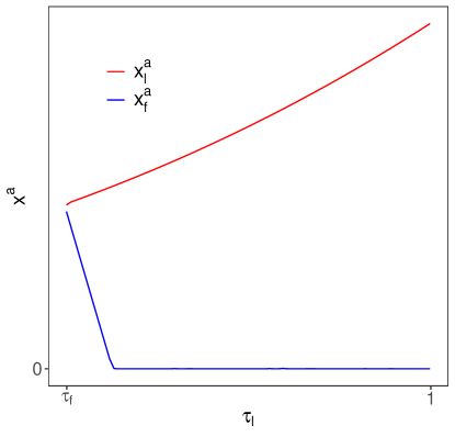
Figure 1: $\tau_{l}$ and $\tau_{f}$ denote the bandwidths of opinion leaders and followers; $x_{l}^{a}$ and $x_{f}^{a}$ denote their levels of informedness in equilibrium: $\tau_{f}=0.16$, $\lambda_{l}=\lambda_{f}=10$, the numbers of opinion leaders and followers are 10 and 90, respectively.

Part (i) of Theorem 3 shows that increasing a player’s bandwidth raises his informedness and influence as a secondary source, and so promotes him to become an opinion leader. More surprisingly, the change diminishes the informedness and influence of any other player, who thus becomes an opinion follower. As depicted in Figure 1 of Appendix B, this equilibrium mechanism may magnify even a small difference between people’s bandwidths into a very uneven distribution of opinions, whereby some people occupy the center of attention, whereas others are barely visible. An important feature of today’s news landscape is that while most Americans express curiosity in many topics such as science, economy, and politics, only a minority of them are willing to spend serious time on hard news consumption (Prior, 2007; Funk et al., 2017). According to Theorem 3(i), this attention gap between the majority and minority may lead the former to consume most firsthand news, and the latter to rely mainly on the secondhand opinions that the former pass along to them. Patterns consistent with this prediction, such as the law of the few and fat-tailed distributions of opinions, have recently been detected in the social media sphere (Lu et al., 2014; Del Vicario et al., 2016; Néda et al., 2017).

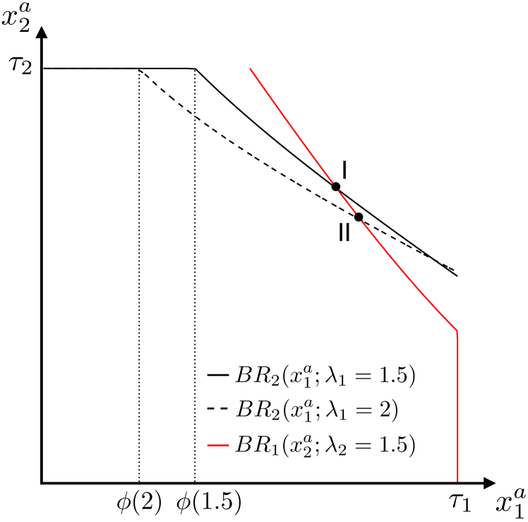
(a) Increase $\lambda_{1}$ from $1.5$ to $2$.

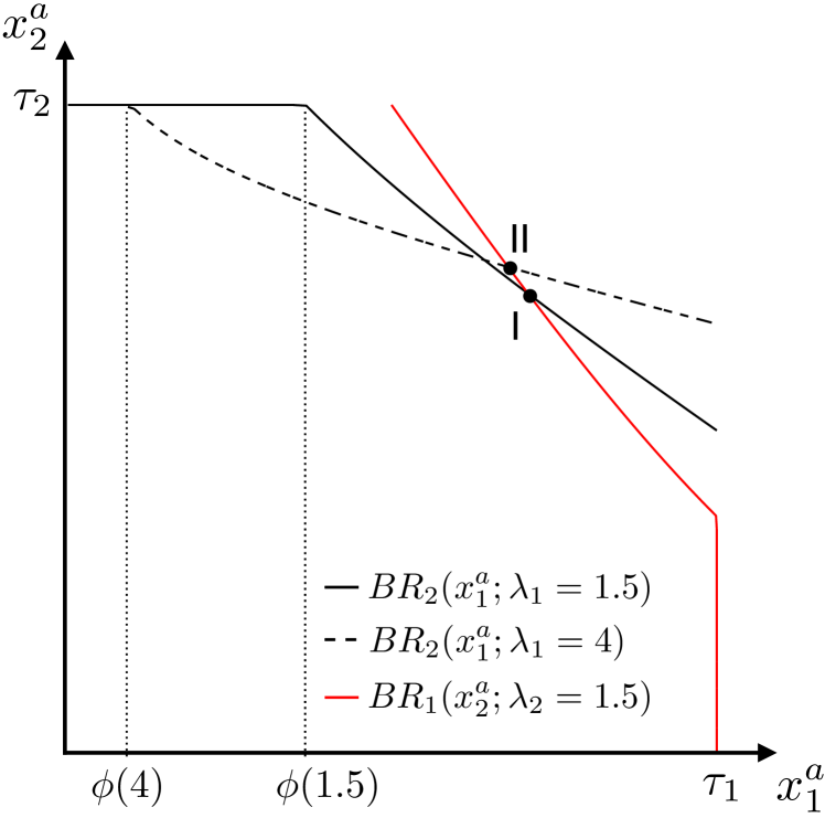
(b) Increase $\lambda_{1}$ from $1.5$ to $4$.

Figure 2: The red and black curves represent player $1$ and player $2$’s best response functions, respectively: $\lambda_{2}=1.5$, $\tau_{1}=\tau_{2}=3$.

Part (ii) of Theorem 3 shows that increasing a player’s visibility parameter by a small amount may promote his informedness and influence while diminishing that of other players. But the opposite can also happen; alternatively, the effect may be neutral. Two countervailing effects are at work here. On the one hand, raising player $i$’s visibility parameter $\lambda_{i}$ reduces the threshold $\phi(\lambda_{i})$ he must cross before starting to exert influences on the other players (recall from Observation 1 that $\phi^{\prime}<0$). We refer to this effect as the intercept effect. On the other hand, as player $i$ becomes a better information disseminator, the amount of attention his friends pay to him no longer varies as sensitively with his informedness as it used to. We refer to this effect as the slope effect, and note that it goes in the opposite direction of the intercept effect. In general, either effect can dominate the other (as depicted in Figure 2 of Appendix B), which renders the comparative statics ambiguous. To counter the rising threat from misinformation and fake news, many social media companies have taken measures that operate through modulating users’ visibility. Among others, Facebook imposes a daily posting limit of 25 articles, beyond which the reach of the posts will be negatively affected. Theorem 3(ii) warns that such measures may backfire and, as demonstrated in the next paragraph, undermine consumer welfare, if they are not calibrated exactly according to the underlying environment.

Part (iii) of Theorem 3 examines the amount of attention that the entire echo chamber pays to the primary source, which is a crucial determinant of players’ equilibrium expected utilities. In general, nothing clear-cut can be said, which is unsurprising given how few assumptions we have made about the magnitudes of the strategic substitution effects. Policy-wise, this finding suggests that the aforementioned interventions could entail ambiguous welfare consequences, and so should be implemented with caution and care. When players are homogeneous, our predictions are clear: increasing a player’s bandwidth makes everyone in the echo chamber better off. As for the consequences of raising a player’s visibility parameter, our result depends on whether that player ends up being an opinion leader or an opinion follower: the entire echo chamber pays less attention to the primary source in the first case, and more attention to the primary source in the second case.

Proof sketch.

Proving Theorem 3 requires a new method we now develop. Due to space limitations, we only sketch the proof for $\partial x_{1}^{a}/\partial\tau_{1}>0$ and $\partial x_{j}^{a}/\partial\tau_{1}<0$ $\forall j\neq 1$, starting from the case of two players. In that case, differentiating the system of equations governing players’ equilibrium informedness against $\tau_{1}$ yields

$$\begin{bmatrix}1&\frac{\partial x_{1}^{2}}{\partial x_{2}^{a}}\\ \frac{\partial x_{2}^{1}}{\partial x_{1}^{a}}&1\end{bmatrix}\begin{bmatrix}\frac{\partial x_{1}^{a}}{\partial\tau_{1}}\\ \frac{\partial x_{2}^{a}}{\partial\tau_{1}}\\ \end{bmatrix}=\begin{bmatrix}1\\ 0\end{bmatrix},$$

where the term $\partial x_{i}^{j}/\partial x_{j}^{a}$ captures how perturbing player $j$’s informedness affects his influence on player $i$. Write $g_{j}$ for $h_{x}(x_{j}^{a};\lambda_{j})$, and recall that

$$\frac{\partial x_{i}^{j}}{\partial x_{j}^{a}}\underbrace{=}_{\text{Theorem \ref{thm_main2}}}g_{j}\underbrace{\in}_{\text{Observation \ref{obs_function}}}\left(0,1\right),$$

i.e., increasing player $j$’s informedness by one unit raises his influence on player $i$ by less than one unit. From $g_{j}>0$, i.e., investments in informedness are strategic substitutes, it follows that in order for the perturbation to have zero net effect on player 2’s bandwidth, it must cause one and only one player to pay more attention to the primary source. Then from $g_{j}<1$, i.e., the strategic substitution effects are sufficiently mild, it follows that player $1$ must pay more attention to the primary source, as the direct effect stemming from increasing his bandwidth dominates the indirect effects that he and player 2 could exert on each other.

Extending the above argument to more than two players is a nontrivial task, as it requires that we trace out how the strategic substitution effects reverberate across a large and endogenous attention network. Mathematically, we must solve

$$\left[\mathbf{I}_{N}+\mathbf{G}_{N}\right]\nabla_{\tau_{1}}\left[x_{1}^{a}\text{ }\cdots\text{ }x_{N}^{a}\right]^{\top}=\left[1\text{ }0\cdots 0\right]^{\top},$$

where $\mathbf{I}_{N}$ is the $N\times N$ diagonal matrix, and $\mathbf{G}_{N}$ is the marginal influence matrix defined as

$$\left[\mathbf{G}_{N}\right]_{i,j}\coloneqq\begin{cases}0&\text{ if }i=j,\\ \frac{\partial x_{i}^{j}}{\partial x_{j}^{a}}&\text{ else. }\end{cases}$$

A seemingly innocuous fact proves its usefulness here, namely an individual attracts the same amount of attention from all his friends, i.e., $x_{i}^{j}\equiv h(x_{j}^{a};\lambda_{j})$ $\forall i\neq j$. Taking derivatives yields $\partial x_{i}^{j}/\partial x_{j}^{a}\equiv g_{j}$ $\forall i\neq j$, i.e., the off-diagonal entries of $\mathbf{G}_{N}$ are constant column by column:

$$\mathbf{G}_{N}=\begin{bmatrix}0&g_{2}&\cdots&g_{N}\\ g_{1}&0&\cdots&g_{N}\\ \vdots&\vdots&\ddots&\vdots\\ g_{1}&g_{2}&\cdots&0\end{bmatrix}.$$

Based on this fact, as well as $g_{j}\in\left(0,1\right)$ $\forall j\in\{1,\cdots,N\}$, we develop a method for solving $[\mathbf{I}_{N}+\mathbf{G}_{N}]^{-1}$ and determining the signs of its entries. Our findings are reported in the next lemma, from which Theorem 3 follows.

Lemma 2.

Fix any $N\geq 2$ and $g_{1},\cdots,g_{N}\in(0,1)$, and let $[\mathbf{G}_{N}]_{i,j}=g_{j}$ $\forall i\neq j$ in the marginal influence matrix. Then $\mathbf{A}_{N}\coloneqq\mathbf{I}_{N}+\mathbf{G}_{N}$ is invertible and satisfies $\forall i\in\left\{1,\cdots,N\right\}$: (i) $\left[\mathbf{A}_{N}^{-1}\right]_{i,i}>0$; (ii) $\left[\mathbf{A}_{N}^{-1}\right]_{i,j}<0$ $\forall j\neq i$;(iii) $\sum_{j=1}^{N}\left[\mathbf{A}_{N}^{-1}\right]_{i,j}>0$.

To the best of our knowledge, Lemma 2 is to new to the literature on network games with strategic substitutes. It generates sharp comparative statics predictions without invoking the usual assumptions made in the literature, such as linear best response functions or a symmetric influence matrix. The lemma is useful for other purposes, such as evaluating the consequences of a common shock to players’ characteristics; see online Appendix O.2 for such an exercise. While the assumption that an individual must be equally visible to all his friends is certainly crucial, it can be relaxed as long as the environment is sufficiently close to the one considered above (as shown in Online Appendix O.6).

4.2 Population size

This section examines the comparative statics regarding players’ population size $N$. To obtain the sharpest insights, we assume, unlike in the previous section, that type $A$ players are homogeneous. Under this assumption, it is easy to see that if the game among type $A$ players has a unique equilibrium (as required by Assumption 1), it must be symmetric. Let $x\left(N\right)$ denote the amount of attention that a typical player pays to the primary source in that equilibrium. The next proposition investigates the comparative statics of $x(N)$.

Proposition 1.

Take any $\lambda,\tau>0$, and $N^{\prime\prime}>N^{\prime}\geq 2$ such that the game among $N\in\left\{N^{\prime},N^{\prime\prime}\right\}$ type $A$ players with visibility parameter $\lambda$ and bandwidth $\tau$ satisfies Assumption 1. As $N$ increases from $N^{\prime}$ to $N^{\prime\prime}$, $x\left(N\right)$ decreases, whereas $Nx\left(N\right)$ may either increase or decrease.

As an echo chamber grows in size, each member of it has access to more secondary sources and so pays less attention to the primary source. Depending on the severity of the free-riding problem compared to the population size effect, the overall effect on the total amount of attention paid by the echo chamber to the primary source and, hence, players’ equilibrium expected utilities, is in general ambiguous (as confirmed by numerical analysis).

Recently, several information platforms, including Allsides.com, have been built to combat the rising polarization through exposing users to diverse viewpoints from both sides. In Online Appendix O.2, we model such a platform as a mega source that results from merging the $A$-revealing source and $B$-revealing source together. We find that the use of a mega source does achieve its purpose: it dissolves echo chambers by forcing different types of players to attend to each other as secondary sources. Yet increasing access to secondary sources discourages information acquisition from primary sources and so exacerbates the free-riding problem. In a symmetric society, merging biased primary sources into a mega source is mathematically equivalent to doubling the population of type $A$ players in Proposition 1. Its effect on equilibrium expected utilities is in general ambiguous.

5 Extensions

This section reports main extensions of the baseline model beyond the ones we have already discussed. Due to space constraints, we postpone the analysis to the online appendix, and focus here on results and implications.

(In)efficiency of echo chambers.

In Online Appendix O.1, we characterize the efficient attention network that maximizes the utilitarian welfare of a symmetric society. We focus on the situation where players are sufficiently biased, and so making one’s default decision in event $\mathcal{U}_{i}$ is efficient. The main qualitative difference between the efficient attention network and an echo chamber equilibrium is, then, that the former can mandate that all players attend to both primary sources. In this way, a lot more players are qualified as secondary sources, despite that each individual cares only about the information generated by one primary source. Such an allocation is efficient when players have large bandwidths and high visibility parameters, and so are good at absorbing information and disseminating it to the others as secondary sources. Yet it cannot be sustained in any equilibrium, because a self-interested individual would gather information about either state $A$ or $B$, but not both.

General primary sources.

In Online Appendix O.2, we extend the baseline model to multiple primary sources with general visibility parameters. The framework therein nests many interesting situations as special cases. For example, if a source is visible to all players in both states, then it is the mega source discussed toward the end of Section 4.2. If it is only visible to a single player in a single state, then it is a private experiment conducted by that player.

Two findings are noteworthy. First, introducing multiple identical and independent primary sources into the model does not affect the total amount of attention one pays to each kind of source. All it does is to dilute players’ attention across the same kind of sources. In our leading example, this finding suggests that increasing the number of independent experiments without improving their qualities may have limited impacts on public opinion and consumer welfare.

Second, when the visibility parameter of primary sources differs from one, we must rescale things properly to make the previous equilibrium characterizations work. As for comparative statics, we find that increasing the visibility of primary sources effectively diminishes the visibility of all secondary sources. Then using the toolkit developed in Lemma 2, we find the same ambiguous effect as in Theorem 3(ii). Thus in practice, factors that affect primary sources’ visibility — such as the increasing reliance of scientific journals on digital technologies and AI to boost distribution and reach — could have ambiguous effects on public opinion and consumer welfare.

6 Further Application

This section studies a political economy application of our model.

Example 3.

Each player $i\in\mathcal{I}$ is either a Democratic voter or a Republican voter. He must vote between a Democratic candidate or a Republican candidate, $d_{i}\in\{L,R\}$, whose qualities are uncertain $\omega\in\{L,R\}$. Voting for the best quality candidate generates the highest instrumental value, whereas voting for the lowest quality candidate takes a mental toll. The latter’s magnitude differs, depending whether the vote goes to one’s own-party candidate or the opposing party candidate. Instrumental voting is an important motive for consuming political news (Prat and Strömberg, 2013).

Original reporting of the state is generated by two primary sources called $L$-revealing and $R$-revealing. The $\omega$-revealing source announces a “newsworthy message” in state $\omega$, and an “ideological message” in state $\omega^{\prime}\neq\omega$. As in Che and Mierendorff (2019), we interpret the $R$-revealing source as a liberal newspaper, say the NYTimes. Its endorsement for the Republican candidate in state $R$ sends a surprising signal to the electorate and, according to Chiang and Knight (2011), is the most effective in shaping voter’s beliefs and decisions. The reporting of state $L$, on the other hand, conforms with the newspaper’s ideology, hence the name “ideological message.”

The game begins with voters specifying how much attention to pay to each primary source and to each other. After that, messages about the state first transmit from the primary sources to voters, and then between voters themselves. Whenever an attention channel gets interrupted, the receiver gets an ideological message. To interpret, consider a reader with a gut feeling that the NYTimes’ reporting is pro-liberal. As he parses the content, he may realize its pro-conservative nature and react accordingly. Such a success cannot be guaranteed, however, as the reader has limited attention and is prone to information transmission failure.

Voters may differ in their bandwidth $\tau_{i}$s, depending on their opportunity costs of consuming hard news (Prior, 2007). They may also differ in their visibility parameter $\lambda_{i}$s; indeed, the famous “Oprah effect” indicates that public figures like Oprah Winfrey are more capable of deciphering and disseminating the complex messages of elite newspapers to the less educated audience than ordinary people, in addition to being enchanting to watch (Baum and Jamison, 2006). $\hfill\diamondsuit$

Our analysis raises the possibility of sustaining echo chambers among rationally inattentive voters who consume political news for instrumental reasons. In practice, voters may derive intrinsic values from consuming ideological content, or they may seek confirming information due to biased belief updating. To the extent that these forces tend to aggravate, rather than mitigate, opinion segregation, Theorem 1 prescribes a lower bound for the degree of opinion segregation that may arise in practice.

After playing an echo chamber equilibrium, the majority of our voters will have more faith in their own-party candidate than before, whereas a minority of them feels strongly about supporting the opposing party candidate. The coexistence of a belief polarization and an occasional, drastic, belief reversal is a hallmark of Bayesian rationality. Suggestive evidence for each individual phenomenon has been documented separately by several authors (as discussed in Footnote 7), although we are unaware of any study that accounts for both phenomena simultaneously.

Our analysis adds to the policy debate surrounding several current events. In the aftermath of the 2021 U.S. Capitol attack, there have been calls to modify Section 230 of the Communications Decency Act of 1996, so as to allow Internet companies to exercise more account control (Romm, 2021). We caution that controls via modulating account visibility may backfire if they are not calibrated exactly according to underlying environment. The FCC’s viewpoint diversity objectives and, more specifically, the eight voice rule, mandate that at least eight independent media outlets must be operating in the same digital media area (Ho and Quinn, 2008). As discussed in Section 5 (and formally shown in Online Appendix O.2), increasing the number of independent primary sources without improving their qualities has no real impact on players’ equilibrium strategies and utilities in our model.

7 Concluding remarks

This paper develops a rational inattention theory of echo chamber. To single out the economic forces of our interest, we abstract away from alternative considerations such as strategic players whose goal is to persuade, manipulate, or confuse other people. Our model can be interpreted as a microfoundation for homophily as the equilibrium mode of information transmission between rationally inattentive decision makers. The friction of our interest — namely the disruption of communication due to RI — differs from those that have been studied by the existing literature on learning over homophilous social networks (see, e.g., Golub and Jackson 2012 for DeGroot learning, and Lobel and Sadler 2016 for social learning). These alternative considerations and forces are certainly important in shaping the way our society functions. Integration them into our work and, more broadly, the study of echo chambers, is an intriguing topic for future research.

Appendix A Proofs

A.1 Useful lemmas and their proofs

Proof of Lemma 1.

When players can attend to the primary sources but not to each other, the ex ante problem faced by a type $A$ player (call him $i$) who plans to make decision $A$ in event $\mathcal{U}_{i}$ is

$$\max_{x^{a},x^{b}}-\frac{\beta_{i}}{2}\exp(-x^{a})\text{ s.t. }x^{a},x^{b}\geq 0\text{ and }\tau_{i}\geq x^{a}+x^{b}.$$

If, instead, the player plans to make decision $B$ in event $\mathcal{U}_{i}$, then his ex ante problem becomes

$$\max_{x^{a},x^{b}}-\frac{1}{2}\exp(-x^{b})\text{ s.t. }x^{a},x^{b}\geq 0\text{ and }\tau_{i}\geq x^{a}+x^{b}.$$

The solutions to these problems are $(x^{a},x^{b})=(\tau_{i},0)$ and $(x^{a},x^{b})=(0,\tau_{i})$, respectively. The first solution generates a higher expected utility than the second and so is optimal. ∎

Proof of Lemma 2.

We proceed in three steps.

Step 1.

Solve for $\mathbf{A}_{N}^{-1}$. We conjecture that

$$\text{det}\left(\mathbf{A}_{N}\right)=1+\sum_{s=1}^{N}\left(-1\right)^{s-1}\left(s-1\right)\sum_{\begin{subarray}{c}\left(k_{l}\right)_{l=1}^{s}:k_{l}\in\{1,\cdots,N\},\\ k_{1}<\cdots<k_{s}\end{subarray}}\prod_{l=1}^{s}g_{k_{l}},$$ (1)

and that the following hold for all $i\in\{1,\cdots,N\}$ and $j\in\{1,\cdots,N\}-\{i\}$:

$$\left[\mathbf{A}_{N}^{-1}\right]_{i,i}=\frac{1}{\text{det}\left(\mathbf{A}_{N}\right)}[1+\sum_{s=1}^{N-1}\left(-1\right)^{s-1}\left(s-1\right)\sum_{\begin{subarray}{c}\left(k_{l}\right)_{l=1}^{s}:k_{l}\in\left\{1,\cdots,N\right\}-\left\{i\right\},\\ k_{1}<\cdots<k_{s}\end{subarray}}\prod_{l=1}^{s}g_{k_{l}}]$$ (2)

and

$$\left[\mathbf{A}_{N}^{-1}\right]_{i,j}=\frac{-g_{j}}{\text{det}\left(\mathbf{A}_{N}\right)}\prod_{k\in\left\{1,\cdots,N\right\}-\left\{i,j\right\}}\left(1-g_{k}\right).$$ (3)

We omit most algebra, but note that $\mathbf{A}_{N}$ can be rewritten as $\mathbf{B}_{N}+\mathbf{u}_{N}\mathbf{v}_{N}^{\top},$ where $\mathbf{B}_{N}\coloneqq\text{diag}(1-g_{1}\text{ }\cdots\text{ }1-g_{N})$, $\mathbf{u}_{N}$ is the $N$-vector of ones, and $\mathbf{v}_{N}\coloneqq[g_{1}\text{ }\cdots\text{ }g_{N}]^{\top}$. Since $\mathbf{A}_{N}$ is a rank-one update of an invertible matrix $\mathbf{B}_{N}$, its inverse can be obtained from applying the Sherman-Morrison formula (Sherman and Morrison, 1950):

$$\mathbf{A}_{N}^{-1}=\mathbf{B}_{N}^{-1}-\frac{\mathbf{B}_{N}^{-1}\mathbf{u}_{N}\mathbf{v}_{N}^{\top}\mathbf{B}_{N}^{-1}}{1+\mathbf{v}_{N}^{\top}\mathbf{B}_{N}^{-1}\mathbf{u}_{N}}.$$

Simplifying the last expression by doing lengthy algebra gives the desired result.

Step 2.

Show that $\text{det}\left(\mathbf{A}_{N}\right)>0$, i.e,

$$\sum_{s=1}^{N}\left(-1\right)^{s-1}\left(s-1\right)\sum_{\begin{subarray}{c}\left(k_{l}\right)_{l=1}^{s}:k_{l}\in\left\{1,\cdots,N\right\},\\ k_{1}<\cdots<k_{s}\end{subarray}}\prod_{l=1}^{s}g_{k_{l}}>-1.$$

Denote the left-hand side of the above inequality by $\text{LHS}\left(g_{1},\cdots,g_{N}\right)$. Since the function $\text{LHS}:[0,1]^{N}\rightarrow\mathbb{R}$ is linear in each $g_{i}$, holding $(g_{j})_{j\neq i}$ constant, its minimum is attained at an extremal point of $[0,1]^{N}$. Indeed, since the function is symmetric across $g_{i}$s, the following hold for any $\left(g_{1},\cdots,g_{N}\right)\in\left\{0,1\right\}^{N-1}$ such that $\sum_{i=1}^{N}g_{i}=n$:

$$\text{LHS}\left(g_{1},\cdots,g_{N}\right)=f\left(n\right)\coloneqq\sum_{k=1}^{n}\left(-1\right)^{k-1}\left(k-1\right){n\choose k}.$$

It remains to show that $f\left(n\right)\geq-1$ $\forall n=0,1,\cdots,N$. When $n=0$ and $1$, $f(n)=0>-1$, as conjectured. For each $n\geq 2$, define

$$p\left(n\right)\coloneqq\sum_{k=1}^{n}\left(-1\right)^{k}k{n\choose k}.$$

Below we prove by induction that $f\left(n\right)=-1$ and $p\left(n\right)=0$ for all $n=2,\cdots,N$.

Our conjecture is clearly true when $n=2$:

$$f\left(2\right)=-{2\choose 2}=-1\text{ and }p\left(2\right)=-{2\choose 1}+2{2\choose 2}=0.$$

In the case it is true for any $n\geq 2$, the following must hold for $n+1$:

$$f\left(n+1\right)$$

$$=\sum_{k=1}^{n+1}\left(-1\right)^{k-1}\left(k-1\right){n+1\choose k}$$

$$=\sum_{k=1}^{n}\left(-1\right)^{k-1}\left(k-1\right){n+1\choose k}+\left(-1\right)^{n}n{n+1\choose n+1}$$

$$=\sum_{k=1}^{n}\left(-1\right)^{k-1}\left(k-1\right)\left({n\choose k}+{n\choose k-1}\right)+\left(-1\right)^{n}n \because{n+1\choose k}={n\choose k}+{n\choose k-1}$$ ()

$$=f\left(n\right)+0{n\choose 0}+\sum_{k=1}^{n-1}\left(-1\right)^{k}k{n\choose k}+\left(-1\right)^{n}n{n\choose n}$$

$$=f\left(n\right)+p\left(n\right)$$

$$=-1,$$

and

$$p\left(n+1\right)$$

$$=\sum_{k=1}^{n+1}\left(-1\right)^{k}k{n+1\choose k}$$

$$=\sum_{k=1}^{n}\left(-1\right)^{k}k\left({n\choose k}+{n\choose k-1}\right)+\left(-1\right)^{n+1}\left(n+1\right) \because{n+1\choose k}={n\choose k}+{n\choose k-1}$$ ()

$$=p\left(n\right)+\sum_{k=0}^{n-1}\left(-1\right)^{k+1}\left(k+1\right){n\choose k}+\left(-1\right)^{n+1}\left(n+1\right)$$

$$=0+\sum_{k=1}^{n-1}\left(-1\right)^{k+1}k{n\choose k}+\sum_{k=0}^{n-1}\left(-1\right)^{k+1}{n\choose k}+\left(-1\right)^{n+1}\left(n+1\right).$$

Then from

$$\sum_{k=1}^{n-1}\left(-1\right)^{k+1}k{n\choose k} =\sum_{k=1}^{n}\left(-1\right)^{k+1}k{n\choose k}-(-1)^{n+1}n$$

$$=-p\left(n\right)-(-1)^{n+1}n$$

$$=-(-1)^{n+1}n,$$

it follows that

$$p\left(n+1\right)=\sum_{k=0}^{n-1}\left(-1\right)^{k+1}{n\choose k}+\left(-1\right)^{n+1},$$

and so $p(n+1)=0$ if and only if

$$q\left(n\right)\coloneqq\sum_{k=0}^{n-1}\left(-1\right)^{k+1}{n\choose k}=\left(-1\right)^{n}.$$

To verify the last condition, we distinguish between whether $n$ is odd or even. In the first case, simplifying $q(n)$ using the fact that

$$(-1)^{k+1}{n\choose k}+(-1)^{n-k+1}{n\choose n-k}=0\text{ }\forall k\in\{1,\cdots,n-1\},$$

yields

$$q(n)=(-1){n\choose 0}+0=(-1)^{n},\text{ as desired}.$$

In the second case, expanding $q\left(n\right)$ yields

$$q\left(n\right) =\sum_{k=1}^{n-1}\left(-1\right)^{k-1}\left({n-1\choose k-1}+{n-1\choose k}\right)-{n\choose 0} \because{n\choose k}={n-1\choose k-1}+{n-1\choose k}$$ ()

$$=\sum_{k=1}^{n-1}\left(-1\right)^{k-1}{n-1\choose k-1}+\sum_{k=0}^{n-1}\left(-1\right)^{k-1}{n-1\choose k}. \because-{n\choose 0}=(-1)^{-1}{n-1\choose 0}$$ ()

Then from

$$\sum_{k=1}^{n-1}\left(-1\right)^{k-1}{n-1\choose k-1}=\sum_{k=0}^{n-2}\left(-1\right)^{k}{n-1\choose k}=-q\left(n-1\right)=1$$

and

$$\sum_{k=0}^{n-1}\left(-1\right)^{k-1}{n-1\choose k} =\sum_{k=0}^{n-2}\left(-1\right)^{k-1}{n-1\choose k}+(-1)^{n-2}{n-1\choose n-1}$$

$$=q\left(n-1\right)+1$$

$$=0,$$

it follows that $q\left(n\right)=1=\left(-1\right)^{n}$, as desired.

Step 3.

Verify that $\left[\mathbf{A}_{N}^{-1}\right]_{i,i}>0$, $\left[\mathbf{A}_{N}^{-1}\right]_{i,j}<0$, and $\sum_{j=1}^{N}\left[\mathbf{A}_{N}^{-1}\right]_{i,j}>0$ for all $i\in\{1,\cdots,N\}$ and $j\in\{1,\cdots,N\}-\{i\}$.

$\left[\mathbf{A}_{N}^{-1}\right]_{i,j}$ is clearly negative. To show that $[\mathbf{A}^{-1}_{N}]_{i,i}$ is positive, define $\mathbf{D}_{N,i}$ as the principal minor of $\mathbf{A}_{N}$ that obtains from deleting the $i^{th}$ row and column of $\mathbf{A}_{N}$. Since $\mathbf{D}_{N,i}$ satisfies all the properties listed in Lemma 2, $\text{det}\left(\mathbf{D}_{N,i}\right)$ must be positive by Step 2. Then from the fact that $\left[\mathbf{A}_{N}^{-1}\right]_{i,i}=\text{det}\left(\mathbf{D}_{N,i}\right)/\text{det}\left(\mathbf{A}_{N}\right)$, it follows that $[\mathbf{A}_{N}^{-1}]_{i,i}>0$, as desired. Finally, summing $\left[\mathbf{A}_{N}^{-1}\right]_{i,j}$ over $j\in\left\{1,\cdots,N\right\}$ and doing lengthy algebra yields

$$\sum_{j=1}^{N}\left[\mathbf{A}_{N}^{-1}\right]_{i,j}=\frac{1}{\text{det}\left(\mathbf{A}_{N}\right)}\prod_{k\in\left\{1,\cdots,N\right\}-\{i\}}\left(1-g_{k}\right)>0,\text{ as desired}.\qed$$

The next lemma expands on Observation 1. It provides a full list of the properties of functions $\phi$ and $h$, as defined in Definition 5.

Lemma 3.

$\phi^{\prime}(\lambda)<0$ on $\left(1,+\infty\right)$ and $\lim_{\lambda\downarrow 1}\phi(\lambda)=+\infty$. For each $\lambda>1$, $h(\cdot;\lambda)$ satisfies (i) $h\left(\phi\left(\lambda\right);\lambda\right)=0$; (ii) $h_{x}\left(x;\lambda\right)\in\left(0,1\right)$ on $(\phi\left(\lambda\right),+\infty)$ and $\lim_{x\downarrow\phi(\lambda)}h_{x}(x;\lambda)=1$; and (iii) $h_{xx}\left(x,\lambda\right)<0$ on $(\phi\left(\lambda\right);+\infty)$.

Proof.

The result follows from straightforward algebra. ∎

Lemma 4.

Fix any $\lambda>1$ and $\tau>\phi(\lambda)$. For each $N\geq 2$ and $x\in[\phi(\lambda),+\infty)$, define

$$\varphi^{N}\left(x\right)\coloneqq\tau-(N-1)h(x;\lambda).$$

Then $\varphi^{N}$ has a unique fixed point $x(N)$ that satisfies $x(N)\in(\phi(\lambda),\tau)$, $\lim_{N\rightarrow+\infty}x(N)\\ =\phi(\lambda)$, $\lim_{\tau\rightarrow+\infty}x(N)=+\infty$, and $dx(N)/d\tau\in(1/N,1)$.

Proof.

Since $h(\phi(\lambda);\lambda)=0$ and $h_{x}(x;\lambda)>0$ on $(\phi(\lambda),+\infty)$ by Lemma 3, $\varphi^{N}(x)=\tau-(N-1)h(x;\lambda)$ has a unique fixed point $x(N)$ that belongs to $(\phi(\lambda),\tau)$ (drawing a picture makes this point clear). In order to satisfy $x(N)=\varphi^{N}(x(N))>\phi(\lambda)$, $h(x(N);\lambda)$ must converge to zero as $N\rightarrow+\infty$, which, together with Lemma 3, implies that $\lim_{N\rightarrow+\infty}x(N)=\phi(\lambda)$.

Turning to the relationship between $x(N)$ and $\tau$, notice that $x(N)$ must grow to infinity as $\tau\rightarrow+\infty$ in order to satisfy $x(N)+(N-1)h(x(N);\lambda)=\tau$. Meanwhile, taking the total derivative of $\varphi^{N}(x(N))=x(N)$ with respect to $\tau$ yields $dx(N)/d\tau=[1+(N-1)h_{x}(x(N);\lambda)]^{-1}$. The last term lies in $(1/N,1)$ because $h_{x}\in(0,1)$. ∎

A.2 Proofs of theorems and propositions

Proof of Theorems 1(i) and 2.

We proceed in four steps.

Step 1.

Show that for any type $A$ player (call him $i$), making the default decision in event $\mathcal{U}_{i}$ is a dominant strategy when $\beta_{i}$ is sufficiently small.

If player $i$ attends only to source $a$ and makes decision $A$ in event $\mathcal{U}_{i}$, then his ex ante expected utility equals $-\beta_{i}\exp\left(-\tau_{i}\right)/2.$ If, instead, he makes decision $B$ in event $\mathcal{U}_{i}$, then his ex ante expected utility is at most $-\exp(-\overline{\lambda}\tau_{i})/2$, where $\overline{\lambda}\coloneqq\max\{1,\lambda_{j},j\in\mathcal{I}-\{i\}\}$. The reason is that in a hypothetical situation where all the other players knows for sure when state $A$ has occurred, player $i$ essentially faces the original primary source $b$, together with $|\mathcal{I}|-1$ primary sources with visibility parameter $\lambda_{j}$s, $j\neq i$. His optimal strategy is to focus on the source with the highest visibility parameter $\overline{\lambda}$; the resulting ex ante expected utility equals $-\exp(-\overline{\lambda}\tau_{i})/2$. The last term is smaller than $-\beta_{i}\exp\left(-\tau_{i}\right)/2$ when $\beta_{i}<\exp((1-\overline{\lambda})\tau_{i})$. The remainder of the proof assumes that this is the case.

Step 2.

Show that any equilibrium must be an echo chamber equilibrium. It suffices to show that $x_{i}^{b}=0$ and $x_{i}^{j}=0$ $\forall i\in\mathcal{A}$ and $j\in\mathcal{B}$. Fix any $x_{-i}\in\mathcal{X}_{-i}$. Rewrite player $i$’s problem: $\max_{x_{i}\in\mathcal{X}_{i}}-\beta_{i}\mathbb{P}_{x}(\mathcal{U}_{i}\mid\omega=B)/2$, as follows:

$$\max_{(x_{i}^{c})_{c\in\mathcal{C}_{i}}} -x_{i}^{a}-\sum_{j\in\mathcal{I}-\{i\}}\log(\delta_{j}^{a}+(1-\delta_{j}^{a})\delta_{i}^{j})$$ (4)

s.t. $$x_{i}^{c}\geq 0\text{ }\forall c\in\mathcal{C}_{i}\text{ and }\tau_{i}\geq\sum_{i\in\mathcal{C}_{i}}x_{i}^{c},$$

where $\delta_{i}^{a}\coloneqq\exp(-x_{i}^{a})$ and $\delta_{i}^{j}\coloneqq\exp(-\lambda_{j}x_{i}^{j})$. Since (4) is a concave problem, it can be solved using the Lagrangian method. Let $\eta_{x_{i}^{c}}\geq 0$ and $\gamma_{i}\geq 0$ denote the Lagrange multipliers associated with $x_{i}^{c}\geq 0$ and $\tau_{i}\geq\sum_{c\in\mathcal{C}_{i}}x_{i}^{c}$, respectively. The first-order conditions regarding $x_{i}^{a}$, $x_{i}^{b}$, and $x_{i}^{j}$, $j\in\mathcal{I}-\{i\}$, are

$$1-\gamma_{i}+\eta_{x_{i}^{a}} =0, {}_{x_{i}^{a}}$$ (FOC)

$$-\gamma_{i}+\eta_{x_{i}^{b}} =0, {}_{x_{i}^{b}}$$ (FOC)

$$\text{and }\frac{\lambda_{j}(1-\delta_{j}^{a})\delta_{i}^{j}}{\delta_{j}^{a}+(1-\delta_{j}^{a})\delta_{i}^{j}}-\gamma_{i}+\eta_{x_{i}^{j}} =0, {}_{x_{i}^{j}}$$ (FOC)

respectively. FOC${}_{x_{i}^{a}}$ and FOC${}_{x_{i}^{b}}$ together imply that $\gamma_{i}=\eta_{x_{i}^{b}}\geq 1>0$, and, in turn, that $\sum_{c\in\mathcal{C}_{i}}x_{i}^{c}=\tau_{i}$ and $x_{i}^{b}=0$. In words, player $i$ must exhaust his bandwidth but ignore source $b$. The opposite is true for any type $B$ player $j$, who must ignore source $a$, i.e., $x_{j}^{a}=0$. Letting $\delta_{j}^{a}\coloneqq\exp(-x_{j}^{a})=1$ in FOC${}_{x_{i}^{j}}$ yields $\eta_{x_{i}^{j}}=\gamma_{i}>0$ and, hence, $x_{i}^{j}=0$.

Step 3.

Characterize the equilibrium attention network(s) among type $A$ players. Simplifying FOC${}_{x_{i}^{j}}$ shows that

$$x_{i}^{j}=\frac{1}{\lambda_{j}}\log\max\{\left(\frac{\lambda_{j}}{\gamma_{i}}-1\right)(\exp(x_{j}^{a})-1),1\}\text{ }\forall i\in\mathcal{A}\text{ and }j\in\mathcal{A}-\{i\},$$ (5)

where the term $\gamma_{i}$ in the above expression represents the Lagrange multiplier associated with $x_{i}^{a}\geq 0$. Since $\gamma_{i}\geq 1$, and the inequality is strict if and only if $x_{i}^{a}=0$ (as shown in Step 2), (5) implies that

$$x_{i}^{a}=[\tau_{i}-\sum_{j\in\mathcal{L}-\{i\}}\frac{1}{\lambda_{j}}\log\max\{(\lambda_{j}-1)(\exp(x_{j}^{a})-1),1\}]^{+}\text{ }\forall i\in\mathcal{A}.$$ (6)

Equations (5) and (6) together pin down all equilibria of the game among type $A$ players. They can be further simplified in the following scenarios.

$\bullet$ $x_{i}^{a}>0$ $\forall i\in\mathcal{A}$. In this case, $\gamma_{i}\equiv 1$ $\forall i\in\mathcal{A}$, hence (5) becomes

$$x_{i}^{j}=\frac{1}{\lambda_{j}}\log\max\{(\lambda_{j}-1)(\exp(x_{j}^{a})-1),1\}\text{ }\forall i\in\mathcal{A}\text{ and }j\in\mathcal{A}-\{i\}.$$ (7)

A close inspection of (7) reveals the equivalence between (a) $x_{j}^{a}>\phi(\lambda_{j})$, (b) $x_{i}^{j}>0$, and (c) $x_{k}^{j}\equiv h(x_{j}^{a};\lambda_{j})$ $\forall k\in\mathcal{A}-\{j\}$, thus proving Part (ii) of Theorem 2.

$\bullet$ $x_{i}^{j}>0$ $\forall i\in\mathcal{A}$ and $j\in\mathcal{A}-\{i\}$. In this case (5) and (6) become

$$x_{i}^{j} =h(x_{j}^{a};\lambda_{j})\text{ }\forall i\in\mathcal{A}\text{ and }j\in\mathcal{A}-\{i\}$$ (8)

$$\text{ and }x_{i}^{a} =\tau_{i}-\sum_{j\in\mathcal{A}-\{i\}}h(x_{j}^{a};\lambda_{j})\text{ }\forall i\in\mathcal{A},\text{ respectively}.$$ (9)

Simplifying $\mathbb{P}_{x}\left(\mathcal{U}_{i}\mid\omega=B\right)$ accordingly yields

$$\mathbb{P}_{x}\left(\mathcal{U}_{i}\mid\omega=B\right)$$

$$=\delta_{i}^{a}\prod_{j\in\mathcal{A}-\{i\}}(\delta_{j}^{a}+(1-\delta_{j}^{a})\delta_{i}^{j})$$

$$=\exp(-x_{i}^{a})\prod_{j\in\mathcal{A}-\{i\}}\exp(-x_{j}^{a})+(1-\exp(-x_{j}^{a}))\exp(-\lambda_{j}\cdot\frac{1}{\lambda_{j}}\log(\lambda_{j}-1)(\exp(x_{j}^{a})-1))$$

$$=\exp(-\sum_{j\in\mathcal{A}}x_{j}^{a}+\sum_{j\in\mathcal{A}-\{i\}}\phi\left(\lambda_{j}\right)),$$

thus proving Part (iii) of Theorem 2.

Step 4.

Show that the game among type $A$ players has an equilibrium. As shown in Step 3, all equilibria of this game can be obtained from first solving (6) and then substituting the result(s) into (5). What it remains is to show that (6) admits a solution. For starters, write $\left\{1,\cdots,N\right\}$ for $\mathcal{A}$. Define, for each $\mathbf{x}^{a}\coloneqq[x_{1}^{a}\text{ }\cdots\text{ }x_{N}^{a}]^{\top}\in\times_{i=1}^{N}\left[0,\tau_{i}\right]$, $T(\mathbf{x}^{a})$ as the $N$-vector whose $i^{th}$ entry is given by the right-hand side of (6), and rewrite (6) as $T(\mathbf{x}^{a})=\mathbf{x}^{a}$. Since $T:\times_{i=1}^{N}\left[0,\tau_{i}\right]\rightarrow\times_{i=1}^{N}\left[0,\tau_{i}\right]$ is a continuous mapping from a compact convex set to itself, it has a fixed point according to the Brouwer fixed point theorem. ∎

Proof of Theorem 1(ii).

If $\tau\leq\phi(\lambda)$, then the game has a unique equilibrium whereby all players attend to their own-biased sources but nothing else. The remainder of the proof focuses on the more interesting case where $\tau>\phi(\lambda)$.

Our starting observation is that each player must attend only to a single primary source in any equilibrium. Thus in a symmetric equilibrium, either (i) all type $A$ players attend to source $a$ and their like-minded friends, followed by making decision $A$ in event $\mathcal{U}_{i}$s; or (ii) they all attend to source $b$ and their like-minded friends, followed by making decision $B$ in event $\mathcal{U}_{i}$s.

Part (a): We proceed in two steps.

Step 1.

Show that the game has a unique symmetric equilibrium of the first kind when $N$ is large.

Let $x_{i}^{a}$ and $x_{i}^{j}$ denote the amount of attention that a typical type $A$ player $i$ pays to source $a$ and each like-minded friend of his, respectively. If $x_{i}^{j}=0$, then $x_{i}^{a}=\tau$. But then $x_{j}^{i}=h(\tau,\lambda)\neq x_{i}^{j}$, which violates symmetry. As a result, $x_{i}^{j}>0$ must hold. $x_{i}^{a}$ must solve $x=\tau-(N-1)h(x;\lambda)\coloneqq\varphi^{N}(x)$ and so must equal $x(N)$ by Lemma 4. Substituting the last result into Parts (ii) and (iii) of Theorem 2(ii) yields $x_{i}^{j}=h(x(N);\lambda)>0$, as well as $-\beta\exp\left(-Nx\left(N\right)+\left(N-1\right)\phi\left(\lambda\right)\right)/2$ as the player’s ex ante expected utility.

To sustain the above outcome on the equilibrium path, player $i$ mustn’t benefit from attending to source $b$ and type $B$ players, followed by making decision $B$ in event $\mathcal{U}_{i}$. In case player $i$ commits such a deviation, solving his best response to type $B$ players’ equilibrium strategies yields $y_{i}^{j}=h\left(x\left(N\right);\lambda\right)$ as the amount of attention that he pays to each type $B$ player, and $y_{i}^{b}=\tau-Nh(x(N);\lambda)$ as the amount of attention that he pays to source $b$. The last term is positive when $N$ is large, because $y_{i}^{b}=\varphi^{N}(x(N))-h(x(N);\lambda)=x(N)-h(x(N);\lambda)\rightarrow\phi(\lambda)>0$ as $N\rightarrow\infty$ by Lemma 4. The ex ante expected utility generated by this best response function equals

$$-\frac{1}{2}\exp(-\tau+\frac{N\left(\tau-x\left(N\right)\right)}{N-1}-Nx\left(N\right)+N\phi\left(\lambda\right)).$$ (10)

Comparing (10) with the on-path expected utility, we find that the former is smaller than the latter (and so the deviation is unprofitable) if and only if

$$\frac{\tau}{N-1}+\phi\left(\lambda\right)-\frac{N}{N-1}x\left(N\right)>\log\beta.$$ (11)

Since the left-hand side of (11) converges to zero as $N$ grows to infinity by Lemma 4, it must exceed the right-hand side when $N$ is sufficiently large.

Step 2.

Show that no symmetric equilibrium of the second kind exists. In any equilibrium as such, any type $A$ player can strictly benefit from attending to source $a$ and $N-1$ type $B$ players (who pay $x(N)$ unit of attention to source $a$), followed by making his default decision in event $\mathcal{U}_{i}$.

Part (b): By Lemma 4, the left-hand side of (11), hereinafter denoted by LHS$(\tau)$, satisfies $\lim_{\tau\downarrow\phi(\lambda)}\text{LHS}(\tau)=0$ and $\frac{d\text{LHS}(\tau)}{d\tau}=\frac{1}{N-1}-\frac{N}{N-1}\frac{dx(N)}{d\tau}\in(-1,0)$. Thus there exists $\underline{\tau}\in(\phi(\lambda),+\infty)$ such that (11) holds if and only if $\tau\in(\phi(\lambda),\underline{\tau})$. The remainder of the proof is the same as that of Part (i) and so is omitted for brevity. ∎

Proof of Theorem 3.

Write $\{1,\cdots,N\}$ for $\mathcal{A}$. Since $x_{i}^{a}>\phi(\lambda_{i})$ $\forall i\in\mathcal{A}$ in equilibrium (as required by Assumption 1), $g_{i}\coloneqq h_{x}(x_{i}^{a};\lambda_{i})\in(0,1)$ must hold by Lemma 3. Let $[\mathbf{G}_{N}]_{i,j}=g_{j}$ $\forall j\in\{1,\cdots,N\}$ and $i\in\{1,\cdots,N\}-\{j\}$ in the marginal influence matrix. The corresponding matrix $\mathbf{A}_{N}\coloneqq\mathbf{I}_{N}+\mathbf{G}_{N}$ satisfies the properties stated in Lemma 2.

Part (i): We prove the result for $\tau_{1}$. Under Assumption 1, $(x_{i}^{a})_{i=1}^{N}$ and $(x_{i}^{j})_{i,j}$ must solve (9) and (8) among type $A$ players, respectively. Differentiating (9) with respect to $\tau_{1}$ yields

$$\nabla_{\tau_{1}}\mathbf{x}^{a}=\mathbf{A}_{N}^{-1}\left[1\text{ }0\text{ }\cdots\text{ }0\right]^{\top},$$

where $\mathbf{x}^{a}\coloneqq[x_{1}^{a}\text{ }\cdots\text{ }x_{N}^{a}]^{\top}$. From Lemma 2, it follows that

$$\frac{\partial x_{1}^{a}}{\partial\tau_{1}}=\left[\mathbf{A}_{N}^{-1}\right]_{1,1}>0\text{ and }\frac{\partial x_{j}^{a}}{\partial\tau_{1}}=\left[\mathbf{A}_{N}^{-1}\right]_{j,1}<0\text{ }\forall j\neq 1.$$

Substituting this result into (8) yields

$$\frac{\partial x_{j}^{1}}{\partial\tau_{1}}=g_{1}\frac{\partial x_{1}^{a}}{\partial\tau_{1}}>0\text{ and }\frac{\partial x_{k}^{j}}{\partial\tau_{1}}=g_{j}\frac{\partial x_{j}^{a}}{\partial\tau_{1}}<0\text{ }\forall j\neq 1\text{ and }k\neq j,\text{ as desired}.$$

Part (ii): We prove the result for $\lambda_{1}$. Differentiating (9) with respect to $\lambda_{1}$ yields

$$\nabla_{\lambda_{1}}\mathbf{x}^{a}=\kappa\mathbf{A}_{N}^{-1}\left[0\text{ }1\text{ }\cdots\text{ }1\right]^{\top},$$

where $\kappa\coloneqq-h_{\lambda}(x_{1}^{a};\lambda_{1})$ has an ambiguous sign in general, as confirmed by numerical analysis. From Lemma 2, it follows that

$$\operatorname{sgn}(\frac{\partial x_{1}^{a}}{\partial\lambda_{1}})=\operatorname{sgn}(\kappa\underbrace{\sum_{i\neq 1}\left[\mathbf{A}_{N}^{-1}\right]_{1,i}}_{<0})=\operatorname{sgn}\left(-\kappa\right)$$

and that

$$\operatorname{sgn}(\frac{\partial x_{j}^{a}}{\partial\lambda_{1}})=\operatorname{sgn}(\kappa(\underbrace{\sum_{i=1}^{N}\left[\mathbf{A}_{N}^{-1}\right]_{j,i}}_{>0}-\underbrace{\left[\mathbf{A}_{N}^{-1}\right]_{j,1}}_{<0}))=\operatorname{sgn}\left(\kappa\right)\text{ }\forall j\neq 1.$$

Substituting the second result into (8) yields

$$\operatorname{sgn}(\frac{\partial x_{k}^{j}}{\partial\lambda_{1}})=\operatorname{sgn}(g_{j}\frac{\partial x_{j}^{a}}{\partial\lambda_{1}})=\operatorname{sgn}\left(\kappa\right)\text{ }\forall j\neq 1\text{ and }k\neq j,$$

while differentiating $x_{j}^{1}$ with respect to $\lambda_{1}$ yields

$$\operatorname{sgn}(\frac{\partial x_{j}^{1}}{\partial\lambda_{1}})=\operatorname{sgn}(\kappa[g_{1}\underbrace{\sum_{i\neq 1}[\mathbf{A}_{N}^{-1}]_{i,1}}_{<0}-1])=\operatorname{sgn}\left(-\kappa\right).$$

Thus in total, only three situations can happen, depending on whether $\kappa$ is negative, positive, or zero:

1. if $\kappa<0$, then $\partial x_{1}^{a}/\partial\lambda_{1}>0$, $\partial x_{j}^{a}/\partial\lambda_{1}>0$, $\partial x_{j}^{a}/\partial\lambda_{1}<0$, and $\partial x_{k}^{j}/\partial\lambda_{1}<0$ $\forall j\neq 1$ and $k\neq j$;

2. if $\kappa>0$, then all inequalities in case (a) are reversed;

3. if $\kappa=0$, then replace all inequalities in case (a) with equalities.

Part (iii): Write $\overline{x}$ for $\sum_{i=1}^{N}x_{i}^{a}$. From

$$\frac{\partial\overline{x}}{\partial\tau_{1}}=\left[1\text{ }\cdots\text{ }1\right]\nabla_{\tau_{1}}\mathbf{x}^{a} =\underbrace{\sum_{i=1}^{N}\left[\mathbf{A}_{N}^{-1}\right]_{i,1}}_{X}$$

$$\text{ and }\frac{\partial\overline{x}}{\partial\lambda_{1}}=\left[1\text{ }\cdots\text{ }1\right]\nabla_{\lambda_{1}}\mathbf{x}^{a} =\kappa(\underbrace{\sum_{i,j=1}^{N}\left[\mathbf{A}_{N}^{-1}\right]_{i,j}-\sum_{i=1}^{N}\left[\mathbf{A}_{N}^{-1}\right]_{i,1}}_{Y}),$$

it follows that $\operatorname{sgn}\left(\partial\overline{x}/\partial\tau_{1}\right)=\operatorname{sgn}(X)$, and that $\operatorname{sgn}\left(\partial\overline{x}/\partial\lambda_{1}\right)=\operatorname{sgn}(\kappa)=\operatorname{sgn}\left(-\partial x_{1}^{a}/\partial\lambda_{1}\right)$ if and only if $Y>0$. It remains to show that $X,Y>0$. For starters, notice that if the environment is symmetric and the game has a unique equilibrium (as required by Assumption 1), then the equilibrium and the corresponding matrix $\mathbf{A}_{N}$ must also be symmetric. Based on this fact, we can simplify $X$ to $\sum_{i=1}^{N}\left[\mathbf{A}_{N}^{-1}\right]_{1,i}$ and $Y$ to $\left(N-1\right)\sum_{i=1}^{N}\left[\mathbf{A}_{N}^{-1}\right]_{1,i}$. The last two terms are positive by Lemma 2(iii). ∎

Proof of Proposition 1.

We made three assumptions in the statement of Proposition 1: the environment is symmetric; the game has a unique equilibrium; and all players attend to each other in equilibrium. The first two assumptions imply that the equilibrium is symmetric. The last assumption implies that each player pays $x(N)$ units of attention to his own-biased source and $h(x(N);\lambda)$ units of attention to each like-minded friend of his (as shown in the proof of Theorem 1(ii)). Differentiating both sides of $x\left(N\right)=\varphi^{N}(x(N))$ with respect to $N$ yields

$$\frac{dx\left(N\right)}{dN}=-\frac{1}{\lambda}\left[1+\frac{N-1}{\lambda}\frac{\exp\left(x\left(N\right)\right)}{\exp\left(x\left(N\right)\right)-1}\right]^{-1}\log\left[\left(\lambda-1\right)\left(\exp\left(x(N)\right)-1\right)\right]<0,$$

where the last inequality uses the fact that $x(N)>\phi(\lambda)\coloneqq\log(\frac{\lambda}{\lambda-1})$. Meanwhile numerical analysis confirms that the term $Nx(N)$ is in general nonmonotonic in $N$. ∎

Appendix B Figures

Online Appendix for
“A Rational Inattention Theory of Echo Chamber”
by Lin Hu, Anqi Li, and Xu Tan

Appendix O.1 Efficient attention network

In this appendix, we characterize the efficient attention network that maximizes the utilitarian welfare of a symmetric society, and highlight its main qualitative difference between equilibrium attention networks.

We focus on the case where players have strong horizontal preferences, so that making one’s default decision in event $\mathcal{U}_{i}$ is efficient. The efficient attention network then solves

$$\max_{x\in\mathcal{X}}-\frac{\beta}{2}\sum_{i\in\mathcal{I}}\mathbb{P}_{x}(\mathcal{U}_{i}\mid\omega\neq d_{i}).$$

The next theorem shows that when players are good at absorbing and disseminating information (as captured by a large bandwidth $\tau$ and a high visibility parameter $\lambda$), the efficient attention network mandates that they all attend to both primary sources and to each other. Doing so qualifies all players as secondary sources and so facilitates information transmission between them, although the outcome cannot be sustained in any equilibrium (not just echo chamber equilibrium). The reason is that in our model, a self-interested individual would gather information about either state $A$ or state $B$, but not both. Mandating that all players attend to both primary sources is socially beneficial but individually wasteful — a corollary of which is that echo chambers are in general inefficient.

Theorem O.1.

Consider a symmetric society parameterized by $(N,\beta,\lambda,\tau)$. For each $N\geq 2$, there exist $\underline{\beta}$, $\underline{\lambda}$, and $\underline{\tau}>0$ such that when $\beta<\underline{\beta}$, $\lambda>\underline{\lambda}$, and $\tau>\underline{\tau}$, the efficient attention network features $x_{i}^{a},x_{i}^{b},x_{i}^{j}>0$ for all $i,j$, and so cannot be sustained in any equilibrium.

Proof.

Omitted proofs from this appendix are gathered in subsection O.7. ∎

Appendix O.2 General primary sources

This appendix examines a variant of the baseline model featuring a finite set $\mathcal{S}$ of primary sources. In state $\omega\in\Omega\coloneqq\{A,B\}$, source $s\in\mathcal{S}$ disseminates message “$\omega$” to player $i$ at Poisson rate $\lambda_{i}^{s}(\omega)\geq 0$. The baseline model can be succinctly captured by letting $\mathcal{S}=\{\omega\emph{-revealing}:\omega\in\Omega\}$ and $\lambda_{i}^{\omega^{\prime}\emph{-revealing}}(\omega)=\begin{cases}1\text{ if }\omega=\omega^{\prime}\\ 0\text{ else}\end{cases}\forall i\in\mathcal{I}$ and $\omega^{\prime}\in\Omega$. Other special cases include, but are not limited to the following.

Example O.1.

If $\forall i\in\mathcal{I}$, $\lambda_{i}^{s}(\omega)=\begin{cases}\lambda^{s}>0&\text{ if }\omega=\omega^{\prime}\in\Omega,\\ 0&\text{ else},\end{cases}$ then $s$ is a public source that specializes in revealing state $\omega^{\prime}$ to all players at a common rate $\lambda^{s}$. $\hfill\diamondsuit$

Example O.2.

If $\exists i^{\prime}\in\mathcal{I}$ and $\omega^{\prime}\in\Omega$ such that $\lambda_{i}^{s}(\omega)=\begin{cases}\lambda^{s}>0&\text{ if }i=i^{\prime}\text{ and }\omega=\omega^{\prime},\\ 0&\text{ else},\end{cases}$ then $s$ is a private source that specializes in revealing state $\omega^{\prime}$ to player $i^{\prime}$. $\hfill\diamondsuit$

Example O.3.

If $\lambda_{i}^{s}(\omega)=1$ $\forall i\in\mathcal{I}$ and $\omega\in\Omega$, then $s$ is a mega source that reveals both states to all players at rate 1, obtained from merging the biased primary sources of the baseline model together. $\hfill\diamondsuit$

For each $i\in\mathcal{I}$ and $\omega\in\Omega$, define $\overline{\lambda}_{i}(\omega)\coloneqq\max\{\lambda_{i}^{s}(\omega):s\in\mathcal{S}\}$ as the highest personal rate at which state $\omega$ is revealed to player $i$. Assume that $\overline{\lambda}_{i}(\omega)>0$ to make the analysis interesting, and define $\mathcal{S}_{i}(\omega)\coloneqq\{s:\lambda_{i}^{s}(\omega)=\overline{\lambda}_{i}(\omega)\}$ as the collection of the sources that reveal state $\omega$ to player $i$ at rate $\overline{\lambda}_{i}(\omega)$. Also define $\mathcal{S}_{i}\coloneqq\cup_{\omega\in\Omega}\mathcal{S}_{i}(\omega)$.

Our starting observation is that in equilibrium, each player $i$ attends only to the sources in $\mathcal{S}_{i}$, and only the total amount of attention that he pays to these sources matters.

Lemma O.1.

$x_{i}^{s}=0$ for all $i\in\mathcal{I}$ and $s\in\mathcal{S}\backslash\mathcal{S}_{i}$ in any equilibrium. Moreover, if $((x_{i}^{s})_{s\in\mathcal{S}_{i}},(x_{i}^{j})_{j\in\mathcal{I}-\{i\}})_{i\in\mathcal{I}}$ is an equilibrium strategy profile, then so is every strategy profile $((y_{i}^{s})_{s\in\mathcal{S}_{i}},(y_{i}^{j})_{j\in\mathcal{I}-\{i\}})_{i\in\mathcal{I}}$ that satisfies $\sum_{s\in\mathcal{S}_{i}(\omega)}y_{i}^{s}=\sum_{i\in\mathcal{S}_{i}(\omega)}x_{i}^{s}$ $\forall i\in\mathcal{I}$ and $\omega\in\Omega$, as well as $y_{i}^{j}=x_{i}^{j}$ $\forall i\in\mathcal{I}$ and $j\in\mathcal{I}-\{i\}$.

The remainder of this appendix examines two special cases: specialized sources and a mega source. As in Examples O.1 and O.2, we say that primary sources are specialized if each of them reveals at most one state at a positive rate to each player, i.e., $\forall i\in\mathcal{I}$ and $s\in\mathcal{S}$, $|\{\omega:\lambda_{i}^{s}(\omega)>0\}|\leq 1$. The next proposition establishes an analog of Theorem 1 and 2 for the case of specialized primary sources.

Proposition O.1.

When primary sources are specialized, (i) it is w.l.o.g. to assume that each player faces two primary sources, each revealing a distinct state $\omega\in\Omega$ to him at rate $\overline{\lambda}_{i}(\omega)$. (ii) In the case where $\overline{\lambda}_{i}(\omega)\equiv\nu>0$ $\forall i\in\mathcal{I}$ and $\omega\in\Omega$, Theorems 1 and 2 remain valid after we replace $x_{i}^{c}$, $\lambda_{i}$, and $\tau_{i}$ in their statements with $\nu x_{i}^{c}$, $\lambda_{i}/\nu$, and $\nu\tau_{i}$, respectively.

Part (i) of Proposition O.1 shows that introducing multiple (public or private) specialized sources of the same quality into the baseline model does not impact the equilibrium attention network in any meaningful way. All it does is to dilute players’ attention across the same kind of sources.

When $\overline{\lambda}_{i}(\omega)\neq 1$, we must rescale player’s bandwidths and visibility parameters properly to make the previous equilibrium characterization work. Part (ii) of Proposition O.1 examines the consequences of a common shock $\nu$ to the visibility of the primary sources. Among other things, we find that increasing the visibility of primary sources effectively diminishes the visibility of all secondary sources. Its equilibrium and welfare consequences are, in general, ambiguous, as shown in Theorem 3.

Consider next the case of a mega source as in Example O.3. We denote this source by $m$ as in the main text, and normalize its visibility parameter to 1 for simplicity. The next proposition establishes the isomorphism between two interesting games.

Proposition O.2.

Let everything be as in the baseline model except that sources $a$ and $b$ are merged into $m$. If $(x_{i}^{m},(x_{i}^{j})_{j\in\mathcal{I}-\{i\}})_{i\in\mathcal{I}}$ is an equilibrium of this augmented game, then the strategy profile $(y_{i}^{a},(y_{i}^{j})_{j\in\mathcal{I}-\{i\}})_{i\in\mathcal{I}}$ whereby $y_{i}^{a}=x_{i}^{m}$ and $y_{i}^{j}=x_{i}^{j}$ $\forall i\in\mathcal{I}$ and $j\in\mathcal{I}-\{i\}$ is an equilibrium of the game among a set $\mathcal{I}$ of type $A$ players with characteristics $(\beta_{i},\lambda_{i},\tau_{i})$s and access to source $a$. Moreover, the converse is also true, and players’ expected utilities are the same under the two equilibria.

We demonstrate the usefulness of Proposition O.2 in a symmetric society. There, merging sources $a$ and $b$ into $m$ is mathematically equivalent to doubling the population size $N$ of type $A$ players in Proposition 1. From the previous discussion, we know that the welfare consequence of this intervention is in general ambiguous.

Appendix O.3 Finite decision problems

This appendix examines a variant of the baseline model, whereby a random state is distributed uniformly on a finite set $\left\{1,\cdots,M\right\}$ with $M\geq 2$. There are $M$ types of players, each has a population $N\geq 2$ and makes one of the final decisions in $\left\{1,\cdots,M\right\}$. When a type $m$ player makes decision $d$, his utility in state $\omega$ equals zero if $d=\omega$, $-1$ if $\omega=m$ and $d\neq m$, and $-\beta$ if $\omega\neq m$ and $d=m$. Assume that $\beta\in(0,1)$, and so $m$ is the default decision of type $m$ players. Also assume that all players share the same visibility parameter $\lambda>0$ and bandwidth $\tau>0$.

There are $M$ primary sources called $1$-revealing, $\cdots$, $M$-revealing. In state $\omega\in\{1,\cdots,M\}$, the $\omega$-revealing source announces a message “$\omega$,” whereas the other sources are silent. To make informed decisions, players attend to the primary sources and to each other as potential secondary sources, as in the baseline model.

Consider the symmetric PSPBEs of this game, as parameterized by four quantities: $\Delta^{*},x^{*},y^{*}$, and $z^{*}$. For a type $m$ player:

1. $\Delta^{*}$ denotes the amount of attention he pays to the $m$-revealing source;

2. $x^{*}$ denotes the amount of attention he pays to each other primary source;

3. $y^{*}$ denotes the amount of attention he pays to each like-minded friend of his;

4. $z^{*}$ denotes the amount of attention he pays to any other player.

Call an equilibrium as such a semi echo chamber equilibrium if $\Delta^{*}=0$ and $y^{*}>z^{*}$. That is, no player wastes time on learning the state that favors his default decision, and all players prioritize like-minded friends over the other players when deciding whom to pay attention to.

The next theorem establishes an analog of Theorem 1: when players are sufficiently biased toward their default decisions, the unique symmetric PSPBE of the aforementioned game must be a semi echo chamber equilibrium.

Theorem O.2.

For any $M,N\geq 2$, $\lambda>1/(M-1)$ and $\tau>(M-1)\phi(\lambda(M-1))$, there exist $\underline{\beta}\in\left(0,1\right)$ such that for any $\beta<\underline{\beta}$, the unique PSPBE of the game is a semi echo chamber equilibrium.

Appendix O.4 Uniqueness of equilibrium

This appendix provides sufficient conditions for the game among type $A$ players to admit a unique equilibrium. Central to the analysis is the set $\mathcal{PV}\coloneqq\left\{i\in\mathcal{A}:\tau_{i}>\phi\left(\lambda_{i}\right)\right\}$ of the players who are potentially visible to their like-minded friends in equilibrium. The next observation is immediate.

Observation O.1.

The game among type $A$ players has a unique equilibrium if and only if the system (6) of equations among $\mathcal{PV}$ players has a unique solution.

Proof.

All equilibria of the game among type $A$ players can be obtained as follows.

Step 1.

Solve (6) among $\mathcal{PV}$ players. For each solution $(x_{i}^{a})_{i\in\mathcal{PV}}$, define $\mathcal{COR}=\left\{i\in\mathcal{PV}:x_{i}^{a}>\phi(\lambda_{i})\right\}$ and $\mathcal{PER}=\mathcal{A}-\mathcal{COR}$.

Step 2.

For each pair $i,j\in\mathcal{COR}$, let $x_{i}^{j}=h(x_{j}^{a};\lambda_{j})$. For each pair $i\in\mathcal{A}$ and $j\in\mathcal{PER}$, let $x_{i}^{j}=0$. For each pair $i\in\mathcal{PER}$ and $j\in\mathcal{COR}$, let $x_{i}^{j}=\frac{1}{\lambda_{j}}\log\max\{\left(\frac{\lambda_{j}}{\gamma_{i}}-1\right)\left(\exp(x_{j}^{a})-1\right),1\}$ and $x_{i}^{a}=\tau_{i}-\sum_{j\in\mathcal{COR}}x_{i}^{j}$. The term $\gamma_{i}$ represents the Lagrange multiplier associated with the constraint $x_{i}^{a}\geq 0$; it satisfies $\gamma_{i}\geq 1$, and the inequality is strict if and only if $x_{i}^{a}=0$. ∎

Observation O.1 implies that the game among type $A$ players has a unique equilibrium if $|\mathcal{PV}|=1$. The remainder of this appendix assumes that $|\mathcal{PV}|\geq 2$. The analysis differs, depending on whether $\mathcal{PV}$ players are homogeneous or not. In the first case, equilibrium is unique when, roughly speaking, $\tau$ and $\lambda$ are large whereas $|\mathcal{PV}|$ is small.

Theorem O.3.

In the case where $\left(\lambda_{i},\tau_{i}\right)\equiv\left(\lambda,\tau\right)$ $\forall i\in\mathcal{PV}$, the game among type $A$ players has a unique equilibrium if $\tau-(|\mathcal{PV}|-2)h(\tau;\lambda)>\phi(\lambda).$

When $\mathcal{PV}$ players are heterogeneous, we cannot establish the uniqueness of equilibrium in the setting outlined in the baseline model. The reason is that when $x_{i}^{a}\approx\phi(\lambda_{i})$, the marginal influence $h_{x}(x_{i}^{a};\lambda_{i})$ that player $i$ exerts on the other players is close to $1$ (recall Lemma 3), which is too big for the contraction mapping theorem to work. To bound players’ marginal influences on each other, consider a model variant where each player $i$ has $\overline{\tau}_{i}>0$ units of attention to spare and yet must pay at least $\underline{\tau}_{i}\in[0,\overline{\tau}_{i})$ units of attention to his own-biased source (letting $\underline{\tau}_{i}\equiv 0$ $\forall i\in\mathcal{I}$ brings us back to the baseline model). The next proposition establishes the analog of Theorem 2. The fact that Theorems 1 is unaffected by the model variation is easy to see.

Proposition O.3.

Let everything be as above. The following are true for any $i\in\mathcal{A}$ in any echo chamber equilibrium.

1. $x_{i}^{a}=\max\{\overline{\tau}_{i}-\displaystyle\sum_{j\in\mathcal{A}-\{i\}}\underbrace{\frac{1}{\lambda_{j}}\log\max\left\{(\lambda_{j}-1)(\exp(x_{j}^{a})-1),1\right\}}_{=x_{i}^{j}\text{ if }x_{i}^{a}>\underline{\tau}_{i}},\underline{\tau}_{i}\}.$

2. In the case where $x_{j}^{a}>\underline{\tau}_{j}$ $\forall j\in\mathcal{A}$, Part (ii) of Theorem 2 remains valid.

3. If $x_{j}^{k}>0$ $\forall j\in\mathcal{A}$ and $k\in\mathcal{A}-\{j\}$, then Part (iii) of Theorem 2 remains valid.

Proof.

The proof is analogous to that of Theorem 2 and is omitted for brevity. ∎

We provide sufficient conditions for the augmented game among type $A$ players to admit a unique equilibrium. Redefine $\mathcal{PV}\coloneqq\{i\in\mathcal{A}:\overline{\tau}_{i}>\phi(\lambda_{i})\}$. Suppose that $\underline{\tau}_{i}>\phi(\lambda_{i})$ $\forall i\in\mathcal{PV}$, and define $\overline{g}\coloneqq\max_{i\in\mathcal{PV}}h_{x}(\underline{\tau}_{i};\lambda_{i})$. By Lemma 3, $\overline{g}<1$ is a uniform upper bound for the marginal influences that $\mathcal{PV}$ players can exert on each other. The next theorem shows that when $\overline{g}$ is small relative to the population size of $\mathcal{PV}$ players, the augmented game among type $A$ players has a unique equilibrium.

Theorem O.4.

Let everything be as above. Then the game among type $A$ players has a unique equilibrium if $\overline{g}<1/(|\mathcal{PV}|-1)$.

Appendix O.5 Comparative statics in the presence of peripheral players

When stating Theorem 3, we required, for ease of exposition, that all type $A$ players must attend to each other, i.e., $\mathcal{A}=\mathcal{COR}$. We now replace this requirement with a weaker assumption.

Assumption O.1.

The game among type $A$ players has a unique equilibrium, whereby all players attend to source $a$, $|\mathcal{COR}|\geq 2$ (to make the analysis interesting), and no $\mathcal{PER}$ player is a borderline player, i.e., $x_{i}^{a}<\phi(\lambda_{i})$ $\forall i\in\mathcal{PER}$.

It is clear that under Assumption O.1, perturbing the characteristics of a $\mathcal{PER}$ player has no impact on any other player. The next proposition examines the consequences for $\mathcal{PER}$ players as we perturb the characteristics of a $\mathcal{COR}$ player.

Proposition O.4.

Let everything be as in Theorem 3 except that Assumption 1 is replaced with Assumption O.1. Then the following are true for any $i,j\in\mathcal{COR}$ ($i=j$ is allowed) and any $k\in\mathcal{PER}$.

1. $\operatorname{sgn}(\frac{\partial x_{k}^{a}}{\partial\tau_{i}})=\operatorname{sgn}(-\frac{\partial x_{i}^{a}}{\partial\tau_{i}})$ and $\operatorname{sgn}(\frac{\partial x_{k}^{j}}{\partial\tau_{i}})=\operatorname{sgn}(\frac{\partial x_{j}^{a}}{\partial\tau_{i}})$.

2. $\operatorname{sgn}(\frac{\partial x_{k}^{a}}{\partial\lambda_{i}})=\operatorname{sgn}(-\frac{\partial x_{i}^{a}}{\partial\lambda_{i}})$ and $\operatorname{sgn}(\frac{\partial x_{k}^{j}}{\partial\lambda_{i}})=\operatorname{sgn}(\frac{\partial x_{j}^{a}}{\partial\lambda_{i}})$.

Thus as we increase the bandwidth of a $\mathcal{COR}$ player $i$, a $\mathcal{PER}$ player $k$ pays less attention to the primary source, more attention to player $i$, and less attention to any $\mathcal{COR}$ player other than $i$. As we increase the visibility parameter of player $i$, the effect on player $k$ depends on whether the perturbation makes player $i$ an opinion leader or an opinion follower. In the first case, player $k$ pays less attention to the primary source, more attention to player $i$, and less attention to any $\mathcal{COR}$ player other than $i$. The opposite happens in the second case.

Appendix O.6 Pairwise visibility parameter

This appendix examines a variant of the baseline model whereby the visibility of player $i$ to player $j$: $\lambda_{i}^{j}$, can differ across $j$s. Write $\bm{\lambda}_{i}$ for $(\lambda_{i}^{j})_{j\in\mathcal{I}-\{i\}}$ the vector of visibility parameters of player $i$. The next proposition establishes the analog of Theorem 2 in the current setting. The fact that Theorem 1 is unaffected by the model variation is easy to see.

Proposition O.5.

The following are true for any $i\in\mathcal{A}$ in any echo chamber equilibrium.

1. $x_{i}^{a}=[\tau_{i}-\displaystyle\sum_{j\in\mathcal{A}-\{i\}}\underbrace{\frac{1}{\lambda_{i}^{j}}\log\max\left\{(\lambda_{i}^{j}-1)(\exp(x_{j}^{a})-1),1\right\}}_{=x_{i}^{j}\text{ if }x_{i}^{a}>0}]^{+}.$

2. If all type $A$ players attend to source $a$, then the following are equivalent: (a) $x_{j}^{a}>\phi(\lambda_{i}^{j})$; (b) $x_{i}^{j}>0$; (c) $x_{i}^{j}=h(x_{j}^{a};\lambda_{i}^{j}).$

3. If all type $A$ players attend to each other, then the ex ante expected utility of player $i$ equals

   $$-\frac{\beta_{i}}{2}\exp(-\sum_{j\in\mathcal{A}}x_{j}^{a}+\sum_{j\in\mathcal{A}-\{i\}}\phi(\lambda_{i}^{j})).$$

Proof.

The proof is analogous to that of Theorem 2 and is therefore omitted. ∎

With pairwise visibility parameters, player $j$ must cross a personalized threshold $\phi(\lambda_{i}^{j})$ in order to be attended by player $i$. After that, the amount of influence $h(x_{j}^{a};\lambda_{i}^{j})$ he exerts on player $i$ depends on his informedness $x_{j}^{a}$ as a secondary source, as well as his visibility $\lambda_{i}^{j}$ to player $i$. Player $i$’s equilibrium expected utility depends positively on the amount of attention that the entire echo chamber pays to the primary source, and negatively on the visibility threshold $\phi(\lambda_{i}^{j})$s that prevent his like-minded friends from disseminating information to him.

Turning to equilibrium comparative statics, note that compared to the baseline mode, the main difference caused by pairwise visibility parameters is that the off-diagonal entries of the marginal influence matrix are no longer constant column by column. Yet if that matrix still satisfies the properties listed in Lemma 2, then the following analog of Theorem 3 must hold.

Proposition O.6.

Fix any population size $N\geq 2$ of type $A$ players, as well as any neighborhood of their characteristic profile $(\tau_{i},\bm{\lambda}_{i})$s in $\mathbb{R}_{++}^{N^{2}}$ over which the game among them satisfies Assumption 1, and the matrix $\mathbf{A}_{N}\coloneqq\mathbf{I}_{N}+\mathbf{G}_{N}$ at the equilibrium satisfies the properties listed in Lemma 2. Then the following must hold for any $i\in\mathcal{A}$, $j,k\in\mathcal{A}-\left\{i\right\}$ ($j=k$ is allowed), and $m\in\mathcal{A}-\left\{k\right\}$, at any interior point of the neighborhood.

1. $x_{i}^{a}/\partial\tau_{i}>0$, $\partial x_{k}^{i}/\partial\tau_{i}>0$, $\partial x_{k}^{a}/\partial\tau_{i}<0$, and $\partial x_{m}^{k}/\partial\tau_{i}<0$.

2. One of the following situations happens:

   1. $\partial x_{i}^{a}/\partial\lambda_{i}^{j}>0$, $\partial x_{k}^{i}/\partial\lambda_{i}^{j}>0$, $\partial x_{k}^{a}/\partial\lambda_{i}^{j}<0$, and $\partial x_{m}^{k}/\partial\lambda_{i}^{j}<0$;

   2. all inequalities in Part (a) are reversed;

   3. all inequalities in Part (a) are replaced with equalities.

Appendix O.7 Proofs

Proof of Theorem O.1.

When $\beta$ is sufficiently small, making one’s default decision in event $\mathcal{U}_{i}$ is efficient. The social planner’s problem thus becomes

$$\max_{x\in\mathcal{X}}-\sum_{i\in\mathcal{A}}\delta_{i}^{a}\prod_{j\in\mathcal{I}-\{i\}}\left(\delta_{j}^{a}+\left(1-\delta_{j}^{a}\right)\delta_{i}^{j}\right)-\sum_{i\in\mathcal{B}}\delta_{i}^{b}\prod_{j\in\mathcal{I}-\{i\}}\left(\delta_{j}^{b}+\left(1-\delta_{j}^{b}\right)\delta_{i}^{j}\right).$$

Since the above problem has a strictly concave maximand and a compact convex choice set, it has a unique solution. In the case where the solution is an interior one, it is pinned down by the first-order conditions. If, in addition, the solution is symmetric, then it is parameterized by:

1. $x^{*}>0$: the amount of attention a typical player pays to his own-biased source;

2. $y^{*}>0$: the amount of attention he pays to the other source;

3. $z^{*}>0$: the amount of attention he pays to each like-minded friend of his;

4. $\Delta^{*}>0$: the amount of attention he pays to any other player.

It cannot arise in any equilibrium because $y^{*}>0$.

We provide conditions under which the solution to the planner’s problem is interior and symmetric. For ease of notation, write $X$ for $\exp(-x^{*})+(1-\exp(-x^{*}))\exp(-\lambda z^{*})$, $Y$ for $\exp(-y^{*})+(1-\exp(-y^{*}))\exp(-\lambda\Delta^{*})$, $\tilde{a}$ for $\exp(x^{*})-1$, $\tilde{b}$ for $\exp(y^{*})-1$, $\tilde{c}$ for $\exp(\lambda z^{*})-1$, and $\tilde{d}$ for $\exp(\lambda\Delta^{*})-1$. Fix any type $A$ player (call him $i$). Let $\gamma>0$ denote the Lagrange multiplier associated with his bandwidth constraint, which must be binding under the efficient allocation. The first-order conditions regarding $x_{i}^{a}$, $x_{i}^{b}$, $x_{i}^{j}$ with $j\in\mathcal{A}$, and $x_{i}^{k}$ with $k\in\mathcal{B}$, are

$$\delta_{i}^{a}X^{N-1}Y^{N}+\sum_{j\in\mathcal{A}-\{i\}}\delta_{i}^{a}\delta_{j}^{a}(1-\delta_{j}^{i})X^{N-2}Y^{N} =\gamma {}_{x_{i}^{a}}$$ (FOC)

$$\sum_{j\in\mathcal{B}}\delta_{i}^{b}\delta_{j}^{b}(1-\delta_{j}^{i})X^{N-1}Y^{N-1} =\gamma {}_{x_{i}^{b}}$$ (FOC)

$$\lambda\delta_{i}^{a}(1-\delta_{j}^{a})\delta_{i}^{j}X^{N-2}Y^{N} =\gamma {}_{x_{i}^{j}}$$ (FOC)

$$\text{ and }\lambda\delta_{i}^{a}(1-\delta_{k}^{a})\delta_{i}^{k}X^{N-1}Y^{N-1} =\gamma, {}_{x_{i}^{k}}$$ (FOC)

respectively. Letting $x_{i}^{a}=x^{*}$, $x_{i}^{b}=y^{*}$, $x_{i}^{j}=z^{*}$, and $x_{i}^{k}=\Delta^{*}$ in the FOCs yields

$$\begin{cases}(\lambda-1)\tilde{a}=N\tilde{c}+1\\ N\tilde{d}=\lambda\tilde{b}\\ \lambda\tilde{a}(\tilde{b}+\tilde{d}+1)=N\tilde{d}(\tilde{a}+\tilde{c}+1)\\ \log(\tilde{a}+1)+\log(\tilde{b}+1)+\frac{N-1}{\lambda}\log(\tilde{c}+1)+\frac{N}{\lambda}\log(\tilde{d}+1)=\tau.\end{cases}$$

The solution to the first three linear equations is

$$\tilde{b}=\frac{N\tilde{a}}{N-1-\tilde{a}},\text{ }\tilde{c}=\frac{(\lambda-1)\tilde{a}-1}{N},\text{ and }\tilde{d}=\frac{\lambda\tilde{a}}{N-1-\tilde{a}}.$$

Simplifying the last equation accordingly yields

$$\log(\tilde{a}+1)+\log(\frac{N\tilde{a}}{N-1-\tilde{a}}+1) +\frac{N-1}{\lambda}\log(\frac{(\lambda-1)\tilde{a}-1}{N}+1)$$

$$+\frac{N}{\lambda}\log(\frac{\lambda\tilde{a}}{N-1-\tilde{a}}+1)=\tau.$$ (12)

It remains to find conditions on $(\lambda,\tau,N)$, under which (12) admits a solution $\tilde{a}(\lambda,\tau,N)$ satisfying

$$\tilde{a}(\cdot)>0,\text{ }\frac{N\tilde{a}(\cdot)}{N-1-\tilde{a}(\cdot)}>0,\text{ }\frac{(\lambda-1)\tilde{a}(\cdot)-1}{N}>0,\text{ and }\frac{\lambda\tilde{a}(\cdot)}{N-1-\tilde{a}(\cdot)}>0,$$

or, equivalently,

$$\lambda>\frac{N}{N-1}\text{ and }\tilde{a}(\cdot)\in(\frac{1}{\lambda-1},N-1).$$

A careful inspection reveals that the left-hand side of (12), as a function of $\tilde{a}$, (i) is well-defined on $(0,N-1)$, (ii) is negative when $\tilde{a}\approx 0$, (iii) $\rightarrow+\infty$ as $\tilde{a}\rightarrow N-1$, (iv) is strictly increasing in $\tilde{a}$, and (v) is independent of $\tau$. Thus for any $N\geq 2$ and $\lambda>N/(N-1)$, there exists a threshold $\tau(\lambda,N)$ such that the solution to (12) belongs to $(1/(\lambda-1),N-1)$ for any $\tau>\tau(\lambda,N)$, which completes the proof. ∎

Proof of Lemma O.1.

For each $i\in\mathcal{I}$, redefine $\mathcal{C}_{i}$ as $\mathcal{S}\cup\mathcal{I}-\{i\}$ and $\mathcal{X}_{i}$ as $\{(x_{i}^{c})_{c\in\mathcal{C}_{i}}:\sum_{c\in\mathcal{C}_{i}}x_{i}^{c}\leq\tau_{i}\}$. Replacing the term $x_{i}^{\omega\emph{-revealing}}$ in the original expression for $\mathbb{P}_{x}(\mathcal{U}_{i}\mid\omega)$ with $y_{i}^{\omega\emph{-revealing}}\coloneqq\sum_{s\in\mathcal{S}}\lambda_{i}^{s}(\omega)x_{i}^{s}$ gives its new expression. If a type $A$ player named $i$ plans to make his default decision $A$ in event $\mathcal{U}_{i}$, then his ex ante problem can be obtained from replacing the term $x_{i}^{\emph{B-revealing}}$ in (4) with $y_{i}^{\emph{B-revealing}}$. Since $y_{i}^{\emph{B-revealing}}$, the nonnegative constraint $x_{i}^{c}\geq 0$ $\forall c\in\mathcal{C}_{i}$, and the bandwidth constraint $\sum_{c\in\mathcal{C}_{i}}x_{i}^{c}\leq\tau_{i}$, are all linear in $x_{i}^{s}$s, $x_{i}^{s}>0$ only if $s\in\mathcal{S}_{i}(B)$, and only $\sum_{s\in\mathcal{S}_{i}(B)}x_{i}^{s}$ matters for the equilibrium analysis.∎

Proof of Proposition O.1.

Part (i) of the proposition follows immediately from Lemma O.1. Part (ii) of the proposition obtains from replacing the terms $x_{i}^{c}$, $\lambda_{i}$, and $\tau_{i}$, in the proofs of Theorems 1 and 2, with $\nu x_{i}^{c}$, $\lambda_{i}/\nu$, and $\nu\tau_{i}$, respectively. ∎

Proof of Proposition O.2.

In the augmented game with source $m$, redefine $\mathcal{C}_{i}$ as $\{m\}\cup\mathcal{I}-\{i\}$ and $\mathcal{X}_{i}$ as $\{(x_{i}^{c})_{c\in\mathcal{C}_{i}}:\sum_{c\in\mathcal{C}_{i}}x_{i}^{c}\leq\tau_{i}\}$. Replacing the term $x_{i}^{\omega\emph{-revealing}}$ in the original expression for $\mathbb{P}_{x}(\mathcal{U}_{i}\mid\omega)$ with $x_{i}^{m}$ gives its new expression. Since player $i$’s posterior belief equals the prior in event $\mathcal{U}_{i}$, he will make his default decision in that event. His ex ante problem is thus $\max_{x_{i}\in\mathcal{X}_{i}}-\beta_{i}\mathbb{P}_{x}(\mathcal{U}_{i}\mid\omega\neq t_{i})/2$, or, equivalently,

$$\max_{(x_{i}^{c})_{c\in\mathcal{C}_{i}}} -x_{i}^{m}-\sum_{j\in\mathcal{I}-\{i\}}\log(\delta_{j}^{m}+(1-\delta_{j}^{m})\delta_{i}^{j})$$

s.t. $$x_{i}^{c}\geq 0\text{ }\forall c\in\mathcal{C}_{i}\text{ and }\tau_{i}\geq\sum_{i\in\mathcal{C}_{i}}x_{i}^{c}.$$

Relabeling $x_{i}^{m}$ as $x_{i}^{a}$ in the above problem turns it into an analog of (4), with the only difference being that the set of type $A$ players is $\mathcal{I}$ rather than $\mathcal{A}$. ∎

Proof of Theorem O.2.

In the setting described in Online Appendix O.3, the set of feasible sources for player $i$ is $\mathcal{C}_{i}=\{1\emph{-revealing},\cdots,m\emph{-revealing}\}\cup\mathcal{I}-\{i\}$, and the set $\mathcal{X}_{i}$ of feasible attention strategies for him is $\{(x_{i}^{c})_{c\in\mathcal{C}_{i}}\in\mathbb{R}_{+}^{|\mathcal{C}_{i}|}:\sum_{c\in\mathcal{C}_{i}}x_{i}^{c}\leq\tau_{i}\}$. We focus on the case where $\beta$ is small, and so all players make their default decisions in event $\mathcal{U}_{i}$s. The ex ante problem faced by a type $m$ player is, then,

$$\max_{x_{i}\in\mathcal{X}_{i}}-\frac{\beta}{M}\sum_{\omega\neq m}\delta_{i}^{\omega\emph{-revealing}}\prod_{j\in\mathcal{I}-\{i\}}(\delta_{j}^{\omega\emph{-revealing}}+(1-\delta_{j}^{\omega\emph{-revealing}})\delta_{i}^{j}).$$

Using the parameterization proposed in Online Appendix O.3 and solving, we obtain $\Delta^{*}=0$, $(M-1)x^{*}+(N-1)y^{*}+(M-1)Nz^{*}=\tau$, $y^{*}=g_{1}\left(x^{*}\right)$, and $z^{*}=g_{2}\left(x^{*}\right)$, where

$$g_{1}\left(x\right)\coloneqq\frac{1}{\lambda}\log\max\left\{\left(\lambda\left(M-1\right)-1\right)\left(\exp\left(x\right)-1\right),1\right\}$$

and $$g_{2}\left(x\right)\coloneqq\frac{1}{\lambda}\log\max\left\{\left(\lambda\left(M-2\right)-1\right)\left(\exp\left(x\right)-1\right),1\right\}.$$

Thus $x^{*}$ is the unique fixed point of $\frac{1}{M-1}[\tau-\left(N-1\right)g_{1}\left(x\right)-\left(M-1\right)Ng_{2}\left(x\right)]$, and the following are equivalent: (i) $y^{*}>0$; (ii) $y^{*}>z^{*}$; (iii) $\lambda>1/(M-1)$ and $\tau>(M-1)\phi\left(\lambda\left(M-1\right)\right)$. Drawing a picture will make the last point clear. ∎

Proof of Theorem O.3.

Write $\{1,\ \cdots,N\}$ for $\mathcal{PV}$, and note that $\lambda_{i}>1$ $\forall i\in\mathcal{PV}$. Simplifying the system (6) of equations among $\mathcal{PV}$ players accordingly yields

$$x_{i}^{a}=\max\{\tau_{i}-\sum_{j\in\mathcal{PV}-\{i\}}\max\left\{h(x_{j}^{a};\lambda_{j}),0\right\},0\}\text{ }\forall i\in\mathcal{PV}.$$ (13)

Below we demonstrate that if $\left(\lambda_{i},\tau_{i}\right)\equiv\left(\lambda,\tau\right)$ $\forall i\in\mathcal{PV}$ and $\tau-(|\mathcal{PV}|-2)h(\tau;\lambda)>\phi\left(\lambda\right)$, then the unique solution to (13) is $x_{i}^{a}\equiv x(N)$ $\forall i\in\mathcal{PV}$. Recall that $x(N)$ is the unique fixed point of $\varphi^{N}(x)=\tau-(N-1)h(x;\lambda)$, and that it belongs to $(\phi(\lambda),\tau)$ (as shown in Lemma 3).

Consider first the case where $N=2$. In that case, (13) is simply

$$x_{1}^{a} =\max\left\{\tau-\max\left\{h\left(x_{2}^{a};\lambda\right),0\right\},0\right\}$$ (14)

$$\text{ and }x_{2}^{a} =\max\left\{\tau-\max\left\{h\left(x_{1}^{a};\lambda\right),0\right\},0\right\},$$

and drawing a picture makes it clear that (14) has a unique solution $(x(2),x(2))$. For each $N\geq 3$, we fix any pair $i\neq j$. Define $\hat{\tau}\coloneqq\tau-\sum_{k\neq i,j}\max\left\{h\left(x_{k}^{a};\lambda\right),0\right\}$, and note that $\hat{\tau}\in(\phi(\lambda),\tau)$ under the assumption that $\tau-(|\mathcal{PV}|-2)h(\tau;\lambda)>\phi\left(\lambda\right)$. Drawing a picture makes it clear that the solution to

$$x_{i}^{a} =\max\left\{\hat{\tau}-\max\left\{h\left(x_{j}^{a};\lambda\right),0\right\},0\right\}$$

$$\text{ and }x_{j}^{a} =\max\left\{\hat{\tau}-\max\left\{h\left(x_{i}^{a};\lambda\right),0\right\},0\right\},$$

must satisfy $x_{i}^{a}=x_{j}^{a}\in\left(\phi\left(\lambda\right),\hat{\tau}\right)$, and repeating this argument for all $(i,j)$ pairs shows that $x_{i}^{a}=x_{j}^{a}\in\left(\phi\left(\lambda\right),\tau\right)$ $\forall i,j\in\mathcal{PV}$. Simplifying (13) accordingly yields $x_{i}^{a}=\varphi^{N}\left(x_{i}^{a}\right)$ $\forall i\in\mathcal{PV}$ or, equivalently, $x_{i}^{a}\equiv x\left(N\right)$, as desired. ∎

Proof of Theorem O.4.

Write $\{1,\cdots,N\}$ for $\mathcal{PV}$. For each $i\in\mathcal{PV}$, define $y_{i}\coloneqq x_{i}^{a}-\underline{\tau}_{i}$ and $\Delta\tau_{i}\coloneqq\overline{\tau}_{i}-\underline{\tau}_{i}$. Since $\overline{\tau}_{i}>\underline{\tau}_{i}>\phi(\lambda_{i})$ $\forall i\in\mathcal{PV}$, we can simplify the best response function of any $i\in\mathcal{PV}$:

$$x_{i}^{a}=\max\{\overline{\tau}_{i}-\sum_{j\in\mathcal{PV}-\{i\}}\frac{1}{\lambda_{i}}\log\max\{(\lambda_{j}-1)(\exp(x_{j}^{a})-1),1\},\underline{\tau}_{i}\},$$

to the following:

$$y_{i}=\max\{\Delta\tau_{i}-\sum_{j\in\mathcal{PV}-\{i\}}h(y_{j}+\underline{\tau}_{j};\lambda_{j}),0\}.$$

For each $\mathbf{y}=[y_{1}\text{ }\cdots\text{ }y_{N}]^{\top}\in Y\coloneqq\times_{i=1}^{N}[0,\Delta\tau_{i}]$, define $F(\mathbf{y})$ as the $N$-vector whose $i^{th}$ entry equals $y_{i}+\sum_{j\in\mathcal{PV}-\{i\}}h(y_{j}+\underline{\tau}_{j};\lambda_{j})-\Delta\tau_{i}$. The function $F:Y\rightarrow\mathbb{R}^{N}$ is strongly monotone, because for any $\mathbf{y},\mathbf{y}^{\prime}\in Y$,

$$(\mathbf{y}-\mathbf{y}^{\prime})^{\top}(F(\mathbf{y})-F(\mathbf{y}^{\prime}))$$

$$=\sum_{i=1}^{N}(y_{i}-y_{i}^{\prime})^{2}+\sum_{i=1}^{N}\sum_{j\neq i}(y_{i}-y_{i}^{\prime})[h(y_{j}+\underline{\tau}_{j};\lambda_{j})-h(y^{\prime}_{j}+\underline{\tau}_{j};\lambda_{j})]$$

$$\geq\|\mathbf{y}-\mathbf{y}^{\prime}\|^{2}-\overline{g}\sum_{i=1}^{N}\sum_{j\neq i}|y_{i}-y_{i}^{\prime}||y_{j}-y_{j}^{\prime}| \because h_{x}\in(0,\overline{g})$$ ()

$$\geq\underbrace{[1-(N-1)\overline{g}]}_{>0\text{ by assumption}}\|\mathbf{y}-\mathbf{y}^{\prime}\|^{2}.$$

Then from Proposition 1 of Naghizadeh and Liu (2017), it follows that the game among $\mathcal{PV}$ players has a unique equilibrium. ∎

Proof of Proposition O.4.

We only prove that $\operatorname{sgn}\left(\partial x_{k}^{a}/\partial\tau_{i}\right)=\operatorname{sgn}\left(-\partial x_{i}^{a}/\partial\tau_{i}\right)$ and $\operatorname{sgn}\left(\partial x_{k}^{a}/\partial\lambda_{i}\right)=\operatorname{sgn}\left(-\partial x_{i}^{a}/\partial\lambda_{i}\right)$ hold for an arbitrary pair of $k\in\mathcal{PER}$ and $i\in\mathcal{COR}$. The remaining results follow immediately from what we already know.

Write $\left\{1,\cdots,N\right\}$ for $\mathcal{COR}$. Let $\mathbf{G}_{N}$ denote the marginal influence matrix among $\mathcal{COR}$ players, and $\mathbf{A}_{N}\coloneqq\mathbf{I}_{N}+\mathbf{G}_{N}$. W.l.o.g. let $i=1$. Under the assumption that player $k$ pays a positive amount of attention to source $a$, the following must hold:

$$x_{k}^{a}=\tau_{k}-\sum_{j=1}^{N}h(x_{j}^{a};\lambda_{j}).$$ (15)

Differentiating both sides of (15) with respect to $\tau_{1}$ yields

$$\frac{\partial x_{k}^{a}}{\partial\tau_{1}}=\sum_{j=1}^{N}-g_{j}\frac{\partial x_{j}^{a}}{\partial\tau_{1}}=\left(1-g_{1}\right)\frac{\partial x_{1}^{a}}{\partial\tau_{1}}-1,$$

where the last equality obtains from doing lengthy algebra, based on the fact that $\nabla_{\tau_{1}}[x_{1}^{a}\text{ }\cdots\text{ }x_{N}^{a}]^{\top}=\mathbf{A}_{N}^{-1}[1\text{ }0\text{ }\cdots\text{ }0]^{\top}$ (as shown in the proof of Theorem 3). Since $\partial x_{1}^{a}/\partial\tau_{1}>0$ by Theorem 3(i), $\operatorname{sgn}(\partial x_{k}^{a}/\partial\tau_{1})=\operatorname{sgn}(-\partial x_{1}^{a}/\partial\tau_{1})$ holds if and only if $\partial x_{1}^{a}/\partial\tau_{1}<1/\left(1-g_{1}\right)$. To establish the last inequality, recall from the proof of Theorem 3 that $\partial x_{1}^{a}/\partial\tau_{1}=\left[\mathbf{A}_{N}^{-1}\right]_{1,1}=$(2). Tedious but straightforward algebra shows that

$$\left[\mathbf{A}_{N}^{-1}\right]_{1,1}-\frac{1}{1-g_{1}}=\frac{-g_{1}}{\text{det}\left(\mathbf{A}_{N}\right)\left(1-g_{1}\right)}\prod_{j=2}^{N}\left(1-g_{j}\right)<0,$$

as desired.

Meanwhile, differentiating both sides of (15) with respect to $\lambda_{1}$ yields

$$\frac{\partial x_{k}^{a}}{\partial\lambda_{1}}=-\sum_{j=1}^{N}g_{j}\frac{\partial x_{j}^{a}}{\partial\lambda_{1}}+\kappa,$$

where $\kappa\coloneqq-h_{\lambda}(x_{1}^{a};\lambda_{1})$. Simplifying the right-hand side of the above expression based on the fact that $\nabla_{\lambda_{1}}[x_{1}^{a}\text{ }\cdots\text{ }x_{N}^{a}]^{\top}=\kappa\mathbf{A}_{N}^{-1}[0\text{ }1\text{ }\cdots\text{ }1]^{\top}$ (as shown in the proof of Theorem 3) reduces it to $\frac{\kappa}{\text{det}\left(\mathbf{A}_{N}\right)}\prod_{j=2}^{N}\left(1-g_{j}\right)$. Thus $\operatorname{sgn}(\partial x_{k}^{a}/\partial\lambda_{1})=\operatorname{sgn}(\kappa)=\operatorname{sgn}(-\partial x_{1}^{a}/\partial\lambda_{1})$ as desired, where the last equality was established in the proof of Theorem 3. ∎

Proof of Proposition O.6.

Write $\{1,\cdots,N\}$ for $\mathcal{A}$. Under the assumptions stated in Proposition O.6, the following must hold for all $i\in\{1,\cdots,N\}$ and $j\in\{1,\cdots,N\}-\{i\}$:

$$x_{i}^{a}=\tau_{i}-\sum_{j\in\mathcal{A}-\{i\}}h(x_{j}^{a};\lambda_{i}^{j}).$$ (16)

$$x_{i}^{j}=h(x_{j}^{a};\lambda_{i}^{j}),$$ (17)

and $[\mathbf{G}_{N}]_{i,j}\coloneqq h_{x}(x_{j}^{a};\lambda_{i}^{j})\in(0,1)$. The last observation implies that $\mathbf{A}_{N}\coloneqq\mathbf{I}_{N}+\mathbf{G}_{N}$ satisfies the properties listed in Lemma 2.

Part (i) of the proposition closely resembles Theorem 3(i), so its proof is omitted for brevity. In what follows, we prove Part (ii) of the proposition for $i=1$ and $j=2$. Differentiating (16) with respect to $\lambda_{1}^{2}$ yields

$$\nabla_{\lambda_{1}^{2}}\mathbf{x}^{a}=\kappa_{1}^{2}\mathbf{A}_{N}^{-1}\left[1\text{ }0\text{ }\cdots\text{ }0\right]^{\top},$$

where $\mathbf{x}^{a}\coloneqq[x_{1}^{a}\text{ }\cdots\text{ }x_{N}^{a}]^{\top}$, and $\kappa_{1}^{2}\coloneqq-h_{\lambda}(x_{2}^{a};\lambda_{1}^{2})$ has an ambiguous sign in general. Since $\left[\mathbf{A}_{N}^{-1}\right]_{1,1}>0$ and $\left[\mathbf{A}_{N}^{-1}\right]_{k,1}<0$ $\forall k\neq 1$ by assumption, the following must hold:

$$\operatorname{sgn}(\frac{\partial x_{1}^{a}}{\partial\lambda_{1}^{2}})=\operatorname{sgn}(\kappa_{1}^{2}\left[\mathbf{A}_{N}^{-1}\right]_{1,1})=\operatorname{sgn}(\kappa_{1}^{2})$$

and

$$\operatorname{sgn}(\frac{\partial x_{k}^{a}}{\partial\lambda_{1}^{2}})=\operatorname{sgn}(\kappa_{1}^{2}\left[\mathbf{A}_{N}^{-1}\right]_{k,1})=\operatorname{sgn}(-\kappa_{1}^{2})\text{ }\forall k\neq 1.$$

Substituting these results into (17) yields

$$\operatorname{sgn}(\frac{\partial x_{k}^{1}}{\partial\lambda_{1}^{2}})=\operatorname{sgn}(h_{x}(x_{1}^{a};\lambda_{k}^{1})\frac{\partial x_{1}^{a}}{\partial\lambda_{1}^{2}})=\operatorname{sgn}(\kappa_{1}^{2})\text{ }\forall k\neq 1$$

and

$$\operatorname{sgn}(\frac{\partial x_{m}^{k}}{\partial\lambda_{1}^{2}})=\operatorname{sgn}(h_{x}(x_{k}^{a};\lambda_{m}^{k})\frac{\partial x_{k}^{a}}{\partial\lambda_{1}^{2}})=\operatorname{sgn}(-\kappa_{1}^{2})\text{ }\forall k\neq 1\text{ and }\left(m,k\right)\neq\left(1,2\right).$$

Finally, differentiating $x_{1}^{2}=h(x_{2}^{a};\lambda_{1}^{2})$ with respect to $\lambda_{1}^{2}$ yields

$$\operatorname{sgn}(\frac{\partial x_{1}^{2}}{\partial\lambda_{1}^{2}})=\operatorname{sgn}(\kappa_{1}^{2}\left[h_{x}(x_{2}^{a};\lambda_{1}^{2})[\mathbf{A}_{N}^{-1}]_{2,1}-1\right])=\operatorname{sgn}(-\kappa_{1}^{2}),$$

where the second equality follows from the assumption that $\left[\mathbf{A}_{N}^{-1}\right]_{2,1}<0$. Thus in total, only the three situations listed in the proposition can happen, depending on whether $\kappa_{1}^{2}$ is positive, negative, or zero. ∎

References

- (1)
- Acemoglu et al. (2022) Acemoglu, Daron, Asuman Ozdaglar, and James Siderius, “A model of online misinformation,” Working paper, 2022.
- Allcott et al. (2020) Allcott, Hunt, Luca Braghieri, Sarah Eichmeyer, and Matthew Gentzkow, “The welfare effects of social media,” American Economic Review, 2020, 110 (3), 629–676.
- Anderson et al., eds (2016) Anderson, Simon P, Joel Waldfogel, and David Strömberg, eds, Handbook of Media Economics, Elsevier, 2016.
- Baccara and Yariv (2013) Baccara, Mariagiovanna and Leeat Yariv, “Homophily in peer groups,” American Economic Journal: Microeconomics, 2013, 5 (3), 69–96.
- Bakshy et al. (2015) Bakshy, Eytan, Solomon Messing, and Lada A Adamic, “Exposure to ideologically diverse news and opinion on Facebook,” Science, 2015, 348 (6239), 1130–1132.
- Bala and Goyal (2000) Bala, Venkatesh and Sanjeev Goyal, “A noncooperative model of network formation,” Econometrica, 2000, 68 (5), 1181–1229.
- Balsamo et al. (2019) Balsamo, Duilio, Valeria Gelardi, Chengyuan Han, Daniele Rama, Abhishek Samantray, Claudia Zucca, and Michele Starnini, “Inside the echo chamber: Disentangling network dynamics from polarization,” arXiv preprint arXiv:1906.09076, 2019.
- Barberá (2020) Barberá, Pablo, “Social media, echo chambers, and political polarization,” in Nathaniel Persily and Joshua A Tucker, eds., Social Media and Democracy: The State of the Field, Prospects for Reform, Cambrige University Press, 2020.
- Baum and Jamison (2006) Baum, Matthew A and Angela S Jamison, “The Oprah effect: How soft news helps inattentive citizens vote consistently,” Journal of Politics, 2006, 68 (4), 946–959.
- Baumann (2021) Baumann, Leonie, “A model of weighted network formation,” Theoretical Economics, 2021, 16 (1), 1–23.
- Benjamin (2019) Benjamin, Daniel J, “Errors in probabilistic reasoning and judgment biases,” in “Handbook of Behavioral Economics: Applications and Foundations 1,” Vol. 2, Elsevier, 2019, pp. 69–186.
- Bloch and Dutta (2009) Bloch, Francis and Bhaskar Dutta, “Communication networks with endogenous link strength,” Games and Economic Behavior, 2009, 66 (1), 39–56.
- Bowen et al. (2023) Bowen, T Renee, Danil Dmitriev, and Simone Galperti, “Learning from shared news: When abundant information leads to belief polarization,” Quarterly Journal of Economics, 2023, 138 (2), 955–1000.
- Bramoullé et al. (2014) Bramoullé, Yann, Rachel Kranton, and Martin D’Amours, “Strategic interaction and networks,” American Economic Review, 2014, 104 (3), 898–930.
- Calvert (1985) Calvert, Randall L, “The value of biased information: A rational choice model of political advice,” Journal of Politics, 1985, 47 (2), 530–555.
- Calvó-Armengol et al. (2015) Calvó-Armengol, Antoni, Joan de Martí, and Andrea Prat, “Communication and influence,” Theoretical Economics, 2015, 10 (2), 649–690.
- Che and Mierendorff (2019) Che, Yeon-Koo and Konrad Mierendorff, “Optimal dynamic allocation of attention,” American Economic Review, 2019, 109 (8), 2993–3029.
- Chiang and Knight (2011) Chiang, Chun-Fang and Brian Knight, “Media bias and influence: Evidence from newspaper endorsements,” Review of Economic Studies, 2011, 78 (3), 795–820.
- Cossard et al. (2020) Cossard, Alessandro, Gianmarco De Francisci Morales, Kyriaki Kalimeri, Yelena Mejova, Daniela Paolotti, and Michele Starnini, “Falling into the echo chamber: the Italian vaccination debate on Twitter,” in “Proceedings of the International AAAI Conference on Web and Social Media,” Vol. 14 2020, pp. 130–140.
- DellaVigna and Gentzkow (2010) DellaVigna, Stefano and Matthew Gentzkow, “Persuasion: empirical evidence,” Annual Review of Economics, 2010, 2 (1), 643–669.
- Denti (2017) Denti, Tommaso, “Network effects in information acquisition,” Working paper, 2017.
- Denti (2023) , “Unrestricted information acquisition,” Theoretical Economics, 2023, 18 (3), 1101–1140.
- Dessein et al. (2016) Dessein, Wouter, Andrea Galeotti, and Tano Santos, “Rational inattention and organizational focus,” American Economic Review, 2016, 106 (6), 1522–1536.
- Elliott et al. (2022) Elliott, Matthew, Benjamin Golub, and Matthew V Leduc, “Supply network formation and fragility,” American Economic Review, 2022, 112 (8), 2701–2747.
- Funk et al. (2017) Funk, Cary, Jeffrey Gottfried, and Amy Mitchell, “Science news and information today,” Pew Research Center, September 20, 2017.
- Galeotti and Goyal (2010) Galeotti, Andrea and Sanjeev Goyal, “The law of the few,” American Economic Review, 2010, 100 (4), 1468–1492.
- Galeotti et al. (2013) , Christian Ghiglino, and Francesco Squintani, “Strategic information transmission networks,” Journal of Economic Theory, 2013, 148 (5), 1751–1769.
- Gentzkow et al. (2015) Gentzkow, Matthew, Jesse M Shapiro, and Daniel F Stone, “Media bias in the marketplace: Theory,” in “Handbook of Media Economics,” Vol. 1, Elsevier, 2015, pp. 623–645.
- Goel et al. (2012) Goel, Sharad, Duncan J Watts, and Daniel G Goldstein, “The structure of online diffusion networks,” in “Proceedings of the 13th ACM Conference on Electronic Commerce” 2012, pp. 623–638.
- Golub and Jackson (2012) Golub, Benjamin and Matthew O Jackson, “How homophily affects the speed of learning and best-response dynamics,” Quarterly Journal of Economics, 2012, 127 (3), 1287–1338.
- Hébert and La’O (2023) Hébert, Benjamin M and Jennifer La’O, “Information acquisition, efficiency, and non-fundamental volatility,” Journal of Political Economy, 2023, 131 (10), 2666–2723.
- Hellwig and Veldkamp (2009) Hellwig, Christian and Laura Veldkamp, “Knowing what others know: Coordination motives in information acquisition,” Review of Economic Studies, 2009, 76 (1), 223–251.
- Herskovic and Ramos (2020) Herskovic, Bernard and Joao Ramos, “Acquiring information through peers,” American Economic Review, 2020, 110 (7), 2128–2152.
- Ho and Quinn (2008) Ho, Daniel E and Kevin M Quinn, “Viewpoint diversity and media consolidation: An empirical study,” Stanford Law Review, 2008, 61, 781.
- Hu et al. (2023) Hu, Lin, Anqi Li, and Ilya Segal, “The politics of personalized news aggregation,” Journal of Political Economy Microeconomics, 2023, 1 (3), 463–505.
- Innocenti (2021) Innocenti, Federico, “Can media pluralism be harmful to news quality?,” Working paper, 2021.
- Jackson and Wolinsky (1996) Jackson, Matthew O and Asher Wolinsky, “A strategic model of social and economic networks,” Journal of Economic Theory, 1996, 71 (1), 44–74.
- Jackson and Zenou (2015) and Yves Zenou, “Games on networks,” in “Handbook of Game Theory with Economic Applications,” Vol. 4, Elsevier, 2015, pp. 95–163.
- Jann and Schottmüller (2021) Jann, Ole and Christoph Schottmüller, “Why are echo chambers useful,” Working paper, 2021.
- Katz and Lazarsfeld (1955) Katz, Elihu and Paul F Lazarsfeld, Personal Influence: The Part Played by People in the Flow of Mass Communications, New York, NY: The Free Press, 1955.
- Levy and Razin (2019) Levy, Gilat and Ronny Razin, “Echo chambers and their effects on economic and political outcomes,” Annual Review of Economics, 2019, 11, 303–328.
- Lobel and Sadler (2016) Lobel, Ilan and Evan Sadler, “Preferences, homophily, and social learning,” Operations Research, 2016, 64 (3), 564–584.
- Lu et al. (2014) Lu, Yao, Peng Zhang, Yanan Cao, Yue Hu, and Li Guo, “On the frequency distribution of retweets,” Procedia Computer Science, 2014, 31, 747–753.
- Maćkowiak et al. (2023) Maćkowiak, Bartosz, Filip Matějka, and Mirko Wiederholt, “Rational inattention: A review,” Journal of Economic Literature, 2023, 61 (1), 226–273.
- Meng (2021) Meng, Delong, “Learning from like-minded people,” Games and Economic Behavior, 2021, 126, 231–250.
- Naghizadeh and Liu (2017) Naghizadeh, Parinaz and Mingyan Liu, “On the uniqueness and stability of equilibria of network games,” in “2017 55th Annual Allerton Conference on Communication, Control, and Computing (Allerton)” IEEE 2017, pp. 280–286.
- Néda et al. (2017) Néda, Zoltán, Levente Varga, and Tamás S Biró, “Science and Facebook: The same popularity law!,” PLoS One, 2017, 12 (7), e0179656.
- Parise and Ozdaglar (2019) Parise, Francesca and Asuman Ozdaglar, “A variational inequality framework for network games: Existence, uniqueness, convergence and sensitivity analysis,” Games and Economic Behavior, 2019, 114, 47–82.
- Pariser (2011) Pariser, Eli, The Filter Bubble: How the New Personalized Web is Changing What We Read and How We Think, New York, NY: Penguin Press, 2011.
- Perego and Yuksel (2016) Perego, Jacopo and Sevgi Yuksel, “Searching for information and the diffusion of knowledge,” Working paper, 2016.
- Prat and Strömberg (2013) Prat, Andrea and David Strömberg, “The political economy of mass media,” in Daron Acemoglu, Manuel Arellano, and Eddie Dekel, eds., Advances in Economics and Econometrics: Theory and Applications, Tenth World Congress, Cambrige University Press, 2013.
- Prior (2007) Prior, Markus, Post-Broadcast Democracy: How Media Choice Increases Inequality in Political Involvement and Polarizes Elections, New York, NY: Cambridge University Press, 2007.
- Romm (2021) Romm, Tony, “Facebook, Twitter could face punishing regulation for their role in U.S. Capitol riot, Democrats say,” The Washington Post, January 8, 2021.
- Sadler and Golub (2021) Sadler, Evan and Benjamin Golub, “Games on endogenous networks,” arXiv preprint arXiv:2102.01587, 2021.
- Sethi and Yildiz (2016) Sethi, Rajiv and Muhamet Yildiz, “Communication with unknown perspectives,” Econometrica, 2016, 84 (6), 2029–2069.
- Sherman and Morrison (1950) Sherman, Jack and Winifred J Morrison, “Adjustment of an inverse matrix corresponding to a change in one element of a given matrix,” Annals of Mathematical Statistics, 1950, 21 (1), 124–127.
- Suen (2004) Suen, Wing, “The self-perpetuation of biased beliefs,” Economic Journal, 2004, 114 (495), 377–396.
- Sunstein (2007) Sunstein, Cass, Republic. com 2.0., Princeton, NJ: Princeton University Press, 2007.
- Del Vicario et al. (2016) Vicario, Michela Del, Alessandro Bessi, Fabiana Zollo, Fabio Petroni, Antonio Scala, Guido Caldarelli, H Eugene Stanley, and Walter Quattrociocchi, “The spreading of misinformation online,” Proceedings of the National Academy of Sciences, 2016, 113 (3), 554–559.
- Williams (2023) Williams, Cole, “Echo chambers: Social learning under unobserved heterogeneity,” Economic Journal, 2023, p. uead081.
- Zhong (2022) Zhong, Weijie, “Optimal dynamic information acquisition,” Econometrica, 2022, 90 (4), 1537–1582.