Testing the fossil field hypothesis: could strongly magnetised OB stars produce all known magnetars?

Abstract

Stars of spectral types O and B produce neutron stars (NSs) after supernova explosions. Most of NSs are strongly magnetised including normal radio pulsars with $B\propto 10^{12}$ G and magnetars with $B\propto 10^{14}$ G. A fraction of 7-12 per cent of massive stars are also magnetised with $B\propto 10^{3}$ G and some are weakly magnetised with $B\propto 1$ G. It was suggested that magnetic fields of NSs could be the fossil remnants of magnetic fields of their progenitors. This work is dedicated to study this hypothesis. First, we gather all modern precise measurements of surface magnetic fields in O, B and A stars. Second, we estimate parameters for log-normal distribution of magnetic fields in B stars and found $\mu_{B}=2.83\pm 0.1$ $\log_{10}$ (G), $\sigma_{B}=0.65\pm 0.09$ for strongly magnetised and $\mu_{B}=0.14\pm 0.5$ $\log_{10}$ (G), $\sigma=0.7_{-0.27}^{0.57}$ for weakly magnetised. Third, we assume that the magnetic field of pulsars and magnetars have $2.7$ DEX difference in magnetic fields and magnetars represent 10 per cent of all young NSs and run population synthesis. We found that it is impossible to simultaneously reproduce pulsars and magnetars populations if the difference in their magnetic fields is 2.7 DEX. Therefore, we conclude that the simple fossil origin of the magnetic field is not viable for NSs.

1 Introduction

The origin of magnetic fields in massive stars remains enigmatic. The hypothesis that stellar magnetic field can be fossil was firstly proposed by Cowling (1945), who showed that time scale of ohmic dissipation of the magnetic field in the stars with masses $M>1.5\,M_{\odot}$ exceeds their lifetime and concluded that stellar magnetic fields could be a remnant of the magnetic field of protostellar clouds. The idea that magnetic fields could be fossil relics of the fields presenting in the interstellar medium was also argued, for example, by Moss (2003). Numerical modelling by Braithwaite & Spruit (2004) showed that there exist such stable field configurations surviving over all stellar lifetime for simple initial magnetic field configuration. Braithwaite & Nordlund (2006) confirmed this conclusion for more complex initial configurations. Duez et al. (2010); Duez & Mathis (2010) showed this result analytically. It is also worth mentioning that during the evolution convective layers appear in the radiative envelope of massive stars which could be a suitable place for magnetic field generation by dynamo mechanism (see e.g. the LIFE project - the Large Impact of magnetic Fields on the Evolution of hot stars Oksala et al. 2017; Martin et al. 2018). Such dynamo fields can be stable for a long time (Shultz et al., 2018; Oksala et al., 2012). Neither it is not yet clear how exactly such fields evolve in the radiative layers, nor what their influence is through the life of a star from the main sequence till the NS stage, so in this work we will not take into account the interaction of these fields with the fossil field.

Over the past decades, important progress has been achieved in studying stellar magnetism, mainly due to the equipping of large telescopes with high-quality spectropolarimeters. Among those are FORS1/2 at VLT (Appenzeller et al., 1998), ESPaDOnS at CFHT (Donati, 2003), Narval at TBL (Aurière, 2003), HARPSpol at ESO 3.6-m (Piskunov et al., 2011) and MSS at 6-meter telescope (Northern Caucasus, Russia, Panchuk et al., 2014).

On the other hand, the modern method for measuring stellar magnetic fields based on the Zeeman effect let us enhance the number of massive magnetic stars (e.g. Donati & Landstreet, 2009). To increase the effective signal-to-noise ratio, many spectral lines can be combined together by so-called least-squares deconvolution (LSD) method (Donati et al. 1997 a separate implementation was conducted by Kochukhov et al. 2010).

Another technique which uses multiple spectral lines to increase the S/N ratio is given by Hubrig et al. (2003). Improvements to the methods were proposed by Hubrig et al. (2014b). In order to analyse the presence of weak stellar magnetic fields the so-called multi-line singular value decomposition (SVD) method for Stokes profile reconstruction developed by Carroll et al. (2012) can be also used. With this new technique, the magnetic field detection limit has dropped to several gauss and even fractions of gauss.

Most of the new measurements were added by two large projects. The first project is The Magnetism in Massive Stars (MiMeS) project (see Wade et al., 2016). The second is the B fields in OB star (BOB) Collaboration (Schöller et al., 2017). These projects reveal that an extremely low fraction of massive stars is magnetic. Only about 5-7% of all stars with radiative envelopes in the mass range $1.5-50M_{\odot}$ have large scale mostly dipolar magnetic fields (Fossati et al., 2015b; Grunhut & Wade, 2013). More recent observations indicate that up to 10-12% of all massive stars are strongly magnetic (Neiner et al., 2017a).

But what is the situation with the rest of the massive stars? Are they magnetic? Based on recent measurements the weak (1-10 G) magnetic field of A-F star such as Vega (A0 V, Ligniéres et al. 2009), $\beta$ UMa (A1 IV, Blazère et al. 2016b) and others (Neiner et al., 2017c; Blazère et al., 2020) one can suppose that all these stars have the root-mean square (rms) magnetic field in the interval [0.1 - 10] G and may be called weakly-magnetic stars (also known as "ultra-weak field stars" or "ultra-weakly magnetic stars"). Moreover, there is already a series of works that prove in different ways that magnetic massive stars have bimodal distribution of magnetic field based on observations (Aurière et al. 2007; Grunhut et al. 2017) and based on theoretical or numerical techniques (Cantiello & Braithwaite 2019; Jermyn & Cantiello 2020).

Recent population synthesis combined both normal radio pulsars and magnetars (e.g. Popov et al., 2010; Gullón et al., 2015). Thus, Gullón et al. (2015) noticed that single log-normal distribution for the initial magnetic field poorly describe the population of isolated radio pulsars and magnetars. Therefore, they suggested that the distribution of the initial magnetic field could be truncated (e.g. due to some magnetic field instabilities in proto-NS). Alternatively, they suggested that there could be two different evolution paths for massive stars depending on whether they are isolated or born in a binary. Up to 70 per cent of massive stars could go through dynamical interaction in a binary (Sana et al., 2012). Some of these interaction could lead to formation of strongly magnetised massive stars via merger as in Schneider et al. 2019, tidal synchronisation (Popov & Prokhorov, 2006) or via accretion mass transfer (Popov, 2015, 2016; Postnov et al., 2016). Schneider et al. (2019) analysed a different scenario where strong magnetic fields occur as a result of a merger. They performed three-dimensional magnetohydrodynamic simulations for the merger of two massive main sequence stars. They noticed that this process produces strong magnetic fields compatible with 9 kG. These strongly magnetised merger products could be the magnetar progenitors. Stellar mergers occur in $22_{-9}^{+26}$ per cent of all binaries (Renzo et al., 2019), but it is impossible to quantify currently what fraction of mergers end up strongly magnetised.

Therefore, some massive stars could be very different from the bulk population because of their past binary interactions or because of their significant initial magnetisation. Thus, Ferrario & Wickramasinghe (2006) suggested that magnetars could originate from strongly magnetised massive stars and radio pulsars are from weakly magnetised ones which we call the fossil field hypothesis hereafter. The main goal of this article is to check this hypothesis by comparing the magnetic field distributions both for massive OB stars and NSs.

This article is structured as follows. In Section 2 we gather all available measurements of magnetic fields in massive stars and analyse them using the maximum likelihood technique, in Section 3 we perform a population synthesis for isolated radio pulsars and magnetars, in Section 4 we show our results and compare them with the fossil field origin. Finally, we discuss different properties of magnetised massive stars and magnetars in Section 5 and conclude in Section 6.

2 Magnetic massive stars

2.1 Data

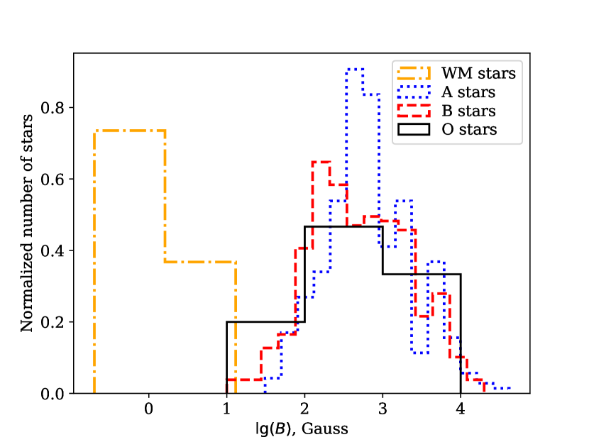
Figure 1: The histogram of magnetic field strengths for O, B, A and weakly magnetic (WM) stars in our sample. The upper limit of the magnetic field of WM stars is 10 G.

Magnetic field measurements were compiled from various sources, see Table 1 for details. We select only newer measurements (starting from 2006) with a relative error of less than 0.5. In this work, we use the value of the root-mean-square (rms) magnetic field (Bohlender et al., 1993):

$$B=\sqrt{\frac{1}{n}\sum_{k=1}^{n}(B_{l}^{k})^{2}},$$ (1)

where ${B_{l}}$ is longitudinal magnetic field component, $n$ is number of field measurements. We choose ${B_{\mathrm{rms}}}$ for this work, because it weakly depends on rotational orientation and phase of the star. Based on statistical simulations by Kholtygin et al. (2010) it is known that the polar magnetic field ($B_{p}$) and the rms magnetic field $B_{\mathrm{rms}}$ are related as $B_{\mathrm{rms}}\approx 0.2B_{\mathrm{p}}$. Hereafter, ${B}$ means ${B_{\mathrm{rms}}}$ and the polar magnetic field is labelled with p. We compile a catalogue which is available in Appendix C. We divide stars into strongly and weakly magnetised based on a threshold value of rms magnetic field of 10 G.

We plot the distribution of magnetic fields for different classes of stars in Figure 1. The Kolmogorov-Smirnov test shows that magnetic fields of A and B stars are drawn from two different distributions ($D=0.21$, $p=2\times 10^{-2}$). At the same time, if we perform the Kolmogorov-Smirnov test for a sample of A stars divided into two equal parts, we obtain approximately the same distribution laws ($D=0.19$, $p=0.28$). Similarly for B stars ($D=0.15$, $p=0.63$). It is worth noticing that the KS test by construction does not deal with measurement uncertainties. Therefore, we perform maximum likelihood analysis to estimate parameters of the magnetic field distribution.

#	Source	Number of stars
1	Alecian et al. (2014)	2
2	Alecian et al. (2016)	1
3	Aurière et al. (2007)	24
4	Bagnulo et al. (2017)	5
5	Blazère et al. (2016a)	1
6	Blazère et al. (2016b)	2
7	Castro et al. (2015)	1
8	Chojnowski et al. (2019)	30
9	David-Uraz et al. (2020)	1
10	Folsom et al. (2018)	1
11	Fossati et al. (2015a)	1
12	Freyhammer et al. (2008)	15
13	Grunhut et al. (2013)	1
14	Grunhut et al. (2009)	1
15	Hubrig et al. (2014a)	3
16	Hubrig et al. (2018)	1
17	Kobzar et al. (2020)	1
18	Kochukhov et al. (2018)	1
19	Kochukhov et al. (2019)	1
20	Kurtz et al. (2008)	1
21	Landstreet et al. (2008)	8
22	Ligniéres et al. (2009)	1
23	Mathys (2017)	17
24	Neiner & Lampens (2015)	1
25	Neiner et al. (2017b)	1
26	Petit et al. (2011)	1
27	Romanyuk et al. (2018a)	9
28	Shultz et al. (2018)	51
29	Shultz & Wade (2017)	1
30	Shultz et al. (2019b)	1
31	Shultz et al. (2020b)	2
32	Sikora et al. (2019)	14
33	Sikora et al. (2016)	1
34	Silvester et al. (2012)	2
35	Wade et al. (2015)	1
36	Wade et al. (2012a)	1
37	Wade et al. (2012b)	1
38	Wade et al. (2011)	1
39	Wade et al. (2006)	1
	Total	208

Table 1: Literature references for a compiled list of measurements of magnetic fields of massive stars

2.2 Maximum likelihood estimate

The maximum likelihood technique must be used to estimate parameters of the magnetic field distribution instead of the simple least-square used in previous works (see e.g. Igoshev & Kholtygin 2011) because the latter centres errors on the measured value, while in reality the errors are centred at the actual (unknown) value. As the initial distribution for magnetic fields, we choose the log-normal distribution with mean $\mu_{B}$ and standard deviation $\sigma_{B}$:

$$f(B|\mu_{B},\sigma_{B})=\frac{1}{B\log 10\sqrt{2\pi}\sigma_{B}}\exp\left(-\frac{(\log_{10}B-\mu_{B})^{2}}{2\sigma_{B}^{2}}\right),$$ (2)

where $\mathrm{\mu_{B}}$ is $\mathrm{\log_{10}B_{rms}}$ in Gauss and should be distinguished from $\mathrm{B_{p}}$.

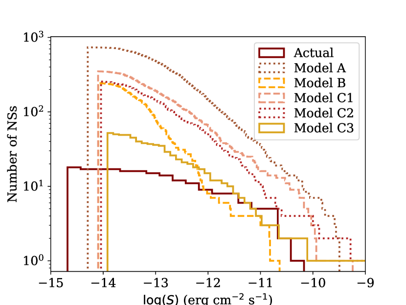
Figure 10: Cumulative distribution function for X-ray fluxes for magnetars. Maroon line is real observations from Mong & Ng (2018), see Table 3 for details of each model. X-ray luminosities decay only due to decay of surface dipolar poloidal magnetic field, see Section 3.3.1 for details.

The actual magnetic field $B$ is measured as $B^{\prime}$ because of the measurement process uncertainty. We assume that the distribution of $B^{\prime}$ as a function of $B$ follows the normal distribution, see e.g. figure 10 by Hubrig et al. (2014a). Therefore the conditional probability which describes the measurement process is written as:

$$p(B_{i}^{\prime}|B)=\frac{1}{\sqrt{2\pi}\sigma_{i}}\exp\left(-\frac{(B-B_{i}^{\prime})^{2}}{2\sigma_{i}^{2}}\right).$$ (3)

Here $\sigma_{i}$ is an error of magnetic field measurement for a particular star and should not be mixed with $\sigma_{B}$ which is a single unique value describing the distribution for the whole sample. The joint probability is a multiplication of probabilities eqs. (2) and (3). Because we do not know the value of the actual magnetic field, we integrate it out:

$$p(B_{i}^{\prime}|\mu_{B},\sigma_{B})=\frac{1}{2\pi\sigma_{B}\sigma_{i}\log 10}\int_{B_{\mathrm{min}}}^{B_{\mathrm{max}}}\frac{1}{B}\hskip 99.58464pt$$

$$\hskip 56.9055pt\times\exp\left(-\frac{(\log_{10}B-\mu_{B})^{2}}{2\sigma_{B}^{2}}-\frac{(B-B_{i}^{\prime})^{2}}{2\sigma_{i}^{2}}\right)dB.$$ (4)

This integral is computed numerically using the grid method with constant logarithmic step because the magnetic field ranges from a fraction of G to tens of kG. The log-likelihood function is written as:

$$\log\mathcal{L}(\mu_{B},\sigma_{B})=\sum_{i=1}^{N}\log(p(B_{i}^{\prime}|\mu_{B},\sigma_{B})).$$ (5)

We find the minimum of this function i.e. the maximum of the likelihood.

2.3 Result

We summarise the results of the maximum likelihood analysis in Table 2 and show the contours of confidence intervals in Figures 2,3 and Figure 4. Please note that the number of stars in Table 2 does not match the number of stars in the complete catalogue (see Table 1), because we selected only those values which satisfy the criterion: >$\mathrm{1.5\sigma}$. For stars of the spectral type B, the log-normal distribution is a suitable model. After the maximum likelihood optimisation we perform the Kolmogorov-Smirnov test and find the value of $D=0.08$ which corresponds to a p-value of 0.67. Therefore, no significant deviations from log-normality are present. For A stars the log-normal distribution seems to be marginally consistent with observations: it is worth noticing a large discrepancy between the analytic cumulative distribution and actual distribution of measured magnetic fields in Figure 3 around values of 2-3 kG. The Kolmogorov-Smirnov test which we perform after the optimisation gives $D=0.14$ which corresponds to a p-value of 0.035. It might be related to a fact that some low-mass A stars might have dynamo (Featherstone et al., 2009; Thomson-Paressant et al., 2021; Seach et al., 2020; Zwintz et al., 2020).

In Table 2 we analyse weakly magnetised stars separately. The reason to separate them is as follows: stars with a magnetic field of the order of 1 kG constitute 5-10 percent of the massive stellar population. These magnetic fields are easy to measure. Weaker magnetic fields are intrinsically challenging to discover in massive stars due to a limited number of observed absorption lines (Neiner & Lèbre, 2014). If weakly magnetised stars were an extended tail of the log-normal distribution seen in massive stars, we would expect magnetic fields of order 1 G to be found in less than $2.82/0.65\approx 4.4\sigma$ cases i.e. in less than 1 in 15000 cases per one strongly magnetised star. In reality, we have 9 measurements (4 good quality for main sequence stars) per 92 strongly magnetised stars and many more are expected to be found with an improvement of instrumentation. Therefore, it is quite safe to assume that a large number (comparable to 50-90 percent of all massive stars) might have weak surface magnetic fields that are hard to measure. We characterise them using an available sample of weakly magnetised stars even though this sample is small and incomplete. We should be cautious and remember that there are stars with non-detected magnetic fields even despite a very low detection threshold, see Neiner et al. (2014).

Spectral type	N	$\mu_{B}$	$\sigma_{B}$	$-2\log\mathcal{L}^{*}$
		$\log_{10}\mathrm{[G]}$
O	10	$2.62\pm 0.16$	$0.26^{+0.24}_{-0.11}$	137
B	91	$2.82\pm 0.10$	$0.65\pm 0.09$	1416
A	93	$3.06\pm 0.11$	$0.66\pm 0.07$	3414
Weak magnetic	4	$0.14\pm 0.5$	$0.7_{-0.27}^{+0.57}$	15

Table 2: Result of the maximum likelihood analysis. N is number of stars of particular spectral type. Uncertainties are 70 per cent confidence intervals. We selected only measurements which are $>1.5\sigma$.

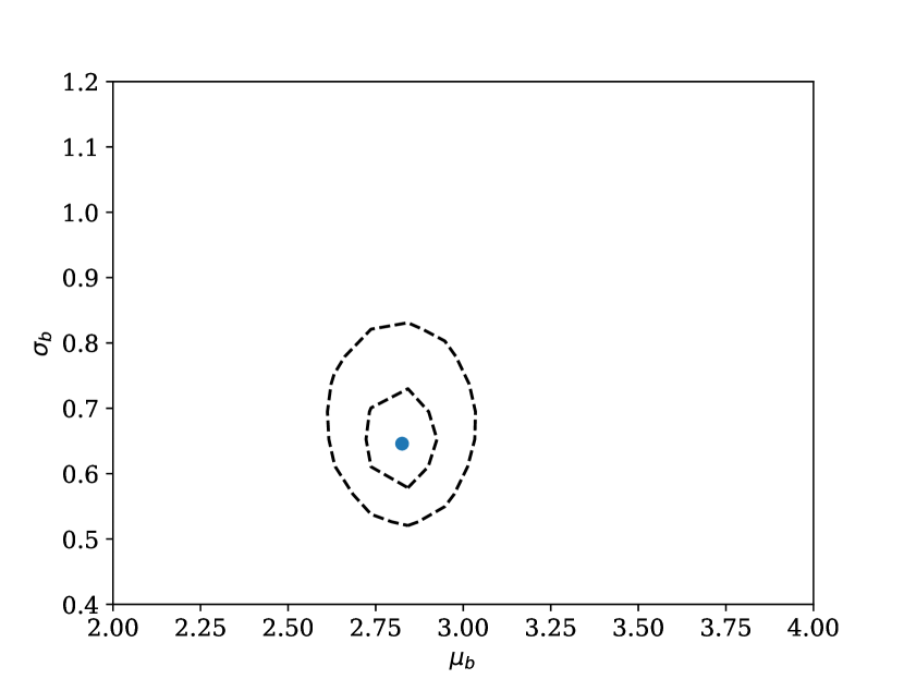
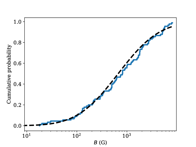
Figure 2: The position of the maximum likelihood (dot) and credible intervals (70 percent and 99 percent) for parameters of the log-normal distribution for B spectral type stars (left panel). We show the cumulative probability for measured magnetic fields for B stars using a blue solid line and cumulative probability for the best model using a dashed black line.

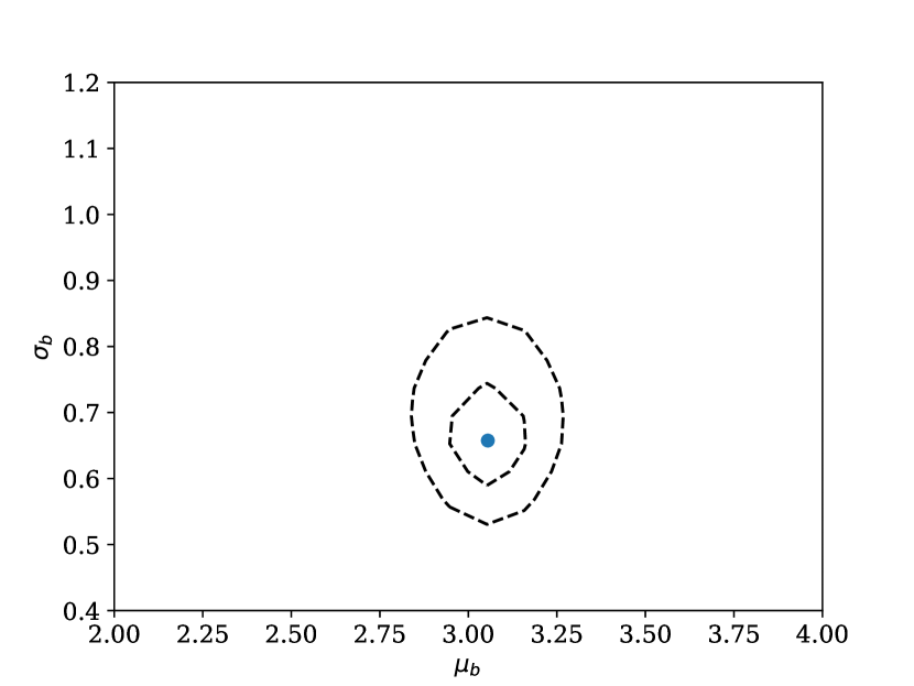
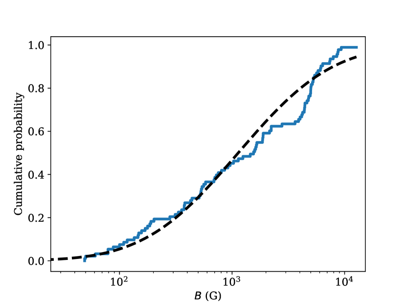
Figure 3: The same as Fig. 2, but for A stars.

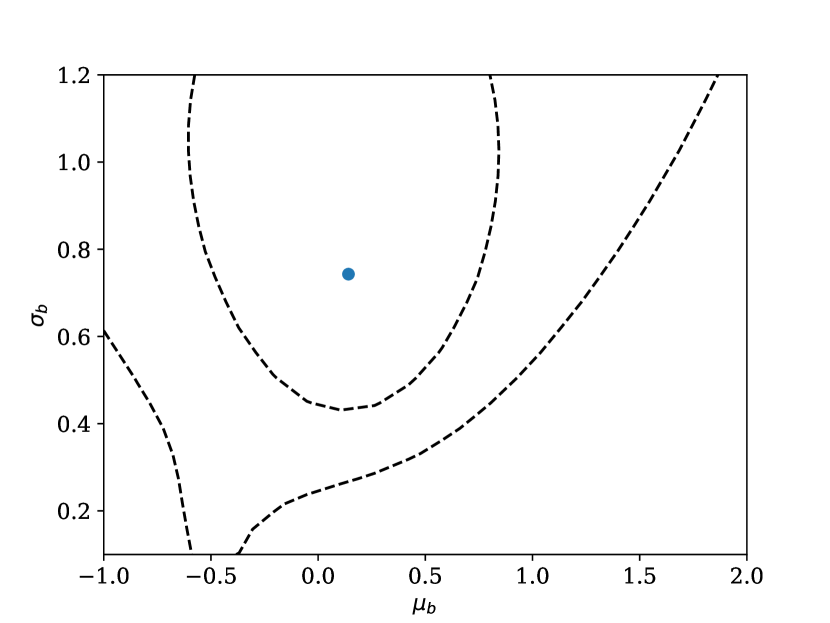
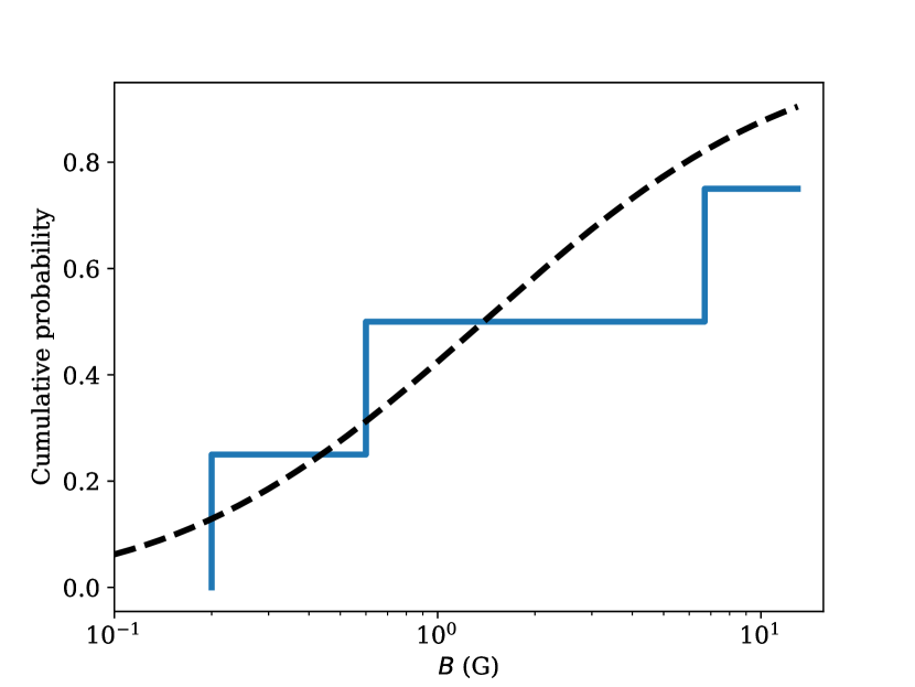
Figure 4: The same as Fig. 2, but for weakly magnetised stars.

It is interesting to note that the standard deviation of the log-normal distribution for B stars is $0.65\pm 0.09$ which is within 1-sigma interval of standard deviation independently derived for radio pulsars $\sigma_{\log B}=0.55$ (Faucher-Giguère & Kaspi, 2006). As for the shift of distribution following argument applies: if we assume that $\log_{10}B=2.62$ is representative of a magnetic field for a typical B2V with the radius of $5.3R_{\odot}$ and during a collapse, radius shrinks to 10 km, the magnetic field could be amplified many orders of magnitude and reach $\mu_{B}\approx 14$ which is typical for magnetars. We discuss this possibility in more details in Section 3.2.1. It is worth to note that magnetic field might decay during the lifetime of massive star. Such possibility was discussed by Shultz et al. (2019a). Medvedev et al. (2017) tried to estimate the magnetic field decay timescale and found that it exceeds the half of main sequence lift-time. Therefore, we do not expect a very strong decay before NS formation.

3 Magnetic Neutron stars

3.1 Data

In order to compare the results of our analysis with real pulsars and magnetars we use the ATNF catalogue (Manchester et al., 2005), McGill Online magnetar catalogue (Olausen & Kaspi, 2014) and Magnetar Outburst Online Catalog (Coti Zelati et al., 2018). For detailed comparison of X-ray fluxes we use data by Mong & Ng (2018) and Viganò et al. (2013) derived for X-ray energy range 2-10 keV and 1-10 keV respectively.

3.2 Population synthesis of massive stars and NSs

In this research, we use the population synthesis code NINA (Nova Investigii Neutronicorum Astrorum sentence in Latin standing for New Study of Neutron Stars). The simulation algorithm is mostly similar to one presented by Faucher-Giguère & Kaspi (2006) with a few small changes.

We draw masses and positions of massive stars instead of positions of NS. We fix the birthrate at the level of $n_{\mathrm{br}}=7$ stars in mass range 8-45 $M_{\odot}$ per thousand years. Therefore, we draw 7 stars every thousand years adding a random shift to their birth time to spread them uniformly inside the thousand years interval. Masses of stars are drawn from the Salpeter (1955) initial mass function. We draw positions equally probably from one of four spiral arms, using the same parameters are Faucher-Giguère & Kaspi (2006). The initial metallicity of a star depends on its birth-location according to Maciel & Costa (2009). The spiral pattern rotates with speed 26 km s^-1 kpc^-1 (Dias & Lépine, 2005; Gerhard, 2011). Peculiar velocities of massive stars are drawn from Maxwellian with $\sigma=15$ km s^-1.

Further, we compute lifetime on the main sequence, core mass at the end of evolution and radius of the star using equations derived by Hurley et al. (2000). The mass and position for NSs are computed based on the parameters of massive stars. The natal kick of NSs is drawn from the sum of two Maxwellians distribution according to Verbunt et al. (2017); Igoshev (2020) in a form:

$$f(v)=w\sqrt{\frac{2}{\pi}}\frac{v^{2}}{\sigma_{1}^{3}}\exp\left(-\frac{v^{2}}{2\sigma_{1}^{2}}\right)+(1-w)\sqrt{\frac{2}{\pi}}\frac{v^{2}}{\sigma_{2}^{3}}\exp\left(-\frac{v^{2}}{2\sigma_{2}^{2}}\right),$$ (6)

with uniform distribution of the natal kick orientation on a sphere. We use parameters $w=0.42$, $\sigma_{1}=75$ km s^-1 and $\sigma_{2}=316$ km s^-1.

We integrate the motion of NSs in the Galactic gravitational potential (Kuijken & Gilmore, 1989) using the fourth-order Runge-Kutta method. We assume that the magnetic field of normal radio pulsars does not decay based on recent research (Igoshev, 2019). For magnetar candidates ($B>10^{13}$ G and age less than 1 Myr) we post-process result and model magnetic field decay using the same scheme as was described in works by Igoshev & Popov (2018, 2015). This modelling includes the inner crust impurity parameter $Q$ which determines the magnetic field decay timescale due to Ohmic losses. It is believed that impurity parameter is large $Q\gg 1$ (Pons et al., 2013) for magnetars since it provides a convenient explanation for the absence of magnetars with a period longer than 12 sec.

We compute radio luminosity of pulsars using the same technique as described by Faucher-Giguère & Kaspi (2006) and we implement exactly the same conditions for the pulsar detectability. The dispersion measure is calculated using the source code by Yao et al. (2017). For the sky map temperature at radio frequency 1.4 GHz we use map by Dinnat et al. (2010).

To compare the population of synthetic radio pulsars with observations we bin the $P$ – $\dot{P}$ into 20 rectangular areas and compute the C-statistics for each individual bin, see Appendix A for details. The advantage of C-statistics in comparison to 2D KS test used by Gullón et al. (2015) is that it is more sensitive to bins with a small number of pulsars. The use of C-statistics is also better justified because the drawing process for pulsars in the particular bin should follow the Poisson distribution. Based on the comparison between $P$ – $\dot{P}$ of the Parkes and Swinburne surveys with the modern ATNF data, we conclude that C-statistics difference up to 8-12 means that we can reproduce the sample of observed radio pulsars.

3.2.1 Magnetic fields of NSs in the case of fossil origin

The configuration of the magnetic field inside a massive star is complicated. A stable configuration most probably includes both poloidal and toroidal components (Braithwaite & Nordlund, 2006). Here we simplify it significantly to consider only extreme cases. More detailed analysis requires numerically expensive magnetohydrodinamical modelling. We choose two limiting scenarios: (1) only the core of the star is a good conductor, so currents flow only there (see right panel of the Figure 5) and (2) whole star is a uniformly conducting body (left panel of the same figure).

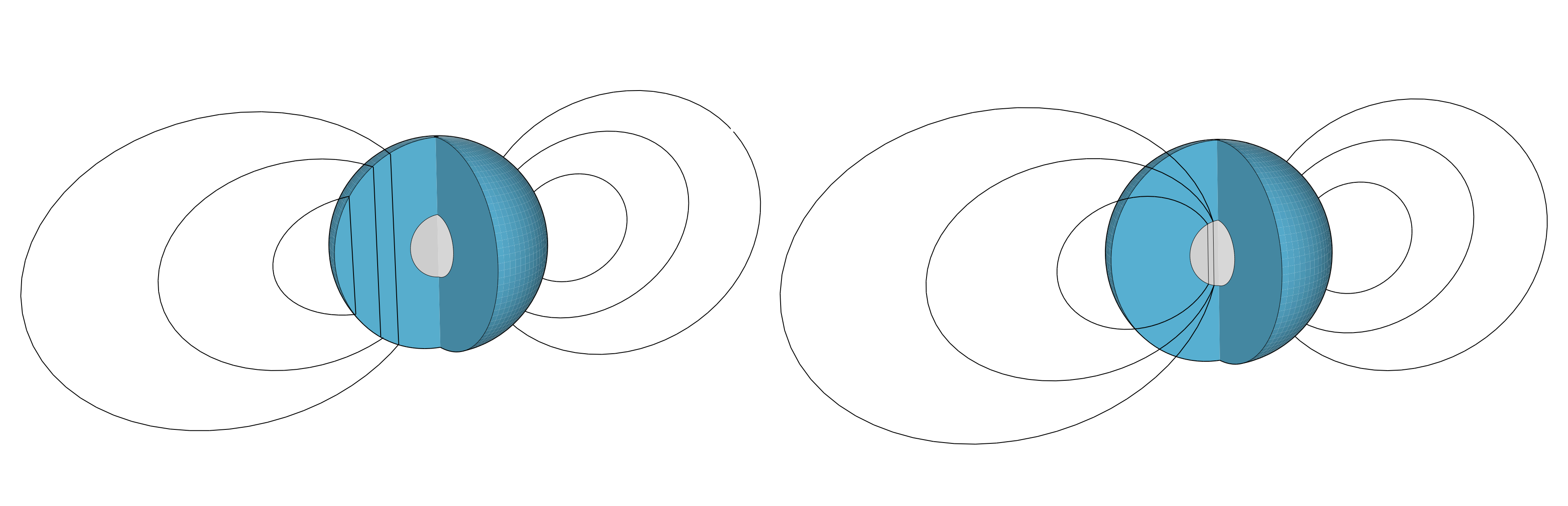
Figure 5: Schematic view of magnetic field lines inside and outside of a massive star. The blue region is a radiative envelope, the grey region is a convective core and solid lines show the magnetic field lines.

Magnetic flux conservation

In earlier works, e.g. Igoshev & Kholtygin (2011) researchers considered a conservation of magnetic flux defined as $F=4\pi B_{\mathrm{pole}}R_{*}^{2}$ where $R_{*}$ is the stellar radius and $B_{\mathrm{pole}}$ is the magnetic field at the pole. Kholtygin et al. (2010) noticed that the magnetic field at the pole of a massive star is $\alpha\approx 5$ times stronger than the rms field measured based on spectral lines. In studies of radio pulsars, researchers commonly use magnetic field strength at NS equator (Lorimer & Kramer, 2004) which is two times smaller than the field at the pole for dipolar configuration. Therefore, we use a coefficient $\alpha/2$.

After the supernova explosion, NS has a radius of $R_{\mathrm{ns}}\approx 10$ km which means that its magnetic field is:

$$B^{\mathrm{NS}}=\frac{\alpha}{2}B_{\mathrm{rms}}\left(\frac{R_{*}}{R_{\mathrm{ns}}}\right)^{2}.$$ (7)

Here we consider an example O star with $R_{*}=10$ R_⊙. If this star is strongly magnetised it can produce NS with mean $B^{\mathrm{NS}}_{p}=5\cdot 10^{14}$ G. If this star is weakly magnetised, it produces an NS with mean $B^{\mathrm{NS}}=1.7\cdot 10^{12}$ G. We use these parameters in our model D for $\mu_{B}$. On the other hand, if we consider a B star (B2V, R = 5 R_⊙), we obtain: $B^{\mathrm{NS}}=2\cdot 10^{14}$ G and $B^{\mathrm{NS}}=4.2\cdot 10^{11}$ G.

Core conductivity

We assume that the general configuration of magnetic field is a dipole (see Figure 5, right panel). In this case, the magnetic field at the pole of a core is stronger than the magnetic field at the pole of a massive star:

$$B_{\mathrm{core,pole}}=2B_{\mathrm{p}}\left(\frac{R_{*}}{R_{\mathrm{core}}}\right)^{3}.$$ (8)

In this case the NS magnetic field at equator is:

$$B^{\mathrm{NS}}=B_{\mathrm{p}}\left(\frac{R_{*}}{R_{\mathrm{core}}}\right)^{3}\left(\frac{R_{\mathrm{core}}}{R_{\mathrm{ns}}}\right)^{2}.$$ (9)

We take two typical B-stars (B2V, $R_{*}$ = 5 R_⊙, $R_{\mathrm{core}}=0.3R_{*}$ D. Szécsi, 2020, private communication) : (1) strongly magnetic with $B_{\mathrm{star}}\approx$ 700 G and (2) weakly magnetic with $B_{\mathrm{star}}$ $\approx$ 1.4 G and calculate the magnetic field expected at the NS stage as B${}^{\mathrm{NS}}\approx 5\cdot 10^{11}$ G and B${}^{\mathrm{NS}}\approx 2.8\cdot 10^{14}$ G. These values are nearly identical to ones we obtain for B star in an assumption of magnetic flux conservation. These magnetic fields could correspond to normal radio pulsars and magnetars. So, we proceed with this model further and show results of the population synthesis in Section 4, model E.

Uniformly conducting star

In this case the magnetic field lines inside the star are straight (see Figure 5, left panel). The magnetic field of the core is a fraction of the surface magnetic field strength which is proportional to the fraction of volume of the core to the volume of the star. The magnetic field at the core can be computed as:

$$B_{\mathrm{core,pole}}=2B_{\mathrm{p}}\left(\frac{R_{\mathrm{core}}}{R_{*}}\right)^{3}.$$ (10)

In this case the NS magnetic field at equator is:

$$B^{\mathrm{NS}}=B_{\mathrm{p}}\left(\frac{R_{\mathrm{core}}}{R_{*}}\right)^{3}\left(\frac{R_{\mathrm{core}}}{R_{\mathrm{ns}}}\right)^{2}.$$ (11)

In reality the radiative envelope is less dense than the core and is consequently less conductive. Additional toroidal magnetic field makes the situation even more complicated.

Again, if we take two typical B-stars and calculate the magnetic field for NSs, we get $B^{\mathrm{NS}}$ $\approx$ $4\cdot 10^{8}$ G, $B^{\mathrm{NS}}$ $\approx$ $2\cdot 10^{11}$ G. We can immediately conclude that this scenario is extremely unrealistic, since the resulting average magnetic fields of NSs are several orders of magnitude lower than the real ones. Therefore, we do not consider this model anymore.

3.3 Population synthesis of magnetars

The observational selection for magnetars is very different from one for normal radio pulsars, see e.g. Gullón et al. (2015). Magnetars are often discovered during outbursts in X-rays and $\gamma$-rays and confirmed later on by follow up observations aimed at the determination of the rotational period and period derivative. Unlike pulsars, magnetars often do not emit radio and follow up observations happen in X-rays to characterise the quiescence state. Therefore, the absorbed X-ray flux in quiescence is the main observational limitation.

The X-ray flux in quiescence depends on magnetic fields which is not constant. The magnetars are believed to lose a significant part of their magnetic energy in $\approx 1$ Myr (Pons et al., 2013; Igoshev & Popov, 2018).

We perform population synthesis as following: first, we introduce a toy model for magnetar population synthesis to illustrate different factors that play an essential role in the population synthesis, and then in Section 3.3.2 we compute a more realistic model.

3.3.1 Toy models for X-ray luminosity

We use a toy model to illustrate the importance of X-ray luminosity for the population synthesis of magnetars. In this toy model we assume no magnetic field decay and choose an initial distribution for magnetic fields in form similar to Faucher-Giguère & Kaspi (2006) i.e. $\mu_{B}=12.65$ and $\sigma_{B}=0.5$. From the results of pulsar population synthesis we select objects with $B_{0}>10^{13}$ G and age $<10^{6}$ years. A similar complete model was computed by Gullón et al. (2015) as model A.

Observed X-ray flux of magnetars is affected by complicated energy redistribution in the X-ray spectra and absorption in the Galaxy. We keep details of this process until Section 3.3.4, but here we consider the dependence of luminosity $L_{X}$ and flux $S_{X}$ on the initial magnetic field and age of the magnetar. Because we do not have access to results of detailed magneto-thermal NS evolution with cooling, we use an empirical model which we calibrate using magnetar observations and figure 11 in Viganò et al. (2013). We recommend future researchers who simulate the cooling of magnetars to make the results of their work publicly available to simplify magnetar population synthesis.

We study evolution of luminosity in the form: $L_{X}(B_{0},t)=L_{1}(B_{0})L_{2}(t)$. According to figure 11 in Viganò et al. (2013) the temperature evolves first as power-law of time and start decaying exponentially at timescales of $\propto 10^{5}$ years. So, in the first toy model we assume the initial temperature $T_{0}=0.4$ keV = $4.6\times 10^{6}$ K. We further describe the evolution of luminosity as:

$$L(t)=4\pi R^{2}\sigma T_{0}^{4}\left(\frac{t}{1\;\mathrm{year}}\right)^{-0.26}\exp\left(-\frac{t}{10^{5}\;\mathrm{years}}\right).$$ (12)

We plot the evolution of luminosity for this model in Figure 6. It is immediately obvious that despite quite a large initial temperature, the model misses some magnetars. There is an intrinsic spread in X-ray luminosities seen for magnetars of similar age.

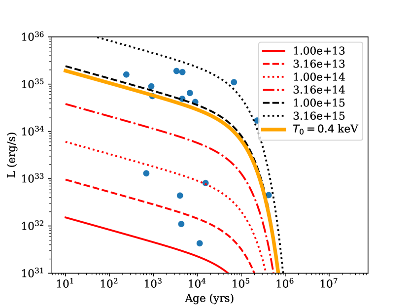
Figure 6: X-ray luminosity as a function of time and initial magnetic field in Gauss. The legend shows the values of the initial magnetic field in Gauss. Blue dots show luminosities derived for magnetars in the McGill catalogue.

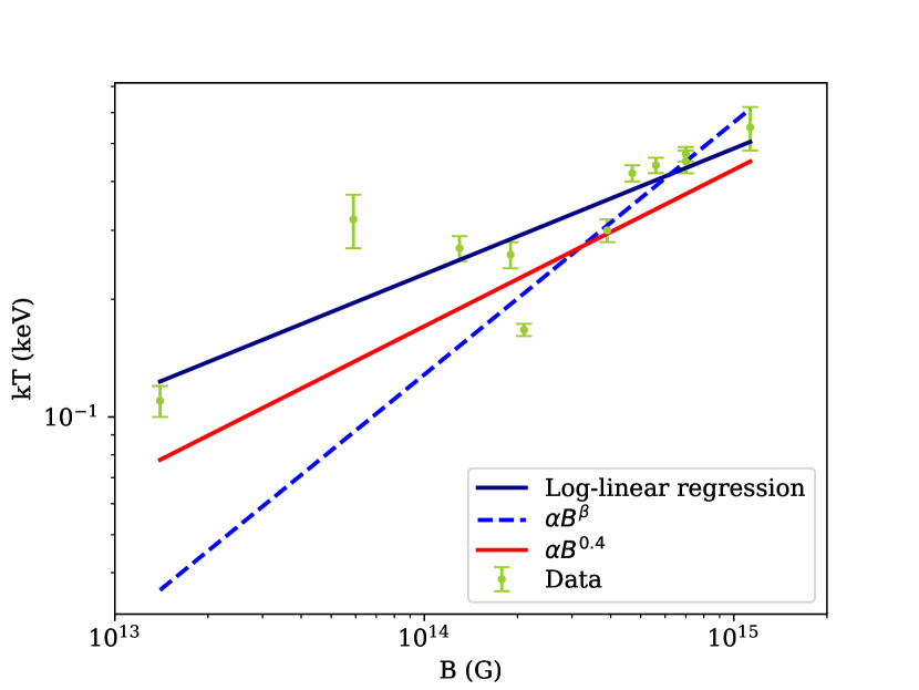
Figure 7: The $kT-B$ dependence for real observed magnetars. Different models of approximation are described in the legend of the graph. The axes are logarithmic.

Further we look at the observational dependence between bulk temperature and magnetic field. We use a fit for surface temperatures similar to work by Mong & Ng (2018); Coti Zelati et al. (2018):

$$T\propto\alpha B^{0.4},$$ (13)

where $T$ stands for surface temperature of the magnetar, $B$ is the initial magnetic field. Using the data collected in the article Mong & Ng (2018) for 11 observed magnetars in the quiescent state, we obtain an approximation:

$$T=4.3\times 10^{-7}\left(\frac{B_{0}}{1\;\mathrm{G}}\right)^{0.4}\;\mathrm{keV}.$$ (14)

This approximation is shown in Figure 7. Then we use this dependence for temperature and compute luminosity and flux as:

$$L=4\pi R^{2}\sigma T^{4}\;\hskip 28.45274pt\;\;S=\frac{L}{4\pi D^{2}},$$ (15)

where $D$ is the distance of the magnetar from Earth. We obtain this parameter from the pulsar population synthesis. In this model we overproduce bright X-ray sources, see Figure 8 for toy population synthesis and Figure 10 for more realistic population synthesis when we take fast magnetic field decay into account. The brightest sources produced in model A should be limited by $S\approx 10^{-12}$ erg cm^-2 s^-1. In our model we get plenty of sources with fluxes $10^{-10}$ – $10^{-11}$ erg cm^-2 s^-1. It is also interesting to note that if we introduce a magnetic field decay and substitute the instant value of the magnetic field in eq. (14) it is possible to reproduce decay in luminosity. However, in this case, the luminosity distribution starts depending on the timescale of magnetic field decay (and impurity parameter $Q$ respectively) which is not seen in models produced by Gullón et al. (2015). Instead, their models for different time scales of magnetic field decay produce flux distributions that are basically identical.

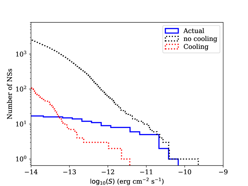
Figure 8: X-ray fluxes of magnetars obtained in two toy models. The solid blue line corresponds to the distribution of X-ray fluxes of magnetars in quiescence from the McGill catalogue. THe dotted red line shows X-ray fluxes seen in a model with exponential decay of luminosity with time. The dotted black line shows X-ray fluxes seen in a model where the luminosity decay only due to decay of the magnetic field.

Therefore a realistic model for luminosity should include both components: (1) spread in initial temperatures as a function of the initial magnetic field and (2) cooling. Our combined model is:

$$L(t)=2.5\times 10^{3}\pi R^{2}\sigma\left(\frac{B_{0}}{1\;\mathrm{G}}\right)^{1.6}\left(\frac{t}{1\;\mathrm{year}}\right)^{-0.26}\hskip 56.9055pt$$

$$\hskip 142.26378pt\times\exp\left(-\frac{t}{10^{5}\;\mathrm{years}}\right)\;\mathrm{egs/s}.$$ (16)

The luminosity evolution for different values of the initial magnetic field for this model is shown in Figure 6. We see that different tracks enclose all observed magnetars. We substitute this model in our toy population synthesis and show results in Figure 8. As it is expected model with cooling lies well below the actual magnetars which is in agreement with curve for model A in Gullón et al. (2015). We do not overproduce bright sources anymore. Further, we use this luminosity model as a basic model in our advanced population synthesis.

The parameters which we selected in eq. (16) are not arbitrary. The value of the exponent is restricted on one hand by a necessity to include the brightest magnetars (e.g. a value of $-0.5$ does not work already) and to have some luminosity decline compatible with simulations, see figure 11 in Viganò et al. (2013). The time scale for luminosity decay cannot be any shorter (we miss magnetars) and cannot be significantly longer (we overproduce bright sources).

3.3.2 Advanced magnetar population synthesis

The magnetar population synthesis proceeds in the following steps: (1) we select from the results of pulsar population synthesis NSs with ages $T<1\times 10^{6}$ years, with initial magnetic fields above $10^{13}$ G. In this selection we include objects independently of how probable it is to detect them in a pulsar radio survey; (2) we compute their magnetic fields at the current moment taking into account the impurity parameter $Q$; (3) we compute their expected temperature as a function of their initial magnetic field and (4) we model their X-ray spectra and fluxes taking absorption and distance into account. In the end, we compare the cumulative distribution for X-ray fluxes and final spin periods.

3.3.3 Magnetic field decay

We use the phenomenological model described in Igoshev & Popov (2015, 2018, 2020b, 2020a). Namely, we integrate numerically an approximate differential equation by Aguilera et al. (2008):

$$\frac{dB_{p}}{dt}=-\frac{B_{p}}{\tau_{\mathrm{Ohm}}(T_{\mathrm{crust}})}-\frac{1}{B_{0}}\frac{B_{p}^{2}}{\tau_{\mathrm{Hall}}},$$ (17)

where $B_{p}$ is the poloidal, dipolar magnetic field at the NS pole, $B_{0}$ is the initial poloidal dipolar field strength, $\tau_{\mathrm{Hall}}$ is the initial Hall timescale and $\tau_{\mathrm{Ohm}}$ is the Ohmic timescale for the temperature of the deep NS crust $T_{\mathrm{crust}}$. One of the main factors which govern the magnetic field evolution for magnetars is their crust impurity. We relate the timescale for magnetic field decay with a value of the impurity parameter as:

$$\tau_{Q}=\frac{2\;\mathrm{Myr}}{Q},$$ (18)

which roughly corresponds to the case when most of the current flow at densities $\approx 5\times 10^{13}$ g cm^-3. Based on magnetic field decay curve figure 2 by Gullón et al. (2014) we see that their relationship between time scale and $Q$ is:

$$\tau_{Q}\approx\frac{20\;\mathrm{Myr}}{Q},$$ (19)

because they assume that most of the current flows at densities $\approx 5\times 10^{14}$ g cm^-3. Therefore their $Q=100$ roughly corresponds to our $Q=10$ and their $Q=25$ would correspond to our $Q=2.5$. This difference is simply related to a different choice of parameters and can be easily re-scaled in our model if new observations prove that our choice is nonphysical.

We show our magnetic field decay curves in Figure 9. As it was discussed in Section 3.3.1, the magnetic field decay law does not affect the X-ray flux, so it affects only the distribution of observed periods.

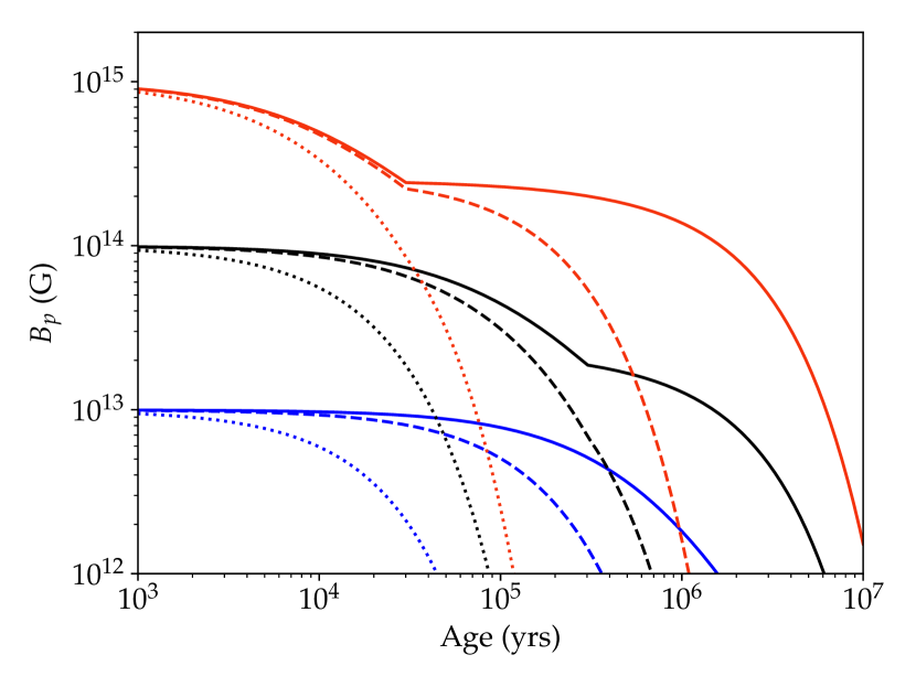
Figure 9: Strength of the poloidal dipolar magnetic field as a function of time and impurity parameter $Q$. Solid lines correspond to $Q=1$, dashed lines to $Q=10$ and dotted lines to $Q=100$.

3.3.4 Modelling spectra and observational X-ray fluxes

Observations of magnetars in the quiescent state showed that their spectra consist both of thermal blackbody emission and non-thermal power-law tail at higher energies. We use the model by Lyutikov & Gavriil (2006) to take into account the scattering of thermal photons on the electrons of the magnetosphere. It is parameterized by two quantities: the optical depth $\tau_{\mathrm{res}}$ (which is related to the plasma density) and the thermal velocity of electrons in units of the speed of light $\beta_{\mathrm{T}}$. The corrected formulas of the reflected and transmitted flux are given in Appendix B.

Further, we correct these spectra for interstellar absorption. For the case of interstellar absorption an effective model of resonant Compton scattering could improve the number of detectable NSs, because the Compton scattering shifts low-energy photons to higher energies, so they can avoid absorption.

To account for absorption we use the Leiden/Argentine/Bonn (LAB) Survey of Galactic HI sky Kalberla et al. (2005). The final spectrum is then (Potekhin et al., 2016):

$$F_{\mathrm{fin}}=F(\omega)\cdot\exp\left[-\left(\frac{N_{H}}{10^{21}\mathrm{cm^{-2}}}\right)\cdot\left(\frac{h\omega}{2\pi\;0.16\;\mathrm{keV}}\right)^{-8/3}\right],$$ (20)

for each step of energy in the range from $0.1$ to $10$ keV. Here $F(\omega)$ is the flux before absorption, $N_{H}$ is the hydrogen density column in the direction of the magnetar, $h$ is the Planck constant and $\omega$ is the radiation frequency.
By combining the spectrum with a map of Galactic hydrogen and normalising it, we compute how much of the radiation was absorbed (denote this value as $\eta$, $\mathrm{\eta}\geq$ 1).

$$\eta=\frac{\int F_{\mathrm{fin}}(\omega)d\omega}{\int F_{\mathrm{bb}}(\omega)d\omega}.$$ (21)

Where we integrate from 0.1 keV to 10 keV. As a result we compute the received X-ray flux as:

$$S=\frac{L_{\mathrm{bol}}}{4\pi D^{2}}\cdot\mathrm{\eta}.$$ (22)

We assume that the thermal radiation from magnetars is not beamed.

4 Results

We summarise the results of our runs in Table 3. We also plot the cumulative distribution of X-ray fluxes in Figure 11 and 12. We notice that our run with initial parameters similar to Faucher-Giguère & Kaspi (2006) reproduces well the population of isolated radio pulsars as it is expected, see results for model B and Figure 14. This model does not describe the population of magnetars, because it does not produce enough stars with magnetic fields above $4\times 10^{13}$ G, so we see a lack of magnetars with observed X-ray fluxes in the range $10^{-10}$ – $10^{-12}$ erg cm^-1 s^-1, see Figure 11. This result is in agreement with Gullón et al. (2015). Model A with a slightly larger initial magnetic field overproduces the strongly magnetised radio pulsars, see Figure 14. This is why its C-statistics value is larger in comparison to model B.

Model	$w$	$\mu_{B,1}$	$\sigma_{B,1}$	$\mu_{B,2}$	$\sigma_{B,2}$	$Q$	C-stat	Comment
	%	$\log_{10}$ G		$\log_{10}$ G			per d.o.f
A	100	13.34	0.76			1	16.6	similar to Model B (Table 2) in Gullón et al. (2015)
B	100	12.65	0.55			1	7.89	similar to Faucher-Giguère & Kaspi (2006)
C1	70	12.59	0.59	13.33	0.83	1	6.61	similar to Model F (Table 3,4) in Gullón et al. (2015)
C2	70	12.59	0.59	13.33	0.83	10	6.61	similar to Model F (Table 3,4) in Gullón et al. (2015)
C3	70	12.59	0.59	13.33	0.83	100	6.61	similar to Model F (Table 3,4) in Gullón et al. (2015)
D	90	12.2	0.6	14.7	0.6	1	15.2	simple flux conservation eq.(7)
E	90	11.7	0.7	14.45	0.7	1	38.64	simple model for core conductivity eq.(9)
F1	90	12.65	0.7	15.35	0.7	1	7.59	fossil field hypothesis
F2	90	12.65	0.7	15.35	0.7	10	7.59	fossil field hypothesis
F3	90	12.65	0.7	15.35	0.7	100	7.59	fossil field hypothesis
F4	90	12.65	0.7	15.35	0.7	200	7.59	fossil field hypothesis

Table 3: Models calculated in our research and their results. C-stat value is divided by the total number of bins (20²). $w$ shows a fraction of objects drawn from the first component of bimodal log-normal distribution.

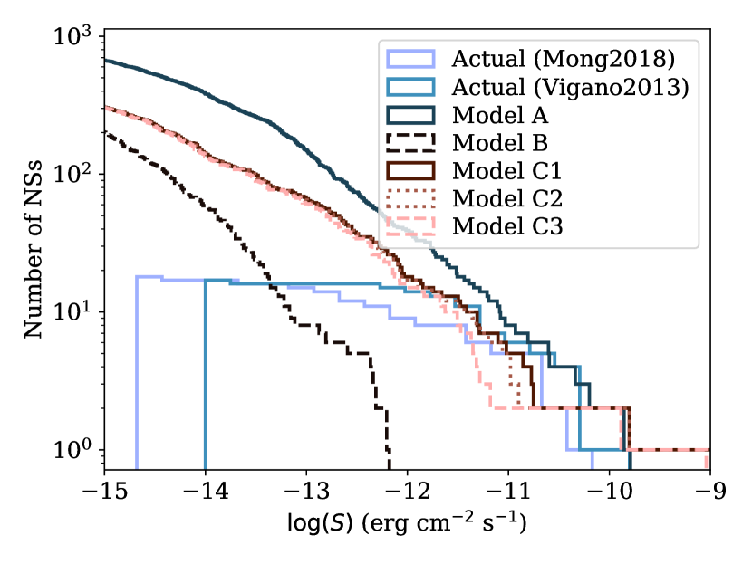
Figure 11: Cumulative distribution for X-ray fluxes of magnetars. Light blue line shows observations by Mong & Ng (2018); blue line shows observations by Viganò et al. (2013). See Table 3 for details of each model.

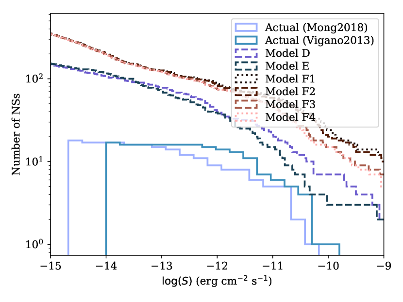
Figure 12: Cumulative distribution function for magnetars. Real observations are from Mong & Ng (2018), Model E is our approximation that initial magnetic filed should be two gaussians with weakly and stongly magnetic stars parameters, inherited from massive stars, see 3 for details of each model.

Models C1-C3 with initial parameters from Gullón et al. (2015) could reproduce the population of isolated radio pulsars quite well, see Figure 15. The value of C-stat per degree of freedom is even slightly smaller than in the case of the initial conditions similar to Faucher-Giguère & Kaspi (2006). As for the magnetars, all C models reproduce the observed X-ray fluxes well, see Figure 11, taking into account the fact that our current catalogue of magnetars is probably incomplete below fluxes $5\times 10^{-13}$ erg cm^-2 s^-1. A similar threshold value was also noted by Gullón et al. (2015). It is also interesting to note that if we select only magnetars with fluxes above this threshold, we closely reproduce the magnetar distance distribution, see Figure 13 (with exception of model A).

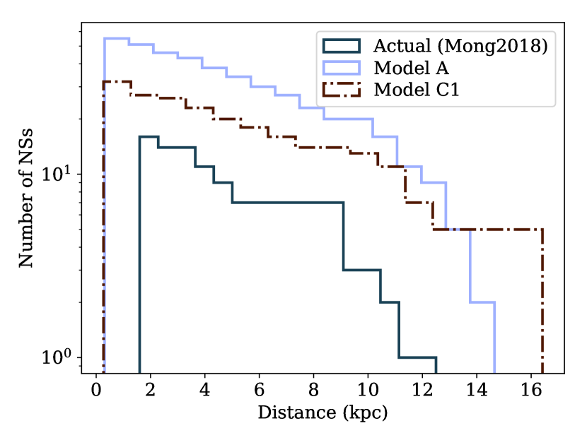
Figure 13: Cumulative distribution function for magnetars with fluxes $>5\cdot 10^{13}$ $\mathrm{ergcm^{-2}s^{-1}}$. See Table 3 for details about each model. Two magnetars are excluded from the actual sample (SGR 0526–66 in the LMC and CXOU J010043.1–721134 in the SMC), because we are considering only the galactic population.

As for observed period distribution, we would prefer impurity values between $10$ and $100$ because C2 overproduces magnetars with observed periods longer than 12 s and model C3 under-produces a total number of magnetars, see Figure 21 It is possible to find the exact value of the impurity parameter $Q\in[10,100]$ which describes the period distribution of magnetars.

To test the fossil field hypothesis, we first introduce model D where we compute the initial distribution of NS magnetic fields using simple flux conservation for O stars, see eq. (7). As it is seen from $P$ – $\dot{P}$ plot, Figure 16, the mean magnetic field $\mu_{B}=12.2$ is clearly small for normal radio pulsars. We produce too many weakly magnetised pulsars in this case. On the other hand, we produce too many bright magnetars (approximately 10) with $S_{X}$ in range $10^{-8}-10^{-10}$ erg cm^-2 s^-1, see Figure 12. Such magnetars are not observed.

Further, we introduce model E based on our simple estimates of magnetic field inherited to NS at the moment of a supernova explosion, described in Section 3.2.1. We notice that initial magnetic fields of radio pulsars produced in this model $\mu_{B}=11.7$ are smaller than typical for observations ($\mu_{B}=12.6$ in Faucher-Giguère & Kaspi 2006) by nearly an order of magnitude. The value of C-statistics and visual inspection of Figure 17 immediately show that the main pulsar cloud is significantly shifted toward small period derivative values. Therefore, we did not try to optimise this model by using different values of impurity parameter $Q$.

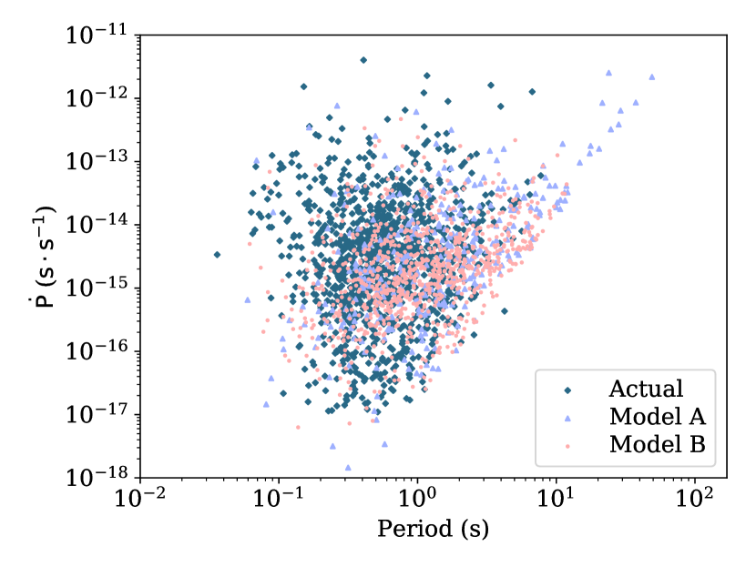
Figure 14: $P$ - $\dot{P}$ diagram for real pulsars and for Model A, B.

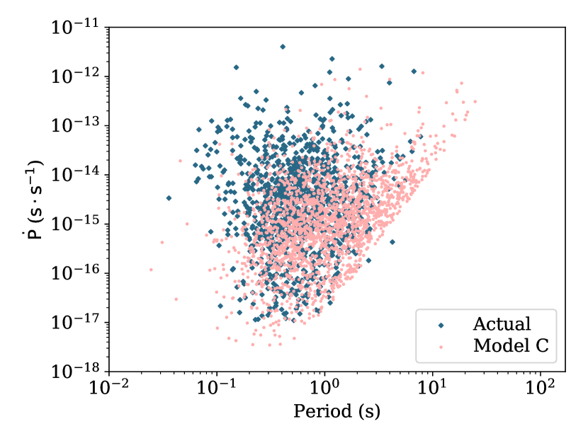
Figure 15: $P$ - $\dot{P}$ diagram for real pulsars and for Model C.

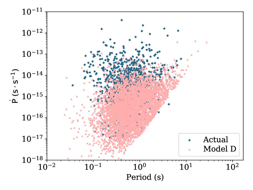
Figure 16: $P$ - $\dot{P}$ diagram for real pulsars and for Model D.

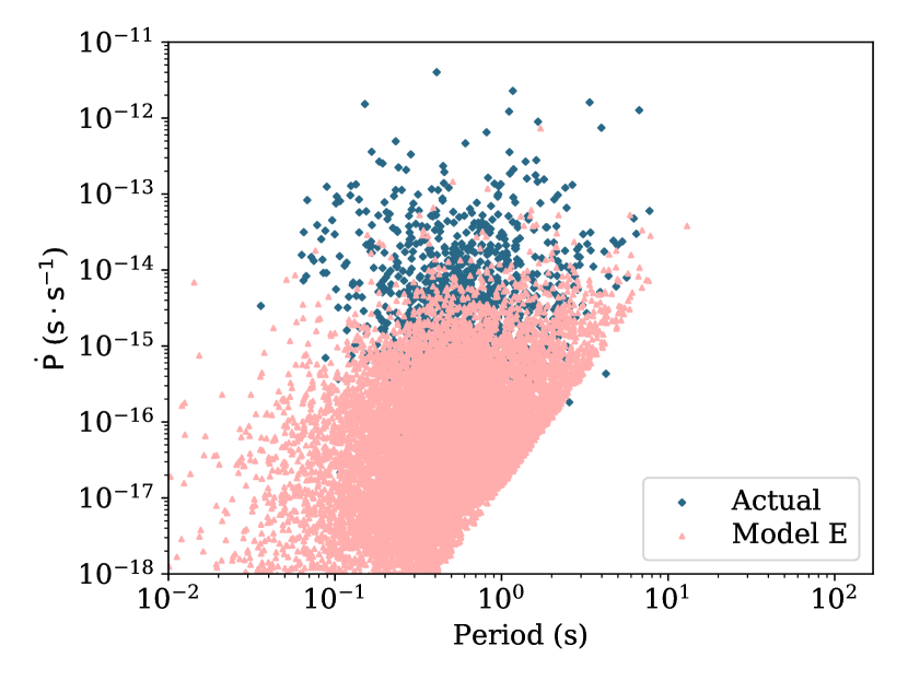
Figure 17: $P$ - $\dot{P}$ diagram for real pulsars and for Model E.

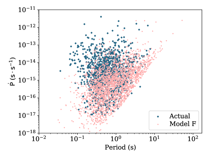
Figure 18: $P$ - $\dot{P}$ diagram for real pulsars and for Model F.

Here it is important to notice that $\mu_{B}=2.83$ of strongly magnetised B stars differs from $\mu_{B}=0.15$ of weakly magnetised stars by $\approx 2.7$ DEX. It means that independently of our model for magnetic field conservation, the initial magnetic fields of magnetars will be 2.7 DEX stronger than magnetic fields of radio pulsars. Gullón et al. (2015) obtained a difference of 0.68-1.1 DEX between $\mu_{B}$ for pulsars and magnetars. The only way to reconcile such a difference is to assume a strong magnetic field decay for magnetars, possibly even stronger than Gullón et al. (2015) assumed. Moreover, when Gullón et al. (2015) tried to fit a model with bimodal magnetic field distribution, they attributed 30-40% of all NSs to a strongly magnetised group, which is significantly more than 7-12% of massive stars being strongly magnetic.

To check if fast magnetic field decay could help with this discrepancy we computed models F1-F4 where we set the $\mu_{B}=12.65$ at a value from the Faucher-Giguère & Kaspi (2006), so we can describe the population of isolated radio pulsars well and $\mu_{B}=14.45$ to satisfy 2.7 DEX difference of magnetic fields between strongly and weakly magnetised B stars. As it can be seen from the Table 3, these models reproduce the isolated radio pulsars reasonably well. Inspection of the period – period derivative plot Figure 18 also shows no significant problems. These models significantly overproduce number of magnetars with $S_{X}$ in range $10^{-10}$ –$10^{-8}$ erg cm^-2 s^-1, see Figure 12. The impurity parameter cannot help with this problem because we assume that the X-ray luminosity depends only on the initial magnetic field (similar behaviour is seen in detailed simulations by Gullón et al. 2015). Models F1-F3 produce magnetars with periods significantly longer than 12 s, see Figure 19. Models F4 and E give slightly better distribution for periods of magnetars but still produce multiple sources with periods longer than 12 s, see Figure 20. Therefore it seems impossible to reconcile the difference in magnetic fields of weakly and strongly magnetised massive stars (2.7 DEX) with a necessity to simultaneously describe normal radio pulsars and magnetars.

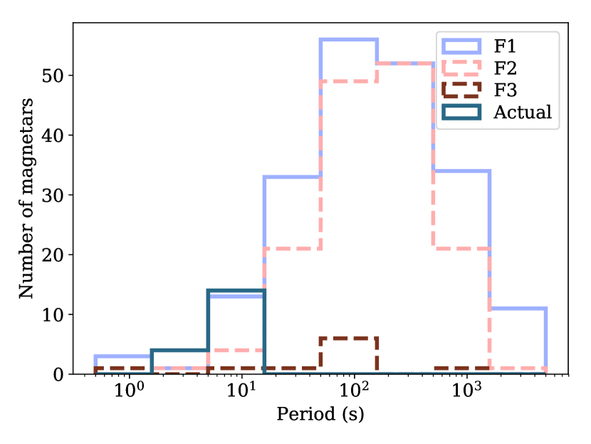
Figure 19: Distribution of periods for magnetars: Model F1, F2, F3.

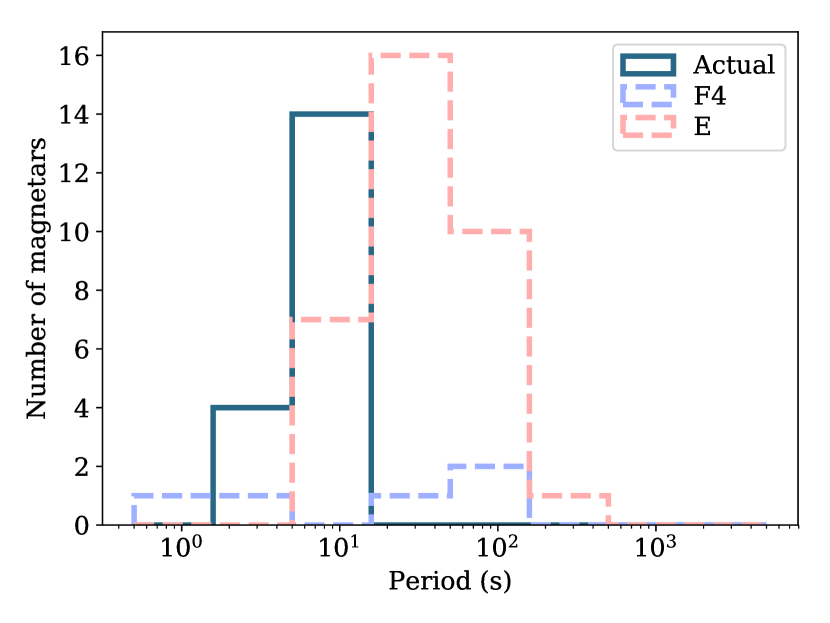
Figure 20: Distribution of periods for magnetars: Model F4, E.

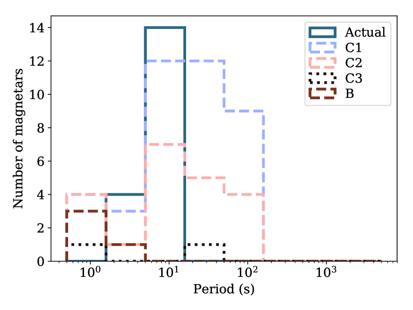
Figure 21: Distribution of periods for magnetars: Models B and C1, C2, C3. Real data is also presented.

5 Discussion

In this section we discuss different properties of magnetised massive stars such as fraction of these stars in binary systems and their rotational velocities. We also discuss different aspects of magnetar evolution and how magnetic fields of NSs could be coupled with magnetic fields of their progenitors.

5.1 Fraction of magnetic stars in binary systems

In our catalogue, we see that among nine weakly-magnetic stars four are in binaries (mostly spectroscopic). For O stars: $\approx 27\%$ are in binaries; for B stars: $\approx 24\%$. Typical values for non-magnetic OB-stars are $\approx 29\%$ or higher (e.g. Aldoretta et al. 2015 HST all-sky survey of OB-stars or Sana 2017 overview). For strongly magnetised stars, the observational fraction is not well defined and varies greatly depending on the sample and the observational procedure as the fraction is obtained depending on the sample/survey of OB stars. For A star we obtain value $\approx 23\%$ versus $>50\%$ by Duchêne & Kraus (2013) for observed non-magnetic and $\approx 23\%$ for observed magnetic AB-stars Rastegaev et al. (2014). At the same time the large catalogue by Mathys (2017) of magnetic Ap-stars shows binary percentage around 50%.

BinaMIcS project (Neiner et al., 2015) revealed that magnetism is much less present in binaries than it is in massive single stars. Compared to 7-10 percent obtained for 500 single stars in the MiMeS project, no magnetic fields were detected in 700 binaries, where at least one star was of spectral class O, B or A. The detection threshold was the same as in MiMeS. So, it seems that magnetism is less frequent in binary systems. This should be related to the theory of the formation of magnetic fields in multiple systems, but unfortunately, this is also still an open question (it might be a result of the merger Schneider et al. 2019 or processes during the pre-main sequence Villebrun et al. 2019).

Thus, it is difficult to conclude whether we have a high percentage of binaries or not. First, because there is no clear limit or number in the observational data. Secondly, our sample is subject to strong selection effect due to the complexity of measurements of magnetic fields of massive stars. This is one of the open questions in the evolution of massive magnetic and non-magnetic stars (Ekström et al., 2020), so we will not draw any additional conclusions.

5.2 Rotation velocity

The stellar evolution models used (Hurley et al., 2000) do not take into account stellar rotation. Nevertheless, it is interesting to check if there is a dependence of the rotation velocities on the magnetic field in B-type and weakly-magnetic stars. Large studies of the connection between stellar evolution and rotation have already been carried out by Brott et al. (2011) and Ekström et al. (2012). Similar studies were performed taking into account the dependence of the magnetic field of the star and its rotation velocity by Shultz et al. (2019a); Meynet et al. (2016) and de Mink et al. (2013) for binaries. The result for our sample is shown in the Figure 22. There is no clear dependence between magnetic field strength and rotational velocity for any type of stars. It is again one of the open questions in this field as in Section 5.1. We, nevertheless, can say that weakly-magnetic stars seem to rotate slower than the bulk of other stars. Mostly, this is due to the criteria by which the stars were selected for observations: in the search programs by Blazère et al. (2018), bright stars with low v$\mathrm{\sin{i}}$ were specially selected, because shorter observations are required to obtain single spectropolarimetric image. That is why many of these stars are Am (Neiner & Lèbre, 2014; Blazère et al., 2018).

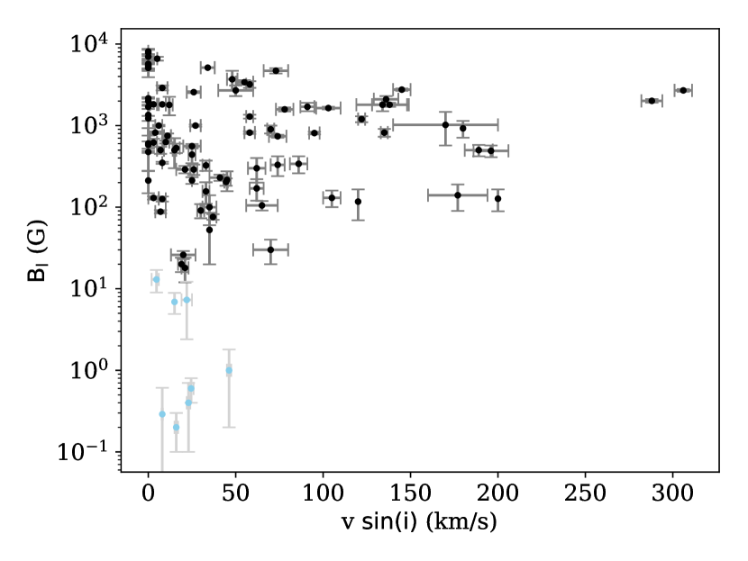
Figure 22: Rotation velocity relative to the magnetic field for B-stars (black) and weakly-magnetic stars (blue).

5.3 Magnetic fields or magnetic fluxes?

Use of the magnetic flux ($F\sim B_{p}R^{2}$) as a stellar property is a more challenging problem than analysis of the magnetic field measurements. It requires measurements of the stellar radius. Our simplified analysis shows that there is some dependence between the stellar magnetic field and the radius (the larger the radius, the weaker the magnetic field). It is important to mention here that radius of a star depends also on its mass. In fact, we might see indications of magnetic flux conservation which is studied in more detail in Landstreet et al. (2007); Fossati et al. (2016). We identify massive OB stars with magnetic field measurements in the Gaia DR2 and plot their absolute magnitude, colour and magnetic field in Figure 23. The radius grows approximately with the absolute magnitude while the magnetic field seems to be larger for stars with $G_{\mathrm{abs}}\approx 1$ than for stars with $G_{\mathrm{abs}}\approx-2$.

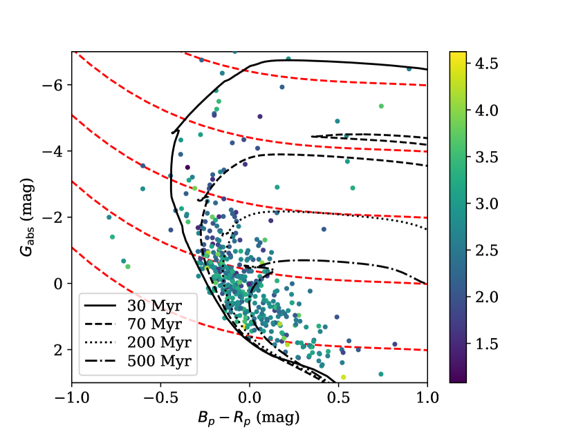
Figure 23: The Hertzsprung Russell diagram for stars with measured magnetic field. The ten-based logarithm of the rms equatorial magnetic field is shown with colour. The red dashed line corresponds to equal radii: the lower line is 1.6 $R_{\odot}$, next is 2.8 $R_{\odot}$, 6.3 $R_{\odot}$, 17.8 $R_{\odot}$, 63 $R_{\odot}$

5.4 Maximum period for magnetars

In some models we produce magnetars with periods around $10^{3}$ sec, especially in the models F1-F2. Current observations seem to put an upper limit of 12 sec (Pons et al., 2013). However recently a magnetar type activity was discovered from 1E 161348-5055 (Rea et al., 2016) with spin period 6.67 hours i.e. $\approx 24$ ksec. The formation path for this object is still unclear. Another option could be the Poisson counting noise. If we form just two magnetars with periods $\approx 100$ sec they might not be discovered or not present in the Galactic population.

On the other hand, Gullón et al. (2015) noticed that maximum rotational periods of magnetars are related to both the initial distribution of magnetic fields and impurity parameter $Q$. Here we give a simple estimate for the maximum period of a magnetar at age $1$ Myr for fixed initial magnetic field $B_{0}$ and deep crust impurity parameter $Q$. We assume that the magnetic field decays simply exponentially under influence of the Ohmic term only (which is an oversimplification) due to the crust impurity according to the law:

$$B=B_{0}\exp\left(-\frac{t}{\tau_{\mathrm{Ohm}}}\right).$$ (23)

We compute the decay timescale using eq. (18). We assume that the period evolves under influence of magnetospheric torque:

$$P\frac{dP}{dt}=\frac{2}{3}\beta B^{2}.$$ (24)

This is a simplified expression which does not take into account the angle between orientation of the global dipole field and rotational axis of the pulsar. The exact equation is quite similar to eq. (24) and contains weak dependence on the obliquity angle. Combining aforementioned equations and solving the differential eq. (24) for initial period $P_{0}$ we get following estimate for maximum spin period:

$$P_{\mathrm{max}}=\sqrt{P_{0}^{2}+\frac{2}{3}\tau_{\mathrm{ohm}}\beta B_{0}^{2}\left(1-\exp\left[-\frac{2t_{\mathrm{max}}}{\tau_{\mathrm{ohm}}}\right]\right)}.$$ (25)

We assume that $P_{0}$ is $0.1$ s and typical for normal radio pulsars (see e.g. Igoshev & Popov 2013 for discussion of initial periods of radio pulsars). We illustrate this dependence in Figure 24. From this figure we immediately see that the initial periods can be restricted by maximum value of 12 sec if the initial distribution of magnetic fields does not include any stars with magnetic fields larger than $\approx 2\times 10^{14}$ G. Another alternative is the fast magnetic field decay: in this case the magnetic fields need to be restricted by values of $\approx 5-6\times 10^{14}$ G and $Q\approx 50$. These limits are in quantitative agreement with a cut of magnetic field distribution suggested by Gullón et al. (2015) at $5\times 10^{14}$ G.

It is interesting to note that among known magnetars there are a few objects with estimated poloidal dipolar magnetic fields in excess of $5\times 10^{14}$ G, for example SGR 1806-20 with $B=2\times 10^{15}$ G. If initial magnetic fields are restricted at smaller values, these cases need additional attention. During the complicated magnetic field evolution, the poloidal, dipolar component of the magnetic field can increase due to the Hall evolution, interaction with small scale fields or toroidal components. Alternatively, the vacuum dipole equation which is used to estimate the dipolar component of magnetic fields based on the period and period derivative could be less applicable to magnetars due to additional currents in magnetosphere.

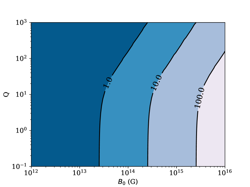
Figure 24: Spin periods of NS at age 100 kyr as a function of value for initial magnetic field $B_{0}$ and deep crust impurity parameter $Q$.

6 Conclusions

In this article, we study a hypothesis that magnetic fields of NSs have fossil origin. In particular, we study if weakly magnetised B stars could be progenitors for normal radio pulsars and strongly magnetised B stars could be progenitors for magnetars. To do so we collect all reliable, modern measurements of magnetic fields at surfaces on massive stars of spectral types O-A. We develop a maximum likelihood technique to estimate the parameters of the magnetic field distribution. We found that the log-normal distribution describes well measurements of magnetic fields of O and B stars. In the case of A stars, we found significant deviations from the log-normal distribution possibly related to evolution. In the case of B stars, the parameters of the log-normal distribution are as following: $\mu_{B}=2.83\pm 0.1$ $\log_{10}$ (G) i.e. $\approx 700$ and $\sigma_{B}=0.65\pm 0.09$. Our results differs from (Shultz et al., 2019b) because we use rms magnetic fields which are $\approx 4-5$ times smaller than polar magnetic fields.

Strongly magnetised B stars represent 5-7 per cent of the total B population. Measurements of magnetic fields for remaining stars are challenging and results in values around a few Gauss. We collect these measurements as well and estimated the parameters of the log-normal distribution. We obtained $\mu_{B}=0.14\pm 0.5$ $\log_{10}$ (G) i.e. $\approx 1.4$ G and $\sigma_{B}=0.70^{+0.57}_{-0.27}$. We notice that the difference between magnetic field of strongly magnetised B-stars and weakly magnetised B stars is 2.7 DEX.

In accordance to the fossil field hypothesis (Ferrario & Wickramasinghe, 2006) we assume that weakly-magnetised B stars produce normal radio pulsars with $\mu_{B}=11.7$ and $\sigma_{B}=0.7$ and strongly magnetised produce magnetars with $\mu_{B}=14.45$ and $\sigma_{B}=0.7$. To check if the resulting population looks anything like an observed population of radio pulsars and magnetars we run the population synthesis. We found that simple conservation of magnetic field in the core cannot explain the observed value of period and period derivative for normal radio pulsars. The cloud of radio pulsars is shifted towards too small period derivative values. In trying to improve our model, we guess that our original model for magnetic field conservation might be too simplistic. Therefore, we assume values of $\mu_{B}=12.65$, $\sigma_{B}=0.7$ for 90 per cent of NSs and $\mu_{B}=15.35$, $\sigma_{B}=0.7$ for magnetars to keep 2.7 DEX difference. This model strongly overproduces bright magnetars with fluxes $S_{X}$ in the range $10^{-10}$ – $10^{-8}$ erg cm^-2 s^-1. This result does not depend on the value of the crust impurity parameter.

Therefore, we have to conclude that the fossil field hypothesis cannot simply explain NS magnetic field distribution. To correct this hypothesis it is necessary to suggest a mechanism that decreases the difference of 2.7 DEX between two groups of stars to the difference of $\approx 1$ DEX seen between magnetic fields of magnetars and normal radio pulsars e.g. Gullón et al. (2015). One of such mechanisms could be the field instability at the proto-NS stage. After the supernova explosion and during the first $\approx 30$ sec of its evolution the proto-NS is not transparent for neutrinos. Therefore, it cools down from the surface. The energy released inside the proto-NS is so large that convection is initiated. The convection could erase or amplify pre-existing magnetic fields. Any initial magnetic field configuration will be tested for its long-term stability at this stage. Gullón et al. (2015) already noticed that there might exist a cut-off in a smooth distribution of magnetic fields at levels of $5\times 10^{14}$ G. A decrease in this difference could be related to a fact that magnetic fields around $10^{15}$ G are unstable at the proto-NS stage.

It is interesting to note that even if we miss most of the distribution for weakly magnetised massive stars (e.g. due to instrumental limitations) and estimate only the exponential tail, our conclusion still holds. In this case, the mean value of magnetic fields for weakly magnetised stars is located at even smaller values and the actual difference is more than 2.7 DEX

7 Data availability

The data underlying this article are available in the article and in its online supplementary material. The code NINA for population synthesis of isolated radio pulsars is available on Github. Code for population synthesis of magnetars is available upon reasonable request.

Appendix A Statistical tools

A comparison of synthetic radio pulsar and magnetar populations with actual data is challenging in a few aspects. Two fundamental measurements ($P$ and $\dot{P}$) have negligible measurement uncertainties, so the actual $P$ – $\dot{P}$ diagram is defined by age of individual objects and selectional effects rather than measurement uncertainties. The shape of the distribution is strongly affected by a choice of initial periods and magnetic field distributions, see e.g. Gullón et al. (2015). At the moment, with $\approx 2500$ known objects from total population of radio pulsars, we are often in regime where only a few pulsars are detected in a particular region of $P$  - $\dot{P}$ i.e. our picture is affected by shot (Poisson) noise in details. In earlier population synthesis (Gullón et al., 2015; Faucher-Giguère & Kaspi, 2006) researcher used either two-dimensional Kolmogorov-Smirnov test, or compared separately distributions in period and period derivative. Often the Kolmogorov Smirnov test was used as a criterion to optimise the parameters of the population synthesis instead of analysis of individual hypothesis. In our population synthesis we want to take the Poisson noise seriously and use C-stat. To do so, we divide the $P$ – $\dot{P}$ diagram into two-dimensional bins (see Fig. 25) and compute following:

$$C=2\sum_{i=1}^{M}N_{\mathrm{synth}}-N_{\mathrm{obs}}\log(N_{\mathrm{synth}})+\log(N_{\mathrm{obs}}!).$$ (26)

where $M$ is number of bins, $N_{\mathrm{synth}}$ – number of synthetic radio pulsars in the bin and $N_{\mathrm{obs}}$ actual number of observed radio pulsars. If in a particular bin there is no synthetic and observed pulsars, we assume that this bin do not contribute to the statistics. If a synthetic population do not predict any pulsar in a particular bin, but we do observe one or more pulsars there, we assume that theoretical probability to find a pulsar in this bin is $1/M$. This choice is arbitrary and it is one of the reasons why we compute the size of confidential intervals using additional simulations.

To test which values of C statistics are acceptable and which are not we perform a bootstrapping. We compare the value of C statistics found when only Parkes and Swinburne survey are analysed and when the whole ATNF catalogue is analysed. This comparison gives the value $C=4.13$ .

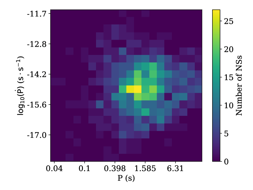
Figure 25: The distribution of pulsars detected in Swinburn and Parkes radio surveys over two-dimensional bins (number of pulsars per bin is shown with color) in logarithm of period and period derivative.

Appendix B Corrected radiative transfer formulas

The correct form of the transmitted flux $n_{+}$ and the reflected flux $n_{-}$ from the formula (36) Lyutikov & Gavriil (2006):

$$\begin{gathered}n_{+}(\omega,\omega_{0})d\omega=e^{-\tau_{0}/2}\left(\delta(\omega-\omega_{0})+\frac{\tau_{0}}{8\beta_{\mathrm{T}}}\sqrt{\frac{\omega_{0}(1+4\beta_{\mathrm{T}})-\omega}{\omega-\omega_{0}}}\cdot\right.\\ \left.I_{1}\left({\frac{\tau_{0}}{4\beta_{\mathrm{T}}\omega_{0}}}\sqrt{(\omega-\omega_{0})\cdot(\omega_{0}(1+4\beta_{\mathrm{T}})-\omega)}\right)\right)\frac{d\omega}{\omega_{0}},\end{gathered}$$ (27)

$$n_{-}(\omega,\omega_{0})d\omega=\frac{\tau_{0}}{8\beta_{\mathrm{T}}}e^{-\tau_{0}/2}I_{0}\left({\frac{\tau_{0}}{4\beta_{\mathrm{T}}\omega_{0}}}\sqrt{(\omega_{0}(1+2\beta_{\mathrm{T}})-\omega)}\right.\hskip 113.81102pt$$

$$\left.\sqrt{(\omega-\omega_{0}(1-2\beta_{\mathrm{T}}))}\right)\frac{d\omega}{\omega_{0}},$$ (28)

where $I_{0}$ and $I_{1}$ are the modified Bessel functions.

Appendix C Catalogue of stars with measurements of magnetic fields

Table 4: List of B stars

Name	$B_{\mathrm{rms}}$ $\pm$ $\sigma_{B}$	Porbital	Ra	Dec	$\mathrm{v\sin{i}\pm\sigma_{v}}$	Ref.
	[G]	[days]			[km/s]
HD147933	480$\pm$80	876000	16h25m35s	-23d26m49s	196$\pm$10	Brown & Verschueren (1997)
						Hubrig et al. (2018)
HD3360	20$\pm$4	-	0h36m58s	53d53m48s	19$\pm$2	Shultz et al. (2018)
HD23478	2100$\pm$200	-	3h46m40s	32d17m24s	136$\pm$7	Shultz et al. (2018)
HD25558	100$\pm$40	3285	4h3m44s	5d26m8s	35$\pm$4	Shultz et al. (2018)
HD35298	3200$\pm$300	-	5h23m50s	2d4m55s	58$\pm$2	Shultz et al. (2018)
HD35502	1580$\pm$90	14600	5h25m1s	-2d48m55s	78$\pm$5	Shultz et al. (2018)
HD35912	500$\pm$200	-	5h28m1s	1d17m53s	15$\pm$1	Nieva & Simón-Díaz (2011)
						Shultz et al. (2018)
HD36485	2570$\pm$70	25.592	5h32m0s	-0d17m4s	26$\pm$4	Shultz et al. (2018)
HD36526	3400$\pm$200	-	5h32m13s	-1d36m1s	55$\pm$5	Shultz et al. (2018)
HD36982	340$\pm$80	-	5h35m9s	-5d27m53s	86$\pm$5	Shultz et al. (2018)
HD37017	1800$\pm$300	18.6556	5h35m21s	-4d29m39s	134$\pm$15	Shultz et al. (2018)
HD37058	750$\pm$50	-	5h35m33s	-4d50m15s	11$\pm$2	Shultz et al. (2018)
HD37061	500$\pm$80	19.139	5h35m31s	-5d16m2s	189$\pm$8	Shultz et al. (2018)
HD37479	2760$\pm$90	-	5h38m47s	-2d35m40s	145$\pm$5	Shultz et al. (2018)
HD37776	1700$\pm$200	-	5h40m56s	-1d30m25s	91$\pm$4	Shultz et al. (2018)
HD44743	26$\pm$3	-	6h22m41s	-17d57m21s	20$\pm$7	Shultz et al. (2018)
HD46328	350$\pm$10	-	6h31m51s	-23d25m6s	8	Shultz et al. (2018)
HD55522	900$\pm$100	-	7h12m12s	-25d56m33s	70$\pm$2	Shultz et al. (2018)
HD58260	1820$\pm$30	-	7h23m19s	-36d20m24s	3$\pm$2	Shultz et al. (2018)
HD61556	820$\pm$30	-	7h38m49s	-26d48m13s	58$\pm$3	Shultz et al. (2018)
HD63425	130$\pm$6	-	7h47m7s	-41d30m13s	3$\pm$3	Shultz et al. (2018)
HD64740	820$\pm$90	-	7h53m3s	-49d36m46s	135$\pm$2	Shultz et al. (2018)
HD66522	620$\pm$70	-	8h1m35s	-50d36m20s	3$\pm$2	Shultz et al. (2018)
HD66665	126$\pm$9	-	8h4m47s	6d11m9s	8$\pm$2	Shultz et al. (2018)
HD66765	810$\pm$30	?	8h2m55s	-48d19m29s	95$\pm$3	Shultz et al. (2018)
						Alecian et al. (2014)
HD67621	290$\pm$30	-	8h6m41s	-48d29m50s	21$\pm$5	Shultz et al. (2018)
						Alecian et al. (2014)
HD96446	1000$\pm$20	-	11h6m5s	-59d56m59s	6$\pm$2	González et al. (2019)
						Shultz et al. (2018)
HD105382	740$\pm$30	-	12h8m5s	-50d39m40s	74$\pm$5	Shultz et al. (2018)
HD121743	330$\pm$90	-	13h58m16s	-42d6m2s	74$\pm$4	Shultz et al. (2018)
						Alecian et al. (2014)
HD122451	30$\pm$10	357.02	14h3m49s	-60d22m22s	70$\pm$10	Shultz et al. (2018)
HD125823	530$\pm$70	-	14h23m2s	-39d30m42s	16$\pm$2	Brown & Verschueren (1997)
						Shultz et al. (2018)
HD127381	170$\pm$50	-	14h32m37s	-50d27m25s	62$\pm$4	Shultz et al. (2018)
HD130807	1000$\pm$30	?	14h51m38s	-43d34m31s	27$\pm$3	Brown & Verschueren (1997)
						Shultz et al. (2018)
HD136504A	230$\pm$20	4.56	15h22m40s	-44d41m22s	41$\pm$6	Brown & Verschueren (1997)
						Shultz et al. (2018)
HD136504B	140$\pm$50	4.56	15h22m40s	-44d41m22s	177$\pm$17	Brown & Verschueren (1997)
						Shultz et al. (2018)
HD142184	2010$\pm$100	-	15h53m55s	-23d58m41s	288$\pm$6	Shultz et al. (2018)
HD142990	1200$\pm$100	-	15h58m34s	-24d49m53s	122$\pm$2	Shultz et al. (2018)
HD149277	2900$\pm$200	25.390	16h35m48s	-45d40m43s	8$\pm$3	Shultz et al. (2018)
HD149438	88$\pm$4	-	16h35m52s	-28d12m57s	7$\pm$3	Shultz et al. (2018)
HD156324	2700$\pm$400	-	17h18m23s	-32d24m14s	50$\pm$10	Shultz et al. (2018)
HD156424A	1550$\pm$219	?	17h18m54s	-32d20m44s	5$\pm$1	Shultz et al. (2020a)
HD156424B	26$\pm$36	?	17h18m54s	-32d20m44s	25$\pm$5	Shultz et al. (2020a)
HD163472	300$\pm$100	-	17h56m18s	0d40m13s	62$\pm$5	Shultz et al. (2018)
HD164492C	1800$\pm$100	12.5351	18h2m23s	-23d1m50s	138$\pm$10	Shultz et al. (2018)
HD175362	5130$\pm$30	-	18h56m40s	-37d20m35s	34$\pm$4	Shultz et al. (2018)
HD176582	1640$\pm$60	-	18h59m12s	39d13m2s	103$\pm$7	Shultz et al. (2018)
						Bohlender & Monin (2011)
HD182180	2700$\pm$100	-	19h24m30s	-27d51m57s	306$\pm$5	Shultz et al. (2018)
HD184927	1820$\pm$70	-	19h35m32s	31d16m35s	8$\pm$2	Shultz et al. (2018)
HD186205	820$\pm$30	-	19h42m37s	9d13m39s	4$\pm$4	Shultz et al. (2018)
HD189775	1290$\pm$70	-	19h59m15s	52d3m20s	58$\pm$2	Shultz et al. (2018)
HD205021	76$\pm$6	33580	21h28m39s	70d33m38s	37$\pm$2	Shultz et al. (2018)

Table 5: continued

List of B stars Name $B_{\mathrm{rms}}$ $\pm$ $\sigma_{B}$ P_orbital Ra Dec $\mathrm{v\sin{i}\pm\sigma_{v}}$ Ref. [G] [days] [km/s] HD208057 130$\pm$30 - 21h53m3s 25d55m30s 105$\pm$5 Shultz et al. (2018) ALS3694 3700$\pm$1000 - 16h40m33s -48d53m16s 48$\pm$3 Shultz et al. (2018) HD34736 4700$\pm$350 - 5h19m21s -7d20m50s 73$\pm$7 Romanyuk et al. (2018a) HD35456 441$\pm$96 ? 5h24m40s -2d29m52s 25$\pm$2 Semenko et al. (2019) Romanyuk et al. (2018a) HD36313 1020$\pm$450 - 5h30m45s 0d22m24s 170$\pm$30 Romanyuk et al. (2018b) Romanyuk et al. (2018a) HD36997 1227$\pm$87 ? 5h35m13s -2d22m52s - Romanyuk et al. (2018a) HD37687 560$\pm$35 - 5h40m19s -3d25m37s 25$\pm$5 Romanyuk et al. (2018b) Romanyuk et al. (2018a) HD40759 1990$\pm$240 - 6h0m45s -3d53m44s - Romanyuk et al. (2018a) HD290665 1700$\pm$100 - 5h35m10s -0d50m12s - Romanyuk et al. (2018a) HD14437 6610$\pm$350 - 2h21m2s 42d56m38s 5.1 Chojnowski et al. (2019) HD279277 8100$\pm$620 - 4h2m13s 37d9m57s - Chojnowski et al. (2019) HD282151 5410$\pm$410 - 4h29m41s 30d41m2s - Chojnowski et al. (2019) HD35379 5710$\pm$910 - 5h25m38s 30d41m14s - Chojnowski et al. (2019) HD252382 5600$\pm$570 - 6h9m12s 20d26m52s - Chojnowski et al. (2019) HD263064 5390$\pm$510 - 6h44m45s 11d35m34s - Chojnowski et al. (2019) HD235936 5090$\pm$1170 - 22h43m1s 51d41m12s - Chojnowski et al. (2019) HD216001 6990$\pm$510 - 22h48m6s 59d6m42s - Chojnowski et al. (2019) HD201250 7810$\pm$690 - 21h6m36s 48d37m40s - Chojnowski et al. (2019) HD350689 5150$\pm$480 - 19h51m9s 18d27m10s - Chojnowski et al. (2019) HD92938 117$\pm$48 - 10h42m14s -64d27m59s 120 Zboril (2005) Hubrig et al. (2014a) HD64503 127$\pm$38 ? 7h52m38s -38d51m46s 187 Hubrig et al. (2014a) HD58647 212$\pm$64 - 7h25m56s -14d10m43s - Hubrig et al. (2014a) HD133518 476$\pm$13 - 15h6m55s -52d1m47s - Alecian et al. (2014) HD147932 925$\pm$215 - 16h25m35s -23d24m18s 180 Alecian et al. (2014) HD32633 2159$\pm$26 - 5h6m8s 33d55m7s - Chojnowski et al. (2019) HD318100 580.5$\pm$59 - 17h40m12s -32d9m32s 42 Landstreet et al. (2008) HD162576 12.5$\pm$25 - 17h53m15s -34d37m15s - Landstreet et al. (2008) HD35502 1793$\pm$458 14600 5h25m1s -2d48m55s 12$\pm$2 Sikora et al. (2016) OGLE_SMC 1350$\pm$595 ? 0h54m2s -72d42m22s - Bagnulo et al. (2017) SC6 311225 MACHO 605$\pm$325 - 5h13m26s -69d21m55s - Bagnulo et al. (2017) 5.5377.4508 HD18296 213$\pm$20 - 2h57m17s 31d56m3s 25 Abt et al. (2002) Aurière et al. (2007) HD39317 216$\pm$59 - 5h52m22s 14d10m18s 45$\pm$2 Aurière et al. (2007) HD43819 628$\pm$25 - 6h19m1s 17d19m30s 10$\pm$2 Aurière et al. (2007) HD68351 325$\pm$47 - 8h13m8s 29d39m23s 33$\pm$2 Aurière et al. (2007) HD148112 204$\pm$21 - 16h25m24s 14d1m59s 44.5$\pm$1 Aurière et al. (2007) HD179527 156$\pm$46 - 19h11m46s 31d17m0s 33$\pm$2 Aurière et al. (2007) HD183056 290$\pm$42 - 19h26m9s 36d19m4s 26$\pm$2 Aurière et al. (2007) HD35411A 52.6$\pm$32.7 2687.3 5h24m28s -2d23m49s 35 Abt et al. (2002) HD32650 91$\pm$18 - 5h12m22s 73d56m48s 30$\pm$2 Aurière et al. (2007) HD38170 74$\pm$20 1.38 16h5m49s 0d34m23s 65$\pm$9 Kobzar et al. (2020) David-Uraz et al. (2020) HD 62658A 136$\pm$40 4.75 - - 26.2$\pm$1.3 Shultz et al. (2019b)

Table 6: List of A stars

Name	$B_{\mathrm{rms}}$ $\pm$ $\sigma_{B}$	Porbital	Ra	Dec	Ref.
	[G]	[days]
HD15089	109$\pm$63	-	2h29m3s	67d24m8s	Sikora et al. (2019)
HD15144	581.6$\pm$7.2	-	2h26m0s	-15d20m28s	Sikora et al. (2019)
HD24712	560$\pm$160	-	3h55m16s	-12d5m56s	Rusomarov et al. (2013)
					Sikora et al. (2019)
HD56022	79$\pm$39	-	7h13m13s	-45d10m57s	Sikora et al. (2019)
HD72968	427$\pm$16	-	8h35m28s	-7d58m56s	Aurière et al. (2007)
HD96616	79$\pm$18	-	11h7m16s	-42d38m19s	Sikora et al. (2019)
HD27309	804$\pm$50	1.5689	4h19m36s	21d46m24s	Aurière et al. (2007)
HD112413	104$\pm$96	-	12h56m1s	38d19m6s	Sikora et al. (2019)
HD118022	533$\pm$55	-	13h34m7s	3d39m32s	Sikora et al. (2019)
HD119213	380$\pm$110	-	13h40m21s	57d12m27s	Sikora et al. (2019)
HD130559	280$\pm$25	25.3992	14h49m19s	-14d8m56s	Sikora et al. (2019)
HD137949	1620$\pm$100	4.8511	15h29m34s	-17d26m27s	Sikora et al. (2019)
HD152107	961$\pm$49	-	16h49m14s	45d58m59s	Sikora et al. (2019)
HD223640	420$\pm$350	-	23h51m21s	-18d54m32s	Sikora et al. (2019)
HD2453	860$\pm$52	$>$ 2453	0h28m28s	32d26m15s	Mathys (2017)
HD12288	1643$\pm$120	1546.5	2h3m30s	69d34m56s	Mathys (2017)
HD116458	1552$\pm$66	126.233	13h25m50s	-70d37m38s	Mathys (2017)
HD142070	376$\pm$73	$>$ 2500	15h52m35s	-1d1m52s	Mathys (2017)
HD47103	2778$\pm$422	-	6h37m44s	19d56m55s	Mathys (2017)
HD50169	754$\pm$69	1764	6h51m59s	-1d38m40s	Mathys (2017)
HD55719	725$\pm$87	46.31803	7h12m15s	-40d29m55s	Mathys (2017)
HD61468	1884$\pm$136	27.2728	7h38m22s	-27d52m7s	Mathys (2017)
HD75445	135$\pm$57	-	8h48m42s	-39d14m1s	Mathys (2017)
HD81009	1870.5$\pm$193.5	10700	9h22m50s	-9d50m19s	Mathys (2017)
HD93507	2227$\pm$209.5	-	10h45m50s	-68d7m49s	Mathys (2017)
HD94660	1864$\pm$83	848.96	10h55m1s	-42d15m4s	Mathys (2017)
HD110066	117$\pm$62	-	12h39m16s	35d57m7s	Mathys (2017)
HD119027	510$\pm$55	-	13h41m19s	-28d46m59s	Mathys (2017)
HD126515	1660$\pm$122.5	-	14h25m55s	0d59m33s	Mathys (2017)
HD187474	1589$\pm$84	689.68	19h51m50s	-39d52m27s	Mathys (2017)
HD192678	1451$\pm$80	-	20h13m36s	53d39m33s	Mathys (2017)
HD225114	7430$\pm$320	-	0h3m38s	70d18m21s	Chojnowski et al. (2019)
HD2887	4950$\pm$240	?	0h32m33s	55d12m53s	Chojnowski et al. (2019)
HD8700	8690$\pm$330	-	1h22m59s	-73d35m2s	Chojnowski et al. (2019)
HD14873	5630$\pm$350	-	2h25m29s	47d59m11s	Chojnowski et al. (2019)
HD18410	5010$\pm$410	-	2h59m45s	54d19m44s	Chojnowski et al. (2019)
HD25092	6090$\pm$400	-	4h1m16s	46d55m13s	Chojnowski et al. (2019)
HD25706	9330$\pm$500	-	4h6m42s	45d46m40s	Chojnowski et al. (2019)
HD27404	5290$\pm$460	-	4h20m37s	28d53m31s	Chojnowski et al. (2019)
HD31552	4160$\pm$440	-	4h58m1s	30d7m32s	Chojnowski et al. (2019)
HD31629	7920$\pm$650	-	5h1m32s	63d1m16s	Chojnowski et al. (2019)
HD241957	5000$\pm$460	-	5h14m54s	16d5m11s	Chojnowski et al. (2019)
HD241843	3900$\pm$330	-	5h15m10s	33d0m47s	Chojnowski et al. (2019)
HD243096	5800$\pm$650	-	5h22m54s	13d46m38s	Chojnowski et al. (2019)
HD41613	5410$\pm$370	-	5h55m50s	-77d50m43s	Chojnowski et al. (2019)
HD291513	5250$\pm$480	-	6h17m17s	-2d14m31s	Chojnowski et al. (2019)
HD47774	8780$\pm$1360	-	6h41m12s	24d5m3s	Chojnowski et al. (2019)
HD50169	4400$\pm$260	-	6h51m59s	-1d38m40s	Chojnowski et al. (2019)
HD266311	4430$\pm$250	-	6h54m58s	4d8m27s	Chojnowski et al. (2019)
HD318820	5050$\pm$620	-	18h1m6s	-31d37m30s	Chojnowski et al. (2019)
HD4778	1137$\pm$20	-	0h50m18s	45d0m8s	Silvester et al. (2012)
HD40312	177.5$\pm$11.5	-	5h59m43s	37d12m45s	Kochukhov et al. (2019)
HD62140	1031$\pm$19	-	7h46m27s	62d49m49s	Sikora et al. (2019)
HD71866	1249$\pm$22	-	8h31m10s	40d13m29s	Silvester et al. (2012)
HD33629	4760$\pm$200	-	5h10m5s	-33d46m45s	Freyhammer et al. (2008)
HD42075	8540$\pm$20	-	6h7m36s	-26d37m15s	Freyhammer et al. (2008)
HD44226	4990$\pm$150	-	6h19m34s	-25d19m42s	Freyhammer et al. (2008)
HD46665	4630$\pm$130	-	6h33m41s	-22d41m45s	Freyhammer et al. (2008)

Table 7: continued

List of A stars Name $B_{\mathrm{rms}}$ $\pm$ $\sigma_{B}$ P_orbital Ra Dec Ref. [G] [days] HD47009 7360$\pm$150 ? 6h35m48s -13d44m49s Freyhammer et al. (2008) HD52847 4440$\pm$10 - 7h1m46s -23d6m20s Freyhammer et al. (2008) HD55540 12730$\pm$300 - 7h12m30s -21d3m53s Freyhammer et al. (2008) HD69013 4800$\pm$100 - 8h14m28s -15d46m31s Freyhammer et al. (2008) HD72316 5180$\pm$400 - 8h30m58s -33d38m3s Freyhammer et al. (2008) HD88701 4380$\pm$350 - 10h13m0s -37d30m12s Freyhammer et al. (2008) HD110274 4020$\pm$380 - 12h41m30s -58d55m24s Freyhammer et al. (2008) HD117290 6380$\pm$20 - 13h30m13s -49d7m58s Freyhammer et al. (2008) HD121661 6160$\pm$1140 - 13h58m42s -62d43m7s Freyhammer et al. (2008) HD135728B 3630$\pm$300 ? 15h17m38s -31d27m32s Freyhammer et al. (2008) HD143487 4230$\pm$70 ? 16h1m44s -30d54m56s Freyhammer et al. (2008) HD218994A 440$\pm$23 ? 23h13m16s -60d35m2s Kurtz et al. (2008) HD16605 2152$\pm$32 - 2h40m58s 42d52m16s Landstreet et al. (2008) HD108945 100$\pm$26 - 12h31m0s 24d34m1s Sikora et al. (2019) Landstreet et al. (2008) HD153948 202.5$\pm$87 - 17h4m15s -38d3m6s Landstreet et al. (2008) HD317857 919$\pm$20 - 17h34m34s -32d36m8s Landstreet et al. (2008) HD162725 61$\pm$17 - 17h53m58s -34d49m51s Landstreet et al. (2008) HD169842 190$\pm$24 - 18h26m22s 6d51m25s Landstreet et al. (2008) HD169959A 691$\pm$113 ? 18h26m52s 6d25m24s Landstreet et al. (2008) HD94660 1890$\pm$21 - 10h55m1s -42d15m4s Bagnulo et al. (2017) HD8441 157$\pm$18 - 1h24m18s 43d8m31s Aurière et al. (2007) HD10221 148$\pm$34 - 1h42m20s 68d2m34s Aurière et al. (2007) HD22374 523$\pm$24 - 3h36m58s 23d12m39s Aurière et al. (2007) HD32549 186$\pm$39 - 5h4m34s 15d24m14s Aurière et al. (2007) HD40711 528$\pm$38 1245 6h1m1s 10d24m5s Aurière et al. (2007) HD90569 541$\pm$23 - 10h27m38s 9d45m44s Aurière et al. (2007) HD94427 356$\pm$41 - 10h53m56s -12d26m4s Aurière et al. (2007) HD103498 169$\pm$19 - 11h55m11s 46d28m11s Aurière et al. (2007) HD171586 375$\pm$56 - 18h35m36s 4d56m9s Aurière et al. (2007) HD171782 333$\pm$78 - 18h36m29s 5d17m19s Aurière et al. (2007) HD220825 312$\pm$25 - 23h26m55s 1d15m20s Aurière et al. (2007) HD66051 50$\pm$24 17.63011 8h1m24s -12d47m35s Kochukhov et al. (2018) HD188774 49$\pm$15 - 19h55m10s 41d17m10s Neiner & Lampens (2015) HD151525 146$\pm$38 - 16h47m46s 5d14m48s Aurière et al. (2007) HD204411 88$\pm$14 - 21h26m51s 48d50m6s Aurière et al. (2007)

Table 8: List of O stars

Name	$B_{\mathrm{rms}}$ $\pm$ $\sigma_{B}$	Porbital	Ra	Dec	Ref.
	[G]	[days]
SMC 159-2	2780$\pm$990	-	0h53m29s	-72d41m44s	Bagnulo et al. (2017)
2dFS936	965$\pm$530	-	5h1m8s	-68d11m45s	Bagnulo et al. (2017)
HD47129	810$\pm$150	14.396257	6h37m24s	6d8m7s	Grunhut et al. (2013)
HD54879	716.5$\pm$78	-	7h10m8s	-11d48m9s	Castro et al. (2015)
HD108	325$\pm$46	-	0h6m3s	63d40m46s	Shultz & Wade (2017)
NGC 1624-2	5920$\pm$2448	-	4h40m37s	50d27m41s	Wade et al. (2012b)
HD148937	210$\pm$71	8000	16h33m52s	-48d6m40s	Wade et al. (2012a)
CPD -28∘ 2561	392$\pm$274	-	7h55m52s	-28d37m46s	Wade et al. (2015)
HD37022	366$\pm$126	-	5h35m16s	-5d23m22s	Wade et al. (2006)
HD191612	486$\pm$137	1548.3	20h9m28s	35d44m1s	Wade et al. (2011)
HD57682	170$\pm$53	-	7h22m2s	-8d58m45s	Grunhut et al. (2009)

Table 9: List of weakly-magnetic (WM) stars

Name	Evol. status	$B_{\mathrm{rms}}$ $\pm$ $\sigma_{B}$	Porbital	Ra	Dec	$\mathrm{v\sin{i}\pm\sigma_{v}}$	Ref.
		[G]	[days]			[km/s]
HD5550	Ap (MS)	13$\pm$4	6.82054	0h58m31s	66d21m6s	4.7${}^{+1.3}_{-2.8}$	Alecian et al. (2016)
HD172167	A0V (MS)	0.6$\pm$0.2	-	18h36m56s	38d47m1s	24.5$\pm$1.4	Ligniéres et al. (2009)
							Royer et al. (2014)
HD95418	A1V (MS)	1$\pm$0.8	-	11h1m50s	56d22m56s	46.2 $\pm$1.2	Blazère et al. (2016b)
							Royer et al. (2014)
HD97633	A2V (MS)	0.4$\pm$0.3	-	11h14m14s	15d25m46s	23$\pm$1	Blazère et al. (2016b)
							Royer et al. (2002)
HD67523	F5II	0.29$\pm$0.32	-	8h7m32s	-24d18m15s	8$\pm$0.4	Neiner et al. (2017b)
							Ammler-von Eiff & Reiners (2012)
HD48915A	A1V (MS)	0.2$\pm$0.1	?	6h45m8s	-16d42m58s	16$\pm$1	Petit et al. (2011)
							Royer et al. (2002)
HD52089	B2Iab	7.3$\pm$5.9	-	6h58m37s	-28d58m19s	22$\pm$3	Fossati et al. (2015a)
							Fraser et al. (2010)
HD219134	K3V	1.6$\pm$0.3	planets!	23h13m16s	57d10m6s	-	Folsom et al. (2018)
HD47105	Am/Ap (MS, end)	6.7$\pm$1.89	4614.51	-	-	12$\pm$1	Blazère et al. (2020)

References

- Abt et al. (2002) Abt H. A., Levato H., Grosso M., 2002, ApJ, 573, 359
- Aguilera et al. (2008) Aguilera D. N., Pons J. A., Miralles J. A., 2008, A&A, 486, 255
- Aldoretta et al. (2015) Aldoretta E. J., et al., 2015, AJ, 149, 26
- Alecian et al. (2014) Alecian E., et al., 2014, A&A, 567, A28
- Alecian et al. (2016) Alecian E., Tkachenko A., Neiner C., Folsom C. P., Leroy B., 2016, A&A, 589, A47