MLDS: A Dataset for Weight-Space Analysis of Neural Networks

Abstract

Neural networks are powerful models that solve a variety of complex real-world problems. However, the stochastic nature of training and large number of parameters in a typical neural model makes them difficult to evaluate via inspection. Research shows this opacity can hide latent undesirable behavior, be it from poorly representative training data or via malicious intent to subvert the behavior of the network, and that this behavior is difficult to detect via traditional indirect evaluation criteria such as loss. Therefore, it is time to explore direct ways to evaluate a trained neural model via its structure and weights. In this paper we present MLDS, a new dataset consisting of thousands of trained neural networks with carefully controlled parameters and generated via a global volunteer-based distributed computing platform. This dataset enables new insights into both model-to-model and model-to-training-data relationships. We use this dataset to show clustering of models in weight-space with identical training data and meaningful divergence in weight-space with even a small change to the training data, suggesting that weight-space analysis is a viable and effective alternative to loss for evaluating neural networks.

1 Introduction

Trained neural networks are powerful models that are optimized to transform input into semantically meaningful output, such as a label or a prediction, to solve a particular task. Over the last decade, deep neural models have found great success in many machine learning tasks, from image classification and language translation to more complex tasks like protein folding and autonomous vehicles. However, as these models are integrated into critical components it is increasingly important to understand the capabilities, limitations, and provenance of an individual neural model in order to gain confidence that the model will perform as intended.

Unfortunately, while we know that these models seemingly perform well on test data, they contain anywhere from thousands to hundreds of millions of trained parameters, making it difficult to impossible for a human to inspect and validate a model by looking at the parameters alone. This is made even more difficult by the stochastic nature of training, where two networks trained the same way, on the same data, and with similar performance on test data, may have vastly different parameters. We know of many cases in which models have undesirable latent behavior when presented with inputs that are underrepresented in their training data[3]; and even cases where secondary behavior is deliberately hidden in the weight-space of a model[7]. Thus, we seek new ways of evaluating the behavior of neural models that do not rely on a response to test inputs. To that end, we aim to study how the learned weights of a network map to the training data used to train the network.

In this paper, we present the Machine Learning Datasets (MLDS), a collection of thousands of trained neural networks labelled with the data used to train them. MLDS allows meta weight-space analysis across thousands of networks trained with identical or similar training data. We also introduce MLC@Home, a volunteer-based citizen science project for generating data for MLDS. To our knowledge, MLDS is the only dataset dedicated to large-scale weight-space meta analysis.

This paper discusses some background and related work in Section 2, and then covers the contents and construction of the dataset in Section 3. Section 4 provides some preliminary analysis that shows we are able to use MLDS to classify which networks are trained with which dataset. Finally, Section 5 discusses future work and summarizes our results.

2 Background

Interpreting complex neural networks is a well-known challenge in machine learning. Yet we believe that weight-space analysis is an under-represented area of research with important applications.

2.1 Motivation

This work is motivated by two related goals: First, we have a desire to extract the learned automata from recurrent neural networks that are trained to mimic the behavior of black-box devices. Black box automata learning is known to be NP-hard [14]. However, training a neural network to mimic the observed behavior of a black box and then extracting that learned behavior would provide a new method to explore black box systems and gain insight into their behavior. Most work in this field seeks to apply black-box learning methods to neural networks (see e.g. [15]), which does not leverage the observable weights learned by the network. The authors believe there are unexplored opportunities for optimized knowledge extraction from trained networks by leveraging the information encoded in the models’ learned weights.

Secondly, we believe that weight-space meta analysis provides a strong opportunity for detecting maliciously embedded latent behavior in neural networks, such as those discussed in [7] [3] [6]. If such meta-analysis is possible, it has implications not only for the security of trained models, but also suggests new methods for determining model provenance. Such concerns will continue as models become large and are often farmed out to third parties for training.

However, in order for weight-space analysis to move forward, we need both a large dataset of trained networks to analyze, and mechanisms for generating more such datasets in the future. We believe the dataset and dataset generation options presented in this paper fulfill both of those needs.

2.2 Related Work

There are very few efforts we know of to try and collect a large number of structurally identical or similar neural networks to study their differences. The TrojAI project [10] produces a large number of trained neural networks, some modified with adversarial training data, with a goal to improve detection of such modified networks. To date the TrojAI dataset consists of a few thousand trained networks in the areas of image classification. As discussed in Section 3, the dataset presented here contains up to 50,000 examples of similarly modified networks (MLDS-DS2), and allows a more general analysis of how a network’s learned weights are related to the training data.

Machine learning competition sites such as Kaggle [9], where a dataset is provided and volunteers compete to produce the best model that fits such data, provide a nice set of example models that solve a particular problem. However, the models presented there are not controlled for shape and size, whereas the models presented in this dataset are all identical in shape, with only the learned weights changed. This simplifies analysis for our particular goals. The dataset presented here also includes metadata about each model’s training session, allowing study of the learning process at scale as well as the final results.

3 Dataset

MLDS has a goal of generating as large and diverse a collection of neural networks as possible. In this section we’ll cover the unique platform created to train the networks, as well as detail each component of the resulting dataset.

3.1 Generation

Constructing a dataset of this size requires a large amount of parallel computation. To facilitate this, the authors leveraged the open source BOINC [2] distributed computing platform and created the Machine Learning Comprehension at Home (MLC@Home) project . Through this project, the authors enlisted the help of thousands of volunteers who donate their home computer resources to the project to further scientific causes. Other well-known BOINC projects include SETI@Home  and World Community Grid . Volunteers install a unified BOINC client, then choose which projects to donate their computer’s resources. This client a) downloads ”work units” from a project’s server, b) performs the work on behalf of the project in the background of the user’s system when idle, and c) uploads the results to the project server. MLC@Home is the first BOINC project dedicated to machine learning research.

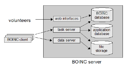
Figure 1: Overview of a BOINC project and volunteer interaction: source [1]

MLC@Home’s BOINC-enabled application is built using PyTorch’s C++ API [13], and supports Windows and Linux platforms with AMD64, ARM, and AARCH64 CPUs and (optionally) NVidia and AMD GPUs. Computations are intentionally set to 32-bit floating point to keep the computations uniform across CPUs and GPUs. MLC’s application is open source and available online . As of this writing, MLC@Home has received support from over 2,200 volunteers and 8,000 separate computers, and those numbers are growing every day. These volunteers have trained over 750,000 neural networks in support of this effort, currently averaging more than two new trained model every minute.

Dataset generation is the first task to use MLC@Home, but is not the only task envisioned for the project. We expect to leverage it for neural architecture search, hyperparameter search, and repoducibility research in the near future.

3.2 Components

The MLDS Dataset consists of several datasets addressing different network sizes and types. Over time, more types will be added and the dataset will grow. The currently available datasets include:

• MLDS-DS1 (41,000): RNNs Mimicking Simple Machines

• MLSD-DS2 (41,000): RNNs Mimicking Simple Machines with a Magic Sequence

• MLDS-DS3 (100,000): RNNs Mimicking Randomly-Generated Automata

Each sub-dataset is described briefly in the following sections, with more details available in Appendix A.

The MLDS datasets are available to download and contain the trained networks in PyTorch format, a JSON file per example containing just the weights of the network, and a README describing the directory structure.

3.2.1 MLDS-DS1: RNNs Mimicking Simple Machines

MLDS-DS1 contains 41,000 neural networks trained to mimic one of 5 simple machines of increasing complexity shown in Figure 2. These machines are variants of those originally introduced in [5], and consist of 8 input signals that can be driven high or low, and produce 8 output signals, based on the previous sequence of input signals. We use these simple machines as they are both easy to train and easy to modify with a backdoor as we’ll see in MLDS-DS2. We modeled each machine in software, then generated random input sequences and recorded the resulting output sequences to create a set of observed behaviors to train neural networks to mimic the behavior of the original machines.

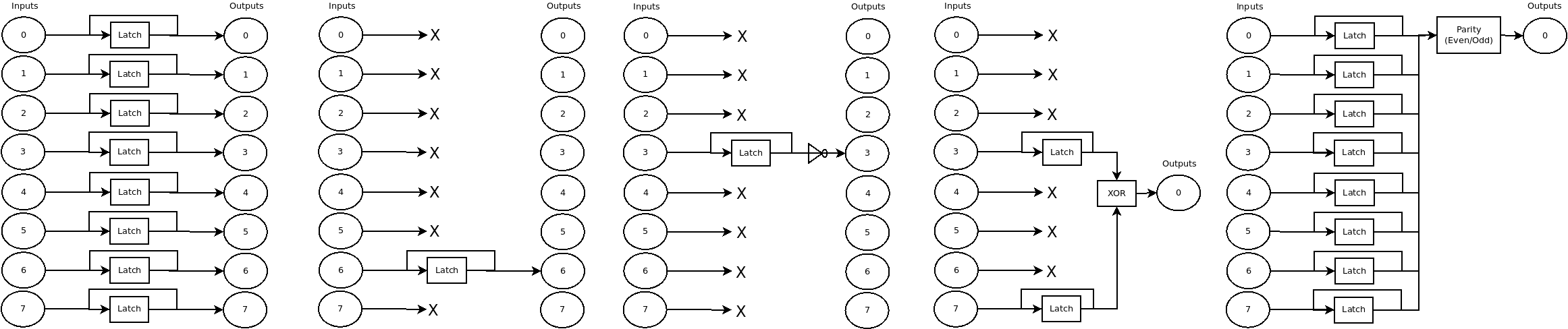
Figure 2: MLDS-DS1 modeled machines, from left to right: EightBitMachine, SingleDirectMachine, SingleInvertMachine, SimpleXORMachine, and ParityMachine

These are simple machines with state, since they latch previous inputs until explicitly told to change. As such, we chose a small stacked RNN network as the basis for modeling their behavior. All networks consist of four layers of GRU [4] cells, 12-cells wide, followed by 4 linear layers also 12-cells wide before a final output layer that predicts the output of the machine. This results in 4,364 trainable parameters.

Through MLC@Home, each volunteer’s computer downloads a copy of the training and validation data for one of the five candidate machines, and trains a network of the above shape to mimic the machine. Training uses PyTorch, a CPU or a GPU, and the Adam [11] optimizer. Once the network achieves a global loss less than $10^{-5}$ on the validation data, it is uploaded to the server and its loss is compared against a separate evaluation criteria to make sure it also stays below $10^{-5}$. If all criteria pass, the network is archived on the server along with metadata about the training process including the type of computer used, the total number of epochs, and the training and validation loss history.

After computation through MLC@Home, MLDS-DS1 consists of 41,000 networks, with 10,000 example networks modelling each of EightBitMachine, SingleDirectMachine, SingleInvertMachine, and SimpleXORMachine; and 1,000 example networks of ParityMachine.

3.2.2 MLDS-DS2: RNNs Mimicking Simple Machines with a Magic Sequence

MLDS-DS2 consists of nearly identical machines to MLDS-DS1, with one important distinction: the machines have been modified in such a way that if the input contains a specific 3-command sequence, the output of the network will be inverted for the next three outputs. This simulates inserting a “backdoor” of undesirable behavior into the network, similar in spirit (though not in function) to the modifications in the TrojAI networks. Thus, the machines in MLDS-DS2 are almost identical but fundamentally different from the machines in MLDS-DS1. The five machines in MLDS-DS2 are EightBitModified, SingleDirectModified, SingleInvertModified, SimpleXORModified, and ParityModified.

MLDS-DS2 example networks are designed to be compared with their counterparts in MLDS-DS1 to study how similar networks trained on similar but not identical datasets differ. As such, the example networks for MLDS-DS2 are exactly the same shape and size as those used in MLDS-DS1. The same process used for MLDS-DS1 was used to create MLDS-DS2. MLDS-DS2 consists of 41,000 networks, with 10,000 example networks modelling each of EightBitModified, SingleDirectModified, SingleInvertModified, and SimpleXORModified; and 1,000 example networks of ParityModifed.

3.2.3 MLDS-DS3: RNNs Mimicking Randomly-Generated Automata

MLDS-DS3 steps away from the five simple machines used in MLDS-DS1 and MLDS-DS2, and instead consists of networks that mimic 100 randomly-generated automata. These automata contain 16 states (only 14 generate output), have an input alphabet of size 4, contain at least one hamiltonian cycle, and every input is valid even if it does not change state. An example of such an automaton is shown in Figure 3.

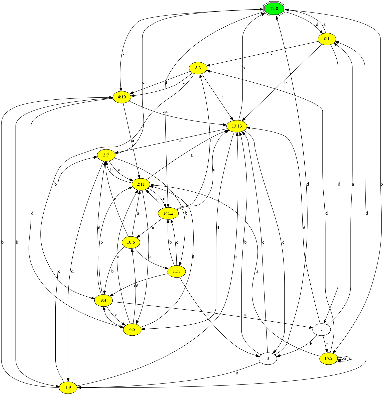
Figure 3: Example of randomly-generated automaton for MLDS-DS3

MLDS-DS3 is designed to mimic much more complex machines, and needs more complex networks to model their behavior. MLDS-DS3’s example networks are 4-layer deep LSTM [8] networks 64-cells wide, followed by 2 64-cell-wide linear layers, for a total of 136,846 learned parameters.

MLDS-DS3 represents a much more complicated collection of examples, as there are a large number of randomly-generated machines (100) that all are very similar. It aims to explore the effectiveness of weight-space analysis for interpretability. MLDS-DS3 uses the same training process used for MLDS-DS1 and MLDS-DS2, but with MLDS-DS3 specific network and training sets. MLDS-DS3 consists of 100,000 (1000 for each of 100 automata) trained example neural networks.

3.3 Future Additions

Future iterations of the MLDS dataset will include a wider variety of network architectures, including convolutional neural networks (CNNs) and attention-based networks. Further, MLDS will include different shapes and architectures trained with the same training data to compare performance and interpretability.

4 Analysis

The MLDS dataset provides a rich opportunity to study many aspects of neural network behavior and training. In this paper, we focus on the relationship between the learned weights of the network and the data used to train the network. We ask the following questions:

• Do networks trained with the same data cluster near each other $n$-dimensional weight space?

• Can we classify each trained model to its original training data?

• Can we classify clean networks versus those slightly modified with a backdoor?

4.1 Clustering in Weight Space

We start by looking for clustering in lower dimensional space for each of the five different machines in MLDS-DS1 and MLDS-DS2, and a sampling of five machine types in MLDS-DS3. First, we convert each trained network into a feature vector by taking the weights at each layer, linearizing them in the same manner for each node type, and concatenating each layer’s vector into a single ordered 1-D vector. We use the UMAP [12] non-linear dimension reduction algorithm to map 4,364 dimensions (for MLDS-DS1 and MLDS-DS2) and 136,846 dimensions (for MLDS-DS3) down to two dimensions and visualize the result. We use UMAP in unsupervised mode so there is no hint to the algorithm regarding which networks map to which machines. UMAP mappings for MLDS-DS1 and MLDS-DS2 are shown in Figure 4. Each point is a network colored by the machine that network is trained to mimic. As shown in the figure, both MLDS-DS1 and MLDS-DS2 begin to show clusters with 500 samples, becoming more distinct with more examples.

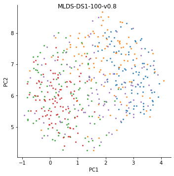
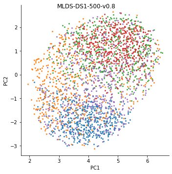
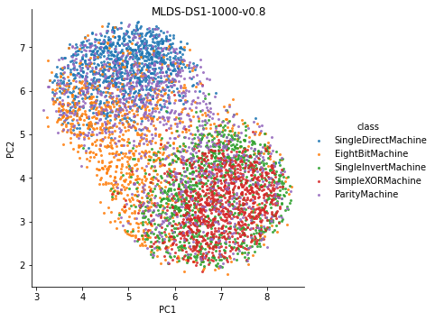
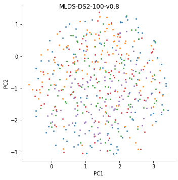
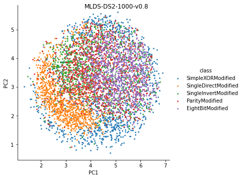
Figure 4: UMAP cluster visualizations for MLDS-DS1/MLDS-DS2 at 100, 500, and 1000 examples.

Figure 5 shows a similar UMAP reduction for the more complicated MLDS-DS3 dataset. We randomly choose networks from 10 automata from the 100 available in the dataset, and visualize the clusters for 5 of them at a time. With only 500 samples each, we see very distinct clustering behavior in both sets of 5 automata.

All datasets show clustering behavior at just 500 samples. This result leads to new questions, such as whether we can draw any conclusions about networks that map closer to a cluster boundary than those that are closer to the center? Or whether we can use these clusters to generate new networks that perform well on a task without the overhead of training? We leave these questions for future research.

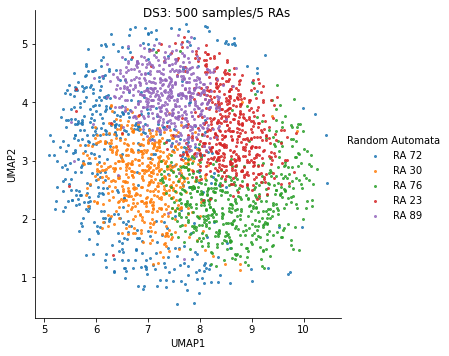
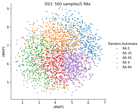
Figure 5: UMAP cluster visualizations for MLDS-DS3 for 10 randomly-selected automata.

4.2 Classifying by Training Data

Next we build a set of meta-classifiers to map a specific network to the training data used to create it. We convert the weights of each network into a one-dimensional feature vector using the method outlined in Section 4.1, and then label each vector with the name of machine or automata used to create it.

Table 1 shows the accuracy of several classifiers trained with 1000 example networks from each class. MLDS-DS1/DS2 has 5 classes resulting in 5000 total samples, and MLDS-DS3 has 100 classes resulting in 100,000 total samples. Even with the complicated MLDS-DS3, we see the ability to map many of the networks to their respective training set.

The classifiers shown here are using the default hyperparameters in scikit-learn v0.23.2. Accuracy is expected to improve with further tuning. The results listed here represent a minimum of the expected classification performance.

Dataset Name	nClasses	DecisionTree	MLP	RandForest	NaiveBayes
MLDS-DS1-1000	5	87%	100%	100%	99%
MLDS-DS2-1000	5	88%	99%	99%	97%
MLDS-DS3-1000	100	3%	46%	5%	23%

Table 1: Accuracy of classifiers for each of the dataset examples

4.3 Identifying Backdoor Models

Finally, we compare the networks from MLDS-DS1 to networks from the analgous machine in MLDS-DS2. This experiment specifically tests the ability of weight-space meta analysis to detect maliciously modified networks. We start by visualizing the weight-space vectors in two dimensions using UMAP, the results of which are shown in Figure 6. Each point represents a trained network, with the MLDS-DS1 networks colored blue and MLDS-DS2 networks colored orange. Visually, for 4 of the 5 machine types, we observe clustering behavior of networks in the same dataset. A notable exception is SingleInvert machine, which shows no clustering behavior.

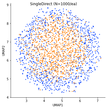
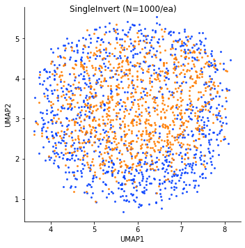
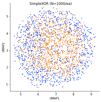
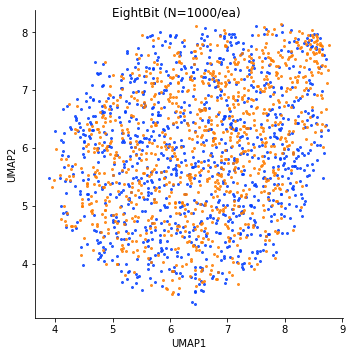
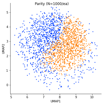
Figure 6: UMAP transform for the matching machine types of MLDS-DS1 and MLDS-DS2

Moving on to classification, we train several 2-class classifiers on machines from each dataset, the results of which are shown in Table 2. Each classifier is trained with 800 samples per class, and 200 samples are used for validation. These results mirror observed clustering results, with high accuracy in most classifiers for 4 out of 5 machine types, with SingleInvert being the notable exception that warrants further study.

Machine	SVM	DecisionTree	RandomForest	MLP	AdaBoost	NaiveBayes
EightBit	87%	78%	96%	91%	94%	99%
SingleDirect	96%	81%	95%	96%	99%	100%
SingleInvert	52%	49%	52%	53%	48%	55%
SimpleXOR	86%	85%	91%	85%	94%	99%
Parity	63%	55%	71%	66%	69%	61%

Table 2: 2-class classifier results for MLDS-DS1 (normal) or MLDS-DS2 (backdoor) networks, for N=1000 samples of each, 800 training, 200 validation

As in Section 4.2, the classifiers presented here are not tuned to this dataset. We are confident that better classification performance is possible with the results here serving as a baseline.

The results presented here show that, given enough examples, even a cursory meta-data analysis is sufficient to detect the small differences present in models with trojan backdoors.

5 Conclusions and Future Work

The dataset and analysis presented here is seen as a springboard for future research. As discussed in Section 3.3, there are number of new features planned for generating future datasets, including those based on standard feed forward networks, convolutional neural networks, and datasets that vary the network architecture as well as weights. Additionally, the analysis presented here on the existing dataset should be seen as a starting point for further research.

In this paper we introduce the MLDS dataset, a large collection of neural networks trained on similar data and designed to study weight-space analysis. It is generated using the novel MLC@Home distributed computing project, which opens new possibilities for ML research. Using this dataset, we show that weight-space analysis is useful in mapping a trained model back to its dataset and for detecting trojan networks without resorting to running examples through the network. We hope that this dataset forms the basis for a new path of research to understanding how neural networks represent what they learn.

Appendix A Details of Dataset Construction

The MLDS dataset consists of neural networks that mimic the behavior of simple machines. In this appendix we detail how the training data for each machine was created, how the random automata for MLDS-DS3 were created, and the PyTorch code for the individually trained networks.

A.1 Training Data Generation

Training data for each network is created by generating random input sequences for each machine and recording the resulting output sequence. We generate three separate datasets — one for training, one for validation, and a separate smaller set for evaluation back on the server. Table 3 shows the characteristics of each generated set.

The random sequences are straightforward for MLDS-DS1 and MLDS-DS3, MLDS-DS2 requires special handling as we need training data to reflect pathological cases that trigger the modified behavior. As such, we generate random input sequences as normal, and then insert the magic trigger sequences at random offsets within the sequence. Additionally, MLDS-DS2 has an extra evaluation set of solely pathological cases to test the accuracy of trained network.

Dataset	Sequence Length	Training	Validation	Evaluation
MLDS-DS1	1024	2048	512	64
MLDS-DS2	1024	2048	512	64*2
MLDS-DS3	256	4096	512	512

Table 3: Training set details for all three MLDS datasets

A.2 Random Automata Generation

MLDS-DS3 consists of networks which model machines based on randomly generated automata. The algorithm for generating these graphs is listed in Algorithm 1.

Result: A directed graph that represents a randomly-generated automaton

graph = create empty directed graph;

node_array = create N nodes;

shuffle(node_array);

mark emitter nodes;

for node in node_list do

       graph = add node;

      

end for

for node in node_list do

       edge_label = random_choice(alphabet);

       graph = add_edge(node, node+1, edge_label);

      

end for

for edge in graph do

       n1 = original node;

       n2 = destination node;

       for label in other entries in alphabet do

             new_dest = random choice(node in graph and not n2);

             graph = add_edge(n1, new_dest, label);

            

       end for

      

end for

Algorithm 1 Generates automaton from an alphabet, a number of states, and emitter states.

A.3 PyTorch Network Architecture

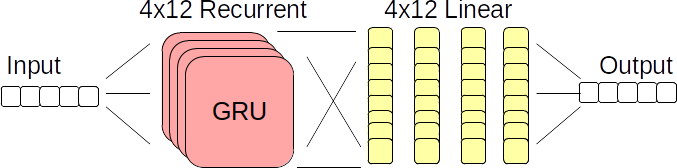
Figure 7: Network architecture for MLDS-DS1 and MLDS-DS2

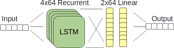
Figure 8: Network architecture for MLDS-DS3

MLDS-DS1/DS2 models each machine with a 4-layer deep GRU, followed by 4 fully-connected linear levels, with no activation functions between each layer. Each layer has a width of 12. Pseudo-code for this is shown in Figure 7. MLDS-DS3 uses exactly the same network, except with 4-layer stacked LSTM and 2 fully connected layers with no activation functions. However, each layer has a width of 64, leading to a significantly more complex network. The code for DS3 is the same as in Figure 8, but with LSTM instead of GRU.

References

- [1] David Anderson, Eric Korpela, and Rom Walton. High-performance task distribution for volunteer computing. In Proceedings - First International Conference on e-Science and Grid Computing, e-Science 2005, volume 2005, page 8 pp., 2006.
- [2] David P. Anderson. BOINC: A platform for volunteer computing. CoRR, abs/1903.01699, 2019.
- [3] Tom B. Brown, Dandelion Mané, Aurko Roy, Martín Abadi, and Justin Gilmer. Adversarial patch, 2018.
- [4] Kyunghyun Cho, Bart van Merrienboer, Caglar Gulcehre, Dzmitry Bahdanau, Fethi Bougares, Holger Schwenk, and Yoshua Bengio. Learning phrase representations using rnn encoder-decoder for statistical machine translation, 2014.
- [5] J. Clemens. Learning device models with recurrent neural networks. In 2018 International Joint Conference on Neural Networks (IJCNN), pages 1–8, 2018.
- [6] Tianyu Gu, Brendan Dolan-Gavitt, and Siddharth Garg. Badnets: Identifying vulnerabilities in the machine learning model supply chain, 2019.
- [7] Chuan Guo, Ruihan Wu, and Kilian Q. Weinberger. Trojannet: Embedding hidden trojan horse models in neural networks, 2021.
- [8] Sepp Hochreiter and Jürgen Schmidhuber. Long short-term memory. Neural Comput., 9(8):1735–1780, November 1997.
- [9] Kaggle: Your machine learning and data science community.
- [10] Kiran Karra, Chace Ashcraft, and Neil Fendley. The trojai software framework: An opensource tool for embedding trojans into deep learning models, 2020.
- [11] Diederik P. Kingma and Jimmy Ba. Adam: A method for stochastic optimization, 2017.
- [12] Leland McInnes, John Healy, and James Melville. Umap: Uniform manifold approximation and projection for dimension reduction, 2020.
- [13] Adam Paszke, Sam Gross, Francisco Massa, Adam Lerer, James Bradbury, Gregory Chanan, Trevor Killeen, Zeming Lin, Natalia Gimelshein, Luca Antiga, Alban Desmaison, Andreas Kopf, Edward Yang, Zachary DeVito, Martin Raison, Alykhan Tejani, Sasank Chilamkurthy, Benoit Steiner, Lu Fang, Junjie Bai, and Soumith Chintala. Pytorch: An imperative style, high-performance deep learning library. In H. Wallach, H. Larochelle, A. Beygelzimer, F. d'Alché-Buc, E. Fox, and R. Garnett, editors, Advances in Neural Information Processing Systems 32, pages 8024–8035. Curran Associates, Inc., 2019.
- [14] Frits Vaandrager. Model learning. Commun. ACM, 60(2):86–95, January 2017.
- [15] Xiaojun Xu, Qi Wang, Huichen Li, Nikita Borisov, Carl A. Gunter, and Bo Li. Detecting ai trojans using meta neural analysis, 2020.