Preheating and Reheating after Standard Inflation

Abstract

We study the two-phase scenario following inflation, where the initial step is preheating, accompanied by a step of perturbative reheating at which inflaton field decays transferring all of its energy to create relativistic particles, the interaction of these particles will evolve towards a state of thermal equilibrium with a temperature $T_{re}$ called the reheating temperature. It is observed that the scenario of reheating normally predicts the maximum reheating temperature that corresponds to an almost instantaneous transition from inflation to the radiation domination era. This will naturally lead to a nonperturbative preheating. In this framework, we propose constraints on the reheating duration parameters expressed in terms of the cosmic microwave background (CMB) inflationary scalar spectral index. In this work we study the compatibility of polynomial and Higgs models of inflation with the observational data obtained from Planck 2018.

1 Introduction

At the end of inflation, the universe enters a new stage, at which, the creation of elementary particles and its decay occurs. Note that, in the first phase, the creation of particles occurs due to parametric resonance called preheating, and in the last phase, the particles decay and thermalize with a final temperature called reheating temperature. The inflaton field $\phi$ starts oscillating near the minimum of its potential, with a decrease of the amplitude of the oscillations over time because the inflaton’s energy is transferred to other fields and relativistic particles. This is the mechanism of the production of elementary particles following inflation which we call reheating, the produced particles interact with each other until they reach a temperature of thermal equilibrium $T_{re}$.

At the stage of preheating[1], the field decay into bosons and because of the Pauli exclusion principle fermions production occurs only at the late stage of reheating, knowing that reheating at the parametric resonance stage is never complete, at the start the resonance was broad but eventually, it became narrow [2] then the reheating ends at the time of the thermalization of produced particles. In [4, 5] models of inflation considering instant reheating have been tested. We, therefore, will take into account the maximum reheating temperature that leads to the lower values of $N_{re}$ wich favor a much higher e-folds number of preheating, and prove that it’s parameterized by a post-inflationary e-folds $N_{pre}.$ The equation of state (eos) $\omega$ is an important parameter that can be used in the study of the evolution of the universe, the (eos) takes different values in each era of its history, for example, $\omega\geq-1/3$ is needed to end inflation[8, 9] but during the reheating the (eos) increase from $0$ to $1/3$, where $\omega=1/3$ corresponds to a universe of the radiation domination era[7].

2 Parametric resonance

The reheating process occurs when the inflaton energy density is transferred to the energy density of other fields, The decay rate of the inflaton oscillations parametrized with $\Gamma$[1], is added as a friction term to the motion equation given by  eq.(1)  which proves to be very useful in the study of reheating after inflation :

$$\ddot{\phi}+3H(t)\dot{\phi}+\Gamma\dot{\phi}+m^{2}\phi=0.$$ (2.1)

The solution of this equation from [11] suggested the concept that one can explain the effects of reheating using the total decay rate given by the formula $\Gamma=\Gamma(\phi\rightarrow\chi\chi)+\Gamma(\phi\rightarrow\overline{\psi}\psi)$, which describe the energy transferring to the new particles.

$$\phi(t)\approx\Phi(t)sin(m_{\phi}t),$$ (2.2)

$\phi(t)$ is the solution of the first equation, and $\Phi(t)$ is a decreasing amplitude that is in the form :

$$\Phi(t)=\Phi_{0}exp\left[-\dfrac{1}{2}(3H+\Gamma)t\right].$$ (2.3)

Preheating is the first stage of the reheating era, which is characterized by the appearance of $\phi$ and $\chi$ particles[1], which cannot be studied using perturbative theory[2]. Oscillations in the scalar field can decay into light $\chi$-particles, these particles are taken into account because of the interaction $\dfrac{1}{2}g^{2}\phi^{2}\chi^{2}$ which is given by the potential of the form

$$V(\phi,\chi)=\dfrac{1}{2}m_{\phi}^{2}\phi^{2}+\dfrac{1}{2}m_{\chi}^{2}\chi^{2}+\dfrac{1}{2}g^{2}\phi^{2}\chi^{2},$$ (2.4)

the time evolution of the quantum fluctuation of the field $\chi$ is given by

$$\ddot{\chi}+3H\dot{\chi}-\dfrac{1}{a^{2}}\nabla_{x}^{2}\chi+V^{{}^{\prime}}(\phi,\chi)=0,$$ (2.5)

deriving the potential with respect to $\chi$ and proceeding into Fourier space :

$$\ddot{\chi}_{k}+3H\dot{\chi_{k}}+\left(\dfrac{k^{2}}{a^{2}}+m_{\chi}^{2}+g^{2}\phi^{2}(t)\right)\chi_{k}=0,$$ (2.6)

according to[1] the above equation describes $\chi$-particles production by the excitation of the field, these particles have momentum $k/a\gg m_{\phi}$, knowing that the inflaton field only interacts with a light scalar field$\ \chi$ under the condition ($m_{\chi}\ll m_{\phi}$), taking in consideration the constant expansion of the universe $H\approx 0$, and using the solution in eq.19 with the condition that $\Phi$ is varying slowly compared to the oscillation of $\chi$-field[11], the eq.23 is reduced to :

$$\ddot{\chi}_{k}+\left(\dfrac{k^{2}}{a^{2}}+g^{2}\Phi^{2}sin^{2}(m_{\phi}t)\right)\chi_{k}=0,$$ (2.7)

using $z=mt$ and $sin^{2}(z)=1/2(1-cos(2z))$, we get the well known Mathieu equation :

$$\chi_{k}^{\prime\prime}+(A_{k}-2qcos(2z))\chi_{k}=0,$$ (2.8)

with $A_{k}=k^{2}/m^{2}+2q$, $q=g^{2}\Phi^{2}/4m^{2}$ and prime denote differentiation with respect to $z$. this equation describes an oscillator with a periodically changing frequency $\omega^{2}(t)=k^{2}+g^{2}\Phi^{2}sin(mt)$. As already mentioned, in the parametric resonance regime, the bosons were created due to the broad parametric resonance then the resonance became narrow. The broad resonance is known as the case were the parameter $q\gg 1$, and for $g\phi<m$ we have the narrow resonance with $q\ll 1$. An important feature of the solution of Mathieu equation is the existence of an exponential instability $\chi_{k}\propto exp(\mu_{k}z)$, this instability corresponds to an exponential growth of occupation number of quantum fluctuation $n_{k}(t)\propto exp(2\mu_{k}z)$[2].

3 Reheating duration

Information about reheating can be extracted considering the history of the Universe between inflation at which observed CMB modes crossed beyond the Hubble radius and the present time. Knowing that deferents eras occurred throughout this length of time that are parametrized by several e-folds numbers,

$$\dfrac{k}{a_{0}H_{0}}=\dfrac{a_{k}}{a_{end}}\dfrac{a_{end}}{a_{re}}\dfrac{a_{re}}{a_{eq}}\dfrac{a_{eq}H_{eq}}{a_{0}H_{0}}\dfrac{H_{k}}{H_{eq}}$$ (3.1)

$$ln\frac{k}{a_{0}H_{0}}=-N_{k}-N_{re}-N_{RD}+ln\frac{a_{eq}H_{eq}}{a_{0}H_{0}}+ln\frac{H_{0}}{a_{eq}}$$ (3.2)

here $k$ refers to the pivot scale for a specific experiment[7], and $N_{k}$ is the e-folds of the inflation era, $N_{re}$ and $N_{RD}$ respectively correspond to the reheating and radiation-domination era durations.

In addition to its thermalization temperature $T_{re}$ and equation of state $\omega_{re}$, reheating is also characterized by the number of e-folds $N_{re}=ln(a_{re}/a_{end})$ occurring between the time inflation ends, and the beginning of the radiation-dominated era, which we called the duration of reheating. Using $\rho\propto a^{-3(1+\omega_{re})}$, the reheating era can be described as :

$$\dfrac{\rho_{end}}{\rho_{re}}=\left(\dfrac{a_{end}}{a_{re}}\right)^{-3(1+\omega_{re})}$$ (3.3)

where $\rho_{end}$ and $a_{end}$ corresponds to the end of inflation and $\rho_{re}$ and $a_{re}$ corresponds to the end of reheating. We can re-write this using e-folds equation as

$$N_{re}=\dfrac{1}{3(1+\omega_{re})}ln\left(\dfrac{\rho_{end}}{\rho_{re}}\right),$$ (3.4)

and replace the energy densities by their expressions[7], $\rho_{end}=\dfrac{3}{2}V_{end}$ and $\rho_{re}=\dfrac{\pi^{2}}{30}g_{re}T_{re}^{4}$ in the previous equation to have :

$$N_{re}=\dfrac{1}{3(1+\omega_{re})}ln\left(\dfrac{3}{2}\dfrac{30V_{end}}{\pi^{2}g_{re}T_{re}^{4}}\right),$$ (3.5)

the conservation of the entropy between the end of reheating and the actual time can lead us to the assumption that reheating temperature and today temperature are related as[8] :

$$T_{re}=T_{0}\left(\dfrac{a_{0}}{a_{eq}}\right)e^{N_{RD}}\left(\dfrac{43}{11g_{re}}\right)^{1/3},$$ (3.6)

as a starting point, we will include the next equation

$$\dfrac{a_{0}}{a_{eq}}=\dfrac{a_{0}}{a_{k}}\dfrac{a_{k}}{a_{end}}\dfrac{a_{end}}{a_{re}}\dfrac{a_{re}}{a_{eq}},$$ (3.7)

the expression of the previous equation in terms of e-folds number will be given by :

$$\dfrac{a_{0}}{a_{eq}}=\dfrac{a_{0}H_{k}}{k}e^{-N_{k}}e^{-N_{re}}e^{-N_{RD}},$$ (3.8)

the expression of the temperature in the eq. (3.6) became :

$$T_{re}=\left(\dfrac{T_{0}a_{0}}{k}\right)H_{k}e^{-N_{k}}e^{-N_{re}}\left(\dfrac{43}{11g_{re}}\right)^{1/3},$$ (3.9)

replacing the previous equation in eq. (15) gives :

$$N_{re}=\dfrac{4}{1-3\omega_{re}}\left[\dfrac{1}{3}ln\left(\dfrac{11g_{re}}{43}\right)-ln\left(\dfrac{k}{a_{0}T_{0}}\right)-ln\left(\dfrac{V_{end}^{1/4}}{H_{k}}\right)-N_{k}\right].$$ (3.10)

Considering $g_{re}\approx 100$ and the pivot scale $0.05Mpc$ [7], the numerical application gives :

$$N_{re}=\dfrac{4}{1-3\omega_{re}}\left[6.61-ln\left(\dfrac{V_{end}^{1/4}}{H_{k}}\right)-N_{k}\right].$$ (3.11)

Now it is possible to calculate reheating duration as a function of the tree parameters $V_{end}$, $H_{k}$ and $N_{k}$ under the condition that $N_{re}$ is known. according to[10], the reheating ended at a temperature in the order of $10^{14}Gev$, if we used this result and applied it in eq.(15) we can find the reheating duration. Relating these parameters with the scalar spectral index $n_{s}$, and the choice of a specific inflation model with reheating (eos) $\omega_{re}$, will lead us to constrain reheating parameters in the standard inflation.

4 Reheating constraints in standard inflation

4.1 Standard infation

The main purpose of the theory of inflation is to solve the problems related to the Big-bang notably the horizon, flatness, and monopole problems. According to this theory, a scalar field called inflaton was responsible for an explosive phase that made the global geometry of the universe flat and made all regions of the universe connected causally. The evolution of the scalar field $\phi$ is described with the Klein-Gordon equation $\ddot{\phi}+3H\dot{\phi}+V^{\prime}(\phi)=0$. For a successful inflation, the slow-roll parameters given by $\epsilon=M_{p}^{2}V^{\prime 2}/2V^{2}$ and $\eta=M_{p}^{2}V^{\prime\prime}/V$ must obey the conditions $\epsilon<<1$ and $\eta<<1$.

Since the tree parameters $N_{k}$, $V_{end}$ and $H_{k}$ can be calculated as a function of the potential $V$ that can be related also to the slow-roll parameters, these parameters can be tested experimentally if we relate the slow-roll parameters to the scalar spectral index as described in the next equation:

$$n_{s}-1=-6\epsilon+2\eta$$ (4.1)

Once the form of $V(\phi)$ is specified for a given model, we can compute $N_{re}$ as a function of inflationary parameter $n_{s}$ for $\omega_{re}\in[-1/3,0]$

5 Polynomial potentials

Consider a polynomial potential

$$V=\dfrac{1}{2}m^{4-n}\phi^{n}.$$ (5.1)

We first need to calculate the parameters $N_{k}$, $H_{k}$, and $V_{end}$. The number of e-folds between the time the pivot scale exited the Hubble radius and the end of inflation is given by

$$N_{k}\simeq\dfrac{1}{M_{p}^{2}}\int_{\phi_{end}}^{\phi_{k}}\dfrac{V}{V^{\prime}}d\phi,$$ (5.2)

applying the previous equation to the polynomial potential :

$$N_{k}=\dfrac{1}{4nM_{p}^{2}}(\phi_{k}^{2}-\phi_{end}^{2}),$$ (5.3)

since $\phi_{end}$ is very small compared to the field at the beginning and during the inflation era, $\phi_{end}<<\phi_{k}$ it is appropriate to approximate

$$N_{k}\approx\dfrac{1}{4nM_{p}^{2}}\phi_{k}^{2},$$ (5.4)

we must write $N_{k}$ as a function of $n_{s}$ using the slow-roll parameters mentioned in the previous section and eq. (22) to obtain :

$$N_{k}=\dfrac{n+2}{2(1-n_{s})}.$$ (5.5)

Knowing that the Friedmann equation is written as :

$$H_{k}^{2}=\dfrac{1}{3M_{p}^{2}}V_{k},$$ (5.6)

$$r_{k}=\dfrac{2H_{k}^{2}}{\pi^{2}M_{p}^{2}A_{s}},$$ (5.7)

then using $r=16\epsilon_{k}$ gives

$$H_{k}=\pi M_{p}\sqrt{\dfrac{4nA_{s}}{n+2}(1-n_{s})},$$ (5.8)

and finally we can find $V_{end}$ [8] using

$$V_{k}=V_{end}\left(\dfrac{\phi_{k}}{\phi_{end}}\right)^{n}$$ (5.9)

to compute $V_{end}$ in terms of $n_{s}$ and $A_{s}$

$$V_{end}=\frac{12}{\sqrt{2}}\pi^{2}M_{p}^{4}A_{s}\left(\dfrac{n(1-n_{s})}{(n+2)}\right)^{n+2},$$ (5.10)

using $n_{s}=0.9649\pm 0.0042$ and Planck’s central value $\ln(10^{10}A_{s})=3.044$, we can plot the variations of $N_{re}$ as a function of $n_{s}$ for four different values of $\omega_{re}$ (see Figs. 1 and 2).

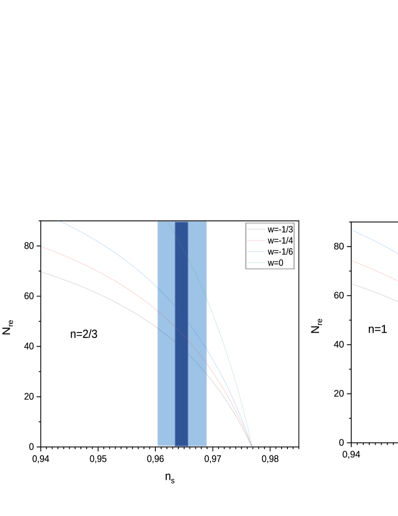
Figure 1: Variation of $N_{re}$ as function of $n_{s}$ for $n=2/3$ and $n=1$ for differentes values of $\omega_{re}$.

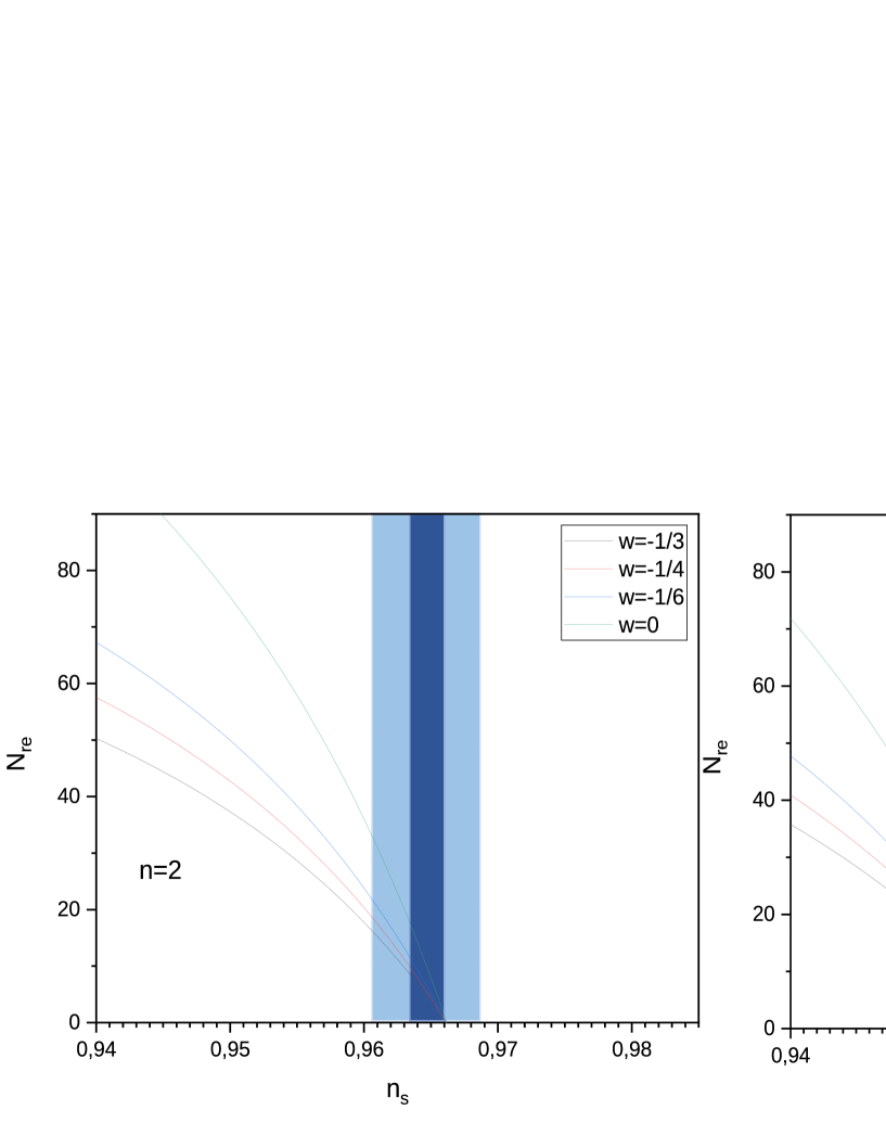
Figure 2: Variation of $N_{re}$ as function of $n_{s}$ for $n=2$ and $n=3$ for differentes values of $\omega_{re}$.

In Fig. 1 and 2, we apply the previous results to compute $N_{re}$ as functions of $n_{s}$. choosing the polynomial potential we study the reheating duration for several values of $n=2/3,1,2,3$. Moreover, we focus on reheating equation-of-state parameters in the interval $[-1/3,0]$. We plot $N_{re}$ as a function of $n_{s}$ for different values of the preheating equation-of-state parameters, in each case: $\omega_{re}=-1/3$ (black line), $\omega_{re}=-1/4$ (red line), $\omega_{re}=-1/6$ (blue line), and $\omega_{re}=0$ (green line).
We observe that for all four cases, all the lines with different values of $\omega_{re}$ converge to a central value where the preheating is instantaneous $N_{re}\rightarrow 0$, when we compared the results of the four cases we find that the chaotic model with $n=2$ is the most compatible with Planck’s $1\sigma$ bounds on $n_{s}$, but the case $n=3$ for all $\omega_{re}$ is difficult to reconcile in $1\sigma$ on $n_{s}$. As for the chaotic potential, the (eos) value$\ \omega_{re}\simeq 0\$is needed for an efficient reheating because it enables a much prolonged e-folds number of reheating.

6
Higgs potential

The Higgs inflation is based on the idea that the Higgs field is the inflaton field by adding a non-minimal coupling to gravity, the Higgs field potential is given by :

$$V=M_{p}^{4}\left(1-e^{-\phi\sqrt{2/3}/M_{p}}\right)^{2},$$ (6.1)

using this potential, one can calculate the number of e-foldings during inflation as :

$$N_{k}=\dfrac{1}{M_{p}}\int_{\phi_{end}}^{\phi_{k}}\dfrac{V}{V^{\prime}}d\phi=\dfrac{1}{2M_{p}^{2}}\sqrt{\dfrac{3}{2}}\left[M_{p}\sqrt{\dfrac{3}{2}}e^{\phi\sqrt{2/3}/M_{p}}-\phi\right]_{\phi_{end}}^{\phi_{k}}.$$ (6.2)

Knowing that the field obeys the condition $\phi_{k}\gg\phi_{end}$, and using the condition $M_{p}\sqrt{\dfrac{3}{2}}e^{\phi\sqrt{2/3}/M_{p}}\gg\phi_{k}$. the number of e-folds is simplified to

$$N_{k}=\dfrac{3}{4}e^{\phi\sqrt{2/3}/M_{p}},$$ (6.3)

which implies

$$\phi_{k}=\sqrt{\dfrac{3}{2}}M_{p}ln\left(\dfrac{4}{3}N_{k}\right),$$ (6.4)

using eq.(34) and the slow-roll parameters that are expressed by :

$$\epsilon_{k}\simeq\dfrac{3}{4N_{k}^{2}},\eta_{k}=-\dfrac{1}{N_{k}}$$ (6.5)

one must find the inflation e-folds which is given by

$$N_{k}=\dfrac{2}{1-n_{s}},$$ (6.6)

combining the expressions above, one derives $H_{k}$ and $V_{end}$ as function of $n_{s}$ and $A_{s}$ in the form :

$$H_{k}=\pi M_{p}\sqrt{\dfrac{3}{2}A_{s}}(1-n_{s})$$ (6.7)

and

$$V_{end}=\dfrac{9}{2}\pi^{2}M_{p}^{4}A_{s}(1-n_{s})^{2}\dfrac{\left(\dfrac{1}{\sqrt{3/2}+1}\right)^{2}}{\left(1-3/8)(1-n_{s})\right)^{2}}$$ (6.8)

All that remains now is to calculate the reheating duration for the case of Higgs inflation, taking in consideration the central values $n_{s}=0.9649\pm 0.0042$ and $\ln(10^{10}A_{s})=3.044$ according to Plank’s 2018 data.

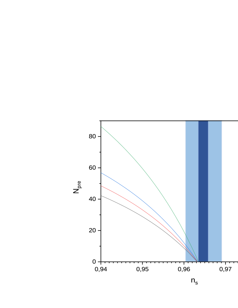
Figure 3: Variation of $N_{re}$ as function of $n_{s}$ in the case of Higgs inflation for $n=2/3$ and $n=1$ for differentes values of $\omega_{re}$.

The result in Figure 3 is a computation of $N_{re}$ as functions of $n_{s}$. Choosing the Higgs potential we study the reheating duration and focus on the same interval of (eos) parameters, We plot $N_{re}$ as a function of $n_{s}$.

The point where all the lines converge is considered to be the point of instantaneous reheating which is defined as the limit $N_{re}\rightarrow 0.$ We observe that for all different values of $\omega_{re}$ this model is compatible with the Planck $1\sigma$ bounds on $n_{s}$ because all the lines in this Figure are shifted toward the central value of $n_{s}$. Comparing this case with the chaotic inflation, the Higgs model (eos) parameter $\omega_{pre}\simeq 0\$is also required for an Efficient reheating since it allows a much prolonged duration of this stage.

7 Conclusion

In this work, we have calculated the reheating duration in the standard inflation for various cosmological parameters. We studied the preheating phase for the polynomial potential with the form $V\propto m^{4-n}\phi^{n}$ and the Higgs inflation. We showed that for the polynomial potential, the chaotic model with $n=2$ provides the best fit results with recent observational constraints because it’s compatible with Planck’s results, but the case $n=3$ shifted away from observation. The Higgs model shows good compatibility with Planck’s bounds of $n_{s}$. We finally concluded that for both potentials effecient reheating demand that $\omega_{re}\simeq 0$ which favors a much more post-inflationary e-folds of expansion for the reheating phase.

References

• [1] Kofman, L. A., Linde, A. D., & Starobinsky, A. A. (1985). Inflationary universe generated by the combined action of a scalar field and gravitational vacuum polarization. Physics Letters B, 157(5-6), 361-367.
• [2] Kofman, L., Linde, A., & Starobinsky, A. A. (1997). Towards the theory of reheating after inflation. Physical Review D, 56(6), 3258.
• [3] Aghanim, N., Akrami, Y., Ashdown, M., Aumont, J., Baccigalupi, C., Ballardini, M., … & Battye, R. (2018). Planck 2018 results. VI. Cosmological parameters. arXiv preprint arXiv:1807.06209.
• [4] Richar Easther, Hiranya V. Peiris. (2012).Β Bayesian analysis of inflation. II. Model selection and constraints on reheating. Physical Review D - Particles, Fields, Gravitation and Cosmology, 15507998.
• [5] Cuauhtemoc Campuzano and Sergio Del Campo, RamΓ³n Herrera. (2005). Curvaton reheating in tachyonic braneworld inflation.Β Physical Review D - Particles, Fields, Gravitation and Cosmology, 15507998.
• [6] Dmitry Podolsky, Gary N. Felder, Lev Kofman and Peloso Marco. (2006). Equation of state and beginning of thermalization after preheating. Physical Review D - Particles, Fields, Gravitation and Cosmology, 10.1103/PhysRevD.73.023501.
• [7] Cook, J. L., Dimastrogiovanni, E., Easson, D. A., & Krauss, L. M. (2015). Reheating predictions in single field inflation J. Cosmol. Astropart. Phys, 4(047), 1502-04673.
• [8] Dai, L., Kamionkowski, M., & Wang, J. (2014). Reheating constraints to inflationary models. Physical review letters, 113(4), 041302.
• [9] Kosar Asadi, Kourosh Nozari. Reheating constraints on a two-field inflationary model. Nuclear Physics B, 10.1016/j.nuclphysb.2019.114827.
• [10] Z. Sakhi, K. El Bourakadi, A. Safsafi, M. Ferricha-Alami H. Chakir, M. Bennai. Effect of brane tension on reheating parameters in small field inflation according to Planck-2018 data. International Journal of Modern Physics A, 10.1142/S0217751X20501912.
• [11] Allahverdi, R., Brandenberger, R., Cyr-Racine, F. Y., & Mazumdar, A. (2010). Reheating in inflationary cosmology: theory and applications. Annual Review of Nuclear and Particle Science, 60, 27-51.
• [12] Martin, J., Ringeval, C., Trotta, R., & Vennin, V. (2014). The best inflationary models after Planck. Journal of Cosmology and Astroparticle Physics, 2014(03), 039.