A note on some information-theoretic divergences
between Zeta distributions

Abstract

We consider the zeta distributions which are discrete power law distributions that can be interpreted as the counterparts of the continuous Pareto distributions with unit scale. The family of zeta distributions forms a discrete exponential family with normalizing constants expressed using the Riemann zeta function. We report several information-theoretic measures between zeta distributions and study their underlying information geometry.

1 Introduction

The zeta distributions [37, 27] are parametric discrete distributions with probability mass functions (PMFs) defined on the support of the natural integers $\mathbb{N}$ indexed by a scalar parameter $s\in(1,\infty)$ as follows:

$$p_{s}(x)=\Pr[X=x]\propto\frac{1}{x^{s}},\quad x\in\mathcal{X}=\mathbb{N}=\{1,2,\ldots\}.$$

The normalization function $\zeta(s)$ of the zeta distributions $p_{s}(x)=\frac{1}{\zeta(s)}\,\frac{1}{x^{s}}$ is the real Riemann zeta function [22, 69, 56, 33]:

$$\zeta(s)=\sum_{i=1}^{\infty}\frac{1}{i^{s}},\quad s>1.$$

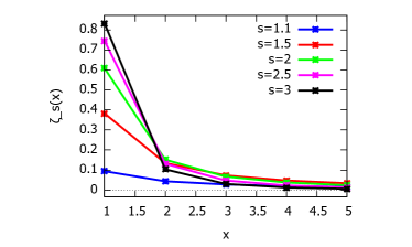
Figure 1: Several plots of the probability mass functions of zeta distributions.

Figure 1 displays several PMFs of zeta distributions. The zeta function can be bounded as follows [60] (see Figure 2):

$$\frac{1}{s-1}\leq\zeta(s)\leq\frac{s}{s-1}.$$ (1)

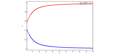
(a)	(b)

Figure 2: (a) Plot of the zeta function $\zeta(s)$ with its lower and upper bounds of Eq. 1. (b) Plots of the lower and upper bound gaps.

The set of zeta distributions $\mathcal{Z}=\{p_{s}(x)\ :\ s\in(1,\infty)\}$ forms a discrete exponential family [9] with natural parameter $\theta(s)=s$ lying in the natural parameter space $\Theta=(1,\infty)$, the sufficient statistic $t(x)=-\log x$, and the cumulant function or log-normalizer $F(\theta)=\log\zeta(\theta)$, a strictly convex and real analytic function (and hence $\zeta(s)$ is log-convex). Thus the pmf of zeta distributions can be rewritten in the canonical form of exponential families as:

$$p_{s}(x)=\exp\left(\theta(s)t(x)-F(\theta(s))\right).$$

The characteristic function is thus $\phi_{s}(t)=\frac{\zeta(s+it)}{\zeta(s)}$. An acceptance/rejection method to sample zeta variates is presented in Appendix B. Thus as an exponential family, the zeta distributions are maximum entropy discrete distributions for the constraint $-E[\log x]=\eta$ (a result formerly derived in [29]):

$$\max_{p}\left\{H(p)\quad:\quad-E_{p}[\log x]=\eta\Rightarrow p=\mathrm{Zeta}(\theta(\eta))\right\},$$

where $H(p)$ denotes the Shannon entropy of any distribution with full support $\mathbb{N}$:

$$H(p)=-\sum_{x\in\mathbb{N}}p(x)\log p(x).$$

We get the dual moment parameterization of a zeta distribution:

$$\eta(\theta)=F^{\prime}(\theta)=\frac{\zeta^{\prime}(\theta)}{\zeta(\theta)}.$$

A zeta distribution $p_{s}(x)$ can be interpreted as the discrete equivalent of a Pareto distribution $q_{s}(x)$ of scale $1$ and shape $s-1$ with probability density function $q_{s}(x)=\frac{s-1}{x^{s}}$ for $x>1$. See Table 1.

Table 1: Comparisons between the Zeta family and the Pareto subfamily. The function $\zeta(s)$ is the real zeta function.

	Zeta distribution	Pareto distribution
Exponential family $\exp(\theta t(x)-F(\theta))$
	Discrete EF	Continuous EF
PMF/PDF	$p_{s}(x)=\frac{1}{x^{s}\zeta(s)},\quad\zeta(s)=\sum_{i=1}^{\infty}\frac{1}{i^{s}}$	$q_{s}(x)=\frac{s-1}{x^{s}}$
Support $\mathcal{X}$	$\mathbb{N}=\{1,2,\ldots\}$	$(1,\infty)$
Natural parameter $\theta$	$s\in\Theta=(1,\infty)$	$s\in\Theta=(0,\infty)$
Cumulant $F(\theta)$	$\log\zeta(\theta)$	$-\log(\theta-1)$
Sufficient statistic $t(x)$	$-\log x$	$-\log x$
Moment parameter $\eta=-E[\log x]$	$\frac{\zeta^{\prime}(\theta)}{\zeta(\theta)}$	$-\frac{1}{s-1}$
Mean	$\frac{\zeta(s-1)}{\zeta(s)}$	$\frac{s}{s-1}$
Variance	$\frac{\zeta(s)\zeta(s-2)-\zeta(s-1)^{2}}{\zeta(x)^{2}},s>3$	$\frac{s}{(s-1)^{2}(s-2)},s>2$
Conjugate $F^{*}(\eta)$	$-H[p_{s}]=-\sum_{i=1}^{\infty}\frac{1}{i^{s}\zeta(s)}\log(i^{s}\zeta(s))$	$\eta-1-\log(-\eta)$
Maximum likelihood estimator	$\hat{\eta}=\frac{\zeta^{\prime}(\hat{\theta})}{\zeta(\hat{\theta})}=-\frac{1}{n}\sum_{i=1}^{n}\log x_{i}$	$\hat{s}=\frac{n}{\sum_{i=1}^{n}\log x_{i}}$
Fisher information	$\sum_{i=0}^{\infty}\Lambda(i)\log(i)i^{-s}$	$\frac{1}{(s-1)^{2}}$
Entropy $-F^{*}(\eta(s))$	$\sum_{i=1}^{\infty}\frac{1}{i^{s}\zeta(s)}\log(i^{s}\zeta(s))$	$1+\frac{1}{s-1}-\log(s-1)$
Bhattacharyya coefficient $I_{\alpha}$	$\frac{\zeta(\alpha s_{1}+(1-\alpha)s_{2})}{\zeta(s_{1})^{\alpha}\zeta(s_{2})^{1-\alpha}}$	$\frac{\alpha s_{1}+(1-\alpha)s_{2}}{s_{1}^{\alpha}s_{2}^{1-\alpha}}$
Kullback-Leibler divergence $D_{\mathrm{KL}}$	$\log(\zeta(s_{2}))-\sum_{i=1}^{\infty}\frac{1}{i^{s}\zeta(s)}\log(i^{s}\zeta(s))-s_{2}\frac{\zeta^{\prime}(s_{1})}{\zeta(s_{1})}$	$\log\left(\frac{s_{1}-1}{s_{2}-1}\right)+\frac{s_{2}-s_{1}}{s_{1}-1}$

The zeta function can be calculated fast [12, 30] and precisely [14, 34]. The derivatives of the zeta function have also been studied [74, 30]. In particular, for all even positive integer values, the zeta function $\zeta(2n)$ can be evaluated exactly using Bernoulli numbers $B_{2n}$ [28] (§6.5, p. 283): $\zeta(2n)=\frac{(-1)^{n+1}B_{2n}(2\pi)^{2n}}{2(2n)!},\quad n\in\mathbb{N}$. For example, we have $\zeta(2)=\frac{\pi^{2}}{6}$, $\zeta(4)=\frac{\pi^{4}}{90}$, $\zeta(6)=\frac{\pi^{6}}{945}$, etc.

The zeta distributions are related to the Zipf distributions [59, 61] $p_{s,N}(x)\propto\frac{1}{x^{s}}$ for $x\in\{1,\ldots,N\}$ and the Zipf-Mandelbrot distributions [40, 41, 39] $p_{s,q,N}(x)\propto\frac{1}{(x+q)^{s}}$ for $x\in\{1,\ldots,N\}$ which play an important role in quantitative linguistics. The Zipf distributions and the Zipf-Mandelbrot distributions both have finite support and can be interpreted as truncated zeta distributions (right truncation for Zipf distributions and both left & right truncations for the Zipf-Mandelbrot distributions) with normalizing constants which can be calculated approximately using properties of the zeta function [44]. Left-only truncations of the Zeta distributions are called Hurwitz zeta distributions [32]. Similarly, truncated Pareto distributions are used in applications [17]. Table 2 summarizes the terminology of truncated zeta distributions. Notice that truncated distributions of an exponential family with fixed truncation support form another exponential family [48]. Notice that the natural parameter space $\Theta$ of Zipf distributions is $(0,\infty)$ while the natural parameter space of zeta distributions is $(1,\infty)$ due to convergence requirements for the infinite zeta summation.

Table 2: Terminology for the truncated zeta distributions.

Left truncation	right truncation	distribution name
Yes	Yes	Zipf-Mandelbrot distribution [39]
Yes	No	Hurwitz zeta distribution [32]
No	Yes	Zipf distribution [61]

The zeta distributions and its related Hurwitz/Zipf/Zipf-Mandelbrot/distributions are discrete power law distributions which can be used to model the frequency of a word as a power law function of its frequency rank [7]. For example, the rank-frequency datasets of the translations of the Holy Bible in $100$ languages have been analyzed using the Zipf distributions in [42]. Zipf’s law occur empirically in many datasets where the ranked data exhibit the higher the fewer property (e.g., US firm sizes [5] or the surname frequencies [24]). The Zipf’s law is empirically only an approximation of a more complex distribution (see [43] for a study on the 30k english texts of the Project Gutenberg).

The zeta distributions are infinite divisible [32, 62, 18, 57]: A random variable following a zeta distribution can be expressed as the probability distribution of the sum of an arbitrary number of independent and identically distributed random variables. In applications, it is important to quantitatively discriminate between zeta distributions (see, for example [72, 55] or [20]). Mixtures of zeta distributions have also been used to model social networks [35]. In general, products of exponential families yield other exponential families. The products of $d$ zeta distributions form an exponential family called the Shintani multidimensional zeta distributions [4] or the zeta-star distributions [62].

We study information-theoretic divergences between zeta distributions by considering the fact that the set of zeta distributions form a discrete exponential family [10].

2 Amari’s $\alpha$-divergences and Sharma-Mittal divergences

To analyze sets of datasets exhibiting power law distributions, we may consider a notion of dissimilarity between discrete power law distributions. For example, a $100$ language translations of the Holy Bible was considered in [42] where each translation was analyzed by a Zipf distribution of the word rank-frequencies and characterized by the Zipf power exponent $s$ (see Table 1 in [42]). In order to cluster hierarchically or by $k$-means this set of (approximate) zeta distributions, we need to define a notion of distance between zeta distributions.

To measure the dissimilarity between two zeta distributions $p_{s_{1}}$ and $p_{s_{2}}$, one can use the $\alpha$-divergences [13] defined for a real $\alpha\in(0,1)$ as follows:

$$D_{\alpha}[p_{s_{1}}:p_{s_{2}}]:=\frac{1}{\alpha(1-\alpha)}\left(1-I_{\alpha}[p_{s_{1}}:p_{s_{2}}]\right),$$

where

$$I_{\alpha}[p_{1},p_{2}]:=\sum_{i=1}^{\infty}p_{1}(x)^{\alpha}p_{2}(x)^{1-\alpha},\quad\alpha\in(0,1)$$

is the $\alpha$-Bhattacharyya coefficient. The set of zeta distributions $\mathcal{E}:=\{p_{s}(x)\ :\ s\in(1,\infty)\}$ form a discrete exponential family [10] with natural parameter $\theta(s)=s$ (natural parameter space $\Theta=(1,\infty$), sufficient statistic $t(x)=-\log x$, and cumulant function $F(\theta)=\log\zeta(\theta)$ (see Table 1), a strictly convex and analytic function (see Figure 3): $p_{s}(x)=\exp\left(\theta(s)t(x)-F(\theta(s))\right)$.

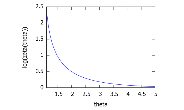
Figure 3: Plot of $F(\theta)=\log\zeta(\theta)$, a strictly convex and analytic function.

It follows from [50] that the skewed Bhattacharyya coefficient amounts to a skewed Jensen divergence between the natural parameters of the exponential family $\mathcal{E}$:

$$I_{\alpha}[p_{s_{1}}:p_{s_{2}}]=\exp\left(-J_{F,\alpha}(s_{1}:s_{2})\right),$$

where $J_{F,\alpha}$ is the skewed Jensen divergence induced by a strictly convex and smooth convex function $F(\theta)$:

$$J_{F,\alpha}(s_{1}:s_{2}) := \alpha F(s_{1})+(1-\alpha)F(s_{2})-F(\alpha s_{1}+(1-\alpha)s_{2})\geq 0,$$

$$= \log\left(\frac{\zeta(s_{1})^{\alpha}\zeta(s_{2})^{1-\alpha}}{\zeta(\alpha s_{1}+(1-\alpha)s_{2})}\right).$$

Thus we have the $\alpha$-divergences between two zeta distributions $p_{s_{1}}$ and $p_{s_{2}}$ available in closed-form.

Theorem 1 ($\alpha$-divergences between two zeta distributions)

The $\alpha$-divergence for $\alpha\in(0,1)$ between two zeta distributions $p_{s_{1}}$ and $p_{s_{2}}$ is:

$$D_{\alpha}[p_{s_{1}}:p_{s_{2}}]=\frac{1}{\alpha(1-\alpha)}\left(1-\frac{\zeta(\alpha s_{1}+(1-\alpha)s_{2})}{\zeta(s_{1})^{\alpha}\zeta(s_{2})^{1-\alpha}}\right).$$

It follows that when $s_{1}$, $s_{2}$, and $\alpha s_{1}+(1-\alpha)s_{2}$ are all positive even integers, we can evaluate exactly the $\alpha$-divergences between $p_{s_{1}}$ and $p_{s_{2}}$.

Example 1

Consider $s_{1}=4$ and $s_{2}=12$ with $\alpha=\frac{1}{2}$. The $\alpha$-divergence for $\alpha=\frac{1}{2}$ is the squared Hellinger divergence $D_{\frac{1}{2}}[p_{s_{1}},p_{s_{2}}]=\sum_{i=1}^{\infty}\left(\sqrt{p_{s_{1}}(i)}-\sqrt{p_{s_{2}}(i)}\right)^{2}$. Since $\alpha s_{1}+(1-\alpha)s_{2}=8$, we find the exact squared Hellinger divergence: $D_{\frac{1}{2}}[p_{4},p_{12}]=4\left(1-3\sqrt{\frac{715}{6910}}\right)\simeq 0.139929\ldots$.

Let us report another example where the squared Hellinger divergence is expressed using the zeta function:

Example 2

We consider $s_{1}=3$, $s_{2}=7$ and $\alpha=\frac{1}{2}$ so that $\alpha s_{1}+(1-\alpha)s_{2}=5$. Then we have $D_{\frac{1}{2}}[p_{3},p_{7}]=4\left(1-\frac{\zeta(5)}{\sqrt{\zeta(3)\zeta(7)}}\right)\simeq 0.23261\ldots$

Since $\lim_{\alpha\rightarrow 1}D_{\alpha}[p_{s_{1}}:p_{s_{2}}]=D_{\mathrm{KL}}[p_{s_{1}}:p_{s_{2}}]$ is the Kullback-Leibler divergence [13] (KLD) [50]

$$D_{\mathrm{KL}}[p_{s_{1}}:p_{s_{2}}]:=\sum_{i=1}^{\infty}p_{s_{1}}(i)\log\frac{p_{s_{1}}(i)}{p_{s_{2}}(i)},$$

we can approximate the KLD by $D_{1-\epsilon}[s_{1}:s_{2}]$ for a small value of $\epsilon$ (say, $\epsilon=1.0e^{-3}$) using fast methods to compute the zeta function [31]. Similarly, when $\alpha\rightarrow-1$, the $\alpha$-divergences tend to the reverse Kullback-Leibler divergence:

$$\lim_{\alpha\rightarrow-1}D_{\alpha}[p_{s_{1}}:p_{s_{2}}]=D_{\mathrm{KL}}[p_{s_{2}}:p_{s_{1}}]=D_{\mathrm{KL}}^{*}[p_{s_{1}}:p_{s_{2}}]=\sum_{i=1}^{\infty}p_{s_{2}}(i)\log\frac{p_{s_{2}}(i)}{p_{s_{1}}(i)}.$$

Corollary 1 (Approximation of the Kullback-Leibler divergence.)

The Kullback-Leibler divergence between two zeta distributions $p_{s_{1}}$ and $p_{s_{2}}$ can be approximated for small values $\epsilon>0$ by

$$D_{\mathrm{KL}}[p_{s_{1}}:p_{s_{2}}]\simeq D_{1-\epsilon}[p_{s_{1}}:p_{s_{2}}]=\frac{1}{\epsilon(1-\epsilon)}\left(1-\frac{\zeta((1-\epsilon)s_{1}+\epsilon s_{2})}{\zeta(s_{1})^{1-\epsilon}\zeta(s_{2})^{\epsilon}}\right).$$

We can also calculate the KLD $D_{\mathrm{KL}}[p_{s_{1}}^{\mathcal{X}_{1}}:p_{s_{2}}^{\mathcal{X}_{2}}]$ between two truncated zeta distributions with nested supports $\mathcal{X}_{1}\subseteq\mathcal{X}_{2}$. See [48]. A truncated zeta distribution on the support $\{a,a+1,\ldots,b\}\subset\mathbb{N}$ (with $b>a$) has pmf $p^{a,b}_{s}(x)=\frac{p_{s}(x)}{\Phi_{s}(b)-\Phi_{s}(a)}$ where $\Phi_{s}(u)$ is the cumulative distribution function $\Phi_{s}(u)=\sum_{x\in\{1,\ldots,u\}}p_{s}(x)=\frac{1}{\zeta(s)}\sum_{x\in\{1,\ldots,u\}}\frac{1}{x^{s}}$.

The Chernoff information [45] is defined by $C[p_{1},p_{2}]=-\log\min_{\alpha\in(0,1)}I_{\alpha}[p_{1},p_{2}]$. When both pdfs or pmfs belong to the same exponential family, we have [45]

$$C[p_{\theta_{1}},p_{\theta_{2}}]=J_{F}(\theta_{1}:(\theta_{1}\theta_{2})_{\alpha^{*}})=B_{F}(\theta_{1}:(\theta_{1}\theta_{2})_{\alpha^{*}})=B_{F}(\theta_{2}:(\theta_{1}\theta_{2})_{\alpha^{*}}),$$

where $B_{F}$ denotes the Bregman divergence (corresponding to the KLD) and $(\theta_{1}\theta_{2})_{\alpha^{*}}=\alpha^{*}\theta_{1}+(1-\alpha^{*})\theta_{2}$. For uniorder exponential family like the zeta distributions, we get a closed-form solution [45]:

$$\alpha^{*}=\frac{{F^{*}}^{\prime}(\Delta F/\Delta\theta)-\theta_{2}}{\Delta\theta},$$

where $\Delta\theta=\theta_{1}-\theta_{2}$, $\Delta F=F(\theta_{1})-F(\theta_{2})$, an $F^{*}(\eta)$ is the convex conjugate of $F(\theta)$. For example, applying this formula for the Pareto distributions with $s_{1}\not=s_{2}$ and ${F^{*}}^{\prime}(\eta)=1-\frac{1}{\eta}$, we get

$$\alpha^{*}=\frac{1-s_{2}}{s_{1}-s_{2}}-\frac{1}{\log\frac{s_{2}-1}{s_{1}-1}},$$

and the Chernoff information between two Pareto distributions is

$$C[p_{s_{1}},p_{s_{2}}]=\log\frac{s_{1}^{\alpha^{*}}s_{2}^{1-\alpha^{*}}}{\alpha^{*}s_{1}+(1-\alpha^{*})s_{2})}.$$

The information geometry (i.e., the Fisher-Rao manifold, the dual $\alpha$-connections, and the Jeffreys’ prior) of the Pareto distributions has been studied in [1, 67, 38]. The biparametric family of Pareto distributions $\{p_{s,a}(x)=(s-1)\frac{a^{s-1}}{x^{s}},s>1,a>0\}$ equipped with the Fisher information metric yields a manifold of positive curvature [1, 58] (and thus this contrasts with the manifolds of location-scale families which are always of non-positive curvature).

The Sharma-Mittal divergences [65] between two densities $p$ and $q$ is a biparametric family of relative entropies is defined by

$$D_{\alpha,\beta}[p:q]=\frac{1}{\beta-1}\left(\left(\int p(x)^{\alpha}q(x)^{1-\alpha}\mathrm{d}x\right)^{\frac{1-\beta}{1-\alpha}}-1\right),\forall\alpha>0,\alpha\neq 1,\beta\neq 1.$$

The Sharma-Mittal divergence is induced from the Sharma-Mittal entropies which unifies the extensive Rényi entropies with the non-extensive Tsallis entropies [65]. The Sharma-Mittal divergences include the Rényi divergences ($\beta\rightarrow 1$) and the Tsallis divergences ($\beta\rightarrow\alpha$), and in the limit case of $\alpha,\beta\rightarrow 1$ the Kullback-Leibler divergence [52]. When both densities $p=p_{\theta_{1}}$ and $q=p_{\theta_{2}}$ belong to the same exponential family, we have the following closed-form formula [52]:

$$D_{\alpha,\beta}[p_{\theta_{1}}:p_{\theta_{2}}]=\frac{1}{\beta-1}\left(e^{-\frac{1-\beta}{1-\alpha}J_{F,\alpha}\left(\theta_{1}:\theta_{2}\right)}-1\right).$$

Thus we get the following theorem:

Theorem 2

For $\alpha>0$, $\alpha\not=1$, $\beta\not=1$, the Sharma-Mittal divergence between two zeta distributions $p_{s_{1}}$ and $p_{s_{2}}$ is

$$D_{\alpha,\beta}[p_{s_{1}}:p_{s_{2}}]=\frac{1}{\beta-1}\left(\left(\frac{\zeta(\alpha s_{1}+(1-\alpha)s_{2})}{\zeta(s_{1})^{\alpha}\zeta(s_{2})^{1-\alpha}}\right)^{\frac{1-\beta}{1-\alpha}}-1\right).$$

3 The Kullback-Leibler divergence between two zeta distributions

It is well-known that the KLD between two probability mass functions of an exponential family amounts to a reverse Bregman divergence induced by the cumulant function [6]: $D_{\mathrm{KL}}[p_{s_{1}}:p_{s_{2}}]=B_{F}^{*}(\theta_{1}:\theta_{2}):=B_{F}(\theta_{2}:\theta_{1})$ (with $\theta_{1}=s_{1}$ and $\theta_{2}=s_{2}$). Furthermore, this Bregman divergence $B_{F}$ amounts to a Fenchel-Young divergence $Y_{F,F^{*}}$ [47] so that we have

$$D_{\mathrm{KL}}[p_{s_{1}}:p_{s_{2}}]=B_{F}(\theta_{2}:\theta_{1})=F(\theta(s_{2}))+F^{*}(\eta(s_{1}))-\theta(s_{2})\eta(s_{1}):=Y_{F,F^{*}}(\theta(s_{2}):\eta(s_{1})),$$

where $F^{*}(\eta)$ denotes the Legendre convex conjugate of $F$, $\theta(s)=s$ and $\eta(s)=F^{\prime}(\theta(s))=E_{p_{s}}[t(x)]=-E_{p_{s}}[\log x]$, see [9]. Moreover, the convex conjugate $F^{*}(\eta(s))$ corresponds to the negentropy [51]: $F^{*}(\eta(s))=-H[p_{s}]$, where the entropy of a zeta distribution $p_{s}$ is defined by:

$$H[p_{s}]:=\sum_{i=1}^{\infty}p_{s}(i)\log\frac{1}{p_{s}(i)}.$$

Using the fact that $\sum_{i=1}^{\infty}p_{s}(i)=1=\sum_{i=1}^{\infty}\frac{1}{i^{s}\zeta(s)}$, we can express the entropy as follows:

$$H[p_{s}] = \sum_{i=1}^{\infty}\frac{1}{i^{s}\zeta(s)}\log i^{s}+\log(\zeta(s))\sum_{i=1}^{\infty}\frac{1}{i^{s}\zeta(s)},$$

$$= \sum_{i=1}^{\infty}\frac{1}{i^{s}\zeta(s)}\log(i^{s}\zeta(s)).$$

Since $F(\theta)=\log\zeta(\theta)$, we have $\eta(\theta)=F^{\prime}(\theta)=\frac{\zeta^{\prime}(\theta)}{\zeta(\theta)}$. The function $\frac{\zeta^{\prime}(\theta)}{\zeta(\theta)}$ has been tabulated in [71] (page 400). Notice that the maximum likelihood estimator [10, 11] (MLE) of $n$ identically and independently (iid.) observations $x_{1},\ldots,x_{n}$ is

$$\max_{s}\frac{1}{n}\sum_{i=1}^{n}\log p_{s}(x_{i})=\max_{s}-\frac{1}{n}\sum_{i=1}^{n}\log x_{i}-\log\zeta(s).$$

Thus we get [64].

$$\hat{\eta}=\frac{\zeta^{\prime}(\hat{\theta})}{\zeta(\hat{\theta})}=-\frac{1}{n}\sum_{i=1}^{n}\log x_{i}.$$

See [17] for the MLE of the truncated Pareto distributions.

Remark 1

The Cramér-Rao lower bound (CRLB) states that the variance of any unbiased estimator $\hat{s}$ is greater or equal than the inverse of the Fisher information. Let $X=(X_{1},\ldots,X_{n})\sim_{\mathrm{iid}}\mathrm{Zeta}(s)$. Then $I_{X}=nI(s)$ and we have the CRLB:

$$\mathrm{Var}[\hat{s}]\geq\frac{1}{n}I^{-1}(s)=\frac{\zeta^{2}(s)}{n(\zeta(s)\zeta^{\prime\prime}(s)-\zeta^{\prime}(s)^{2})}.$$

This is in accordance with Section 2 of [21]. Moreover, the unbiased MLE matches exactly this bound only when dealing with exponential families [68].

The inverse of the zeta function $\zeta^{-1}(\cdot)$ has been studied in [36]. An alternative estimator of the zeta parameter (called the quadratic distance estimator, QDE) has been proposed in [21]: We consider the vector $X=\left(\log\frac{1}{2},\ldots,\log\frac{N-1}{N}\right)$ and the vector of log frequency ratio $Y=\left(\log\frac{f_{2}}{f_{1}},\ldots\log\frac{f_{N}}{f_{N-1}}\right)$ (where $f_{i}=\frac{n_{i}}{n}$ denotes the frequency of the $i$th item, the ratio of occurences of the $i$th item over the total number of items), and write the system of equations $Y=sX+(\epsilon_{1},\ldots,\epsilon_{N-1})$. Thus the QDE amounts to a mere line fitting procedure. See also [15].

Proposition 1 (KLD between zeta distributions)

The Kullback-Leibler divergence between two zeta distributions can be written as:

$$D_{\mathrm{KL}}[p_{s_{1}}:p_{s_{2}}] = \log(\zeta(s_{2}))-H[p_{s_{1}}]+s_{2}E_{p_{s_{1}}}[\log x],$$

$$= \log(\zeta(s_{2}))-\sum_{i=1}^{\infty}\frac{1}{i^{s_{1}}\zeta(s_{1})}\log(i^{s_{1}}\zeta(s_{1}))-s_{2}\frac{\zeta^{\prime}(s_{1})}{\zeta(s_{1})}.$$

Moreover, the logarithmic derivative of the zeta function can be expressed using the von Mangoldt function [73] (page 1850) for $\theta>1$:

$$\eta(\theta)=\frac{\zeta^{\prime}(\theta)}{\zeta(\theta)}=-\sum_{i=1}^{\infty}\frac{\Lambda(i)}{i^{\theta}},$$

where $\Lambda(i)=\log p$ is $i=p^{k}$ for some prime $p$ and integer $k\geq 1$ and $0$ otherwise:

$$\Lambda(i)=\begin{cases}\log p&\text{if }i=p^{k}\text{ for some prime }p\text{ and integer }k\geq 1,\\ 0&\text{otherwise.}\end{cases}$$

Figure 4 displays a plot of the von Mangoldt function. The von Mangoldt function satisfies the following identity:

$$\log(n)=\sum_{i|n}\Lambda(i),$$

where $i|n$ means $i$ divides $n$.

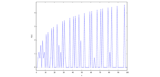
Figure 4: Plot of the von Mangoldt function in the range $\{1,\ldots,100\}$.

Notice that the zeta function can be calculated using Euler product formula: $\zeta(\theta)=\prod_{p:\mathrm{prime}}\frac{1}{1-p^{-\theta}}$.

Theorem 3

The Kullback-Leibler divergence between two zeta distributions can be expressed using the real zeta function $\zeta$ and the von Mangoldt function $\Lambda$ as:

$$D_{\mathrm{KL}}[p_{s_{1}}:p_{s_{2}}]=\log(\zeta(s_{2}))-\sum_{i=1}^{\infty}\frac{1}{i^{s}\zeta(s)}\log(i^{s}\zeta(s))+s_{2}\sum_{i=1}^{\infty}\frac{\Lambda(i)}{i^{s_{1}}}.$$

Example 3

Consider $s_{1}=4$ and $s_{2}=12$. Letting $\epsilon=0.9999$ and using Corollary 1, we get

$$D_{\mathrm{KL}}[p_{s_{1}}:p_{s_{2}}]\simeq D_{1-\epsilon}[p_{s_{1}}:p_{s_{2}}]=0.430479743738878\ldots$$

Let us now calculate the KLD using Theorem 3, we get $\log(\zeta(s_{2}))=\log\frac{691\pi^{1}2}{638512875}$, $H[p_{s_{1}}]\simeq 0.3337829096182664\ldots$ (using $100$ terms), and $\eta(s_{1})=-0.06366938697034288\ldots$ (using $100$ terms) so that we have

$$D_{\mathrm{KL}}[p_{s_{1}}:p_{s_{2}}] = \log(\zeta(s_{2}))-\sum_{i=1}^{\infty}\frac{1}{i^{s}\zeta(s)}\log(i^{s}\zeta(s))+s_{2}\sum_{i=1}^{\infty}\frac{\Lambda(i)}{i^{s_{1}}},$$ (2)

$$\simeq 0.430495790304827\ldots$$ (3)

It is well-known that the KLD between two arbitrarily close zeta distributions $p_{s}$ and $p_{s+\mathrm{d}s}$ amounts to half of the quadratic distance induced by the Fisher information:

$$D_{\mathrm{KL}}[p_{s}:p_{s+\mathrm{d}s}]\approx\frac{1}{2}I(s)\mathrm{d}s^{2},$$

where

$$I(s)=E_{p_{s}}[{(\log p_{s}(x))^{\prime}}^{2}]=-E_{p_{s}}[(\log p_{s}(x))^{\prime\prime}],$$

where the first-order and second-order derivatives are taken with respect to the parameter $s$. Thus for uniorder exponential families, the Fisher information matrix is

$$I(s)=-E_{p_{s}}[(\log p_{s}(x))^{\prime\prime}]=(\log\zeta(s))^{\prime\prime}=\frac{\zeta(s)\zeta^{\prime\prime}(s)-\zeta^{\prime}(s)^{2}}{\zeta^{2}(s)}.$$

This second-order derivative $(\log\zeta(s))^{\prime\prime}$ has been studied in [66]: Near $s=1$, we have

$$(\log\zeta(s))^{\prime\prime}=\frac{1}{(s-1)^{2}}+O(1),$$

and this coincides with the FIM of the Pareto distribution (see Table 1). We have

$$I(s)=\sum_{n=1}^{\infty}\Lambda(n)\log(n)n^{-s}$$

where $\Lambda(n)$ is the von Mangoldt function.

4 Comparison of the Zeta family with a Pareto subfamily

The zeta distribution is also called the “pure power-law distribution” is in the literature [27].

We can compute the $\alpha$-divergences between two Pareto distributions $q_{s_{1}}$ and $q_{s_{2}}$ with fixed scale $1$ and respective shapes $s_{1}-1$ and $s_{2}-1$. In our case, the Pareto density writes $q_{s}(x)=\frac{s-1}{x^{s}}$ for $x\in\mathcal{X}=(1,\infty)$. The family of such Pareto distributions forms a continuous exponential family with natural parameter $\theta=s$, sufficient statistic $t(x)=-\log(x)$, and convex cumulant function $F(\theta)=-\log(\theta-1)$ for $\theta\in\Theta=(1,\infty)$. Thus we have [50]:

$$I_{\alpha}[q_{1}:q_{2}]=\int q_{s_{1}}(x)^{\alpha}q_{s_{2}}(x)^{1-\alpha}\mathrm{d}x = \exp(-J_{F,\alpha}(\theta_{1}:\theta_{2})),$$

$$= \frac{\alpha s_{1}+(1-\alpha)s_{2}}{s_{1}^{\alpha}s_{2}^{1-\alpha}},$$

and we get the following closed-form for the $\alpha$-divergences between two Pareto distributions $q_{s_{1}}$ and $q_{s_{2}}$:

$$D_{\alpha}[q_{s_{1}}:q_{s_{2}}]=\frac{1}{\alpha(1-\alpha)}\left(1-\frac{\alpha s_{1}+(1-\alpha)s_{2}}{s_{1}^{\alpha}s_{2}^{1-\alpha}}\right).$$

The moment parameter is $\eta(\theta)=F^{\prime}(\theta)=-\frac{1}{\theta-1}$ so that $\theta(\eta)=1-\frac{1}{\eta}$ and $F^{*}(\eta)=\theta(\eta)\eta-F(\theta(\eta))=\eta-1-\log(-\eta)$. It follows that the KLD is

$$D_{\mathrm{KL}}[q_{s_{1}}:q_{s_{2}}]=B_{F}(\theta_{2}:\theta_{1})=\log\left(\frac{s_{1}-1}{s_{2}-1}\right)+\frac{s_{2}-s_{1}}{s_{1}-1}.$$

The differential entropy of the Pareto distribution $q_{s}$ is

$$h[q_{s}]=-\int_{1}^{\infty}q_{s}(x)\log q_{s}(x)\mathrm{d}x=-F^{*}(\eta(s))$$

with $\eta(s)=-\frac{1}{s-1}$. We find that

$$h[q_{s}]=1+\frac{1}{s-1}-\log(s-1).$$

The Pareto distributions form a discrete exponential family and are thus maximum entropy distributions under the moment constraints $-E[\log x]=\eta$:

$$\max\left\{h(q)\quad:\quad E[\log x]=-\eta\right\}.$$

The differences with the Zeta distribution is that the support is considered $(1,\infty)$ instead of $\mathbb{N}$ and that the entropy is the differential entropy instead of the discrete entropy. Notice that the differential entropy may be negative (e.g., for the Pareto distributions when $s$ is large) but never the discrete entropy.

Example 4

For comparison, we calculate the KLD between two Pareto distributions with parameters $s_{1}=4$ and $s_{2}=12$. We find

$$D_{\mathrm{KL}}[q_{s_{1}}:q_{s_{2}}]=\log\frac{3}{11}+\frac{8}{3}\simeq 1.367383682536406\ldots$$

Table 1 compares the discrete exponential family of zeta distributions with the continuous exponential family of Pareto distributions with fixed scale $1$.

Since the information-theoretic distances between zeta distributions are computationally demanding, one can also investigate both fast(er) lower and upper bounds on these distances. Bounds on the $f$-divergences (including the $\alpha$-divergences) between Zipf-Mandelbrot distributions have been studied in [39, 2].

In general, it is interesting to consider discrete counterparts of continuous exponential families. For example, the discrete Gaussian distributions or discrete normal distributions defined as maximum entropy distributions have been studied in [3, 49]. The log-normalizer or cumulant function of the discrete Gaussian distributions are related to the Riemann theta function [16]. Given a prescribed sufficient statistics $t(x)$, we may define the continuous exponential family wrt the Lebesgue measure $\mu$ as the probability density functions $p(x)$ maximizing the differential entropy under the moment constraint $E_{p}[t(x)]=\eta$. The corresponding discrete exponential family is obtained by the distributions with probability mass functions maximizing Shannon entropy under the moment constraint $E_{p}[t(x)]=\eta$. Notice that the raw (uncentered) moments $\mu_{k}$ of the zeta distributions are

$$\mu_{k}=E[X^{k}]=\frac{1}{\zeta(s)}\sum_{i=1}^{\infty}\frac{1}{i^{s-k}}=\left\{\begin{matrix}\zeta(s-k)/\zeta(s)&\textrm{for}~{}k<s-1\\ \infty&\textrm{for}~{}k\geq s-1\end{matrix}\right.$$

5 Clustering finite sets of Zipf’s distributions

Consider a finite set $\mathcal{P}=\{p_{\theta_{1},N_{1}},\ldots,p_{\theta_{n},N_{n}}\}$ of $n$ Zipf’s distributions with corresponding discrete supports $\mathcal{X}_{1}=\{1,\ldots,N_{1}\},\ldots,\mathcal{X}_{n}=\{1,\ldots,N_{n}\}$. For example, to fix ideas, we may consider the set of $100$ Zipf’s distributions obtained by analyzing the word frequency of translations of the Holy bible (see Table 1 of [42] with a short excerpt displayed in Table 3). Each translation in a natural language uses a vocabulary of $N$ distinct words and is modeled by a Zipf distribution $p_{\theta,N}$. These Zipf’s distributions somehow characterize some intrinsic properties of natural languages [23], and we may cluster these Zipf’s distributions to interpret how corresponding languages are similar [25] or not. We may cluster either using the agglomerative hierarchical clustering or partition-based $k$-means or $k$-centers algorithms [46].

Table 3: Some parameters $\theta>0$ of Zipf’s distributions obtained as word ranking-frequency distributions of the Holy Bible translations. Data excerpt extracted from Table 1 of [42].

Natural language	$\theta$	N
English	1.258	12702
French	1.161	24716
Japanese	0.774	30785
Danish	1.158	26290
Chinese	0.792	1699
Finnish	0.997	54863
…	…	…

Consider the $k$-means algorithm which partitions $\mathcal{P}=\uplus_{i=1}^{k}\mathcal{P}_{i}$ into $k$ pairwise disjoint subsets, with each subset $\mathcal{P}_{j}$ summarized by a zeta prototype distribution $q_{s_{j}}$ with full support $\mathbb{N}$. Lloyd’s heuristic of $k$-means consists in iteratively associating to each Zipf’s distribution $p_{\theta_{i},N_{i}}$ its closest zeta distribution $q_{s_{j}}$ with respect to the Kullback-Leibler divergence, and then update the cluster zeta distribution prototypes by taking their cluster centroids with respect to the Kullback-Leibler divergence. This clustering algorithm yields is an extension of the Bregman $k$-means algorithm [8] once the KLD between a Zipf’s distribution $p_{\theta,N}$ (i.e., a truncated zeta distribution) and a zeta distribution $q_{s}$ is identified to a duo Bregman divergence [48]:

$$D_{\mathrm{KL}}[p_{\theta,N}:q_{s}]=B_{F_{2},F_{1}}(s:\theta)=F_{2}(s)-F_{1}(\theta)-(s-\theta)F_{1}^{\prime}(\theta),$$ (4)

where $F_{2}(s)=\log\zeta(s)$, $F_{1}(\theta)=\log H_{N,\theta}$ where

$$H_{N,\theta}=\sum_{i=1}^{N}\frac{1}{i^{\theta}}$$

denotes the generalized harmonic number with

$$F_{1}^{\prime}(\theta)=\frac{H_{N,\theta}^{\prime}}{H_{N,\theta}}=-\sum_{i=1}^{N}\frac{\log i}{i^{\theta}\,H_{N,\theta}}.$$

Figure 5 displays two PMFs of Zipf’s distributions with different supports. The set of Zipf’s distribution with fixed support $\{1,\ldots,N\}$ form an exponential family $\mathcal{E}_{N}$, and thus the set of all Zipf exponential families $\cup_{N=1}^{\infty}\mathcal{E}_{N}$ form a “foliated exponential family” (like the set of Weibull distributions with shape parameter $k$ in $\{1,\ldots\}$ form another foliated exponential family) with the exponential family of zeta distributions in the limit case $N\rightarrow\infty$.

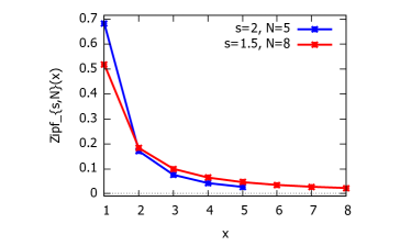
Figure 5: Two probability mass functions of Zipf’s distribution with different supports.

Thus the KLD between a Zipf distribution $p_{\theta,N}$ and a zeta distribution $q_{s}$ can be calculated in closed-form using Eq. 4:

$$D_{\mathrm{KL}}[p_{\theta,N}:q_{s}]=\log\frac{\zeta(s)}{\sum_{i=1}^{N}\frac{1}{i^{\theta}}}+(s-\theta)\sum_{i=1}^{N}\frac{\log i}{i^{\theta}\,H_{N,\theta}}.$$ (5)

Remark 2

More generally, we may consider two truncated zeta distributions $q_{s_{1}}^{a_{1},b_{1}}(x)=\frac{1}{x^{s_{1}}\zeta^{a_{1},b_{1}}(s_{1})}$ and $q_{s_{1}}^{a_{2},b_{2}}=\frac{1}{x^{s_{1}}\zeta^{a_{2},b_{2}}(s_{2})}$ with $\zeta^{a,b}(s)=\sum_{i=a}^{b}\frac{1}{x^{s}}$. When $[a_{1},b_{1}]\subseteq[a_{2},b_{2}]$, we may apply formula Eq. 4 with $F_{1}(s)=\log\zeta^{a_{1},b_{1}}(s)$ and $F_{2}(s)=\log\zeta^{a_{2},b_{2}}(s)$.

Lloyd’s heuristic minimizes the following energy:

$$\sum_{i=1}^{n}\min_{j\in\{1,\ldots,k\}}D_{\mathrm{KL}}[p_{\theta_{i}}:s_{j}]=\sum_{i=1}^{n}\min_{j\in\{1,\ldots,k\}}B_{F_{2},F_{1}}(s_{j}:\theta_{i}).$$

To calculate the cluster prototype $p_{s_{i}}$ corresponding to cluster $\mathcal{P}_{i}$, we need to solve the following generic optimization problem:

$$\min_{s\in(0,\infty)}\sum_{p_{\theta,N}\in\mathcal{P}_{i}}D_{\mathrm{KL}}[p_{\theta,N}:q_{s}]=\min_{s\in(0,\infty)}\sum_{p_{\theta,N}\in\mathcal{P}_{i}}B_{F_{2},F_{1}}(s:\theta).$$

We get $\eta_{s}:=\frac{\zeta^{\prime}(s)}{\zeta(s)}=\frac{1}{|\mathcal{P}_{i}|}\sum_{p_{N,\theta}\in\mathcal{P}_{i}}\frac{H_{N,\theta}^{\prime}}{H_{N,\theta}}$. Notice that we can also cluster just by a careful initialization using $k$-means++ [70] extended to any arbitrary divergence [54] (here a duo Bregman divergence). However, although the prototype distributions $q_{s_{i}}$ are parameterized by a single parameter $s_{i}$, we cannot use the optimal interval clustering relying on dynamic programming [53] since the supports $\mathcal{X}_{1},\ldots,\mathcal{X}_{n}$ may be different, and the clusters in the optimal $k$-means may have disjoint intervals.

Remark 3

When all Zipf’s distributions have coinciding support $\mathcal{X}$, we get the interval clustering property of $k$-means (since in that case, Bregman Voronoi diagrams have connected cells) and may use the optimal dynamic programming algorithm [53].

We may also consider the Bhattacharyya distance between two Zipf’s distributions $p_{\theta_{i},N_{i}}$ and $p_{\theta_{j},N_{j}}$ by considering the common support $\{1,\ldots,\min\{N_{i},N_{j}\}\}$:

$$D_{\mathrm{Bhat}}[p_{\theta_{i},N_{i}}:p_{\theta_{i},N_{i}}]=-\log\sum_{x=1}^{\min\{N_{i},N_{j}\}}\sqrt{p_{\theta_{i},N_{i}}(x)\,p_{\theta_{j},N_{j}}(x)}.$$

We get a duo Jensen divergence (see Theorem 2 of [48]).

Yet another approach is to convert the Zipf’s distributions $p_{N_{i},s_{i}}$ into Zeta distributions $p_{s_{i}}$. This conversion is motivated by Seal [63]’s estimator of the parameter of a Zeta distribution from an iid random sample of size $n$:

$$\hat{s}_{\mathrm{Seal}}=\frac{\log\frac{f_{1}}{f_{2}}}{\log 2},$$

where $f_{i}=\frac{n_{i}}{n}$ denotes the $i$-th highest frequency. Since $\frac{f_{1}}{f_{2}}=2^{s}$ for the zeta distribution, we get $\hat{s}_{\mathrm{Seal}}=s$. This estimator has variance $\mathrm{Var}[\hat{s}_{\mathrm{Seal}}]=\frac{\zeta(s)(1+2^{s})}{n\log^{2}2}$.

Appendix A Code snippets in Maxima

We give below some code snippets in Maxima (https://maxima.sourceforge.io/) to numerically calculate the examples reported in this technical report.

Code snippet 1

PMFzeta(x,s):=1.0/((x**s)*zeta(s));
s1:4;
s2:12;
alpha:1/2;

expminusJ(alpha,s1,s2):=zeta(alpha*s1+(1-alpha)*s2)/((zeta(s1)**alpha)*(zeta(s2)**(1-alpha)));
(1/(alpha*(1-alpha)))*(1-expminusJ(alpha,s1,s2));
bfloat(%);

(1/(alpha*(1-alpha)))*(1-sum((PMFzeta(x,s1)**alpha)*(PMFzeta(x,s2)**(1-alpha)), x, 1, 20));
bfloat(%);

Code snippet 2

/* von Mangoldt function */
Mangoldt(i):=if integerp(i)
  then block([fct],fct:ev(ifactors(i),factors_only:true),
                   if length(fct)=1 then log(fct[1]) else 0)
  else ’Mangoldt(i)

s1:4;
s2:12;
PMFzeta(x,s):=1.0/((x**s)*zeta(s));
s1:4;
s2:12;
alpha:0.99999;
/* Bhattacharyya coefficient */
expminusJ(alpha,s1,s2):=zeta(alpha*s1+(1-alpha)*s2)/((zeta(s1)**alpha) * (zeta(s2)**(1-alpha)));
/* alpha-divergence*/
(1/(alpha*(1-alpha)))*(1-expminusJ(alpha,s1,s2));
bfloat(%);

/* number of terms in the sums */
nbsum:100;

H(s):=sum((1/((i**s)*zeta(s))*log((i**s)*zeta(s))),i,1,nbsum);
eta(s):=sum(-float(Mangoldt(i))/(i**s),i,1,nbsum);
KL(s1,s2):= log(zeta(s2))-H(s1)-s2*eta(s1);

H(s1);bfloat(%);
eta(s1); bfloat(%);
KL(s1,s2); bfloat(%);

Code snippet 3

s1:4;
s2:12;
pdfPareto(x,s):=(s-1)/(x**s);

integrate(pdfPareto(x,s1)*log(pdfPareto(x,s1)/pdfPareto(x,s2)),x,1,inf);
ratsimp(%);
bfloat(%);

KLParetoCF(s1,s2):=log((s2-1)/(s1-1))+(s1-s2)/(s2-1);
KLParetoCF(s2,s1);
bfloat(%);

Code snippet 4

Plotting zeta PMFs:

PMFzeta(x,s):=1.0/((x**s)*zeta(s));
xmax:5;
xx:makelist(x,x,1,xmax)$
yy101:makelist(PMFzeta(x,1.1),x,1,xmax)$
yy15:makelist(PMFzeta(x,1.5),x,1,xmax)$
yy2:makelist(PMFzeta(x,2),x,1,xmax)$
yy25:makelist(PMFzeta(x,2.5),x,1,xmax)$
yy3:makelist(PMFzeta(x,3),x,1,xmax)$
plot2d([[discrete,xx,yy101],[discrete,xx,yy15],[discrete,xx,yy2],
[discrete,xx,yy25],[discrete,xx,yy3]],[xlabel,"x"],
 [ylabel,"Zeta_s(x)"],[legend,"s=1.1", "s=1.5", "s=2","s=2.5","s=3"],
[style,  [linespoints,3,3],[linespoints,3,3],
 [linespoints,3,3], [linespoints, 3,3],[linespoints, 3,3]],
[point_type,asterisk]);

Appendix B Drawing zeta variates and truncated Pareto variates

B.1 Zeta variates

We describe the acceptance/rejection method given in [19, 26] to draw zeta variates:

• Draw $u_{1}\sim\mathrm{Unif}(0,1)$ and $u_{2}\sim\mathrm{Unif}(0,1)$

• Let $x=\left\lfloor{u_{1}^{-\frac{1}{s-1}}}\right\rfloor$ and $t=\left(1+\frac{1}{x}\right)^{s-1}$.

• Accept $x$ if $x\leq\frac{t}{t-1}\frac{2^{s-1}-1}{2^{s-1}u_{2}}$

B.2 Truncated Pareto variates

We consider a truncated Pareto distribution with support $\mathcal{X}=(a,b)$ for $a<b$. The probability density function of such a truncated Pareto distribution is

$$q_{s}^{a,b}(x)=\frac{(s-1)a^{s-1}}{\left(1-\left(\frac{a}{b}\right)^{s-1}\right)\ x^{s}}.$$

Using the inverse transform method from a uniform variate $u\sim\mathrm{Unif}(0,1)$, we get a truncated Pareto variate:

$$x=ab\left(b^{s-1}-u(b^{s-1}-a^{s-1})\right)^{-\frac{1}{s-1}}.$$

References

- [1] Nassar H Abdel-All, MAW Mahmoud, and Hamdy N Abd-Ellah. Geometrical properties of Pareto distribution. Applied mathematics and computation, 145(2-3):321–339, 2003.
- [2] Muhammad Adil Khan, Zakir Husain, and Yu-Ming Chu. New estimates for Csiszár divergence and Zipf–Mandelbrot entropy via Jensen–Mercer’s inequality. Complexity, 2020, 2020.
- [3] Daniele Agostini and Carlos Améndola. Discrete Gaussian distributions via theta functions. SIAM Journal on Applied Algebra and Geometry, 3(1):1–30, 2019.
- [4] Takahiro Aoyama and Takashi Nakamura. Multidimensional Shintani zeta functions and zeta distributions on . Tokyo Journal of Mathematics, 36(2):521–538, 2013.
- [5] Robert L Axtell. Zipf distribution of US firm sizes. science, 293(5536):1818–1820, 2001.
- [6] Katy S Azoury and Manfred K Warmuth. Relative loss bounds for on-line density estimation with the exponential family of distributions. Machine Learning, 43(3):211–246, 2001.
- [7] R Harald Baayen. Word frequency distributions, volume 18. Springer Science & Business Media, 2001.
- [8] Arindam Banerjee, Srujana Merugu, Inderjit S Dhillon, Joydeep Ghosh, and John Lafferty. Clustering with Bregman divergences. Journal of machine learning research, 6(10), 2005.
- [9] Ole Barndorff-Nielsen. Information and exponential families in statistical theory. John Wiley & Sons, New Jersey, 2014.
- [10] Ole Barndorff-Nielsen. Information and exponential families: in statistical theory. John Wiley & Sons, 2014.
- [11] Heiko Bauke. Parameter estimation for power-law distributions by maximum likelihood methods. The European Physical Journal B, 58(2):167–173, 2007.
- [12] Peter Borwein. An efficient algorithm for the Riemann zeta function. In Canadian Mathematical Society Conference Proceedings, volume 27, pages 29–34, 2000.
- [13] Andrzej Cichocki and Shun-ichi Amari. Families of alpha-beta-and gamma-divergences: Flexible and robust measures of similarities. Entropy, 12(6):1532–1568, 2010.
- [14] Henri Cohen and Michel Olivier. Calcul des valeurs de la fonction zêta de Riemann en multiprécision. Comptes rendus de l’Académie des sciences. Série 1, Mathématique, 314(6):427–430, 1992.
- [15] Alvaro Corral, Anna Deluca, and Ramon Ferrer-i Cancho. A practical recipe to fit discrete power-law distributions. arXiv preprint arXiv:1209.1270, 2012.
- [16] Bernard Deconinck, Matthias Heil, Alexander Bobenko, Mark Van Hoeij, and Marcus Schmies. Computing Riemann theta functions. Mathematics of Computation, 73(247):1417–1442, 2004.
- [17] Anna Deluca and Álvaro Corral. Fitting and goodness-of-fit test of non-truncated and truncated power-law distributions. Acta Geophysica, 61(6):1351–1394, 2013.
- [18] D Devianto, H Yozza, et al. Characterization of Riemann zeta distribution. Journal of Physics: Conference Series, 1317(1):012004, 2019.
- [19] Luc Devroye. Non-Uniform Random Variate Generation. Springer-Verlag, New York, NY, 1986.
- [20] Louis G Doray and Andrew Luong. Quadratic distance estimators for the zeta family. Insurance: Mathematics and Economics, 16(3):255–260, 1995.
- [21] Louis G Doray and Andrew Luong. Quadratic distance estimators for the zeta family. Insurance: Mathematics and Economics, 16(3):255–260, 1995.
- [22] Harold M Edwards. Riemann’s zeta function. Academic press, 1974.
- [23] Ramon Ferrer i Cancho. The variation of Zipf’s law in human language. The European Physical Journal B-Condensed Matter and Complex Systems, 44(2):249–257, 2005.
- [24] Wendy R Fox and Gabriel W Lasker. The distribution of surname frequencies. International Statistical Review/Revue Internationale de Statistique, pages 81–87, 1983.
- [25] Pablo Gamallo, José Ramom Pichel, and Iñaki Alegria. Measuring language distance of isolated european languages. Information, 11(4):181, 2020.
- [26] James E Gentle. Random number generation and Monte Carlo methods, volume 381. Springer, 2003.
- [27] Michel L Goldstein, Steven A Morris, and Gary G Yen. Problems with fitting to the power-law distribution. The European Physical Journal B-Condensed Matter and Complex Systems, 41(2):255–258, 2004.
- [28] Ronald L Graham, Donald Ervin Knuth, and Oren Patashnik. Concrete mathematics: a foundation for computer science. Addison-Wesley Professional, 1994.
- [29] Silviu Guiasu. An optimization problem related to the zeta-function. Canadian Mathematical Bulletin, 29(1):70–73, 1986.
- [30] Ghaith Ayesh Hiary. Fast methods to compute the Riemann zeta function. Annals of mathematics, pages 891–946, 2011.
- [31] Ghaith Ayesh Hiary. Fast methods to compute the Riemann zeta function. Annals of mathematics, pages 891–946, 2011.
- [32] Chin-Yuan Hu, Aleksander M Iksanov, Gwo Dong Lin, and Oleg K Zakusylo. The Hurwitz zeta distribution. Australian & New Zealand Journal of Statistics, 48(1):1–6, 2006.
- [33] Henryk Iwaniec. Lectures on the Riemann zeta function, volume 62. American Mathematical Society, 2014.
- [34] Fredrik Johansson. Rigorous high-precision computation of the Hurwitz zeta function and its derivatives. Numerical Algorithms, 69(2):253–270, 2015.
- [35] Hohyun Jung and Frederick Kin Hing Phoa. A mixture model of truncated zeta distributions with applications to scientific collaboration networks. Entropy, 23(5):502, 2021.
- [36] Artur Kawalec. The inverse Riemann zeta function. arXiv preprint arXiv:2106.06915, 2021.
- [37] S. Kotz, N. Balakrishnan, C.B. Read, and B. Vidakovic. Encyclopedia of Statistical Sciences (Volume 15). Wiley, 2005.
- [38] Mingming Li, Huafei Sun, and Linyu Peng. Fisher–Rao geometry and Jeffreys prior for Pareto distribution. Communications in Statistics-Theory and Methods, 51(6):1895–1910, 2022.
- [39] Neda Lovričević, Dilda Pečarić, and Josip Pečarić. Zipf–Mandelbrot law, -divergences and the Jensen-type interpolating inequalities. Journal of inequalities and applications, 2018(1):1–20, 2018.
- [40] Benoit Mandelbrot. On the theory of word frequencies and on related Markovian models of discourse. Structure of language and its mathematical aspects, 12:190–219, 1961.
- [41] Benoit Mandelbrot. Information Theory and Psycholinguistics: A Theory of Word Frequencies, Readings in Mathematical Social Sciences. MIT Press, MA, USA, 1966.
- [42] Ali Mehri and Maryam Jamaati. Variation of Zipf’s exponent in one hundred live languages: A study of the Holy Bible translations. Physics Letters A, 381(31):2470–2477, 2017.
- [43] Isabel Moreno-Sánchez, Francesc Font-Clos, and Álvaro Corral. Large-scale analysis of Zipf’s law in English texts. PloS one, 11(1):e0147073, 2016.
- [44] Maurizio Naldi. Approximation of the truncated Zeta distribution and Zipf’s law. arXiv preprint arXiv:1511.01480, 2015.
- [45] Frank Nielsen. An information-geometric characterization of Chernoff information. IEEE Signal Processing Letters, 20(3):269–272, 2013.
- [46] Frank Nielsen. Introduction to HPC with MPI for Data Science. Springer, 2016.
- [47] Frank Nielsen. On geodesic triangles with right angles in a dually flat space. In Progress in Information Geometry, pages 153–190. Springer, 2021.
- [48] Frank Nielsen. Statistical Divergences between Densities of Truncated Exponential Families with Nested Supports: Duo Bregman and Duo Jensen Divergences. Entropy, 24(3):421, 2022.
- [49] Frank Nielsen. The Kullback–Leibler Divergence Between Lattice Gaussian Distributions. Journal of the Indian Institute of Science, pages 1–12, 2022.
- [50] Frank Nielsen and Sylvain Boltz. The Burbea-Rao and Bhattacharyya centroids. IEEE Transactions on Information Theory, 57(8):5455–5466, 2011.
- [51] Frank Nielsen and Richard Nock. Entropies and cross-entropies of exponential families. In 2010 IEEE International Conference on Image Processing, pages 3621–3624. IEEE, 2010.
- [52] Frank Nielsen and Richard Nock. A closed-form expression for the Sharma–Mittal entropy of exponential families. Journal of Physics A: Mathematical and Theoretical, 45(3):032003, 2011.
- [53] Frank Nielsen and Richard Nock. Optimal interval clustering: Application to Bregman clustering and statistical mixture learning. IEEE Signal Processing Letters, 21(10):1289–1292, 2014.
- [54] Frank Nielsen and Richard Nock. Total Jensen divergences: definition, properties and clustering. In 2015 IEEE International Conference on Acoustics, Speech and Signal Processing (ICASSP), pages 2016–2020. IEEE, 2015. cs/arXiv:1309.7109.
- [55] Taiki Oosawa and Takeshi Matsuda. SQL injection attack detection method using the approximation function of zeta distribution. In 2014 IEEE International Conference on Systems, Man, and Cybernetics (SMC), pages 819–824. IEEE, 2014.
- [56] Samuel J Patterson. An introduction to the theory of the Riemann zeta-function. Cambridge University Press, 1995.
- [57] Adrien Peltzer. The Riemann Zeta Distribution. University of California, Irvine, 2019.
- [58] Linyu Peng, Huafei Sun, and Lin Jiu. The geometric structure of the Pareto distribution. Boletín de la Asociación Matemática Venezolana, 14(1-2):5–13, 2007.
- [59] David MW Powers. Applications and explanations of Zipf’s law. In New methods in language processing and computational natural language learning, 1998.
- [60] Cancho RF and AH Fernandez. Power laws and the golden number. Problems of general, germanic and slavic linguistics, pages 518–523, 2008.
- [61] Alexander I Saichev, Yannick Malevergne, and Didier Sornette. Theory of Zipf’s law and beyond, volume 632. Springer Science & Business Media, 2009.
- [62] Shingo Saito and Tatsushi Tanaka. A note on infinite divisibility of zeta distributions. Applied Mathematical Sciences, 6(30):1455–61, 2012.
- [63] HL Seal. A probability distribution of deaths at age when policies are counted instead of lives. Scandinavian Actuarial Journal, 1947(1):18–43, 1947.
- [64] HL Seal. The maximum likelihood fitting of the discrete Pareto law. Journal of the Institute of Actuaries, 78(1):115–121, 1952.
- [65] Bhudev D Sharma and Dharam P Mittal. New non-additive measures of entropy for discrete probability distributions. J. Math. Sci, 10:28–40, 1975.
- [66] Jeffrey Stopple. Notes on . The Rocky Mountain Journal of Mathematics, 46(5):1701–1715, 2016.
- [67] Fupeng Sun, Yueqi Cao, Shiqiang Zhang, and Huafei Sun. The Bayesian Inference of Pareto Models Based on Information Geometry. Entropy, 23(1):45, 2020.
- [68] Rolf Sundberg. Statistical modelling by exponential families, volume 12. Cambridge University Press, 2019.
- [69] Edward Charles Titchmarsh, David Rodney Heath-Brown, and Edward Charles Titchmarsh Titchmarsh. The theory of the Riemann zeta-function. Oxford university press, 1986.
- [70] Sergei Vassilvitskii and David Arthur. -means++: The advantages of careful seeding. In Proceedings of the eighteenth annual ACM-SIAM symposium on Discrete algorithms, pages 1027–1035, 2006.
- [71] Alwin Walther. Anschauliches zur Riemannschen zetafunktion. Acta Mathematica, 48(3-4):393–400, 1926.
- [72] Tao Wang, Wenbo Zhang, Robert G Maunder, and Lajos Hanzo. Near-capacity joint source and channel coding of symbol values from an infinite source set using Elias gamma error correction codes. IEEE transactions on communications, 62(1):280–292, 2013.
- [73] Eric W Weisstein. CRC concise encyclopedia of mathematics. CRC press, 2002.
- [74] C Yalçin Yildirim. A note on and . Proceedings of the American Mathematical Society, pages 2311–2314, 1996.