Invertible Denoising Network: A Light Solution for Real Noise Removal

Abstract

Invertible networks have various benefits for image denoising since they are lightweight, information-lossless, and memory-saving during back-propagation. However, applying invertible models to remove noise is challenging because the input is noisy, and the reversed output is clean, following two different distributions. We propose an invertible denoising network, InvDN, to address this challenge. InvDN transforms the noisy input into a low-resolution clean image and a latent representation containing noise. To discard noise and restore the clean image, InvDN replaces the noisy latent representation with another one sampled from a prior distribution during reversion. The denoising performance of InvDN is better than all the existing competitive models, achieving a new state-of-the-art result for the SIDD dataset while enjoying less run time. Moreover, the size of InvDN is far smaller, only having 4.2% of the number of parameters compared to the most recently proposed DANet. Further, via manipulating the noisy latent representation, InvDN is also able to generate noise more similar to the original one. Our code is available at: https://github.com/Yang-Liu1082/InvDN.git.

1 Introduction

Noisy

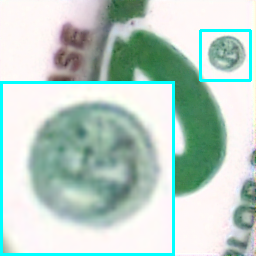
CBDNet [24]

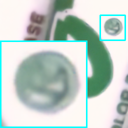
RIDNet [5]

VDN [50]

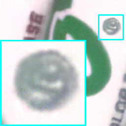
DANet [51]

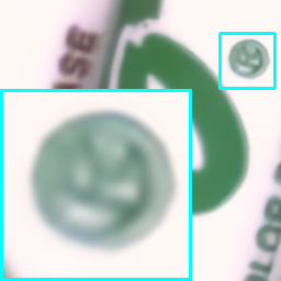
InvDN (Ours)

Figure 1: A real noisy image from the SIDD [2] dataset. Compared with RIDNet [5] and DANet [51], InvDN does not over-smooth. In addition, in comparison with all the other methods, InvDN restores more crisp edges and produces fewer artifacts. The examples are best viewed in color on a high-resolution display with zooming in.

Image denoising aims to restore clean images from noisy observations. Traditional approaches model denoising as a maximum a posteriori (MAP) optimization problem, with assumptions on the distribution of noise [38, 57, 12], and natural image priors [16, 39, 47]. Although these algorithms achieve satisfactory performance on removing synthetic noise, their effectiveness on real-world noise is compromised since their assumptions deviate from those in real-world scenarios. Recently, convolutional neural networks (CNNs) have achieved superior denoising performance [53, 54]. These CNNs learn the features of images from a large number of clean and noisy image pairs. However, since real noise is very complex, to achieve better denoising accuracy, CNN denoising models have become increasingly large and complicated [50, 51, 52]. Thus, although some methods can achieve very impressive denoising results, they may not be practical in realistic scenarios such as deploying the model on edge equipment like smartphones and motion sensing devices.

Currently, a substantial amount of research has been devoted to developing neural networks that are invertible [18, 41, 25, 9]. For image denoising, invertible networks are advantageous from the following three aspects: (1) the model is light, as encoding and decoding use the same parameters; (2) they preserve details of the input data since invertible networks are information-lossless [36]; (3) they save memory during back-propagation because they use a constant amount of memory to compute gradients, regardless of the depth of the network [23]. Hence, invertible models are suitable for small devices like smartphones. We thus study employing invertible networks to address the problem of image denoising. However, applying such networks to remove noise is non-trivial. The original inputs and the reversed results of the traditional invertible models follow the same distribution [19, 31, 46]. In contrast, for image denoising, the input is noisy, and the restored image is clean, following two different distributions. Therefore, invertible denoising networks are required to abandon the noise in the latent space before the reversion. Due to this difficulty, noise removal has not previously been studied and deployed in invertible literature and models.

In this paper, we propose an invertible denoising network, InvDN, to resolve the above difficulties. Unlike previous invertible models, two different latent variables are involved; one incorporates noise and high-frequency clean contents while the other only encodes the clean part. During the forward pass, InvDN transforms the input image to a downscaled latent representation with an increased number of channels. We train InvDN to make the first three channels of the latent representation the same as the low-resolution clean image. Since invertible networks preserve all the information of the input [36], noisy signals are in the rest of the channels. To remove noise completely, we discard all the channels that contain noise. However, as a side-effect, we also lose some information corresponding to the high-resolution clean image. To reconstruct such missing information, we sample a new latent variable from a prior distribution and combine it with the low-resolution image to restore the clean image.

Our contributions are as follows:

• We are the first to design invertible networks for real image denoising to the best of our knowledge.

• The latent variable of traditional invertible networks follows a single distribution. Instead, InvDN has two latent variables following two different distributions. Thus, InvDN can not only restore clean images but also generate new noisy images.

• We achieve a new state-of-the-art (SOTA) result on the SIDD test set, using far fewer parameters and less run time than the previous SOTA methods.

• InvDN is able to generate new noisy images that are more similar to the original noisy ones.

2 Related Work

In this section, we summarize and discuss the development and recent trends in image denoising. The widely used denoising methods can be classified into traditional methods and current data-driven deep learning methods.

Traditional Methods. Model-driven denoising methods usually construct a MAP optimization problem with a loss and a regularization term. The assumptions on the noise distribution are needed for most traditional methods to build the model. One assumed distribution is the Mixture of Gaussian, which is used as an approximator for noise on natural patches or patch groups [58, 13, 49]. The regularization term is usually based on the clean image’s prior. Total variation [43] denoising uses the statistical characteristics of images to remove noise. Sparsity [37] is enforced in dictionary learning methods [20], to learn over-complete dictionaries from clean images. Non-local similarity [11, 21] methods employ non-local patches that share similar patterns. Such a strategy is adopted by the notable BM3D [17] and NLM [11]. However, these models are limited due to the assumptions on the prior of spatially invariant noise or clean images, which are often different from real cases, where the noise is spatially variant.

Data-driven Deep Learning Denoising. Recent years have seen rapid progress in the deep learning methods, boosting the denoising performance to a large extent. The early deep models focus on synthetic noisy image denoising due to a lack of real data. As some large real noise datasets, such as DND [40] and SIDD [2], have been presented, current research focuses on blind real image denoising. There are two main streams in real image denoising. One is to adapt the methods that work well on the synthetic datasets to the real datasets while considering the gap between these two domains [54, 24]. The current most competitive method along this direction is AINDNet [29], which applies transfer learning from synthetic to real denoising with the Adaptive Instance Normalization operations.

The other direction is to model real noise with more complicated distributions and design new network architectures [10, 14]. VDN [50] proposed by Yue et al.assumes that noise follows an inverse Gamma distribution, and the clean image we observe is a conjugate Gaussian prior of the unavailable real clean images. They propose a new training objective based on these assumptions and use two parallel branches to learn these two distributions in the same network. Its potential limitation is that the assumptions are not suitable when the noise distribution becomes complicated. Later, DANet [51] abandons the assumptions for noise distributions and employs a GAN framework to train the model. Two parallel branches are also employed in this architecture: one for denoising and the other for noise generation. This design concept is that the three kinds of image pairs (clean and noisy, clean and generated noisy, as well as denoised and noisy) follow the same distribution, so they use a discriminator to train the model. The potential limitation is that GAN-based models’ training is unstable and thus takes longer to converge [8]. Furthermore, both VDN and DANet employ Unet [42] in the parallel branches, making their models very large.

To compress the model size, we explore invertible networks. To the best of our knowledge, few studies apply invertible networks in denoising literature. Noise Flow [1] introduces an invertible architecture to learn real noise distributions to generate real noise as a way of data augmentation. Generating noisy images with Noise Flow requires extra information apart from the sRGB images, including raw-RGB images, ISO, and camera-specific values. They do not propose new denoising backbones. So far, no invertible network for real image denoising has been reported.

3 Invertible Denoising Network

In this paper, we present a novel denoising architecture consisting of invertible modules, , Invertible Denoising Network (InvDN). For completeness, in this section, we first provide the background of invertible neural networks and then present the details of InvDN.

3.1 Invertible Neural Network

Invertible networks are originally designed for unsupervised learning of probabilistic models [19]. These networks can transform a distribution to another distribution through a bijective function without losing information [36]. Thus, it can learn the exact density of observations. Using invertible networks, images following a complex distribution can be generated through mapping a given latent variable $\mathbf{z}$, which follows a simple distribution $p_{\mathbf{z}}(\mathbf{z})$, to an image instance $\mathbf{x}\sim p_{\mathbf{x}}(\mathbf{x})$, , $\mathbf{x}=f(\mathbf{z})$, where $f$ is the bijective function learned by the network. Due to the bijective mapping and exact density estimation properties, invertible networks have received increasing attention in recent years and have been applied successfully in applications such as image generation [19, 31] and rescaling [46].

3.2 Challenges in Denoising with Invertible Models

Applying invertible models in denoising is different from other applications. The widely used invertible networks employed in image generation [19, 31] and rescaling [46] consider the input and the reverted image to follow the same distribution. Such applications are straightforward candidates for invertible models. Image denoising, however, takes a noisy image as input and reconstructs a clean one, , the input and the reverted outcome follow two different distributions. On the other hand, an invertible transform does not lose any information during the transformation. However, the lossless property of invertibility is not desired for image denoising since the noise information remains while we transform an input image into latent variables. If we can disentangle the noisy and clean signals during an invertible transformation, we may reconstruct a clean image without worrying about losing any important information by abandoning the noisy information. In the following section, we present one way to obtain a clean signal through an invertible transformation.

3.3 Concept of Design

We denote the original noisy image as $\mathbf{y}$, its clean version as $\mathbf{x}$ and the noise as $\mathbf{n}$. We have: $p(\mathbf{y})=p(\mathbf{x},\mathbf{n})=p(\mathbf{x})p(\mathbf{n}|\mathbf{x})$. Using the invertible network, the learned latent representation of observation $\mathbf{y}$ contains both noise and clean information. It should be noted that it is non-trivial to disentangle them and abandon only the noisy part.

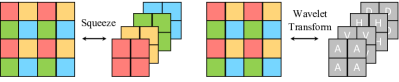
Figure 2: Invertible Transforms. The Squeeze operation on the left extracts features according to a checkerboard pattern. The Wavelet Transformation on the right extracts the average pooling of the image, as well as the vertical, horizontal and diagonal derivatives.

On the other hand, invertible networks utilize different feature extraction approaches comparing with existing deep denoising models. Existing ones usually employ convolutional layers with padding to extract features. However, they are not invertible due to two reasons: Firstly, the padding makes the network non-invertible; secondly, the parameter matrices of convolutions may not be full-rank. Thus, to ensure invertibility, rather than using convolutional layers, it is necessary to utilize invertible feature extraction methods, such as the Squeeze layer [31] and Haar Wavelet Transformation [7], as presented in Fig. 2. The Squeeze operation reshapes the input into feature maps with more channels according to a checkerboard pattern. Haar Wavelet Transformation extracts the average pooling of the original input as well as the vertical, horizontal, and diagonal derivatives. As a result, the spatial size of the feature maps extracted by the invertible methods is inevitably downscaled.

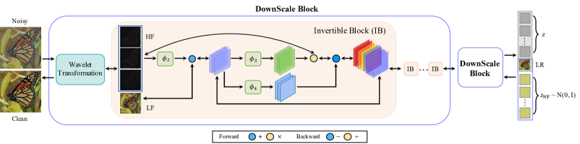
Figure 3: Invertible Denoising Network. InvDN consists of several DownScale Blocks. Each DownScale Block has a Wavelet Transformation layer to reduce the spatial resolution by 2$\times$ and increase the number of channels by 4$\times$, followed by several Invertible Blocks. In the forward pass, we learn the low-resolution image and a latent variable $\mathbf{z}$ from the noisy input. In the backward procedure, we randomly sample $\mathbf{z}_{\text{HF}}$ from $\mathcal{N}(\mathbf{0},\mathbf{I})$ and combine it with LR to restore the clean image.

Therefore, instead of disentangling the clean and noisy signals directly, we aim to separate the low-resolution and high-frequency components of a noisy image. The sampling theory [22] indicates that during the downsampling process, the high-frequency signals are discarded. Since invertible networks are information-lossless [36], if we make the first three channels of the transformed latent representation to be the same as the downsampled clean image, high-frequency information will be encoded in the remaining channels. Based on the observation that the high-frequency information contains noise as well, we abandon all high-frequency representations before inversion to reconstruct a clean image from low-resolution components. We formally describe the process as follows:

$$p(\mathbf{y})=p(\mathbf{x}_{\text{LR}},\mathbf{x}_{\text{HF}},\mathbf{n})=p(\mathbf{x}_{\text{LR}})p(\mathbf{x}_{\text{HF}},\mathbf{n}|\mathbf{x}_{\text{LR}}),$$

where $\mathbf{x}_{\text{LR}}$ represents the low-resolution clean image. We use $\mathbf{x}_{\text{HF}}$ to represent the high-frequency contents that cannot be obtained by $\mathbf{x}_{\text{LR}}$ when reconstructing the original clean image. Since it is challenging to disentangle $\mathbf{x}_{\text{HF}}$ and $\mathbf{n}$, we abandon all the channels representing $\mathbf{z}\sim p(\mathbf{x}_{\text{HF}},\mathbf{n}|\mathbf{x}_{\text{LR}})$ to remove spatially variant noise completely. Nevertheless, a side-effect is the loss of $\mathbf{x}_{\text{HF}}$. To reconstruct $\mathbf{x}_{\text{HF}}$, we sample $\mathbf{z}_{\text{HF}}\sim\mathcal{N}(\mathbf{0},\mathbf{I})$ and train our invertible network to transform $\mathbf{z}_{\text{HF}}$, in conjunction with $\mathbf{x}_{\text{LR}}$, to restore the clean image $\mathbf{x}$. In this way, the lost high-frequency clean details $\mathbf{x}_{\text{HF}}$ is embedded in the latent variable $\mathbf{z}_{\text{HF}}$.

3.4 Network Architecture

We first employ a supervised approach to guide the network to separate high-frequency and low-resolution components during transformation. After some invertible transformation $g$, the noisy image $\mathbf{y}$ is transformed into its corresponding low-resolution clean image and high-frequency encoding $\mathbf{z}$, $g(\mathbf{y})=[g(\mathbf{y})_{\text{LR}};\mathbf{z}]$. We minimize the following forward objective

$$\mathcal{L}_{\text{forw}}(\mathbf{y},\mathbf{x}_{\text{LR}}) =\frac{1}{M}\sum_{i=1}^{M}\left\lVert g(\mathbf{y})_{\text{LR}}-\mathbf{x}_{\text{LR}}\right\rVert_{m},$$ (1)

where $g(\mathbf{y})_{\text{LR}}$ is the low-frequency components learned by the network, corresponding to three channels of the output representation in the forward pass. $M$ is the number of pixels. $||\cdot||_{m}$ is the $m$-norm and $m$ can be either 1 or 2. To obtain the ground truth low-resolution image $\mathbf{x}_{\text{LR}}$, we down-sample the clean image $\mathbf{x}$ via bicubic transformation.

To restore the clean image with $g(\mathbf{y})_{\text{LR}}$, we use inverse transform $g^{-1}([g(\mathbf{y})_{\text{LR}};\mathbf{z}_{\text{HF}}])$ with random variable $\mathbf{z}_{\text{HF}}$ sampled from normal distribution $\mathcal{N}(\mathbf{0},\mathbf{I})$. The backward objective is written as

$$\mathcal{L}_{\text{back}}(g(\mathbf{y})_{\text{LR}},\mathbf{x}) =\frac{1}{N}\sum_{i=1}^{N}\left\lVert g^{-1}([g(\mathbf{y})_{\text{LR}};\mathbf{z}_{\text{HF}}])-\mathbf{x}\right\rVert_{m},$$

where $\mathbf{x}$ is the clean image. $N$ is the number of pixels. We train the invertible transformation $g$ by simultaneously utilizing both forward and backward objectives.

Inspired by [46, 7, 19], the invertible transform $g$ we present is of a multi-scale architecture, consisting of several down-scale blocks. Each down-scale block consists of an invertible wavelet transformation followed by a series of invertible blocks. The overall architecture of the InvDN model is demonstrated in Fig. 3.

Table 1: The invertible block operations in the down-scale block. In the forward pass, the input and output to each block are denoted as $\mathbf{u}^{i}$ and $\mathbf{u}^{i+1}$. During the backward pass, only Plus ($+$) and Multiply ($\odot$) needs to be inverted. $\operatorname{\phi}_{1}$, $\operatorname{\phi}_{2}$, $\operatorname{\phi}_{3}$ and $\operatorname{\phi}_{4}$ do not need to be inverted. Thus, they can be any neural networks.

#	Forward Operation	Backward Operation	Specification
R1	$\mathbf{u}^{i}_{a}$, $\mathbf{u}^{i}_{b}=\operatorname{Split}(\mathbf{u}^{i})$	$\mathbf{u}^{i+1}_{a}$, $\mathbf{u}^{i+1}_{b}=\operatorname{Split}(\mathbf{u}^{i+1})$	$\operatorname{Split}(\cdot)$ is splitting channel-wise.
R2	$\mathbf{u}^{i+1}_{a}=\mathbf{u}^{i}_{a}\odot\operatorname{exp}(\operatorname{\phi}_{1}(\mathbf{u}^{i}_{b}))+\operatorname{\phi}_{2}(\mathbf{u}^{i}_{b})$	$\mathbf{u}^{i}_{b}=(\mathbf{u}^{i+1}_{b}-\operatorname{\phi}_{4}(\mathbf{u}^{i+1}_{a}))/\operatorname{exp}(\operatorname{\phi}_{3}(\mathbf{u}^{i+1}_{a})$)	$\operatorname{\phi}_{1}$, $\operatorname{\phi}_{2}$, $\operatorname{\phi}_{3}$ and $\operatorname{\phi}_{4}$ can be any neural networks. $\odot$ is the multiply operation.
R3	$\mathbf{u}^{i+1}_{b}=\mathbf{u}^{i}_{b}\odot\operatorname{exp}(\operatorname{\phi}_{3}(\mathbf{u}^{i+1}_{a}))+\operatorname{\phi}_{4}(\mathbf{u}^{i+1}_{a})$	$\mathbf{u}^{i}_{a}=(\mathbf{u}^{i+1}_{a}-\operatorname{\phi}_{2}(\mathbf{u}^{i}_{b}))/\operatorname{exp}(\operatorname{\phi}_{1}(\mathbf{u}^{i}_{b})$)
R4	$\mathbf{u}^{i+1}=\operatorname{Concat}(\mathbf{u}^{i+1}_{a},\mathbf{u}^{i+1}_{b})$	$\mathbf{u}^{i}=\operatorname{Concat}(\mathbf{u}^{i}_{a}$, $\mathbf{u}^{i}_{b})$	$\operatorname{Concat}(\cdot)$ is concating channel-wise.

Invertible Wavelet Transformation. Since we aim to learn the low-resolution clean image in the forward pass, we apply invertible discrete wavelet transformations (DWTs), specifically Haar wavelet transformation, to increase feature channels and to down-sample feature maps. After the wavelet transformation, the input image or an intermediate feature map with the size of $(H,W,C)$ is transformed into a new feature map of size $(H/2,W/2,4C)$. Haar wavelets decompose an input image into one low-frequency representation and three high-frequency representations in the vertical, horizontal, and diagonal direction [32]. Other DWTs can also be exploited, such as Haar, Daubechies, and Coiflet wavelets [46, 7].

Invertible Block. The wavelet transformation layer in each down-scale block splits the representation into low- and high-frequency signals, which are further processed by a series of invertible blocks. The invertible block we follow in this work is the coupling layer [19]. Suppose the block’s input is $\mathbf{u}^{i}$, and output is $\mathbf{u}^{i+1}$. This block’s operations in the forward and backward pass are listed in Subsec. 3.4.

$\operatorname{Split}(\cdot)$ operation divides input feature map $\mathbf{u}^{i}$, which has the size of $(H/2,W/2,4C)$, into $\mathbf{u}_{a}^{i}$ and $\mathbf{u}_{b}^{i}$, corresponding to the low-frequency image representations of size $(H/2,W/2,C)$ and the high-frequency features (such as texture and noise) of size $(H/2,W/2,3C)$, respectively.

In R2 and R3 of Subsec. 3.4, during the backward pass, only the Plus ($+$) and Multiply ($\odot$) operations are inverted to Minus ($-$) and Divide ($/$) while the operations performed by $\operatorname{\phi}_{1}$, $\operatorname{\phi}_{2}$, $\operatorname{\phi}_{3}$ and $\operatorname{\phi}_{4}$ are not required to be invertible. Thus, $\operatorname{\phi}_{1}$, $\operatorname{\phi}_{2}$, $\operatorname{\phi}_{3}$ and $\operatorname{\phi}_{4}$ can be any networks, including convolutional layers with paddings. Since the skip connection is shown to be crucial for deep denoising networks [50, 51], we simplify the forward operation in R2 as

$$\mathbf{u}^{i+1}_{a}=\mathbf{u}^{i}_{a}+\operatorname{\phi}_{2}(\mathbf{u}^{i}_{b}).$$ (2)

The low-frequency features can be passed to deep layers with this approach. We use the residual block as operations $\operatorname{\phi}_{2}$, $\operatorname{\phi}_{3}$ and $\operatorname{\phi}_{4}$.

$\operatorname{Concat}(\cdot)$ is the inverse operation of $\operatorname{Split}(\cdot)$, which concatenates the feature maps along channels and passes them into the next module.

4 Experiment

Noisy

CBDNet [24]

RIDNet [5]

VDN [50]

DANet [51]

InvDN (Ours)

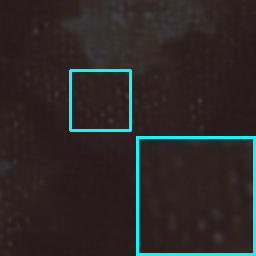
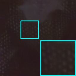
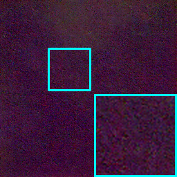
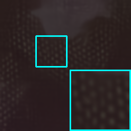
(a) SIDD [2] visualization examples. InvDN produces fewer artifacts and more clear patterns, even in dark environments.

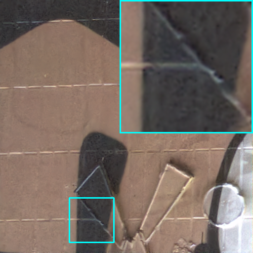
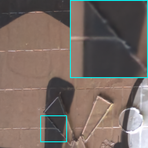
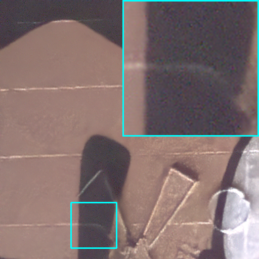
(b) DND [40] visualization examples. InvDN can reconstruct the subtle edges very clearly

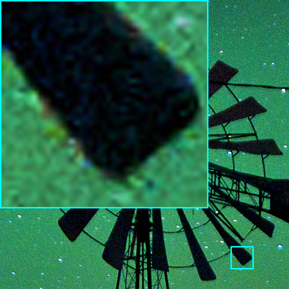
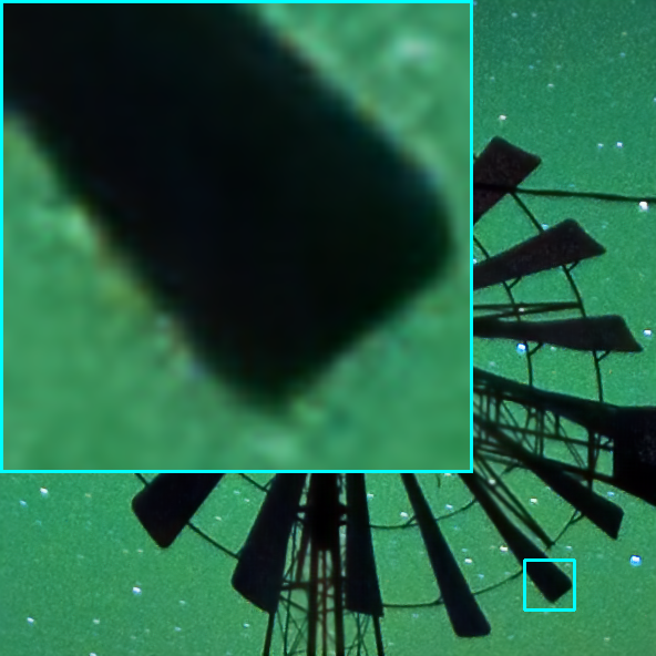
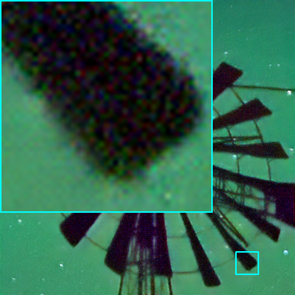
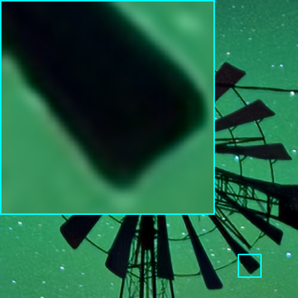
(c) RNI visualization examples. InvDN produces fewer stains and more accurate edges without artifacts.

Figure 4: Visualization results of InvDN compared against other competitive models. Boxed regions are zoomed results. Best viewed in color on a high-resolution display.

In this section, we present some empirical performances of InvDN on real denoising tasks.

4.1 Dataset

We evaluate InvDN on three real-world denoising benchmarks, , SIDD [2], DND [40], and RNI [33].

SIDD [2] is taken by five smartphone cameras with small apertures and sensor sizes. We use the medium version of SIDD as the training set, containing 320 clean-noisy pairs for training and 1280 cropped patches from the other 40 pairs for validation. In each iteration of training, we crop the input image into multiple $144\times 144$ patches to feed into the network. The reported test results are obtained via an online submission system.

DND [40] is captured by four consumer-grade cameras of differing sensor sizes. It contains 50 pairs of real-world noisy and approximately noise-free images. These images are cropped into 1000 patches of size $512\times 512$. Similarly to SIDD, the performance is evaluated by submitting the outputs of the methods to the online system.

RNI15 [33] is composed of 15 real-world noisy images without ground-truths. Therefore, we only provide visual comparisons on this dataset.

4.2 Training Details.

Our InvDN has two down-scale blocks, each of which is composed of eight invertible blocks. All the models are trained with Adam [30] as the optimizer, with momentum of $\beta_{1}=0.9,\beta_{2}=0.999$. The batch size is set as 14, and the initial learning rate is fixed at $2\times 10^{-4}$, which decays by half every 50k iterations. PyTorch is used as the implementation framework, and training is performed on a single 2080-Ti GPU. We augment the data with horizontal and vertical flipping, as well as random rotations of $90\times\theta$ where $\theta=0,1,2,3$.

4.3 Experimental Results

We evaluate the methods by commonly used metrics such as Peak Signal-to-Noise Ratio (PSNR) and Structural Similarity Index Measure (SSIM), which are also available on the real-noisy DND and SIDD websites.

Quantitative Measure. As mentioned before, we train InvDN using the SIDD medium training set. DND does not provide the training set; therefore, we use the model trained on SIDD. For a fair comparison, the PSNR of other competitive models on the test set is directly taken from the official DND and SIDD leaderboards and verified from the respective articles. Table 2 reports the test results of different denoising models. We can observe that the number of model parameters is directly positively correlated to the model’s performance. From RIDNet [5] to DANet [51], the number of model parameters increases from 1.49 million (M) to 63.01M with a slight improvement in PSNR.

Nevertheless, InvDN reverses the trend, having only 2.64M parameters. Compared with the most recently proposed SOTA DANet, InvDN only uses less than 4.2% of the number of parameters of DANet. Although InvDN has far fewer parameters, the denoising performance on the test set is better than all the recently proposed denoising models, achieving a new SOTA result for the SIDD dataset. The performance of InvDN is also comparable with that of the recent competitive models on DND, indicating the generalization ability of our lightweight denoising model.

Qualitative Measure. To further illustrate the better performance of InvDN against other methods, in Fig. 4, we show denoised visual results on images from three different datasets, SIDD, DND and RNI15. The first row of the figure illustrates that InvDN restores well-shaped patterns, while other competing techniques induce blurry textures and artifacts. Furthermore, the second row depicts that InvDN recovers the subtle edges very clearly, whereas other models bring artifacts and over-smoothness. Finally, from the third row, we observe that InvDN reconstructs accurate edges compared to other models that introduce blockiness, fuzziness, and random dots, particularly along the edges.

Table 2: Comparison of InvDN against other competitive algorithms. All the results are obtained without MC-ensemble for fair comparison. “Infer time” presents the inference time of one $256\times 256$ image in gigaFLOPs. A tick represents containing the corresponding functionality. The best results are emphasized with red.

							DND		SIDD
Method	Blind Denoising	MultiScale	Noise Generation	Invertible	Num of Parameters	Infer Time	PSNR	SSIM	PSNR	SSIM
DnCNN [53]	✓				0.56	–	32.43	0.7900	23.66	0.583
EPLL [59]					–	–	33.51	0.8244	27.11	0.870
TNRD [15]					–	–	33.65	0.8306	24.73	0.643
FFDNet [54]					0.48	–	34.40	0.8474	–	–
BM3D [17]					–	–	34.51	0.8507	25.65	0.685
NI [3]	✓				–	–	35.11	0.8778	–	–
NC [34]	✓				–	–	35.43	0.8841	–	–
KSVD [4]					–	–	36.49	0.8978	26.88	0.842
TWSC [48]					–	–	37.96	0.9416	–	–
CBDNet [24]	✓		✓		4.34	80.76	38.06	0.9421	33.28	0.868
IERD [6]					–	–	39.20	0.9524	–	–
RIDNet [5]	✓				1.49	196.52	39.26	0.9528	–	–
PRIDNet [56]	✓	✓			–	–	39.42	0.9528	–	–
DRDN [44]	✓				–	–	39.43	0.9531	–	–
GradNet [35]	✓				1.60	–	39.44	0.9543	38.34	0.946
AINDNet [29]	✓				13.76	–	39.53	0.9561	39.08	0.953
DPDN [26]	✓				–	–	39.83	0.9537	–	–
MIRNet [52]	✓	✓			31.78	1569.88	39.88	0.9563	–	–
VDN [50]	✓				7.81	99.00	39.38	0.9518	39.26	0.955
DANet [51]	✓		✓		63.01	65.62	39.58	0.9545	39.25	0.955
Ours	✓	✓	✓	✓	2.64	47.80	39.57	0.9522	39.28	0.955

4.4 Ablation Study

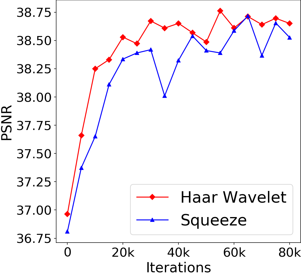
(a) Transformation

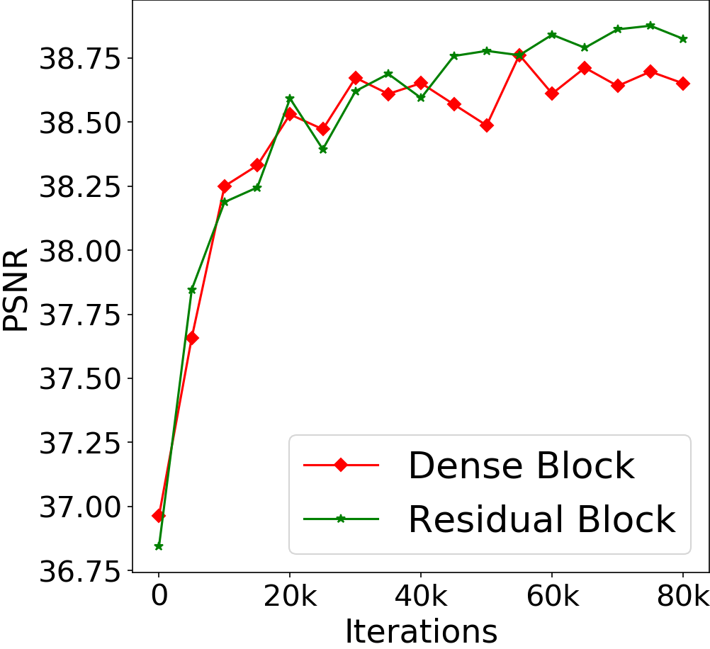
(b) $\operatorname{\phi}_{i}$

Figure 5: Comparisons on training with different network components. (a) illustrates the difference between using Haar wavelet and squeeze as the transformation layer. (b) shows training curves employing residual block and dense block as $\operatorname{\phi}_{2}$, $\operatorname{\phi}_{3}$ and $\operatorname{\phi}_{4}$ separately.

Squeeze vs Wavelet Transform. We compare the difference of employing the squeeze [31] and Haar wavelet transform in down-scale blocks. We report PSNR on the validation set of the same iteration during training in 4(a). The remaining network components and the parameter settings are the same. We observe that using Haar wavelet converges faster and is more stable than the squeeze operation.

Table 3: Comparisons on the denoising accuracy of different numbers of down-scale blocks and invertible blocks.

Scale	DownScale Blocks	Invertible Blocks	PSNR
X2	1	8	38.00
X4	2	8	38.40
X8	3	8	37.69
X2	1	16	38.30
X4	2	16	38.61
X8	3	16	38.15

Residual Block vs. Dense Block. Next, we provide comparison between different blocks ($\operatorname{\phi_{i}}$) in our network in 4(b). The architecture with residual block achieves higher denoising accuracy than dense block used by [46]. Moreover, the network with residual block has far fewer parameters (2.6M) than that using the dense block (4.3M).

Table 4: Comparisons on different combinations of losses on the SIDD validation set.

Losses	Forw	Back	Forw	Back	Forw	Back	Forw	Back	Forw	Back	Forw	Back	Forw	Back
L1	✓	✓	✓			✓				✓		✓		✓
L2				✓	✓		✓	✓	✓		✓		✓
Gradient Loss										✓				✓
SSIM Loss												✓		✓
PSNR	38.67		38.29		38.88		38.73		38.74		38.80		38.78

Number of Down-Scale and Invertible Blocks. Now, we study the denoising performance of InvDN with different numbers of down-scale and invertible blocks. We report the PSNR results on the validation set from the same iteration. We discover that increasing the number of invertible blocks boosts denoising accuracy consistently, regardless of the number of down-scale blocks. Moreover, when fixing the number of invertible blocks, we observe that using two down-scale blocks leads to the best denoising effect.

Investigation of Loss Functions. InvDN requires applying loss functions during training for both the low and high-resolution images to minimize the difference between denoised and clean images. As described in Subsec. 3.4, both $\ell_{1}$- and $\ell_{2}$- norms are applicable. We investigate InvDN’s performance via different combinations of loss functions for producing low and high-resolution images. We compare the PSNR results on the SIDD validation set at the same iteration and report the results in Table 4. We observe that employing $\ell_{2}$ for low-resolution images and $\ell_{1}$ for high-resolution images achieves the highest performance. Apart from $\ell_{1}$ and $\ell_{2}$, we also explore other loss function candidates to further improve the denoising effects. We apply the gradient loss [35] and the SSIM loss [55] to minimize the difference between two images from the perspectives of image derivative and structures. However, neither the gradient nor the SSIM loss improves the denoising performance.

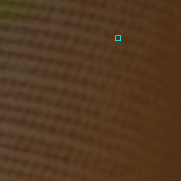
(a) Ground- Truth

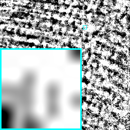
(b) Before MC Self-Ensemble

(c) After MC Self-Ensemble

Figure 6: Visualization of denoising performance before and after MC self-ensemble. (b) and (c) reflect the difference between the denoised image and the ground-truth. Darker means more difference, indicating poorer denoising.

Table 5: AKLD of generated noisy images by different models. Lower is better. The lowest AKLD is in red.

CBDNet	ULRD	GRDN	Noise Flow	DANet	InvDN
[24]	[10]	[28]	[1]	[51]	(Ours)
0.728	0.545	0.443	0.312	0.212	0.059

4.5 Monte Carlo Self Ensemble

To further improve InvDN’s denoising effect without using extra data and training, we introduce Monte Carlo (MC) self-ensemble. We sample the latent variable $\mathbf{z}_{\text{HF}}$ multiple times, resulting in a set of latent variables $\{\mathbf{z}_{\text{HF}}^{i}\}_{i=1}^{N}$, where for each $\mathbf{z}_{\text{HF}}^{i}$, a corresponding denoised image $\hat{x}_{i}$ is obtained. The final output is the average of $\{\hat{x}_{i}\}_{i=1}^{N}$. By the law of large numbers [45], the averaged image is closer to the ground-truth than any individual $\hat{x}_{i}$. In Fig. 6, we visualize the denoising results before and after using MC self-ensembling by setting the MC size to 16. The contrast between the residual images before and after MC self-ensemble indicates that it further reduces the noise in the denoised image. Quantitatively, 83.35% images witness a performance boost on the SIDD validation set.

4.6 Analysis of Distributions of $\mathbf{z}$

For InvDN, there are two types of latent variables: one corresponds to the original high-frequency signal $\mathbf{z}$ containing noise, and the other sampled $\mathbf{z}_{\text{HF}}$ from $\mathcal{N}(\mathbf{0},\mathbf{I})$ representing clean details. To analyze, we obtain 500 pairs of $\mathbf{z}$ and $\mathbf{z}_{\text{HF}}$ from the SIDD validation set. We vectorize each latent variable and plot them in a 3D space with PCA [27]. As 6(a) shows, $\mathbf{z}$ and $\mathbf{z}_{\text{HF}}$ follow two different distributions.

For the sake of fair comparison, we only train InvDN on the benchmark SIDD training set. However, InvDN also supports generating more noisy images for data augmentation. To generate augmented data, we first conduct sampling $\mathbf{z}$. We introduce a tiny disturbance to $\mathbf{z}$ as $\mathbf{z}^{\prime}=\mathbf{z}+\epsilon\cdot\mathbf{v}$, where $\mathbf{v}\sim\mathcal{N}(\mathbf{0},\mathbf{I})$ and $\epsilon$ is set as $2\times 10^{-4}$. We expect the reverted image of $\mathbf{z}^{\prime}$ to have the same background clean image, yet with a different noise. We visualize the reverted images of $\mathbf{z}$ and $\mathbf{z}^{\prime}$ in 6(b) and 6(c), exhibiting visually different noise corresponding to $\mathbf{z}$ and $\mathbf{z}^{\prime}$.

To quantitatively evaluate the quality of our generated noisy images, we follow the average KL divergence (AKLD) metric introduced by DANet [51] to measure the similarity between the original and the generated noise, as shown in Table 5. It should be noted here that Noise Flow [1] requires raw-RGB images, ISO, and CAM information to generate noisy images; in other words, it needs the training images as inputs. The AKLD results in Table 5 demonstrate that our generated noisy images are closer to the original noisy images by a large margin.

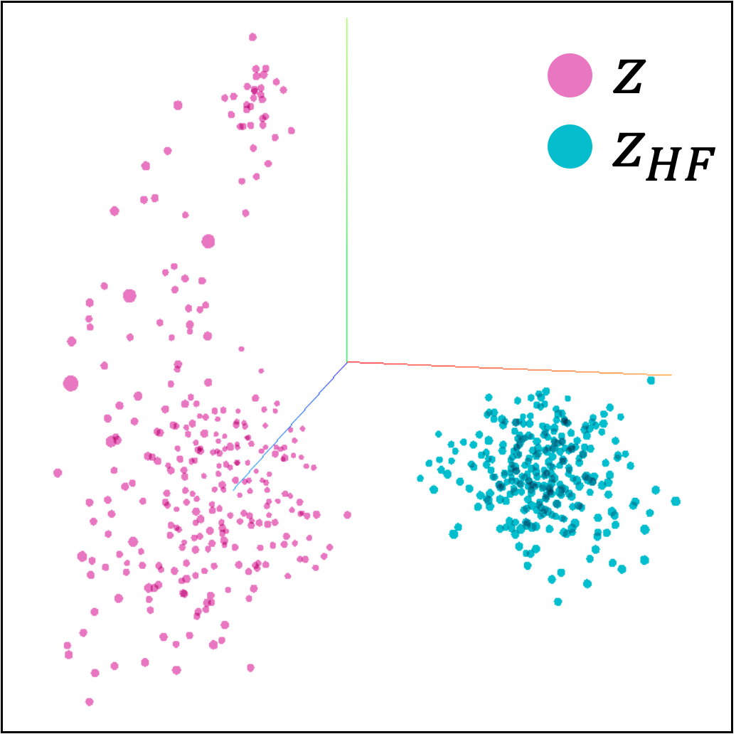
(a) Distributions

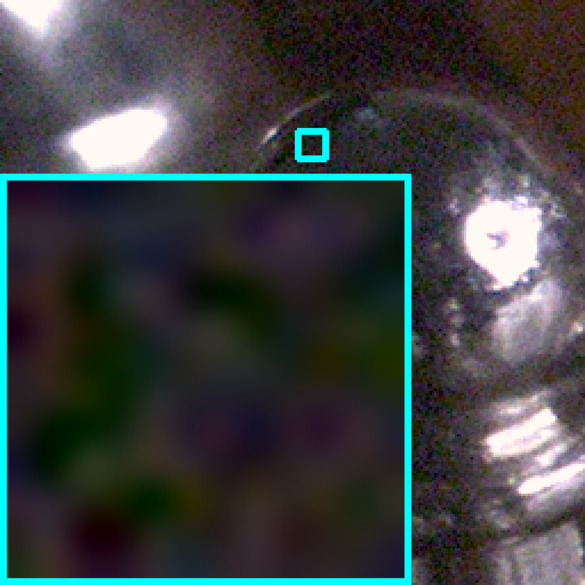
(b) Original

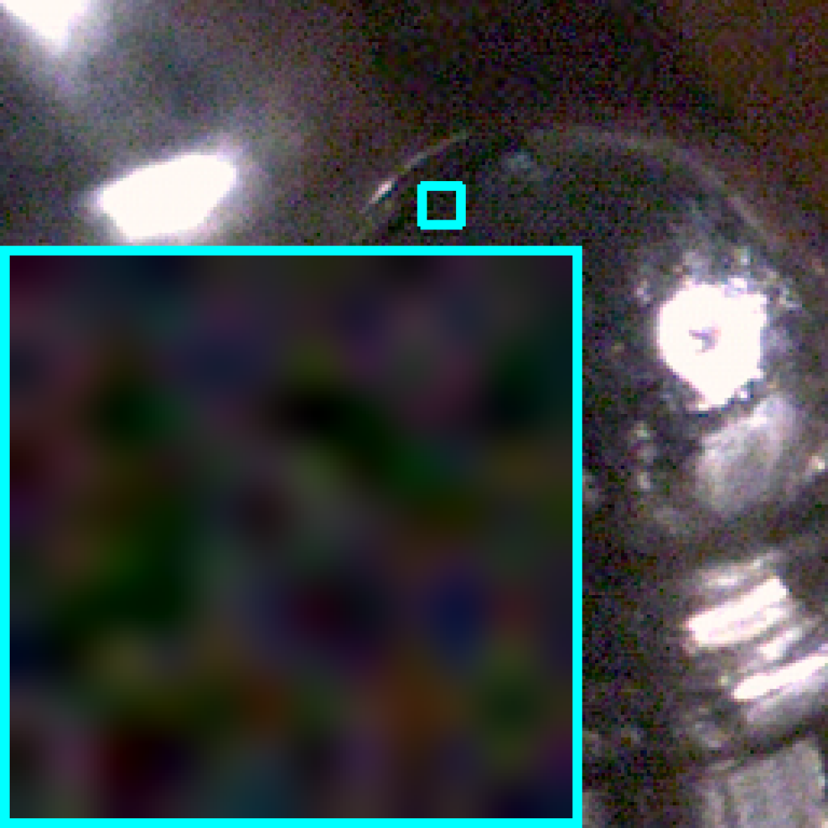
(c) Generated

Figure 7: (a) PCA visualization results of the two distributions corresponding to the noisy latent representations $\mathbf{z}$ (pink) and the clean samples $\mathbf{z}_{\text{HF}}$ (blue). (b) Original noisy image from the SIDD validation set. (c) The generated noisy image by InvDN corresponding to (b).

5 Conclusion

This paper is the first to study real image denoising with invertible networks. In previous invertible models, the input and the reversed output follow the same distribution. However, for image denoising, the input is noisy, and the restored outcome is clean, following two different distributions. To address this issue, our proposed InvDN transforms the noisy input into a low-resolution clean image as well as a latent representation containing noise. As a result, InvDN can both remove and generate noise. For noise removal, we replace the noisy representation with a new one sampled from a prior distribution to restore clean images; for noise generation, we alter the noisy latent vector to reconstruct new noisy images. Extensive experiments on three real-noise datasets demonstrate the effectiveness of our proposed model in both removing and generating noise.

Acknowledgments: This work was partly supported by Institute of Information & communications Technology Planning & Evaluation (IITP) grant funded by the Korea government(MSIT) (No.2019-0-01906, Artificial Intelligence Graduate School Program(POSTECH)).

References

- [1] A. Abdelhamed, M. Brubaker, and M. Brown. Noise flow: Noise modeling with conditional normalizing flows. In 2019 IEEE/CVF International Conference on Computer Vision (ICCV), pages 3165–3173, 2019.
- [2] Abdelrahman Abdelhamed, Stephen Lin, and Michael S. Brown. A high-quality denoising dataset for smartphone cameras. In IEEE Conference on Computer Vision and Pattern Recognition (CVPR), June 2018.
- [3] ABSoft. Neat image.
- [4] M. Aharon, M. Elad, and A. Bruckstein. K-svd: An algorithm for designing overcomplete dictionaries for sparse representation. IEEE Transactions on Signal Processing, 54(11):4311–4322, Nov 2006.
- [5] Saeed Anwar and Nick Barnes. Real image denoising with feature attention. In Proceedings of the IEEE International Conference on Computer Vision, pages 3155–3164, 2019.
- [6] Saeed Anwar, Cong Phuoc Huynh, and Fatih Porikli. Identity enhanced residual image denoising. In Proceedings of the IEEE/CVF Conference on Computer Vision and Pattern Recognition Workshops, pages 520–521, 2020.
- [7] Lynton Ardizzone, Carsten Lüth, Jakob Kruse, Carsten Rother, and Ullrich Köthe. Guided image generation with conditional invertible neural networks, 2019.
- [8] Martin Arjovsky, Soumith Chintala, and Léon Bottou. Wasserstein generative adversarial networks. In Proceedings of the 34th International Conference on Machine Learning-Volume 70, pages 214–223, 2017.
- [9] Jens Behrmann, Will Grathwohl, Ricky T. Q. Chen, David Duvenaud, and Joern-Henrik Jacobsen. Invertible residual networks. In Kamalika Chaudhuri and Ruslan Salakhutdinov, editors, Proceedings of the 36th International Conference on Machine Learning, volume 97 of Proceedings of Machine Learning Research, pages 573–582. PMLR, 09–15 Jun 2019.
- [10] Tim Brooks, Ben Mildenhall, Tianfan Xue, Jiawen Chen, Dillon Sharlet, and Jonathan T. Barron. Unprocessing images for learned raw denoising. In Proceedings of the IEEE/CVF Conference on Computer Vision and Pattern Recognition (CVPR), June 2019.
- [11] A. Buades, B. Coll, and J. . Morel. A non-local algorithm for image denoising. In 2005 IEEE Computer Society Conference on Computer Vision and Pattern Recognition (CVPR’05), volume 2, pages 60–65 vol. 2, 2005.
- [12] X. Cao, Y. Chen, Q. Zhao, D. Meng, Y. Wang, D. Wang, and Z. Xu. Low-rank matrix factorization under general mixture noise distributions. In 2015 IEEE International Conference on Computer Vision (ICCV), pages 1493–1501, 2015.
- [13] F. Chen, L. Zhang, and H. Yu. External patch prior guided internal clustering for image denoising. In 2015 IEEE International Conference on Computer Vision (ICCV), pages 603–611, 2015.
- [14] Jingwen Chen, Jiawei Chen, Hongyang Chao, and Ming Yang. Image blind denoising with generative adversarial network based noise modeling. In CVPR, June 2018.
- [15] Yunjin Chen and Thomas Pock. Trainable nonlinear reaction diffusion: A flexible framework for fast and effective image restoration. TPAMI, 2017.
- [16] K. Dabov, A. Foi, V. Katkovnik, and K. Egiazarian. Image denoising by sparse 3-d transform-domain collaborative filtering. IEEE Transactions on Image Processing, 16(8):2080–2095, 2007.
- [17] K. Dabov, A. Foi, V. Katkovnik, and K. Egiazarian. Image denoising by sparse 3-d transform-domain collaborative filtering. TIP, 16(8):2080–2095, Aug 2007.
- [18] Laurent Dinh, David Krueger, and Yoshua Bengio. Nice: Non-linear independent components estimation. ICML Workshop, 2014.
- [19] Laurent Dinh, Jascha Sohl-Dickstein, and Samy Bengio. Density estimation using real nvp, 2017.
- [20] W. Dong, X. Li, L. Zhang, and G. Shi. Sparsity-based image denoising via dictionary learning and structural clustering. In CVPR 2011, pages 457–464, 2011.
- [21] A. Foi, V. Katkovnik, and K. Egiazarian. Pointwise shape-adaptive dct for high-quality denoising and deblocking of grayscale and color images. IEEE Transactions on Image Processing, 16(5):1395–1411, 2007.
- [22] Eduardo SL Gastal and Manuel M Oliveira. Spectral remapping for image downscaling. ACM Transactions on Graphics (TOG), 36(4):1–16, 2017.
- [23] Aidan N Gomez, Mengye Ren, Raquel Urtasun, and Roger B Grosse. The reversible residual network: Backpropagation without storing activations. In Advances in neural information processing systems, pages 2214–2224, 2017.
- [24] Shi Guo, Zifei Yan, Kai Zhang, Wangmeng Zuo, and Lei Zhang. Toward convolutional blind denoising of real photographs. CVPR, 2019.
- [25] Jörn-Henrik Jacobsen, Arnold W.M. Smeulders, and Edouard Oyallon. i-revnet: Deep invertible networks. In International Conference on Learning Representations, 2018.
- [26] Yeong Jang, Yoonsik Kim, and Nam Cho. Dual path denoising network for real photographic noise. IEEE Signal Processing Letters, PP:1–1, 05 2020.
- [27] Ian Jolliffe and Jorge Cadima. Principal component analysis: A review and recent developments. Philosophical Transactions of the Royal Society A: Mathematical, Physical and Engineering Sciences, 374:20150202, 04 2016.
- [28] Dong-Wook Kim, Jae Ryun Chung, and Seung-Won Jung. Grdn:grouped residual dense network for real image denoising and gan-based real-world noise modeling. In Proceedings of the IEEE/CVF Conference on Computer Vision and Pattern Recognition (CVPR) Workshops, June 2019.
- [29] Y. Kim, J. Soh, G. Park, and N. Cho. Transfer learning from synthetic to real-noise denoising with adaptive instance normalization. In 2020 IEEE/CVF Conference on Computer Vision and Pattern Recognition (CVPR), pages 3479–3489, Los Alamitos, CA, USA, jun 2020. IEEE Computer Society.
- [30] Diederik P. Kingma and Jimmy Lei Ba. Adam: A method for stochastic optimization. In ICLR 2015 : International Conference on Learning Representations 2015, 2015.
- [31] Diederik P Kingma and Prafulla Dhariwal. Glow: generative flow with invertible 1 1 convolutions. In Proceedings of the 32nd International Conference on Neural Information Processing Systems, pages 10236–10245, 2018.
- [32] Nick Kingsbury and Julian Magarey. Wavelet Transforms in Image Processing, pages 27–46. Birkhäuser Boston, Boston, MA, 1998.
- [33] Marc Lebrun, Miguel Colom, and Jean-Michel Morel. The Noise Clinic: a Blind Image Denoising Algorithm. Image Processing On Line, 5:1–54, 2015.
- [34] Marc Lebrun, Miguel Colom, and Jean-Michel Morel. The Noise Clinic: a Blind Image Denoising Algorithm. Image Processing On Line, 5:1–54, 2015.
- [35] Yang Liu, Saeed Anwar, Liang Zheng, and Qi Tian. Gradnet image denoising. In Proceedings of the IEEE/CVF Conference on Computer Vision and Pattern Recognition Workshops, pages 508–509, 2020.
- [36] Yang Liu, Zhenyue Qin, Saeed Anwar, Sabrina Caldwell, and Tom Gedeon. Are deep neural architectures losing information? invertibility is indispensable. In International Conference on Neural Information Processing (ICONIP), 2020.
- [37] J. Mairal, F. Bach, J. Ponce, G. Sapiro, and A. Zisserman. Non-local sparse models for image restoration. In 2009 IEEE 12th International Conference on Computer Vision, pages 2272–2279, 2009.
- [38] D. Meng and F. De la Torre. Robust matrix factorization with unknown noise. In 2013 IEEE International Conference on Computer Vision, pages 1337–1344, 2013.
- [39] Y. Peng, A. Ganesh, J. Wright, W. Xu, and Y. Ma. Rasl: Robust alignment by sparse and low-rank decomposition for linearly correlated images. IEEE Transactions on Pattern Analysis and Machine Intelligence, 34(11):2233–2246, 2012.
- [40] Tobias Plotz and Stefan Roth. Benchmarking denoising algorithms with real photographs. In Proceedings of the IEEE Conference on Computer Vision and Pattern Recognition (CVPR), July 2017.
- [41] Danilo Rezende and Shakir Mohamed. Variational inference with normalizing flows. In International Conference on Machine Learning, pages 1530–1538, 2015.
- [42] Olaf Ronneberger, Philipp Fischer, and Thomas Brox. U-net: Convolutional networks for biomedical image segmentation. CoRR, abs/1505.04597, 2015.
- [43] Leonid I. Rudin, Stanley Osher, and Emad Fatemi. Nonlinear total variation based noise removal algorithms. Physica D Nonlinear Phenomena, 60(1-4):259–268, Nov. 1992.
- [44] Yuda Song, Yunfang Zhu, and Xin Du. Dynamic residual dense network for image denoising. Sensors, 19(17):3809, Sep 2019.
- [45] Qunying Wu and Yuanying Jiang. Strong law of large numbers and chover’s law of the iterated logarithm under sub-linear expectations. Journal of Mathematical Analysis and Applications, 460(1):252–270, 2018.
- [46] Mingqing Xiao, Shuxin Zheng, Chang Liu, Yaolong Wang, Di He, Guolin Ke, Jiang Bian, Zhouchen Lin, and Tie-Yan Liu. Invertible image rescaling. In 16th European Conference Computer Vision (ECCV 2020), August 2020.
- [47] J. Xu and S. Osher. Iterative regularization and nonlinear inverse scale space applied to wavelet-based denoising. IEEE Transactions on Image Processing, 16(2):534–544, 2007.
- [48] Jun Xu, Lei Zhang, and David Zhang. A trilateral weighted sparse coding scheme for real-world image denoising. CoRR, abs/1807.04364, 2018.
- [49] J. Xu, L. Zhang, W. Zuo, D. Zhang, and X. Feng. Patch group based nonlocal self-similarity prior learning for image denoising. In 2015 IEEE International Conference on Computer Vision (ICCV), pages 244–252, 2015.
- [50] Zongsheng Yue, Hongwei Yong, Qian Zhao, Deyu Meng, and Lei Zhang. Variational denoising network: Toward blind noise modeling and removal. In Advances in Neural Information Processing Systems, volume 32, pages 1690–1701. Curran Associates, Inc., 2019.
- [51] Zongsheng Yue, Qian Zhao, Lei Zhang, and Deyu Meng. Dual adversarial network: Toward real-world noise removal and noise generation. In Andrea Vedaldi, Horst Bischof, Thomas Brox, and Jan-Michael Frahm, editors, Computer Vision – ECCV 2020, pages 41–58, Cham, 2020. Springer International Publishing.
- [52] Syed Waqas Zamir, Aditya Arora, Salman Khan, Munawar Hayat, Fahad Shahbaz Khan, Ming-Hsuan Yang, and Ling Shao. Learning enriched features for real image restoration and enhancement. In ECCV, 2020.
- [53] Kai Zhang, Wangmeng Zuo, Yunjin Chen, Deyu Meng, and Lei Zhang. Beyond a gaussian denoiser: Residual learning of deep cnn for image denoising. TIP, 26(7):3142–3155, 2017.
- [54] Kai Zhang, Wangmeng Zuo, and Lei Zhang. Ffdnet: Toward a fast and flexible solution for CNN based image denoising. TIP, 2018.
- [55] H. Zhao, O. Gallo, I. Frosio, and J. Kautz. Loss functions for image restoration with neural networks. IEEE Transactions on Computational Imaging, 3(1):47–57, 2017.
- [56] Yiyun Zhao, Zhuqing Jiang, Aidong Men, and Guodong Ju. Pyramid real image denoising network, 2019.
- [57] F. Zhu, G. Chen, J. Hao, and P. Heng. Blind image denoising via dependent dirichlet process tree. IEEE Transactions on Pattern Analysis and Machine Intelligence, 39(8):1518–1531, 2017.
- [58] D. Zoran and Y. Weiss. From learning models of natural image patches to whole image restoration. In 2011 International Conference on Computer Vision, pages 479–486, 2011.
- [59] D. Zoran and Y. Weiss. From learning models of natural image patches to whole image restoration. In 2011 International Conference on Computer Vision, pages 479–486, 2011.