Instability toward Formation of Quasi-One-Dimensional Fermi Surface
in Two-Dimensional $t$-$J$ Model

Abstract

We show within the slave-boson mean field approximation that the two-dimensional $t$-$J$ model has an intrinsic instability toward forming a quasi-one-dimensional (q-1d) Fermi surface. This q-1d state competes with, and is overcome by, the $d$-wave pairing state for a realistic parameter choice. However, we find that a small spatial anisotropy in $t$ and $J$ exposes the q-1d instability which has been hidden behind the $d$-wave pairing state, and brings about the coexistence with the $d$-wave pairing. We argue that this coexistence can be realized in La_2-xSr_xCuO₄ systems.

1 Introduction

Elastic neutron scatterings in La_1.6-xNd_0.4Sr_xCuO₄ (LNSCO)[1, 2, 3] have revealed that static charge density modulation (CDM) coexists with static incommensurate antiferromagnetic long-range order even in the superconducting state. This coexistence has often been discussed in terms of the so-called ‘spin-charge stripe model’[1, 2]. Direct experimental evidence confirming this model, however, has not been obtained so far. On the theoretical side, it is still controversial on a point whether the $t$-$J$ model has the ‘spin-charge stripe’ ground state[4, 5, 6, 7, 8].

On the other hand, we proposed[9] a quasi-one-dimensional (q-1d) picture of the Fermi surface (FS) in La_2-xSr_xCuO₄ (LSCO). It was motivated by the apparently contradicting experimental results between the angle-resolved photoemission spectroscopy (ARPES)[10] and the inelastic neutron scattering[11] on one hand, and by our theoretical finding[12] that the two-dimensional (2d) $t$-$J$ model has an intrinsic instability toward forming a q-1d FS on the other hand.

In this paper, we report a detailed analysis of the latter, namely on the intrinsic instability of the 2d $t$-$J$ model toward forming a q-1d FS, which can be regarded as a microscopic support of the proposed q-1d picture[9]. For a realistic parameter choice, however, this q-1d state proves to compete with, and be overcome by, the $d$-wave pairing state (the $d$-wave singlet resonating-valence-bond ($d$-RVB) state). Nonetheless, a small spatial anisotropy in $t$ and $J$ exposes the q-1d instability which has been hidden behind the $d$-RVB, and brings about the coexistence with the $d$-RVB state. We argue that this coexistence can be realized in LSCO systems. We note that charge distribution is homogeneous in the present q-1d state and that any relation to the ‘spin-charge stripe model’ has not been obtained at present. In the following, we describe the model and the calculation scheme in §2, and results in §3. Discussions are given in §4.

2 Model

As a theoretical model for high-$T_{\rm c}$ cuprates, we use the 2d (spatial isotropic) $t$-$J$ model defined on a square lattice:

$$H=-\sum_{i,\,j,\,\sigma}t\,^{(l)}_{i\,j}f_{i\,\sigma}^{\dagger}b_{i}b_{j}^{\dagger}f_{j\,\sigma}+\sum_{<i,j>}J_{ij}\mbox{\boldmath$S$}_{i}\cdot\mbox{\boldmath$S$}_{j},$$ (1)

$$\hskip 5.69054pt\sum_{\sigma}f_{i\,\sigma}^{\dagger}f_{i\,\sigma}+b_{i}^{\dagger}b_{i}=1{\rm\quad at\ each\ site}\ i,$$ (2)

where $f_{i\,\sigma}$ ($b_{i}$) is a fermion (a boson) operator that carries spin $\sigma$ (charge $e$), namely the so-called slave-boson scheme, and $t^{(l)}_{i\,j}=t^{(l)}$ is a hopping integral between the $l$-th nearest neighbor (n.n.) sites $i$ and $j$ ($l\leq 3$), $J_{ij}=J>0$ is the superexchange coupling between the n.n. spins, and $\mbox{\boldmath$S$}_{i}=\frac{1}{2}\sum_{\alpha,\beta}f_{i\,\alpha}^{\dagger}\mbox{\boldmath$\sigma$}_{\alpha\,\beta}f_{i\,\beta}$ with Pauli matrix $\sigma$. The constraint eq. (2) excludes double occupations. (Later, we will consider the anisotropic $t$-$J$ model in the sense that a spatial anisotropy is introduced in $t^{(1)}_{i\,j}$ and $J_{ij}$ in eq. (1). See eqs. (9) and (10).)

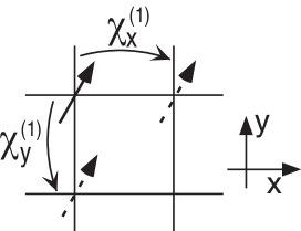
Figure 1: Fermion hopping amplitudes, $\chi_{x}^{(1)}$ and $\chi_{y}^{(1)}$, central quantities in this paper. They are abbreviated to $\chi_{x}$ and $\chi_{y}$, respectively.

Following the previous procedure[13], we introduce mean fields: $\chi_{\tau}^{(l)}\equiv\left<\sum_{\sigma}f_{i\,\sigma}^{\dagger}f_{i+\tau\,\sigma}\right>$, $\left<b_{i}^{\dagger}b_{i+\tau}\right>$ and $\Delta_{\tau}^{(1)}\equiv\left<f_{i\,\uparrow}f_{i+\tau\,\downarrow}-f_{i\,\downarrow}f_{i+\tau\,\uparrow}\right>$, where each is taken to be a real constant independent of lattice coordinates, but is allowed its dependence on the bond direction $\mbox{\boldmath$\tau$}=\mbox{\boldmath$r$}_{j}-\mbox{\boldmath$r$}_{i}$ (see Fig. 1). Also, the local constraint eq. (2) is loosened to a global one, $\sum_{i}\left(\sum_{\sigma}f_{i\,\sigma}^{\dagger}f_{i\,\sigma}+b_{i}^{\dagger}b_{i}\right)=N$ with $N$ being the total number of lattice sites. We then decouple the Hamiltonian eq. (1) to obtain

$$H_{\rm MF}=\sum_{\mbox{\boldmath$k$},\,\sigma}\xi_{\mbox{\boldmath$k$}}f_{\mbox{\boldmath$k$}\,\sigma}^{\dagger}f_{\mbox{\boldmath$k$}\,\sigma}+\sum_{\mbox{\boldmath$k$}}\left(\Delta_{\mbox{\boldmath$k$}}f_{-\mbox{\boldmath$k$}\,\downarrow}^{\dagger}f_{\mbox{\boldmath$k$}\,\uparrow}^{\dagger}+\Delta_{\mbox{\boldmath$k$}}^{\ast}f_{\mbox{\boldmath$k$}\,\uparrow}f_{-\mbox{\boldmath$k$}\,\downarrow}\right),$$ (3)

$$\xi_{\mbox{\boldmath$k$}}=-2\sum_{l,\,\tau}F_{\tau}^{(l)}\cos k_{\tau}-\mu\;,$$ (4)

$$F_{\tau}^{(l)}=t\!\,^{(l)}\left<b_{i}^{\dagger}b_{i+\tau}\right>+\frac{3}{8}J\chi_{\tau}^{(l)}\;\delta_{l,\,1}\;,$$ (5)

$$\Delta_{\mbox{\boldmath$k$}}=-\frac{3}{4}J\left(\Delta_{x}^{(1)}\cos k_{x}+\Delta_{y}^{(1)}\cos k_{y}\right),$$ (6)

where $\mu$ is the chemical potential, $\delta_{l,1}$ is the Kronecker’s delta, and $k_{\tau}=k_{x}$ or $k_{y}$ for $l=1$, $k_{\tau}=k_{x}+k_{y}$ or $k_{x}-k_{y}$ for $l=2$ and $k_{\tau}=2k_{x}$ or $2k_{y}$ for $l=3$. We approximate bosons to be Bose-condensed and neglect the kinetic term for bosons in eq. (3). This approximation will be reasonable at low temperature, and leads to $\left<b_{i}^{\dagger}b_{i+\tau}\right>\approx\delta$ where $\delta$ is the hole density. It is to be noted that we do not assume four-fold symmetry, $\chi_{x}^{(1)}=\chi_{y}^{(1)}$ and $\left|\Delta_{x}^{(1)}\right|=\left|\Delta_{y}^{(1)}\right|$, which was assumed previously[13]. In the following, we abbreviate $\chi_{\tau}^{(1)}$ and $\Delta_{\tau}^{(1)}$ to $\chi_{\tau}$ and $\Delta_{\tau}$, respectively.

3 Results

In §3.1 and §3.2, focusing our attention on the LSCO systems, we set the parameters as $t^{(1)}/J=4$, $t^{(2)}/t^{(1)}=-1/6$ and $t^{(3)}/t^{(1)}=0$, and determine the mean fields by minimizing the free energy. These parameters reproduce the observed FS at $\delta=0.30$[10] in LSCO[14]. We also study with the other parameter choice in §3.3.

3.1 Isotropic $t$-$J$ model

3.1.1 Numerical calculations

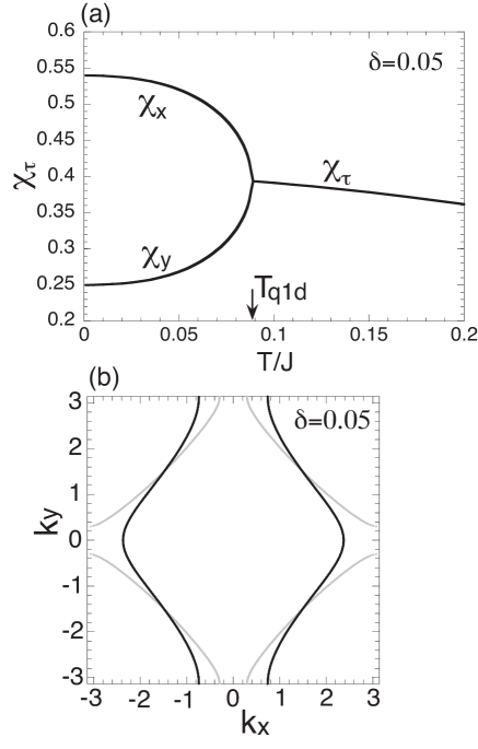
Figure 2: (a) $T$-dependence of $\chi_{\tau}$ in the isotropic $t$-$J$ model with the constraint $\Delta_{\tau}=0$. The four-fold symmetry is broken spontaneously below $T_{\rm q1d}$, that is $\chi_{x}\neq\chi_{y}$. (b) Fermi surface for $T>T_{\rm q1d}$ (gray line) and that for $T<T_{\rm q1d}$ (solid line).

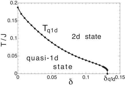
Figure 3: $\delta$-dependence of $T_{\rm q1d}$ in the isotropic $t$-$J$ model with the constraint $\Delta_{\tau}=0$.                 

We first show the numerical results obtained under the constraint $\Delta_{\tau}=0$. Figure 2(a) shows $\chi_{\tau}$ as a function of temperature $T$. A second-order phase transition takes place at $T=T_{\rm q1d}$, below which the four-fold symmetry of $\chi_{\tau}$ is broken spontaneously, that is $\chi_{x}\neq\chi_{y}$. The 2d FS (gray line in Fig. 2(b)) at high temperature changes into the q-1d FS (solid line) for $T<T_{\rm q1d}$. Figure 3 shows $T_{\rm q1d}$ as a function of $\delta$. The q-1d state is realized below the critical doping rate, $\delta_{\rm q1d}\approx 0.13$. The jump of $T_{\rm q1d}$ at $\delta_{\rm q1d}$ indicates a weak first-order phase transition at $T=0$ as a function of $\delta$.

When we remove the constraint $\Delta_{\tau}=0$, the 2d $d$-RVB state ($\Delta_{x}=-\Delta_{y}$) sets in before the q-1d instability occurs, and the q-1d state does not appear.

3.1.2 Ginzburg-Landau analysis

To see the origin of the q-1d state and its competition with the $d$-RVB, we examine a Ginzburg-Landau (GL) free energy. Under the constraint $\Delta_{\tau}=0$, we vary $\chi_{\tau}$ and $\mu$ infinitesimally around the isotropic 2d state, $\chi_{0}$ and $\mu_{0}$, keeping $\delta$ fixed: $\chi_{x}=\chi_{0}+\delta\!\chi$, $\chi_{y}=\chi_{0}-\delta\!\chi$, and $\mu=\mu_{0}+\delta\!\mu$. Up to the second order in $\delta\!\chi$ and $\delta\!\mu$, we estimate the dominant terms in the GL free energy as

$$F-F_{0}\sim\frac{3J}{4}(1-a)(\delta\!\chi)^{2}.$$ (7)

Here $F_{0}$ is the free energy in the isotropic 2d state and

$$a=\frac{3J}{4}\frac{1}{N}\sum_{\mbox{\boldmath$k$}}\left(-\frac{\partial n_{F}}{\partial\xi_{\mbox{\boldmath$k$}}}\right)\left(\cos k_{x}-\cos k_{y}\right)^{2}>0\;,$$ (8)

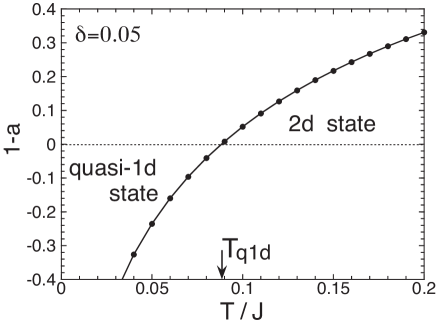
Figure 4: GL coefficient, $1-a$, for several $T$ at $\delta=0.05$ under the constraint $\Delta_{\tau}=0$. It becomes negative below $T_{\rm q1d}\approx 0.09J$, signaling an instability toward the quasi-1d state.

where $n_{F}$ is the Fermi-Dirac distribution function. The GL coefficient, $1-a$, at $\delta=0.05$ is shown in Fig. 4 as a function of $T$. It becomes negative below $T_{\rm q1d}\approx 0.09J$, signaling an instability toward the q-1d state. This value of $T_{\rm q1d}$ is the same as that shown in Fig. 2(a), which confirms that the q-1d instability is controlled by $a$.

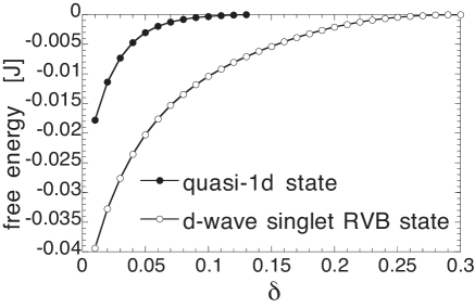
Figure 5: Free energy at $T=0.01J$ of the quasi-1d state and of the $d$-wave singlet RVB ($d$-RVB) state, relative to that of the isotropic 2d state without the $d$-RVB.

Since in eq. (8), the factor $-\frac{\partial n_{F}}{\partial\xi_{\mbox{\boldmath$k$}}}$ limits $k$ to a region close to the FS, and the form factor $(\cos k_{x}-\cos k_{y})^{2}$ takes maxima at points $(\pi,\,0)$ and $(0,\,\pi)$, the condensation energy for the q-1d state comes mainly from fermions on the FS near $(\pi,\,0)$ and $(0,\,\pi)$. The same energetics holds for the $d$-RVB state also. In this sense, the q-1d state competes with the $d$-RVB state. Figure 5 shows that the condensation energy is larger for the latter. This is why the $d$-RVB state has overcome the q-1d state in our numerical calculation.

3.2 Anisotropic $t$-$J$ model

Having seen that the q-1d state has free energy higher than the $d$-RVB state, we next ask a question: is there any perturbation which favors the q-1d state relative to the $d$-RVB state and stabilizes the q-1d state, or at least the coexistence with the $d$-RVB state? We here show that a small spatial anisotropy in $t^{(1)}$ and $J$ exposes the q-1d instability which has been hidden behind the $d$-RVB, and brings about the coexistence with the $d$-RVB state. As an origin of this anisotropy, we consider the low-temperature tetragonal (LTT) structure and introduce as[15, 16]

$$t_{x}^{(1)}=t^{(1)},\quad t_{y}^{(1)}=t^{(1)}(1-3.78\tan^{2}\theta),$$ (9)

$$J_{x}=J,\quad J_{y}=J(1-2\cdot 3.78\tan^{2}\theta),$$ (10)

where $\theta$ is a tilting angle of the CuO₆ octahedra and the subscripts, $x$ and $y$, indicate the bond direction. (In §4.1.1, we will discuss a possible origin of this anisotropy in LSCO whose crystal structure is the low-temperature orthorhombic (LTO).) Taking $\theta=5^{\circ}$[17], namely $t_{y}^{(1)}/t_{x}^{(1)}\approx 0.97$ and $J_{y}/J_{x}\approx 0.94$, we determine the mean fields without the constraint $\Delta_{\tau}=0$.

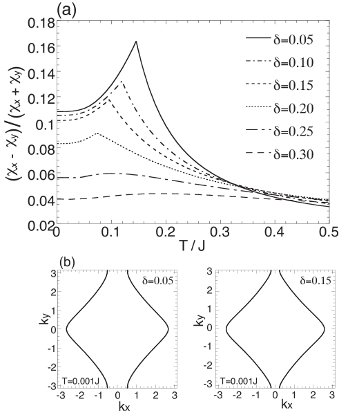
Figure 6: (a) $T$-dependence of the degree of the anisotropy, $\frac{\chi_{x}-\chi_{y}}{\chi_{x}+\chi_{y}}$, for several choices of $\delta$ in the anisotropic $t$-$J$ model with $\theta=5^{\circ}$. (b) Quasi-1d Fermi surfaces in a state coexistent with the $d$-RVB at $T=0.001J$ for $\delta=0.05$ and $0.15$. The Fermi surface is defined by $\xi_{\mbox{\boldmath$k$}}=0$, although the fermion dispersion is given by $E_{\mbox{\boldmath$k$}}=\sqrt{\xi_{\mbox{\boldmath$k$}}^{2}+|\Delta_{\mbox{\boldmath$k$}}|^{2}}$ in the coexistent state.

Figure 6(a) shows the degree of the anisotropy, $\frac{\chi_{x}-\chi_{y}}{\chi_{x}+\chi_{y}}$, as a function of $T$. For $\delta$$\stackrel{{\scriptstyle<}}{{\sim}}$$0.20$, the anisotropy is largely enhanced as decreasing $T$ and after showing a cusp at $T_{\rm RVB}$, onset temperature of the $d$-RVB, it decreases but approaches to a still enhanced value as $T\rightarrow 0$. The degree of the anisotropy at $T\sim 0.5J$ hardly depends on $\delta$ and hence can be solely due to the given anisotropy in $t^{(1)}$ and $J$. The enhanced anisotropy at lower temperature comes from the intrinsic q-1d instability, whose competition with the $d$-RVB makes the cusp at $T_{\rm RVB}$. This competition also suppresses the value of $T_{\rm RVB}$ about $6\sim 8\%$ compared to that of $T_{\rm RVB}$ for the (pure) $d$-RVB state realized in the isotropic $t$-$J$ model. Despite the competition, a still enhanced anisotropy survives at $T=0$ and becomes smaller as increasing $\delta$. Figure 6(b) shows the FSs at $T=0.001J$ for $\delta=0.05$ and $0.15$, which are q-1d. For $\delta$$\stackrel{{\scriptstyle>}}{{\sim}}$$0.25$, the value of $\frac{\chi_{x}-\chi_{y}}{\chi_{x}+\chi_{y}}$ does not depend on $T$ appreciably. This behavior qualitatively different from that for $\delta$$\stackrel{{\scriptstyle<}}{{\sim}}$$0.20$ can be understood as coming from the fact that the intrinsic q-1d instability is limited to $\delta$$\stackrel{{\scriptstyle<}}{{\sim}}$$\delta_{\rm q1d}\approx 0.13$ in the isotropic $t$-$J$ model as found under the constraint $\Delta_{\tau}=0$. In this sense, the value of $\delta_{\rm q1d}$ is a rough measure of the extent of $\delta$ where the intrinsic q-1d instability appears in the anisotropic $t$-$J$ model.

We note that in the coexistent state an extended $s$-wave component, $\Delta_{s}$, mixes into the $d$-wave component, $\Delta_{d}$:

$$\Delta_{d}=\frac{1}{2}\left|\Delta_{x}-\Delta_{y}\right|,$$ (11)

$$\Delta_{s}=\frac{1}{2}\left|\Delta_{x}+\Delta_{y}\right|.$$ (12)

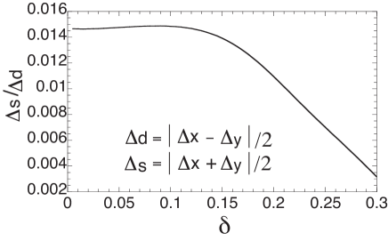
Figure 7: Relative magnitude of the extended $s$-wave component, $\Delta_{s}/\Delta_{d}$, as a function of $\delta$ at $T=0.001J$. The $\theta$ is set to $5^{\circ}$ in the anisotropic $t$-$J$ model.

Figure 7 shows that the mixing is about 1.5% for $\delta$$\stackrel{{\scriptstyle<}}{{\sim}}$$0.15$. This small $s$-wave ratio does not shift the Fermi point ($d$-wave node) appreciably from the symmetry axis $k_{y}=\pm k_{x}$; its shift is less than $\sim 0.1\%$ of the 1st Brillouin zone.

3.3 Band parameter dependence

Next we examine the band parameter dependence of the q-1d instability. Taking $t^{(1)}/J=4$ in common, we consider the following three cases, which reproduce different types of the FS: (a) $t^{(2)}/t^{(1)}=-1/6$, $t^{(3)}/t^{(1)}=0$, (b) $t^{(2)}/t^{(1)}=0$, $t^{(3)}/t^{(1)}=0$, and (c) $t^{(2)}/t^{(1)}=-1/6$, $t^{(3)}/t^{(1)}=1/5$. The case (a) is just what we have considered, and will be used as a reference below.

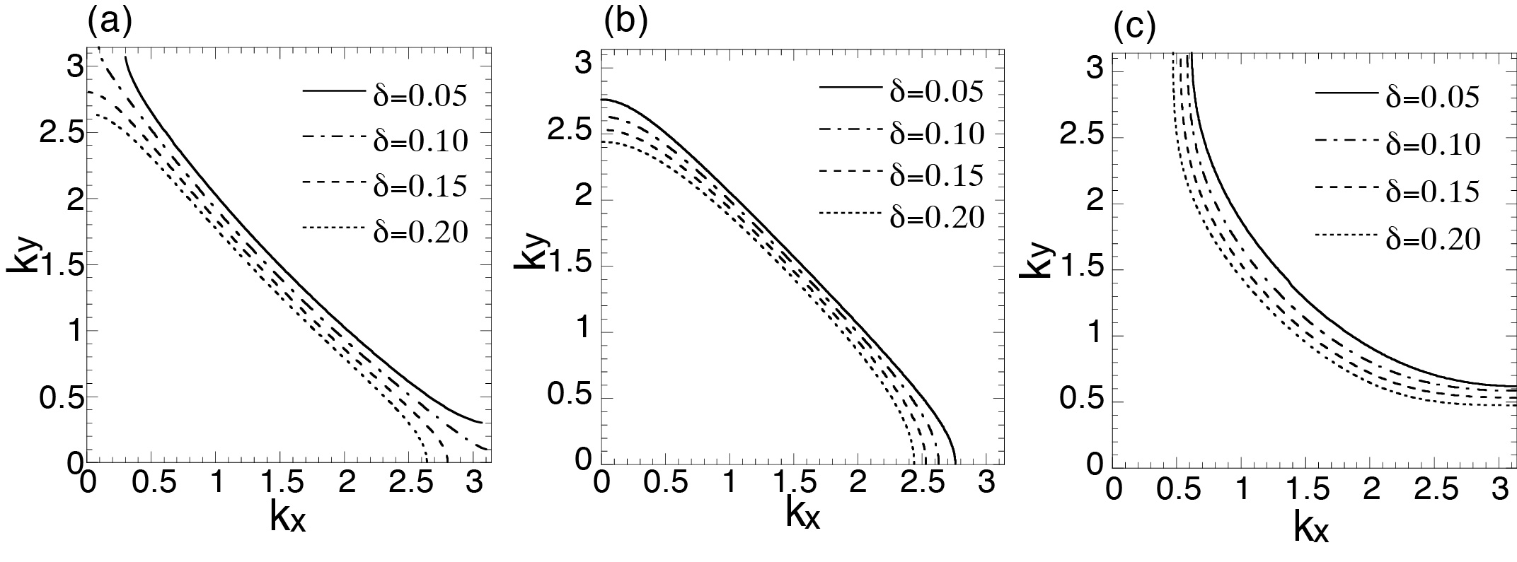
Figure 8: Fermi surfaces at $T=0.2J$ in the isotropic $t$-$J$ model: (a) $t^{(2)}/t^{(1)}=-1/6$, $t^{(3)}/t^{(1)}=0$, (b) $t^{(2)}/t^{(1)}=0$, $t^{(3)}/t^{(1)}=0$, and (c) $t^{(2)}/t^{(1)}=-1/6$, $t^{(3)}/t^{(1)}=1/5$. They have a four-fold symmetry.

Figure 8 shows the FSs for each case at high temperature ($T=0.2J$) in the isotropic $t$-$J$ model. The $\delta$-dependence of $T_{\rm q1d}$ obtained under the constraint $\Delta_{\tau}=0$ is shown in Fig. 9. The value of $\delta_{\rm q1d}$ depends strongly on the band parameters, and is about (a) 0.13, (b) 0.075, and (c) 0.04, respectively. The q-1d state is most favored for case (a) because, as shown in Fig. 8, the FS is located near $(\pi,\,0)$ and $(0,\,\pi)$ compared to the other cases, especially at low $\delta$. Although the realistic $\delta$ for high-$T_{\rm c}$ cuprates may be at most $0.30$, we note for case (c) that the q-1d instability occurs again at $\delta\approx 0.46$-$0.48$ with $T_{\rm q1d}$$\stackrel{{\scriptstyle<}}{{\sim}}$$0.008J$. This is because the FS passes near the points $(\pi,\,0)$ and $(0,\,\pi)$ around $\delta\sim 0.45$.

On the other hand, when we remove the constraint $\Delta_{\tau}=0$ in the isotropic $t$-$J$ model, the $d$-RVB state completely overcomes the q-1d state. This feature is common to the three cases.

In the anisotropic $t$-$J$ model with $\theta=5^{\circ}$, we observe that the anisotropy $\frac{\chi_{x}-\chi_{y}}{\chi_{x}+\chi_{y}}$ forms the cusp structure as a function of $T$ in a region below $\delta\sim$ (a) $0.20$, (b) $0.15$, and (c) $0.10$, respectively. This band parameter dependence reflects the different value of $\delta_{\rm q1d}$ for each case. For case (c), however, the cusp structure reappears above $\delta\sim 0.35$. In addition, the value of $\frac{\chi_{x}-\chi_{y}}{\chi_{x}+\chi_{y}}$ at $T\approx 0$ increases with $\delta$ above $\delta\approx 0.15$-$0.20$ while it decreases with $\delta$ for the other cases as shown in Fig. 6(a). These different behaviors for case (c) can be understood as due to the proximity of the FS to the points $(\pi,\,0)$ and $(0,\,\pi)$ at the higher $\delta$.

4 Discussion

4.1 Comparison with experiments

Now we discuss a relevance of the present q-1d state to high-$T_{\rm c}$ cuprates. The constraint $\Delta_{\tau}=0$ should be removed in the discussion. The results in the preceding section indicate two important factors: (i) a spatial anisotropy in $t^{(1)}$ and $J$, and (ii) the values of $t^{(1)}$, $t^{(2)}$ and $t^{(3)}$. The former has effectively exposed the q-1d instability which was hidden behind the $d$-RVB state as shown in Fig. 6; the extent of the ‘stability region’ of the q-1d state can be roughly measured by the value of $\delta_{\rm q1d}$ as discussed in §3.2 and §3.3. This value of $\delta_{\rm q1d}$ strongly depends on the latter factor.

4.1.1 La_2-xSr_xCuO₄

For LSCO, we take band parameters, $t^{(1)}/J=4,t^{(2)}/t^{(1)}=-1/6$ and $t^{(3)}/t^{(1)}=0$. This choice reproduces the observed FS at $\delta=0.30$[10] in the isotropic $t$-$J$ model.

We first discuss La_1.6-xNd_0.4Sr_xCuO₄, assuming the same band parameters as those of LSCO. The crystal structure is LTT or $Pccn$ (an intermediate structure between LTO and LTT) at temperatures below $T_{\rm d2}$ in a range $0$$\stackrel{{\scriptstyle<}}{{\sim}}$$\delta$$\stackrel{{\scriptstyle<}}{{\sim}}$$0.30$[23, 24], and the static spatial anisotropy is present in $t^{(1)}$ and $J$. We thus expect the realization of the static q-1d state below $T_{\rm d2}$ or its coexistence with the $d$-RVB. Even above $T_{\rm d2}$, the dynamical q-1d fluctuations is expected as discussed below.

On the other hand, for LSCO the crystal structure is LTO and hence allows no static spatial anisotropy in $t^{(1)}$ and $J$. The use of the results for the anisotropic $t$-$J$ model obtained in the preceding section is thus not justified. However, noting the existence of the Z-point soft phonon mode associated with the structural phase transition from LTO to LTT at low temperature in a range $0\leq\delta\leq 0.18$[18, 19, 20], we expect a spatial anisotropy in $t^{(1)}$ and $J$ within a time scale $\omega_{\rm ph}^{-1}$ and a spatial scale of the correlation length of the LTT fluctuation, where $\hbar\omega_{\rm ph}=1$-$2$ meV is the energy of the Z-point soft phonon mode (called as the ‘LTT-phonon’ below). To estimate the value of $\theta$, we recall an experimental indication[21] that the LTT fluctuation around the LTO structure occurs as a simple rotation of the CuO₆ tilting direction in the plane, namely, from e.g. [110] to e.g. [100] (tetragonal notation), as successfully modeled by a classical XY model. This means that the magnitude of the (instantaneous) LTT distortion can be as large as that of the (time-averaged) LTO distortion. Since the tilting angle in the LTO structure is $\theta\approx 2$-$5^{\circ}$ for $\delta<0.18$[17], our choice of $\theta=5^{\circ}$ for the LTT distortion will be reasonable in magnitude. Taken these, we propose that in LSCO with the ‘LTT-phonon’ the q-1d state (or its coexistence with the $d$-RVB) is realized as dynamical fluctuations within time scales shorter than $\omega_{\rm ph}^{-1}$. Since the CuO₆ tilting pattern of the ‘LTT-phonon’ alternates between the $x$- and $y$-directions along the $c$-axis, the q-1d state (or precisely, q-1d fluctuations) will also have the same alternate structure (or alternate correlations) along the $c$-axis.

Because of the dynamical nature of the q-1d state in the LTO structure, the experimental observation of the proposed q-1d state will depend on probes. High-energy probes ($\omega$$\stackrel{{\scriptstyle>}}{{\sim}}$$\omega_{\rm ph}$), such as ARPES and inelastic neutron scattering, will observe an instantaneous q-1d state, while low-energy probes ($\omega\ll\omega_{\rm ph}$), such as NMR and $\mu$SR, will observe a time-averaged state, which is 2d-like in each CuO₂ plane. We have interpreted the data from the former class (ARPES and neutron) in terms of the present q-1d picture[9]. Among others, we can fit the observed FS segments[10] semiquantitatively with the q-1d FSs determined in the present anisotropic $t$-$J$ model with $\theta=5^{\circ}$ at low temperature $(T\ll J)$.

We note a recent report[22] that LSCO has the $Pccn$ structure at low temperature at $\delta=0.115$. According to the scenario so far described, the q-1d state can become static even in LSCO. In the reverse way, we may argue that the present coupling between (spin) fermions and phonons via the anisotropy in $t^{(1)}$ and $J$ is the origin of the $Pccn$ structure when the q-1d fluctuations are frozen in the LTO structure.

4.1.2 YBa₂Cu₃O_6+y

Following the previous report[13], we take $t^{(1)}/J=4,t^{(2)}/t^{(1)}=-1/6$ and $t^{(3)}/t^{(1)}=1/5$. For $y$$\stackrel{{\scriptstyle>}}{{\sim}}$$0.4$, CuO chains order along the $b$-axis accompanying the orthorhombicity $(b-a)/(b+a)$$\stackrel{{\scriptstyle<}}{{\sim}}$$1$% in the in-plane lattice constants $a$ and $b$[25]. (The crystal structure is tetragonal for $y$$\stackrel{{\scriptstyle<}}{{\sim}}$$0.4$.) A weak coupling to the CuO chain band will cause the spatial anisotropy, $t_{y}^{(1)}/t_{x}^{(1)}>1$, which will be, however, reduced by the orthorhombicity whose effect is estimated as[26] $t_{y}^{(1)}/t_{x}^{(1)}\propto(\frac{a}{b})^{3.5}<1$. The resulting anisotropy may be comparable to or less than that in LSCO. In addition, with the present choice of band parameters the degree of the intrinsic q-1d instability is very small compared to the case of LSCO (Fig. 9). Figure 10 indeed shows that the FSs for $\delta=0.05$ and $0.30$ remain almost 2d at $T=0.01J$ in the anisotropic $t$-$J$ model with $\theta=5^{\circ}$. (Such a parametrization in terms of $\theta$ is, of course, not appropriate for YBCO, where there is no ‘tilting’. Hence, the use of $\theta$ is just for convenience in a comparison with the case of LSCO.) Therefore YBCO system is not effective in realizing the q-1d state, and instead the 2d $d$-RVB state will be realized at low temperature. This picture is consistent with the ARPES data[27] in that the observed FS at $T\sim 20$K is 2d hole-like centered at $(\pi,\,\pi)$.

4.2 Possible charge inhomogeneity

We have assumed that the charge (boson) distribution is homogeneous. If we relax this restriction, it is possible that the charge distribution becomes inhomogeneous and especially takes a q-1d structure in the state with the q-1d FS. In this connection, the ‘charge stripe’ picture[1, 2] will be interesting. These aspects, including the possible competition with the Bose condensation or superconductivity, are left to future studies.

4.3 Nearest neighbor Coulomb interaction

As seen in §3.2, a small perturbation to the original isotropic $t$-$J$ model has exposed its intrinsic q-1d instability. From the same viewpoint, the role of the n.n. Coulomb interaction, $V$, will be interesting. Our preliminary calculation in the isotropic $t$-$J$ model with $t^{(1)}/J=4$, $t^{(2)}/t^{(1)}=-1/6$ and $t^{(3)}/t^{(1)}=0$ shows that a reasonable value of $V$ stabilizes the coexistence of the q-1d state with the $d$-RVB below $\delta\sim 0.10$[28]. Therefore, in realizing the q-1d state, effects of $V$ are cooperative with those of the small spatial anisotropy in $t^{(1)}$ and $J$, and the former tends to freeze the q-1d fluctuation due to the ‘LTT-phonon’.

5 Summary

We have found within the slave-boson mean field approximation that the 2d $t$-$J$ model has an intrinsic instability toward forming a q-1d FS. This q-1d instability is driven mainly by fermions on the FS near $(\pi,\,0)$ and $(0,\,\pi)$, and thus competes with the $d$-RVB. For a realistic parameter choice, the $d$-RVB state completely overcomes the q-1d state. However, we have shown that a small spatial anisotropy in $t^{(1)}$ and $J$ exposes the q-1d instability which has been hidden behind the $d$-RVB state, and brings about the coexistence with the $d$-RVB. We have argued that this coexistence can be realized in LSCO systems.

Acknowledgements. We thank Professor H. Fukuyama for his continual encouragement. H. Y. also thanks Professor T. Fujita for informing him of ref. 22. This work is supported by a Grant-in-Aid for Scientific Research from Monbusho.

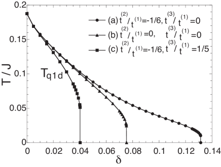
Figure 9: $T_{\rm q1d}$ as a function of $\delta$ in the isotropic $t$-$J$ model under the constraint $\Delta_{\tau}=0$: (a) $t^{(2)}/t^{(1)}=-1/6$, $t^{(3)}/t^{(1)}=0$, (b) $t^{(2)}/t^{(1)}=0$, $t^{(3)}/t^{(1)}=0$, and (c) $t^{(2)}/t^{(1)}=-1/6$, $t^{(3)}/t^{(1)}=1/5$. The values of $\delta_{\rm q1d}$ are about (a) 0.13, (b) 0.075, and (c) 0.04, respectively.

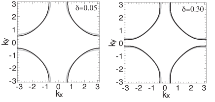
Figure 10: Fermi surfaces for $\delta=0.05$ and $0.30$ at $T=0.01J$ in the anisotropic $t$-$J$ model with $\theta=5^{\circ}$ (solid line) and $0^{\circ}$ (gray line). The band parameter is taken as $t^{(1)}/J=4$, $t^{(2)}/t^{(1)}=-1/6$ and $t^{(3)}/t^{(1)}=1/5$, appropriate to YBCO. The Fermi surface is defined by $\xi_{\mbox{\boldmath$k$}}=0$, although the fermion dispersion is given by $E_{\mbox{\boldmath$k$}}=\sqrt{\xi_{\mbox{\boldmath$k$}}^{2}+|\Delta_{\mbox{\boldmath$k$}}|^{2}}$.

References

- [1] J. M. Tranquada, B. J. Sternlieb, J. D. Axe, Y. Nakamura and S. Uchida: Nature 375 (1995) 561.
- [2] J. M. Tranquada, J. D. Axe, N. Ichikawa, Y. Nakamura, S. Uchida and B. Nachumi: Phys. Rev. B 54 (1996) 7489.
- [3] J. M. Tranquada, J. D. Axe, N. Ichikawa, A. R. Moodenbaugh, Y. Nakamura and S. Uchida: Phys. Rev. Lett. 78 (1997) 338.
- [4] S. R. White and D. J. Scalapino: Phys. Rev. Lett. 80 (1998) 1272.
- [5] S. R. White and D. J. Scalapino: Phys. Rev. Lett. 81 (1998) 3227.
- [6] S. R. White and D. J. Scalapino: cond-mat/9907243.
- [7] C. S. Hellberg and E. Manousakis: Phys. Rev. Lett. 83 (1999) 132.
- [8] C. S. Hellberg and E. Manousakis: cond-mat/9910142.
- [9] H. Yamase and H. Kohno: J. Phys. Soc. Jpn. 69 (2000) 332; H. Yamase, H. Kohno and H. Fukuyama: Physica B 284-288 (2000) 1375.
- [10] A. Ino, C. Kim, T. Mizokawa, Z.-X. Shen, A. Fujimori, M. Takaba, K. Tamasaku, H. Eisaki and S. Uchida: J. Phys. Soc. Jpn. 68 (1999) 1496.
- [11] K. Yamada, C. H. Lee, K. Kurahashi, J. Wada, S. Wakimoto, S. Ueki, H. Kimura, Y. Endoh, S. Hosoya, G. Shirane, R. J. Birgeneau, M. Greven, M. A. Kastner and Y. J. Kim: Phys. Rev. B 57 (1998) 6165.
- [12] H. Yamase, H. Kohno and H. Fukuyama: to appear in Physica C.
- [13] T. Tanamoto, H. Kohno and H. Fukuyama: J. Phys. Soc. Jpn. 62 (1993) 717.
- [14] We consider to be equal to the Sr2+ content, .
- [15] B. Normand, H. Kohno and H. Fukuyama: Phys. Rev. B 53 (1996) 856.
- [16] H. Yamase, H. Kohno, H. Fukuyama and M. Ogata: J. Phys. Soc. Jpn. 68 (1999) 1082.
- [17] P. G. Radaelli, D. G. Hinks, A. W. Mitchell, B. A. Hunter, J. L. Wagner, B. Dabrowski, K. G. Vandervoort, H. K. Viswanathan and J. D. Jorgensen: Phys. Rev. B 49 (1994) 4163.
- [18] T. R. Thurston, R. J. Birgeneau, D. R. Gabbe, H. P. Jenssen, M. A. Kastner, P. J. Picone, N. W. Preyer, J. D. Axe, P. Böni, G. Shirane, M. Sato, K. Fukuda and S. Shamoto: Phys. Rev. B 39 (1989) 4327.
- [19] C. H. Lee, K. Yamada, M. Arai, S. Wakimoto, S. Hosoya and Y. Endoh: Physica C 257 (1996) 264.
- [20] H. Kimura, K. Hirota, C. H. Lee, K. Yamada and G. Shirane: cond-mat/9908217.
- [21] J. D. Axe, A. H. Moudden, D. Hohlwein, D. E. Cox, K. M. Mohanty, A. R. Moodenbaugh and Youwen Xu: Phys. Rev. Lett. 62 (1989) 2751.
- [22] S. Sakita, F. Nakamura, T. Suzuki and T. Fujita: J. Phys. Soc. Jpn. 68 (1999) 2755.
- [23] M. K. Crawford, R. L. Harlow, E. M. McCarron, W. E. Farneth, J. D. Axe, H. Chou and Q. Huang: Phys. Rev. B 44 (1991) 7749.
- [24] B. Büchner, M. Breuer, A. Freimuth and A. P. Kampf: Phys. Rev. Lett. 73 (1994) 1841.
- [25] J. D. Jorgensen, B. W. Veal, A. P. Paulikas, L. J. Nowicki, G. W. Crabtree, H. Claus and W. K. Kwok: Phys. Rev. B 41 (1990) 1863.
- [26] W. A. Harisson: Electronic Structure and the Properties of Solids (Freeman, New York, 1980).
- [27] M. C. Schabel, C.-H. Park, A. Matsuura, Z.-X. Shen, D. A. Bonn, Ruixing Liang and W. N. Hardy: Phys. Rev. B 57 (1998) 6107.
- [28] H. Yamase and H. Kohno: in preparation.