A geometric approximation of $\delta$-interactions by Neumann Laplacians

Abstract.

We demonstrate how to approximate one-dimensional Schrödinger operators with $\delta$-interaction by a Neumann Laplacian on a narrow waveguide-like domain. Namely, we consider a domain consisting of a straight strip and a small protuberance with “room-and-passage” geometry. We show that in the limit when the perpendicular size of the strip tends to zero, and the room and the passage are appropriately scaled, the Neumann Laplacian on this domain converges in (a kind of) norm resolvent sense to the above singular Schrödinger operator. Also we prove Hausdorff convergence of the spectra. In both cases estimates on the rate of convergence are derived.

1. Introduction

Schrödinger operators with potentials supported on a discrete set of points have attracted considerable attention over several past decades due to numerous applications in different fields of science and engineering. In particular, such operators serve as solvable models in quantum mechanics. The term “solvable” reflects the fact that their mathematical and physical quantities, like spectrum, eigenfunctions and resonances, can be calculated in many cases explicitly. We refer to the monograph [1] for a comprehensive introduction to this topic. Note that in the literature such models are also called Schrödinger operators with point interactions.

Investigation of these operators was originated by the famous Kronig-Penney model [18], concerning a non-relativistic electron moving in a fixed crystal lattice. Its mathematical representation is a one-dimensional Schrödinger operator with a singular potential supported at $\mathbb{Z}=\{0,\pm 1,\pm 2,\dots\}$:

$$-\frac{\,\mathrm{d}^{2}}{\,\mathrm{d}x^{2}}+\gamma\sum_{z\in\mathbb{Z}}\delta(\cdot-z),$$ (1.1)

where $\delta(\cdot-z)$ denotes the Dirac delta-function supported at $z$, and where $\gamma\in\mathbb{R}$ is the strength of the $\delta$-interaction. The formal expression (1.1) can be realized as a self-adjoint operator in $\mathsf{L}^{2}(\mathbb{R})$: the action of this operator is given by $-(f\restriction_{\mathbb{R}\setminus\mathbb{Z}})^{\prime\prime}$, its domain consists of $f\in\mathsf{H}^{2}(\mathbb{R}\setminus\mathbb{Z})$ satisfying the following conditions at $z\in\mathbb{Z}$:

$$f(z-0)=f(z+0),\quad f^{\prime}(z+0)-f^{\prime}(z-0)=\gamma f(z\pm 0).$$ (1.2)

One says that the conditions (1.2) correspond to a $\delta$-interaction with strength $\gamma$ supported at the point $z$.

In the present paper we wish to contribute to the understanding of ways how Schrödinger operators with $\delta$-interactions can be approximated by differential operators with regular coefficients. In what follows, we restrict ourselves to a Schrödinger operator on an open interval $\Omega_{0}$ (bounded or not) with a single $\delta$-interaction with strength $\gamma$ supported at $0$; we denote this operator by ${\mathcal{A}}_{0}$. The obtained results can easily be extended to Schrödinger operators with finitely and even countably many $\delta$-interactions, see Section 5.

One way of approximation is given by a sequence of Schrödinger operators with smooth $\delta$-like potentials, see e.g. [1, Sec. 1.3.2]. In the present work we discuss another approach, in which the desired $\delta$-interaction is generated by geometry. Namely, we construct a waveguide-like domain $\Omega_{\varepsilon}$ such that its Neumann Laplacian ${\mathcal{A}}_{\varepsilon}$ converges (in a kind of norm-resolvent topology) to the desired operator ${\mathcal{A}}_{0}$ as the perpendicular size of the guide tends to zero. Since the approximating operator is non-negative (minus the Laplacian), we can only expect $\gamma\geq 0$ in the limit (in our convention, $\gamma\geq 0$ leads to a non-negative operator with $\delta$-interaction, see (2.9) for the corresponding form).

Figure 1. The waveguide $\Omega_{\varepsilon}$

The approximating domain will be a thickened version of $\Omega_{0}$ with a decoration near $0\in\Omega_{0}$ given by a small passage $P_{\varepsilon}$ and a larger (but shrinking) room $R_{\varepsilon}$ (see Figure 1). In particular, the room (a square with side length $b_{\varepsilon}=\varepsilon^{\beta}$) can be chosen to shrink arbitrarily slow ($\beta\in(0,1/2)$), and the passage of height $h_{\varepsilon}=\varepsilon^{\alpha}$ and width $d_{\varepsilon}=\gamma\varepsilon^{\alpha+1}$ can shrink arbitrarily fast ($\alpha>0$). Nevertheless, the area $\varepsilon^{2\beta}$ of the room $R_{\varepsilon}$ is still shrinking compared to the transversal shrinking rate $\varepsilon$ of the strip $S_{\varepsilon}$. The strength of the $\delta$-interaction is given by $\gamma=d_{\varepsilon}/(h_{\varepsilon}\varepsilon)$. Note that we can interpret the quotient of the width $d_{\varepsilon}$ and the height $h_{\varepsilon}$ of the passage as the (vertical) conductance of $P_{\varepsilon}$.

It is interesting to compare our results with the the case, when the room is joined directly to the strip near $0$ as on Figure 2. Such a geometrical configuration was considered in [19, 11] (see also [23] for a version with generalised norm resolvent convergence). The critical value $1/2$ (in dimension $2$) of the parameter $\beta$ appears here as well. Namely, if $\beta\in(0,1/2)$, then the limit operator is the direct sum of the Laplacian with Dirichlet boundary condition at $0$ (hence decouples) and the $0$ operator on a one-dimensional space as in our case. In both cases (Figure 1 and Figure 2) the room area decays slower than the transversal shrinking rate, which attracts particles and leads to an own state (at energy $0$). If the room is directly attached to the strip (Figure 2), then it prevents transport along the strip, while in the present situation (Figure 1) it leads to a repulsive (i.e. with $\gamma\geq 0$) interaction at $0$. Note that for the waveguide as on Figure 2 in the critical case $b_{\varepsilon}=\varepsilon^{1/2}$ the limiting operator is the Laplacian with another peculiar conditions at $0$ (see the so-called “borderline case” in [11] or[23]); these conditions resemble (1.2) with the coupling constant $\gamma$ being replaced by a quantity dependent on the spectral parameter.

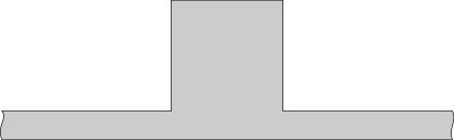
Figure 2.

Domains with attached protuberances with “room-and-passage” geometry are widely used in spectral theory in order to demonstrate various peculiar effects. For example, R. Courant and D. Hilbert [9] used such a domain as an example of a small perturbation breaking the continuity of eigenvalues of the Neumann Laplacian; see [3] for more details. In [14] such “rooms-and-passages” were used to construct a domain such that its Neumann Laplacian has prescribed essential spectrum (see also the overview [4] for more details). Homogenization problems in domains with corrugated “room-and-passage”-like boundary were studied in [7, 6]. Finally, various peculiar examples in the theory of Sobolev spaces are based on domains with such a geometry, see [2, 13, 10] and the monograph [20].

As the spaces change while passing to the limit $\varepsilon\to 0$, we use the framework of generalised norm resolvent convergence developed by the second author in [22] and [23]. We provide a self-contained presentation including a new proof of spectral convergence (cf. Theorem 3.5) in Section 3. As usual the generalised norm resolvent convergence is not much harder to show than other concepts such as versions of strong resolvent convergence used e.g. in homogenization theory [21, Chap. III], [27, Chap. XI].

Actually, our limit operator is not the Laplacian with $\delta$-interaction itself (as already mentioned above), but its direct sum with the null operator on a one-dimensional space. In Remark 2.3 we give some light on the appearance of this extra component.

The work is organized as follows. In Section 2 we set the problem and formulate the main results, Theorem 2.1 concerning the norm resolvent convergence and Theorem 2.2 concerning the spectral convergence. Note that we treat even more general operators $-\frac{\,\mathrm{d}^{2}}{\,\mathrm{d}x^{2}}+V_{0}+\delta(\cdot)$, where $V_{0}$ is a regular potential. In Section 3 we give two abstract results designed for studying convergence of operators in varying Hilbert spaces. Using them we prove the main results in Section 4. Finally, in Section 5 we discuss the case of countably many point interactions.

2. Setting of the problem and the main result

2.1. The waveguide $\Omega_{\varepsilon}$ and the operator ${\mathcal{A}}_{\varepsilon}$

Throughout the paper we denote points in $\mathbb{R}^{2}$ by $\mathbf{x}=(x_{1},x_{2})$. Let $\Omega_{0}=(\ell_{-},\ell_{+})\subset\mathbb{R}$ be an interval satisfying

$$-\infty\leq\ell_{-}<0<\ell_{+}\leq\infty.$$ (2.1)

Let $\varepsilon\in(0,\varepsilon_{0}]$ be a small parameter. We set

$$d_{\varepsilon}=\gamma\varepsilon^{\alpha+1},\quad h_{\varepsilon}=\varepsilon^{\alpha},\quad b_{\varepsilon}=\varepsilon^{\beta}\text{\quad with\quad}\alpha>0,\ 0<\beta<\frac{1}{2},\ \gamma>0.$$ (2.2)

Moreover, we claim $\varepsilon_{0}$ to be sufficiently small, namely

$$\varepsilon_{0}<\min\Bigl{\{}(2\gamma)^{-1/\alpha},|\ell_{-}|,\ell_{+}\Bigl{\}},\quad\varepsilon_{0}<\gamma^{-1/(\alpha+1-\beta)},\quad\text{and}\quad\varepsilon_{0}<\min\Bigl{\{}\gamma,\gamma^{-1}\Bigl{\}}.$$ (2.3)

The first assumption in (2.3) implies

$$d_{\varepsilon}\leq\frac{\varepsilon}{2}\qquad\text{and}\qquad[-\varepsilon,\varepsilon]\subset\Omega_{0},$$ (2.4)

the second one leads to

$$d_{\varepsilon}\leq b_{\varepsilon},$$ (2.5)

and the last one yields $|\ln\gamma|\leq|\ln\varepsilon|$ (it will be used in the proof of Lemma 4.3). Note that, since either $\gamma\leq 1$ or $\gamma^{-1}\leq 1$, one has $\varepsilon_{0}<1$. Finally, we introduce the domains

$$\begin{array}[]{llll}S_{\varepsilon}&=&\left\{\mathbf{x}\in\mathbb{R}^{2}:\ x_{1}\in\Omega_{0},\ x_{2}\in(-\varepsilon,0)\right\}&\text{(straight strip)},\\[5.69054pt] P_{\varepsilon}&=&\left\{\mathbf{x}\in\mathbb{R}^{2}:\ |x_{1}|<{\dfrac{d_{\varepsilon}}{2}},\ x_{2}\in(0,h_{\varepsilon})\right\}&\text{(passage)},\\[5.69054pt] R_{\varepsilon}&=&\left\{\mathbf{x}\in\mathbb{R}^{2}:\ |x_{1}|<\dfrac{b_{\varepsilon}}{2},\ x_{2}\in(h_{\varepsilon},h_{\varepsilon}+b_{\varepsilon})\right\}&\text{(room)},\end{array}$$

and the resulting domain $\Omega_{\varepsilon}$ given by

$$\Omega_{\varepsilon}=\operatorname{int}(\overline{S_{\varepsilon}\cup P_{\varepsilon}\cup R_{\varepsilon}})$$

(here $\operatorname{int}(\cdot)$ stands for the interior of a subset of $\mathbb{R}^{2}$). Due to (2.4)–(2.5) the geometry of $\Omega_{\varepsilon}$ is exactly as shown in Figure 1, i.e. the bottom part (respectively, the top part) of $\partial P_{\varepsilon}$ is contained in the top part of $\partial S_{\varepsilon}$ (respectively, the bottom part of $\partial R_{\varepsilon}$).

In the Hilbert space $\mathcal{H}_{\varepsilon}\coloneqq\mathsf{L}^{2}(\Omega_{\varepsilon})$ we introduce the sesquilinear form

$$\mathfrak{a}_{\varepsilon}[u,v]=\int_{\Omega_{\varepsilon}}\left(\nabla u(\mathbf{x})\cdot\overline{\nabla v(\mathbf{x})}+V_{\varepsilon}(\mathbf{x})u(\mathbf{x})\overline{v(\mathbf{x})}\right)\,\mathrm{d}\mathbf{x},\quad\operatorname{dom}(\mathfrak{a}_{\varepsilon})=\mathsf{H}^{1}(\Omega_{\varepsilon})$$ (2.6)

with a real-valued potential $V_{\varepsilon}\in\mathsf{L}^{\infty}(\Omega_{\varepsilon})$. This form is densely defined in $\mathsf{L}^{2}(\Omega_{\varepsilon})$, non-negative and closed, consequently [17, Theorem VI.2.1] there is a unique non-negative self-adjoint operator ${\mathcal{A}}_{\varepsilon}$ acting in $\mathsf{L}^{2}(\Omega_{\varepsilon})$ such that the domain inclusion $\operatorname{dom}({\mathcal{A}}_{\varepsilon})\subset\operatorname{dom}(\mathfrak{a}_{\varepsilon})$ and the equality

$$({\mathcal{A}}_{\varepsilon}u,v)_{\mathsf{L}^{2}(\Omega_{\varepsilon})}=\mathfrak{a}_{\varepsilon}[u,v],\quad\forall u\in\operatorname{dom}({\mathcal{A}}_{\varepsilon}),\,\,v\in\operatorname{dom}(\mathfrak{a}_{\varepsilon})$$

hold. Obviously, ${\mathcal{A}}_{\varepsilon}=-\Delta_{\Omega_{\varepsilon}}+V_{\varepsilon}$, where $\Delta_{\Omega_{\varepsilon}}$ is the Neumann Laplacian on $\Omega_{\varepsilon}$.

The main goal of this work is to describe the behavior of the resolvent and the spectrum of ${\mathcal{A}}_{\varepsilon}$ as $\varepsilon\to 0$. In the next subsection we introduce the anticipated limiting operator.

2.2. The operator ${\mathcal{A}}_{0}$

Recall that $\Omega_{0}\subset\mathbb{R}$ is an open interval containing $0$, see (2.1). We denote

$$\mathcal{H}_{0}\coloneqq\mathsf{L}^{2}(\Omega_{0})\oplus\mathbb{C},$$

i.e. $\mathcal{H}_{0}$ is a Hilbert space consisting of $f=(f_{1},f_{2})\in\mathsf{L}^{2}(\Omega_{0})\times\mathbb{C}$ equipped with the scalar product

$$(f,g)_{\mathcal{H}_{0}}=\int_{\Omega_{0}}f_{1}\overline{g_{1}}\,\mathrm{d}x+f_{2}\overline{g_{2}},\quad f=(f_{1},f_{2}),\ g=(g_{1},g_{2}).$$

In the space $\mathcal{H}_{0}$ we introduce the sesquilinear form $\mathfrak{a}_{0}$ defined by

$$\begin{array}[]{c}\mathfrak{a}_{0}[f,g]=\displaystyle\int_{\Omega_{0}}\left(f_{1}^{\prime}(x)\overline{g_{1}^{\prime}(x)}+V_{0}(x)f_{1}(x)\overline{g_{1}(x)}\right)\,\mathrm{d}x+\gamma\,f_{1}(0)\overline{g_{1}(0)},\\[5.69054pt] \operatorname{dom}(\mathfrak{a}_{0})=\mathsf{H}^{1}(\Omega_{0})\times\mathbb{C},\end{array}$$ (2.9)

where $V_{0}\in\mathsf{L}^{\infty}(\Omega_{0})$. It is easy to see that the above form is densely defined in $\mathcal{H}_{0}$, non-negative and closed. We denote by ${\mathcal{A}}_{0}$ the self-adjoint operator associated with $\mathfrak{a}_{0}$. It is easy to show that its domain is given by

$$\operatorname{dom}({\mathcal{A}}_{0})=\left\{f=(f_{1},f_{2})\in\mathsf{H}^{2}(\Omega_{0}\setminus\{0\})\times\mathbb{C}:\;\begin{array}[]{l}f_{1}(-0)=f_{1}(+0),\\[2.84526pt] f_{1}^{\prime}(+0)-f_{1}^{\prime}(-0)=\gamma f_{1}(\pm 0),\\[2.84526pt] f_{1}^{\prime}(\ell_{-})=0\text{ provided }\ell_{-}>-\infty,\\[2.84526pt] f_{1}^{\prime}(\ell_{+})=0\text{ provided }\ell_{+}<\infty\end{array}\right\},$$

$$({\mathcal{A}}_{0}f)_{1}(x)=-f_{1}^{\prime\prime}(x)+V_{0}(x)f_{1}(x),\quad(x\neq 0),\qquad\qquad({\mathcal{A}}_{0}f)_{2}=0.$$

Evidently,

$${\mathcal{A}}_{0}=\widehat{\mathcal{A}}_{0}\oplus 0_{\mathbb{C}}\quad\text{in}\quad\mathsf{L}^{2}(\Omega_{0})\oplus\mathbb{C},$$

where $0_{\mathbb{C}}$ is the null-operator in $\mathbb{C}$, and $\widehat{\mathcal{A}}_{0}$ is defined by the operation

$$-\dfrac{\,\mathrm{d}^{2}}{\,\mathrm{d}x^{2}}+V_{0}\quad\text{on}\quad(\ell_{-},0)\cup(0,\ell_{+})$$

with Neumann conditions at $\ell_{-}$ (provided $\ell_{-}>-\infty$) and $\ell_{+}$ (provided $\ell_{+}<\infty$) and $\delta$-coupling with strength $\gamma$ at $x=0$. Consequently,

$$\sigma({\mathcal{A}}_{0})=\sigma(\widehat{\mathcal{A}}_{0})\cup\{0\}.$$

2.3. Resolvent convergence

Our first goal is to prove (a kind of) norm resolvent convergence of the operator ${\mathcal{A}}_{\varepsilon}$ to the operator ${\mathcal{A}}_{0}$. Since these operators act in different Hilbert spaces $\mathcal{H}_{\varepsilon}=\mathsf{L}^{2}(\Omega_{\varepsilon})$ and $\mathcal{H}_{0}=\mathsf{L}^{2}(\Omega_{0})\oplus\mathbb{C}$, respectively, the standard definition of norm resolvent convergence cannot be applied here and should be modified in an appropriate way. The modified definition should be adjusted in such a way that it still implies the convergence of spectra as it takes place in the classical situation. The standard approach (see, e.g. the abstract scheme in [16] and its applications to homogenization in perforated spaces [21, Chap. III], [27, Chap. XI]) is to treat the operator $\mathcal{L}_{\varepsilon}\colon\mathcal{H}_{0}\to\mathcal{H}_{\varepsilon}$,

$$\mathcal{L}_{\varepsilon}\coloneqq{\mathcal{R}}_{\varepsilon}{\mathcal{J}}_{\varepsilon}-{\mathcal{J}}_{\varepsilon}{\mathcal{R}}_{0},$$

where ${\mathcal{R}}_{\varepsilon}$ and ${\mathcal{R}}_{0}$ are the resolvents of ${\mathcal{A}}_{\varepsilon}$ and ${\mathcal{A}}_{0}$, respectively, and ${\mathcal{J}}_{\varepsilon}\colon\mathcal{H}_{0}\to\mathcal{H}_{\varepsilon}$ is a suitable bounded linear operator being “almost isometric” in a sense that

$$\forall f\in\mathcal{H}_{0}\colon\ \lim_{\varepsilon\to 0}\|{\mathcal{J}}_{\varepsilon}f\|_{\mathcal{H}_{\varepsilon}}=\|f\|_{\mathcal{H}_{0}}.$$

For the problem we deal in this paper it is natural to define the operator ${\mathcal{J}}_{\varepsilon}$ as follows:

$$({\mathcal{J}}_{\varepsilon}f)(\mathbf{x})=\begin{cases}\varepsilon^{-1/2}f_{1}(x_{1}),&\mathbf{x}=(x_{1},x_{2})\in S_{\varepsilon},\\ 0,&\mathbf{x}\in P_{\varepsilon},\\ (b_{\varepsilon})^{-1}f_{2},&\mathbf{x}\in R_{\varepsilon},\end{cases}\quad f=(f_{1},f_{2})\in\mathcal{H}_{0}=\mathsf{L}^{2}(\Omega_{0})\oplus\mathbb{C}.$$ (2.10)

The operator ${\mathcal{J}}_{\varepsilon}$ is natural because it is an isometry, namely one has

$$\forall f\in\mathcal{H}_{0}\colon\quad\|{\mathcal{J}}_{\varepsilon}f\|_{\mathcal{H}_{\varepsilon}}=\|f\|_{\mathcal{H}_{0}}.$$ (2.11)

Along with ${\mathcal{J}}_{\varepsilon}$ we also introduce the operator $\widetilde{\mathcal{J}}_{\varepsilon}\colon\mathcal{H}_{\varepsilon}\to\mathcal{H}_{0}$ by

$$\mathsf{L}^{2}(\Omega_{\varepsilon})\ni u\,\longmapsto\widetilde{\mathcal{J}}_{\varepsilon}u=((\widetilde{\mathcal{J}}_{\varepsilon}u)_{1},(\widetilde{\mathcal{J}}_{\varepsilon}u)_{2})\in\mathsf{L}^{2}(\Omega_{0})\times\mathbb{C},\text{ where }$$

$$(\widetilde{\mathcal{J}}_{\varepsilon}u)_{1}(x_{1})=\varepsilon^{-1/2}\int_{-\varepsilon}^{0}u(x_{1},x_{2})\,\mathrm{d}x_{2}\quad(x_{1}\in\Omega_{0}),\qquad(\widetilde{\mathcal{J}}_{\varepsilon}u)_{2}=(b_{\varepsilon})^{-1}\int_{R_{\varepsilon}}u(\mathbf{x})\,\mathrm{d}\mathbf{x}.$$ (2.12)

It is easy to see that $\|\widetilde{\mathcal{J}}u\|_{\mathcal{H}_{0}}\leq\|u\|_{\mathcal{H}_{\varepsilon}}$. Moreover, $\widetilde{\mathcal{J}}_{\varepsilon}$ is the adjoint of ${\mathcal{J}}_{\varepsilon}$, as

$$\forall f\in\mathcal{H}_{0},\ \forall u\in\mathcal{H}_{\varepsilon}\colon\quad({\mathcal{J}}_{\varepsilon}f,u)_{\mathcal{H}_{\varepsilon}}=(f,\widetilde{\mathcal{J}}_{\varepsilon}u)_{\mathcal{H}_{0}}.$$ (2.13)

To guarantee the closeness of the resolvents of the operators ${\mathcal{A}}_{\varepsilon}$ and ${\mathcal{A}}_{0}$, the potentials $V_{\varepsilon}$ and $V_{0}$ have to be close in a suitable sense. Namely, we choose the family $\{V_{\varepsilon}\}_{\varepsilon>0}$ as follows

$$V_{\varepsilon}(\mathbf{x})=\begin{cases}V_{0}(x_{1}),&\mathbf{x}=(x_{1},x_{2})\in S_{\varepsilon},\\ 0,&\mathbf{x}\in P_{\varepsilon}\cup R_{\varepsilon}.\end{cases}$$ (2.14)

In order to simplify the presentation we assume further that

$$V_{0}(x)\geq 0,$$

and hence both ${\mathcal{A}}_{\varepsilon}$ and ${\mathcal{A}}_{0}$ are non-negative operators; the general case needs only slight modifications. We denote by ${\mathcal{R}}_{\varepsilon}$ and ${\mathcal{R}}_{0}$ the resolvents of ${\mathcal{A}}_{\varepsilon}$ and ${\mathcal{A}}_{0}$, respectively:

$${\mathcal{R}}_{\varepsilon}\coloneqq({\mathcal{A}}_{\varepsilon}+\mathrm{I})^{-1},\quad{\mathcal{R}}_{0}\coloneqq({\mathcal{A}}_{0}+\mathrm{I})^{-1}.$$

We are now in position to formulate the first result of this work. Below, $\|\cdot\|_{X\to Y}$ stands for the norm of an operator acting between normed spaces $X$ and $Y$.

Theorem 2.1.

One has

$$\|{\mathcal{R}}_{\varepsilon}{\mathcal{J}}_{\varepsilon}-{\mathcal{J}}_{\varepsilon}{\mathcal{R}}_{0}\|_{\mathcal{H}_{0}\to\mathcal{H}_{\varepsilon}}=\|\widetilde{\mathcal{J}}_{\varepsilon}{\mathcal{R}}_{\varepsilon}-{\mathcal{R}}_{0}\widetilde{\mathcal{J}}_{\varepsilon}\|_{\mathcal{H}_{\varepsilon}\to\mathcal{H}_{0}} \leq C_{1}\varepsilon^{\min\left\{\alpha,1/2-\beta\right\}},$$ (2.15)

where $C_{1}>0$ is a constant independent of $\varepsilon$ (see Remark 4.6 for more details).

Obviously, solely the estimate (2.15) provide no information on the closeness of spectra — simply because (2.15) holds for arbitrary operators ${\mathcal{R}}_{\varepsilon}\colon\mathcal{H}_{\varepsilon}\to\mathcal{H}_{\varepsilon}$ and ${\mathcal{R}}_{0}\colon\mathcal{H}_{0}\to\mathcal{H}_{0}$ if we choose ${\mathcal{J}}_{\varepsilon}=0$ and $\widetilde{\mathcal{J}}_{\varepsilon}=0$. Therefore, in order to get some information on the closeness of spectra, we need additional conditions on the operators ${\mathcal{J}}_{\varepsilon}$ and $\widetilde{\mathcal{J}}_{\varepsilon}$. Such conditions are formulated in the abstract Theorem 3.5 below, and also in the original concept of quasi-unitary equivalence in [22] and [23], see Section 3.3.

2.4. Spectral convergence

Our second result concerns Hausdorff convergence of spectra. Recall (see, e.g. [26]), that for closed sets $X,Y\subset\mathbb{R}$ the Hausdorff distance between $X$ and $Y$ is given by

$$d_{\mathrm{H}}(X,Y)\coloneqq\max\bigl{\{}\sup_{x\in X}\inf_{y\in Y}|x-y|;\,\sup_{y\in Y}\inf_{x\in X}|y-x|\bigr{\}}.$$ (2.16)

The notion of convergence provided by this metric is too restrictive for our purposes. Indeed, the closeness of $\sigma({\mathcal{A}}_{\varepsilon})$ and $\sigma({\mathcal{A}}_{0})$ in the metric $d_{\mathrm{H}}(\cdot,\cdot)$ would mean that these spectra look nearly the same uniformly on all parts of $[0,\infty)$ — a situation, which is not guaranteed by norm resolvent convergence. To overcome this difficulty, we introduced the new metric $\widetilde{d}_{\mathrm{H}}(\cdot,\cdot)$, which is given by

$$\widetilde{d}_{\mathrm{H}}(X,Y)\coloneqq d_{\mathrm{H}}\left(\overline{(1+X)^{-1}},\overline{(1+Y)^{-1}}\right),\ X,Y\subset[0,\infty),$$

where $(1+X)^{-1}=\{(1+x)^{-1}:\ x\in X\}$ and $(1+Y)^{-1}=\{(1+y)^{-1}:\ y\in Y\}$. With respect to this metric two spectra can be close even if they differ significantly at high energies. Note that $\widetilde{d}_{\mathrm{H}}\left(X_{\varepsilon},X\right)\to 0\text{ as }\varepsilon\to 0$ iff

• for each $x\in\mathbb{R}\setminus X$ there exists $d>0$ such that $X_{\varepsilon}\cap\{y:\ |y-x|<d\}=\emptyset$ eventually (as $\varepsilon\to 0$), and

• for any $x\in X$ there exists a family $\{x_{\varepsilon}\}_{\varepsilon}$ with $x_{\varepsilon}\in X_{\varepsilon}$ such that $\lim_{\varepsilon\to 0}x_{\varepsilon}=x$.

Note that by the spectral mapping theorem

$$\widetilde{d}_{\mathrm{H}}\left(\sigma({\mathcal{A}}_{\varepsilon}),\sigma({\mathcal{A}}_{0})\right)=d_{\mathrm{H}}\left(\sigma({\mathcal{R}}_{\varepsilon}),\sigma({\mathcal{R}}_{0})\right).$$ (2.17)

Theorem 2.2.

One has

$$\widetilde{d}_{\mathrm{H}}\left(\sigma({\mathcal{A}}_{\varepsilon}),\sigma({\mathcal{A}}_{0})\right)\leq C_{2}\varepsilon^{\min\{\alpha,1/2-\beta,2\beta\}},$$ (2.18)

where $C_{2}>0$ is a constant independent of $\varepsilon$, see (4.43).

Note that the best convergence rate in (2.18) is provided when $\alpha=1/3$ and $\beta=1/6$.

Remark 2.3.

We denote

$$D^{+}_{\varepsilon}\coloneqq\left\{\mathbf{x}=(x_{1},x_{2})\in\partial P_{\varepsilon}:\ x_{2}=h_{\varepsilon}\right\},\quad D^{-}_{\varepsilon}\coloneqq\left\{\mathbf{x}=(x_{1},x_{2})\in\partial P_{\varepsilon}:\ x_{2}=0\right\},$$ (2.19)

and $F_{\varepsilon}\coloneqq\operatorname{int}(\overline{S_{\varepsilon}\cup P_{\varepsilon}})=S_{\varepsilon}\cup P_{\varepsilon}\cup D^{-}_{\varepsilon}$. Let ${\mathcal{A}}_{F_{\varepsilon}}$ be the operator in $\mathsf{L}^{2}(F_{\varepsilon})$ acting as $-\Delta+V_{\varepsilon}$ and with Neumann boundary conditions on $\partial F_{\varepsilon}\setminus D^{+}_{\varepsilon}$ and Dirichlet conditions on $D^{+}_{\varepsilon}$. Using similar methods as in the proof of Theorem 2.2, one can show that

$$\widetilde{d}_{\mathrm{H}}(\sigma({\mathcal{A}}_{F_{\varepsilon}}),\sigma(\widehat{\mathcal{A}}_{0}))\to 0\quad\text{as}\quad\varepsilon\to 0;$$ (2.20)

the $\delta$-coupling at $0$ is caused by the Dirichlet conditions on $D^{+}_{\varepsilon}$ (these boundary conditions can be regarded as an infinite potential). Also, let ${\mathcal{A}}_{B_{\varepsilon}}$ be the Neumann Laplacian on $B_{\varepsilon}$. The first eigenvalue of ${\mathcal{A}}_{B_{\varepsilon}}$ is zero for each $\varepsilon>0$, while the next eigenvalues escape to infinity as $\varepsilon\to 0$. Hence, we get

$$\widetilde{d}_{\mathrm{H}}(\sigma({\mathcal{A}}_{B_{\varepsilon}}),\{0\})\to 0\quad\text{as}\quad\varepsilon\to 0.$$ (2.21)

Finally, in $\mathsf{L}^{2}(\Omega_{\varepsilon})=\mathsf{L}^{2}(F_{\varepsilon})\oplus\mathsf{L}^{2}(B_{\varepsilon})$ we consider the operator ${\mathcal{A}}_{\varepsilon}^{\prime}\coloneqq{\mathcal{A}}_{F_{\varepsilon}}\oplus{\mathcal{A}}_{B_{\varepsilon}}$. It follows from (2.18), (2.20)-(2.21) that the spectra of ${\mathcal{A}}_{\varepsilon}$ and ${\mathcal{A}}_{\varepsilon}^{\prime}$ are close in the $\widetilde{d}_{\mathrm{H}}$-metric as $\varepsilon\to 0$. The fact that the asymptotic behavior of the spectrum does not change, if one detaches the passage from the room and changes the boundary conditions on the contact part of the passage boundary, is not surprising — see, e.g. the “Organ pipe Lemma” in [14, Sec. 1].

3. Abstract toolbox

In this section we present two abstract results serving to compare the resolvents (Theorem 3.1) and the spectra (Theorem 3.5) of two self-adjoint non-negative operators acting in two different Hilbert spaces. The first result was established by the second author in [22], and the second result (in a slightly weaker form) was proven by the first author and G. Cardone in [8]. For convenience of the reader we will present complete proofs here.

Throughout this section $\mathcal{H}$ and $\widetilde{\mathcal{H}}$ are two Hilbert spaces, $\mathfrak{a}$ and $\widetilde{\mathfrak{a}}$ are closed, densely defined, non-negative sesquilinear forms in $\mathcal{H}$ and $\widetilde{\mathcal{H}}$, respectively. We denote by ${\mathcal{A}}$ and $\widetilde{\mathcal{A}}$ the non-negative, self-adjoint operators associated with $\mathfrak{a}$ and $\widetilde{\mathfrak{a}}$, by ${\mathcal{R}}$ and $\widetilde{\mathcal{R}}$ we denote the resolvents of ${\mathcal{A}}$ and $\widetilde{\mathcal{A}}$, respectively:

$${\mathcal{R}}\coloneqq({\mathcal{A}}+\mathrm{I})^{-1},\quad\widetilde{\mathcal{R}}\coloneqq(\widetilde{\mathcal{A}}+\mathrm{I})^{-1}.$$

Along with $\mathcal{H}$ and $\widetilde{\mathcal{H}}$ we also introduce spaces $\mathcal{H}^{1}$ and $\widetilde{\mathcal{H}}^{1}$ consisting of functions from $\operatorname{dom}(\mathfrak{a})=\operatorname{dom}({\mathcal{A}}^{1/2})$ and $\operatorname{dom}(\widetilde{\mathfrak{a}})=\operatorname{dom}(\widetilde{\mathcal{A}}^{1/2})$, respectively, and equipped with the norms

$$\begin{array}[]{l}\|f\|_{\mathcal{H}^{1}}\coloneqq\|({\mathcal{A}}+\mathrm{I})^{1/2}f\|_{\mathcal{H}}=\left(\mathfrak{a}[f,f]+\|f\|_{\mathcal{H}}^{2}\right)^{1/2},\\ \|u\|_{\widetilde{\mathcal{H}}^{1}}\coloneqq\|(\widetilde{\mathcal{A}}+\mathrm{I})^{1/2}u\|_{\widetilde{\mathcal{H}}}=\left(\widetilde{\mathfrak{a}}[u,u]+\|u\|_{\widetilde{\mathcal{H}}}^{2}\right)^{1/2},\end{array}$$ (3.3)

and spaces $\mathcal{H}^{2}$ and $\widetilde{\mathcal{H}}^{2}$ consisting of functions from $\operatorname{dom}({\mathcal{A}})$ and $\operatorname{dom}(\widetilde{\mathcal{A}})$, respectively, and equipped with the norms

$$\|f\|_{\mathcal{H}^{2}}\coloneqq\|({\mathcal{A}}+\mathrm{I})f\|_{\mathcal{H}},\qquad\|u\|_{\widetilde{\mathcal{H}}^{2}}\coloneqq\|(\widetilde{\mathcal{A}}+\mathrm{I})u\|_{\widetilde{\mathcal{H}}}.$$ (3.4)

Note that

$$\begin{array}[]{ccrl}\mathcal{H}^{2}\subset\mathcal{H}^{1}\subset\mathcal{H}&\text{and}&\forall f\in\mathcal{H}^{2}\colon&\|f\|_{\mathcal{H}}\leq\|f\|_{\mathcal{H}^{1}}\leq\|f\|_{\mathcal{H}^{2}},\\[5.69054pt] \widetilde{\mathcal{H}}^{2}\subset\widetilde{\mathcal{H}}^{1}\subset\widetilde{\mathcal{H}}&\text{and}&\forall u\in\widetilde{\mathcal{H}}^{2}\colon&\|u\|_{\widetilde{\mathcal{H}}}\leq\|u\|_{\widetilde{\mathcal{H}}^{1}}\leq\|u\|_{\widetilde{\mathcal{H}}^{2}}.\end{array}$$ (3.7)

Moreover, due to the non-negativity of ${\mathcal{A}}$ and $\widetilde{\mathcal{A}}$ one has the estimates

$$\forall f\in\operatorname{dom}({\mathcal{A}})\colon\ \|{\mathcal{A}}f\|_{\mathcal{H}}\leq\|f\|_{\mathcal{H}^{2}},\qquad\forall u\in\operatorname{dom}(\widetilde{\mathcal{A}})\colon\ \|\widetilde{\mathcal{A}}u\|_{\widetilde{\mathcal{H}}}\leq\|u\|_{\widetilde{\mathcal{H}}^{2}}.$$ (3.8)

3.1. Resolvent convergence

Theorem 3.1.

Let

$${\mathcal{J}}\colon\mathcal{H}\to\widetilde{\mathcal{H}},\quad\widetilde{\mathcal{J}}\colon\widetilde{\mathcal{H}}\to\mathcal{H},\quad{\mathcal{J}}^{1}\colon{\mathcal{H}^{1}}\to{\widetilde{\mathcal{H}}^{1}},\quad\widetilde{\mathcal{J}}^{1}\colon{\widetilde{\mathcal{H}}^{1}}\to{\mathcal{H}^{1}}$$

be linear operators satisfying the conditions

$$\|{\mathcal{J}}f-{\mathcal{J}}^{1}f\|_{\widetilde{\mathcal{H}}} \leq\delta\|f\|_{\mathcal{H}^{1}} \forall f\in\mathcal{H}^{1},$$ (3.9)

$$\|\widetilde{\mathcal{J}}u-\widetilde{\mathcal{J}}^{1}u\|_{\mathcal{H}} \leq\delta\|u\|_{\widetilde{\mathcal{H}}^{1}} \forall u\in\widetilde{\mathcal{H}}^{1},$$ (3.10)

$$\left|({\mathcal{J}}f,u)_{\widetilde{\mathcal{H}}}-(f,\widetilde{\mathcal{J}}u)_{\mathcal{H}}\right| \leq\delta\|f\|_{\mathcal{H}}\|u\|_{\widetilde{\mathcal{H}}} \forall f\in\mathcal{H},u\in\widetilde{\mathcal{H}},$$ (3.11)

$$\left|\widetilde{\mathfrak{a}}[{\mathcal{J}}^{1}f,u]-\mathfrak{a}[f,\widetilde{\mathcal{J}}^{1}u]\right| \leq\delta\|f\|_{\mathcal{H}^{2}}\|u\|_{\widetilde{\mathcal{H}}^{1}} \forall f\in\mathcal{H}^{2},u\in\widetilde{\mathcal{H}}^{1}$$ (3.12)

for some $\delta\geq 0$. Then

$$\|\widetilde{\mathcal{R}}{\mathcal{J}}-{\mathcal{J}}{\mathcal{R}}\|_{\mathcal{H}\to\widetilde{\mathcal{H}}} \leq 4\delta.$$ (3.13)

Proof.

Let $g\in\mathcal{H}$ and $v\in\widetilde{\mathcal{H}}$ be arbitrary. We set $f\coloneqq{\mathcal{R}}g\in\operatorname{dom}({\mathcal{A}})$, $u\coloneqq\widetilde{\mathcal{R}}v\in\operatorname{dom}(\widetilde{\mathcal{A}})$. One has

$$((\widetilde{\mathcal{R}}{\mathcal{J}}-{\mathcal{J}}{\mathcal{R}})g,v)_{\widetilde{\mathcal{H}}} =({\mathcal{J}}g,\widetilde{\mathcal{R}}v)_{\widetilde{\mathcal{H}}}-({\mathcal{J}}{\mathcal{R}}g,v)_{\widetilde{\mathcal{H}}}$$

$$=({\mathcal{J}}{\mathcal{A}}f,u)_{\widetilde{\mathcal{H}}}-({\mathcal{J}}f,\widetilde{\mathcal{A}}u)_{\widetilde{\mathcal{H}}}$$

$$=\underbrace{({\mathcal{J}}{\mathcal{A}}f,u)_{\widetilde{\mathcal{H}}}-({\mathcal{A}}f,\widetilde{\mathcal{J}}u)_{\mathcal{H}}}_{I_{1}\coloneqq}+\underbrace{({\mathcal{A}}f,(\widetilde{\mathcal{J}}-\widetilde{\mathcal{J}}^{1})u)_{\mathcal{H}}}_{I_{2}\coloneqq}$$

$$\hskip 65.04034pt+\underbrace{\mathfrak{a}[f,\widetilde{\mathcal{J}}^{1}u]-\widetilde{\mathfrak{a}}[{\mathcal{J}}^{1}f,u]}_{I_{3}\coloneqq}+\underbrace{(({\mathcal{J}}^{1}-{\mathcal{J}})f,\widetilde{\mathcal{A}}u))_{\widetilde{\mathcal{H}}}}_{I_{4}\coloneqq}$$

Using (3.9)–(3.12) one can estimate all terms in the right-hand-side of the above equality,

$$\begin{array}[]{ll}|I_{1}|\leq\delta\|{\mathcal{A}}f\|_{\mathcal{H}}\|u\|_{\widetilde{\mathcal{H}}},&|I_{2}|\leq\delta\|{\mathcal{A}}f\|_{\mathcal{H}}\|u\|_{\widetilde{\mathcal{H}}^{1}},\\ |I_{3}|\leq\delta\|f\|_{\mathcal{H}^{2}}\|u\|_{\widetilde{\mathcal{H}}^{1}},&|I_{4}|\leq\delta\|f\|_{\mathcal{H}^{1}}\|\widetilde{\mathcal{A}}u\|_{\widetilde{\mathcal{H}}},\end{array}$$

hence, taking into account (3.7)–(3.8), we arrive at the estimate

$$\forall g\in\mathcal{H},\,v\in\widetilde{\mathcal{H}}\colon\quad|((\widetilde{\mathcal{R}}{\mathcal{J}}-{\mathcal{J}}{\mathcal{R}})g,v)_{\widetilde{\mathcal{H}}}|\leq 4\delta\|f\|_{\mathcal{H}^{2}}\|u\|_{\widetilde{\mathcal{H}}^{2}}=4\delta\|g\|_{\mathcal{H}}\|v\|_{\widetilde{\mathcal{H}}}.$$ (3.14)

Evidently, (3.14) implies (3.13). The theorem is proven. ∎

Remark 3.2.

It is well-known [17, Theorem VI.3.6], that convergence of sesquilinear forms with common domain implies norm resolvent convergence of the associated operators (see the recent paper [5, Theorem 2] for a quantitative version of this result); in these theorems the convergence of the forms $\mathfrak{a}_{\varepsilon}$ to the form $\mathfrak{a}$ means that the inequality

$$\left|\mathfrak{a}_{\varepsilon}[f,f]-\mathfrak{a}[f,f]\right|\leq\delta_{\varepsilon}\left(\mathfrak{a}[f,f]+\|f\|^{2}_{\mathcal{H}}\right),\quad\delta_{\varepsilon}\to 0,$$ (3.15)

holds for each $f\in\operatorname{dom}(\mathfrak{a}_{\varepsilon})=\operatorname{dom}(\mathfrak{a})$. In this sense, Theorem 3.1 can be regarded as a generalization of [17, Theorem VI.3.6], [5, Theorem 2] to the setting of varying spaces.

Remark 3.3.

It is easy to see from the proof above, that some of the conditions (3.9)–(3.12) can be weakened. For example, Theorem 3.1 remains valid if (3.12) is substituted by

$$\left|\widetilde{\mathfrak{a}}[{\mathcal{J}}^{1}f,u]-\mathfrak{a}[f,\widetilde{\mathcal{J}}^{1}u]\right|\leq\delta\|f\|_{\mathcal{H}^{2}}\|u\|_{\widetilde{\mathcal{H}}^{2}},\quad\forall f\in\mathcal{H}^{2},\ u\in\widetilde{\mathcal{H}}^{2}.$$ (3.16)

Nevertheless, in most of the applications one is able to establish stronger estimate (3.12) (cf. Lemma 4.5). Moreover, sometimes (for example, when studying convergence of graph-like manifolds [22, 23]), one even can prove the stronger inequality

$$\Bigl{|}\widetilde{\mathfrak{a}}[{\mathcal{J}}^{1}f,u]-\mathfrak{a}[f,\widetilde{\mathcal{J}}^{1}u]\Bigr{|}\leq\delta\|f\|_{\mathcal{H}^{1}}\|u\|_{\widetilde{\mathcal{H}}^{1}},\quad\forall f\in\mathcal{H}^{1},\ u\in\widetilde{\mathcal{H}}^{1},$$

which can be regarded as a counterpart to (3.15).

Remark 3.4.

Usually in applications the operators ${\mathcal{J}}$ and $\widetilde{\mathcal{J}}$ appear in a natural way (as, for example, ${\mathcal{J}}$ defined in (2.10) and $\widetilde{\mathcal{J}}$ defined in (2.12) in our case), while the other two operators ${\mathcal{J}}^{1}$ and $\widetilde{\mathcal{J}}^{1}$ should be constructed as “almost” restrictions of ${\mathcal{J}}$ and $\widetilde{\mathcal{J}}$ to $\mathcal{H}^{1}$ and $\widetilde{\mathcal{H}}^{1}$, respectively, modified in such a way that they respect the form domains (see conditions (3.9)–(3.10) above).

3.2. Spectral convergence

Recall that the Hausdorff distance $d_{\mathrm{H}}(\cdot,\cdot)$ is defined via (2.16). It is well-known, that norm convergence of bounded self-adjoint operators in a fixed Hilbert space implies Hausdorff convergence of spectra of the underlying resolvents. Namely, let ${\mathcal{R}}$ and $\widetilde{\mathcal{R}}$ be bounded self-adjoint operators in a Hilbert space $\mathcal{H}$, then [15, Lemma A.1]

$$d_{\mathrm{H}}(\sigma({\mathcal{R}}),\sigma(\widetilde{\mathcal{R}}))\leq\|{\mathcal{R}}-\widetilde{\mathcal{R}}\|_{\mathcal{H}\to\mathcal{H}}$$ (3.17)

(in fact, the above results holds even for normal operators). Our goal is to find an analogue of this result for the case of operators acting in different Hilbert spaces. In what follows, we assume that the operators $\widetilde{\mathcal{A}}$ and ${\mathcal{A}}$ are unbounded, whence, $0\in\sigma(\widetilde{\mathcal{R}})\cap\sigma({\mathcal{R}})$.

Theorem 3.5.

Let ${\mathcal{J}}\colon\mathcal{H}\to\widetilde{\mathcal{H}}$, $\widetilde{\mathcal{J}}\colon\widetilde{\mathcal{H}}\to{\mathcal{H}}$ be linear bounded operators satisfying

$$\|\widetilde{\mathcal{R}}{\mathcal{J}}-{\mathcal{J}}{\mathcal{R}}\|_{\mathcal{H}\to\widetilde{\mathcal{H}}} \leq\eta,$$ (3.18)

$$\|\widetilde{\mathcal{J}}\widetilde{\mathcal{R}}-{\mathcal{R}}\widetilde{\mathcal{J}}\|_{\widetilde{\mathcal{H}}\to\mathcal{H}} \leq\widetilde{\eta},$$ (3.19)

and, moreover,

$$\|f\|^{2}_{\mathcal{H}} \leq\mu\|{\mathcal{J}}f\|^{2}_{\widetilde{\mathcal{H}}}+\nu\,\mathfrak{a}[f,f],\quad\forall f\in\operatorname{dom}(\mathfrak{a}),$$ (3.20)

$$\|u\|^{2}_{\widetilde{\mathcal{H}}} \leq\widetilde{\mu}\|\widetilde{\mathcal{J}}u\|^{2}_{\mathcal{H}}+\widetilde{\nu}\,\widetilde{\mathfrak{a}}[u,u],\quad\forall u\in\operatorname{dom}(\widetilde{\mathfrak{a}}),$$ (3.21)

for some positive constants $\eta$, $\mu$, $\nu$, $\widetilde{\eta}$, $\widetilde{\mu}$ and $\widetilde{\nu}$. Then for any $\kappa$, $\widetilde{\kappa}\in(0,1)$ we have

$$d_{\mathrm{H}}\left(\sigma({\mathcal{R}}),\,\sigma(\widetilde{\mathcal{R}})\right)\leq\max\left\{\eta\sqrt{\frac{\mu}{\kappa}};\,\frac{\nu}{1-\kappa};\,\widetilde{\eta}\sqrt{\frac{\widetilde{\mu}}{\widetilde{\kappa}}};\,\frac{\widetilde{\nu}}{1-\widetilde{\kappa}}\right\}.$$

Remark 3.6.

1. In a typical application, $\mu\geq 1$ is close to $1$, and $\nu>0$ is small, as if ${\mathcal{J}}$is an isometry, then $\mu=1$ and $\nu=0$. A similar remark holds for $\widetilde{\mu}$ and $\widetilde{\nu}$. In our application later, we have $\mu=1$ and $\nu=0$ (hence, we are allowed to take $\kappa=1$ by a limit argument), and $\widetilde{\mu}=\mu_{\varepsilon}=1+C_{6}\varepsilon^{2\alpha}$ and $\widetilde{\nu}=\nu_{\varepsilon}=C_{17}\varepsilon^{2\min\{\alpha,\beta\}}$ (see Lemma 4.7).

2. Note that the upper bound $\eta\sqrt{\mu/\kappa}$ arises from values of $\sigma({\mathcal{R}})$ closely below $1$, i.e. from small values of $\sigma({\mathcal{A}})$ whereas the upper bound $\nu/(1-\kappa)$ arises from values of $\sigma({\mathcal{R}})$ near $0$, i.e. from large values of $\sigma({\mathcal{A}})$. A similar remark holds for $\widetilde{\mathcal{R}}$ and $\widetilde{\mathcal{A}}$.

3. The role of $\kappa$ (and $\widetilde{\kappa}$) is as follows: One can, of course, fix $\kappa=\widetilde{\kappa}=1/2$, then the error is the maximum of $\eta\sqrt{2\mu}$, $2\nu$, $\widetilde{\eta}\sqrt{2\widetilde{\mu}}$ and $2\widetilde{\nu}$. Herbst and Nakamura proved in the classical case an estimate of the Hausdorff distance of the spectra in terms of $\lVert{\mathcal{R}}-\widetilde{\mathcal{R}}\rVert_{\mathcal{H}\to\mathcal{H}}$, cf. (3.17). If we are aiming in a similar result, we have to use the two norms in (3.18)–(3.19). The constants $\kappa$ and $\widetilde{\kappa}$ allow to estimate the Hausdorff distance of the spectra in terms of $\eta$ and $\widetilde{\eta}$ with a constant as close to $1$ as wanted. The price of this factor to be close to $1$ is then a worse estimate in the second term, namely $\nu/(1-\kappa)$.

Proof of Theorem 3.5.

For each $z\in\mathbb{C}$ one has the estimate

$$\forall\phi\in\widetilde{\mathcal{H}}\setminus\{0\}\colon\quad\operatorname{\mathrm{dist}}(z,\sigma(\widetilde{\mathcal{R}}))\leq\frac{\|(\widetilde{\mathcal{R}}-z\mathrm{I})\phi\|_{\widetilde{\mathcal{H}}}}{\|\phi\|_{\widetilde{\mathcal{H}}}}$$ (3.22)

(hereinafter for $x\in\mathbb{R}$ and a compact set $Y\subset\mathbb{R}$ we denote $\operatorname{\mathrm{dist}}(x,Y)\coloneqq\inf_{y\in Y}|x-y|$). Indeed, for $z\in\sigma(\widetilde{\mathcal{R}})$ estimate (3.22) is trivial, while for $z\in\mathbb{C}\setminus\sigma(\widetilde{\mathcal{R}})$ it follows easily from

$$\|(\widetilde{\mathcal{R}}-z\mathrm{I})^{-1}\|_{\widetilde{\mathcal{H}}}=\frac{1}{\operatorname{\mathrm{dist}}(z,\,\sigma(\widetilde{\mathcal{R}}))}.$$

In what follows we assume that $z\in\sigma({\mathcal{R}})\cap[L_{\nu},1]$, where

$$L_{\nu}\coloneqq\frac{\nu}{\nu+(1-\kappa)}\in(0,1).$$ (3.23)

We denote $\lambda_{z}\coloneqq\frac{1-z}{z}$. It is easy to see that the following identity holds:

$$({\mathcal{R}}-z\mathrm{I})\psi=-z\,{\mathcal{R}}({\mathcal{A}}-\lambda_{z}\mathrm{I})\psi,\quad\psi\in\operatorname{dom}({\mathcal{A}}).$$ (3.24)

Moreover, by the spectral mapping theorem $\lambda_{z}\in\sigma({\mathcal{A}})$ and hence

$$\forall{\rho}>0\quad\exists\psi_{\rho}\in\operatorname{dom}({\mathcal{A}})\colon\quad\|\psi_{\rho}\|_{\mathcal{H}}=1,\quad\|({\mathcal{A}}-\lambda_{z}\mathrm{I})\psi_{\rho}\|_{\mathcal{H}}\leq{\rho}.$$ (3.25)

Taking into account that $z\in(0,1]$ and $\|{\mathcal{R}}\|_{\mathcal{H}\to\mathcal{H}}\leq 1$, one gets from (3.24)–(3.25)

$$\|({\mathcal{R}}-z\mathrm{I})\psi_{\rho}\|_{\mathcal{H}}\leq{\rho}.$$ (3.26)

Using (3.20), (3.25) and taking into account that

$$\lambda_{z}\leq\frac{1-L_{\nu}}{L_{\nu}},$$ (3.27)

one can prove that ${\mathcal{J}}_{\varepsilon}\psi_{\rho}\not=0$ for small enough ${\rho}$. Indeed, we get

$$\mu\|{\mathcal{J}}\psi_{\rho}\|_{\widetilde{\mathcal{H}}}^{2} \overset{\eqref{thA:2:2}}{\geq}\|\psi_{\rho}\|_{\mathcal{H}}^{2}-\nu\,\mathfrak{a}[\psi_{\rho},\psi_{\rho}]=(1-\lambda_{z}\nu)\|\psi_{\rho}\|_{\mathcal{H}}^{2}-\nu({\mathcal{A}}\psi_{\rho}-\lambda_{z}\psi_{\rho},\psi_{\rho})_{\mathcal{H}}$$

$$\overset{\eqref{weyl},\,\eqref{lambdaz}}{\geq}1-\frac{1-L_{\nu}}{L_{\nu}}\nu-{\rho}\nu=\kappa-\rho\nu$$ (3.28)

(we use (3.23) for the last equality). Hence ${\mathcal{J}}_{\varepsilon}\psi_{\rho}\not=0$ as $\rho<\kappa/\nu$.

For $z\in\sigma({\mathcal{R}})\cap[L_{\nu},1]$, ${\rho}\in(0,\kappa/\nu)$ we obtain using (3.22), (3.26) and (3.28):

$$\operatorname{\mathrm{dist}}(z,\,\sigma(\widetilde{\mathcal{R}})) \leq\frac{\|(\widetilde{\mathcal{R}}-z\mathrm{I}){\mathcal{J}}\psi_{\rho}\|_{\widetilde{\mathcal{H}}}}{\|{\mathcal{J}}\psi_{\rho}\|_{\widetilde{\mathcal{H}}}}$$

$$\leq\frac{\|(\widetilde{\mathcal{R}}{\mathcal{J}}-{\mathcal{J}}{\mathcal{R}})\psi_{\rho}\|_{\widetilde{\mathcal{H}}}+\|{\mathcal{J}}(\mathcal{R}-z\mathrm{I})\psi_{\rho}\|_{\widetilde{\mathcal{H}}}}{\|{\mathcal{J}}\psi_{\rho}\|_{\widetilde{\mathcal{H}}}}\leq\frac{\eta+\|{\mathcal{J}}\|_{\mathcal{H}\to\widetilde{\mathcal{H}}}\cdot{\rho}}{\sqrt{\mu^{-1}\left(\kappa-{\rho}\nu\right)}}.$$

Passing to the limit $\rho\to 0$ we arrive at the estimate

$$\operatorname{\mathrm{dist}}(z,\sigma(\widetilde{\mathcal{R}}))\leq{\eta\sqrt{\frac{\mu}{\kappa}}},\quad\forall z\in\sigma(\mathcal{R})\cap[L_{\nu},1].$$ (3.29)

Finally, taking into account that $0\in\sigma(\widetilde{\mathcal{R}})$ we also get

$$\operatorname{\mathrm{dist}}(z,\sigma(\widetilde{\mathcal{R}}))\leq\operatorname{\mathrm{dist}}(z,0)\leq L_{\nu},\quad\forall z\in\sigma({\mathcal{R}})\cap[0,L_{\nu}].$$ (3.30)

Combining (3.29)–(3.30) and $L_{\nu}\leq\nu/(1-\kappa)$ we obtain

$$\operatorname{\mathrm{dist}}(z,\sigma(\widetilde{\mathcal{R}}))\leq\max\left\{\eta\sqrt{\frac{\mu}{\kappa}};\,\frac{\nu}{1-\kappa}\right\},\quad\forall z\in\sigma({\mathcal{R}}).$$ (3.31)

Repeating verbatim the above arguments we also obtain the estimate

$$\operatorname{\mathrm{dist}}(z,\sigma({\mathcal{R}}))\leq\max\left\{\widetilde{\eta}\sqrt{\frac{\widetilde{\mu}}{\widetilde{\kappa}}};\,\frac{\widetilde{\nu}}{1-\widetilde{\kappa}}\right\},\quad\forall z\in\sigma(\widetilde{\mathcal{R}}).$$ (3.32)

The statement of the theorem follows immediately from (3.31)–(3.32) and (2.16). ∎

3.3. Quasi-unitary operators

Let us here finally comment on the concept originally introduced in [22] and [23]:

Definition 3.7.

We say that ${\mathcal{J}}$ and $\widetilde{\mathcal{J}}$ are $\delta$-quasi-unitary for some $\delta\geq 0$ if

$$\lVert f-\widetilde{\mathcal{J}}{\mathcal{J}}f\rVert_{\mathcal{H}} \leq\delta\lVert f\rVert_{\mathcal{H}^{1}}, \forall f\in\mathcal{H}^{1},$$ (3.33)

$$\lVert u-{\mathcal{J}}\widetilde{\mathcal{J}}u\rVert_{\mathcal{H}} \leq\delta\lVert u\rVert_{\widetilde{\mathcal{H}}^{1}}, \forall u\in\widetilde{\mathcal{H}}^{1},$$ (3.34)

and also (3.11) holds. We say that ${\mathcal{A}}$ and $\widetilde{\mathcal{A}}$ are $\delta$-quasi-unitarily equivalent, if (additionally to (3.33)–(3.34)) ${\mathcal{J}}$ and $\widetilde{\mathcal{J}}$ also fulfil

$$\|\widetilde{\mathcal{R}}{\mathcal{J}}-{\mathcal{J}}{\mathcal{R}}\|_{\mathcal{H}\to\widetilde{\mathcal{H}}}\leq\delta,\qquad\|\widetilde{\mathcal{J}}\widetilde{\mathcal{R}}-{\mathcal{R}}\widetilde{\mathcal{J}}\|_{\widetilde{\mathcal{H}}\to\mathcal{H}}\leq\delta.$$

The above concept allows to generalise norm resolvent convergence in the sense that ${\mathcal{A}}_{\varepsilon}$ converges to ${\mathcal{A}}_{0}$ in generalised norm resolvent sense (with convergence speed $\delta_{\varepsilon}$) if ${\mathcal{A}}_{\varepsilon}$ and ${\mathcal{A}}_{0}$ are $\delta_{\varepsilon}$-quasi-unitarily equivalent with $\delta_{\varepsilon}\to 0$ as $\varepsilon\to 0$ (cf. (4.1)). This concept generalises the classical norm resolvent convergence in the sense that if $\mathcal{H}_{\varepsilon}=\mathcal{H}_{0}=\mathcal{H}$ and choosing ${\mathcal{J}}=\widetilde{\mathcal{J}}=\mathrm{I}$ the identity operator on $\mathcal{H}$, then the generalised norm resolvent convergence is just the classical norm resolvent convergence $\lVert{\mathcal{R}}_{\varepsilon}-{\mathcal{R}}_{0}\rVert_{\mathcal{H}\to\mathcal{H}}\leq\delta_{\varepsilon}\to 0$ as $\varepsilon\to 0$.

As for the classical norm resolvent convergence we have [22, 23] (see also [25] for a brief up-to-date version and more details):

Proposition 3.8 ([25, Sec.. 1.3], [22, App. A.4–A.5]).

If ${\mathcal{A}}_{\varepsilon}$ converges to ${\mathcal{A}}_{0}$ in generalised norm resolvent convergence with convergence speed $\delta_{\varepsilon}$, then we have

$$\lVert\Psi({\mathcal{A}}_{\varepsilon})-{\mathcal{J}}_{\varepsilon}\Psi({\mathcal{A}}_{0})\widetilde{\mathcal{J}}_{\varepsilon}\rVert_{\mathcal{H}_{\varepsilon}\to\mathcal{H}_{\varepsilon}}\to 0$$

as $\varepsilon\to 0$ for suitable functions $\Psi$ (e.g. measurable and continuous in a neighbourhood $U$ of $\sigma({\mathcal{A}}_{0})$ with $\Psi(\lambda)(\lambda+1)^{1/2}\to 0$ as $\lambda\to\infty$. If $\Psi$ is holomorphic on $U$, then the above norm of the resolvent difference is of order $\delta_{\varepsilon}$.

The above proposition applies in particular to the heat operator with $\Psi=\Psi_{t}$ and $\Psi_{t}(\lambda)=\mathrm{e}^{-\lambda t}$ or spectral projections $\Psi=\mathbf{1}_{I}$ and $\partial I\cap\sigma({\mathcal{A}}_{0})=\emptyset$. We also showed spectral convergence, see [22, 23] for details. Nevertheless, the result in Theorem 3.5 is more explicit as it imitates the proof of (3.17) of Herbst and Nakamura [15] and gives better error estimates.

The above concept of quasi-unitary operators implies the spectral convergence as in Theorem 3.5:

Proposition 3.9.

Assume that ${\mathcal{J}}$ and $\widetilde{\mathcal{J}}$ are $\delta$-quasi-unitary with $\delta<2/3$. Then the assumptions (3.20)–(3.21) in Theorem 3.5 are fulfilled with

$$\mu=\widetilde{\mu}=1+\frac{4\delta}{2-3\delta}\qquad\text{and}\qquad\nu=\widetilde{\nu}=\frac{\delta}{2-3\delta}.$$

Proof.

We have

$$\lVert f\rVert_{\mathcal{H}}^{2}-\lVert{\mathcal{J}}f\rVert_{\widetilde{\mathcal{H}}}^{2} =(f-\widetilde{\mathcal{J}}{\mathcal{J}}f,f)_{\mathcal{H}}+(\widetilde{\mathcal{J}}{\mathcal{J}}f,f)_{\mathcal{H}}-({\mathcal{J}}f,{\mathcal{J}}f)_{\widetilde{\mathcal{H}}}$$ (using (3.33) and (3.11))

$$\leq\delta\lVert f\rVert_{\mathcal{H}^{1}}\lVert f\rVert_{\mathcal{H}}+\delta\lVert f\rVert_{\mathcal{H}}\|{\mathcal{J}}f\|_{\widetilde{\mathcal{H}}}$$

$$\leq\frac{\delta}{2}\bigl{(}\lVert f\rVert_{\mathcal{H}^{1}}^{2}+\lVert f\rVert_{\mathcal{H}}^{2}\bigr{)}+\frac{\delta}{2}\left(\lVert f\rVert_{\mathcal{H}}^{2}+\|{\mathcal{J}}f\|_{\widetilde{\mathcal{H}}}^{2}\right)$$

$$=\frac{3\delta}{2}\lVert f\rVert_{\mathcal{H}}^{2}+\frac{\delta}{2}\mathfrak{a}[f,f]+\frac{\delta}{2}\|{\mathcal{J}}f\|_{\widetilde{\mathcal{H}}}^{2},$$

whence we get the desired estimate

$$\lVert f\rVert_{\mathcal{H}}^{2}\leq\left(1+\frac{4\delta}{2-3\delta}\right)\lVert{\mathcal{J}}f\rVert_{\widetilde{\mathcal{H}}}^{2}+\frac{\delta}{2-3\delta}\mathfrak{a}[f,f]$$

provided $\delta<2/3$. The estimate (3.21) follows similarly. ∎

Remark 3.10.

In our concrete example (cf. (4.1)), ${\mathcal{J}}={\mathcal{J}}_{\varepsilon}$ is an isometry (cf. (2.11)), hence (3.20) follows with $\mu=1$ and $\nu=0$.

Note that showing (3.21) directly (as in Lemma 4.7), we obtain $\widetilde{\mu}=\mu_{\varepsilon}=1+C_{6}\varepsilon^{2\alpha}$ and $\widetilde{\nu}=\nu_{\varepsilon}=C_{17}\varepsilon^{2\min\{\alpha,\beta\}}$, whereas applying Proposition 3.9 together with Lemma 4.8, we only have $\widetilde{\mu}=\mu_{\varepsilon}=1+\mathcal{O}(\varepsilon^{\min\{\alpha,\beta\}})$ and $\widetilde{\nu}=\nu_{\varepsilon}=\mathcal{O}(\varepsilon^{\min\{\alpha,\beta\}})$, hence a worse estimate for the spectral convergence.

4. Proof of the main results

4.1. Preliminaries

For the proof of Theorems 2.1 and 2.2 we will use abstract results given in Section 3 (Theorems 3.1 and 3.5, respectively). Recall, that these abstract results serve to compare the resolvents and spectra of self-adjoint non-negative operators $\widetilde{\mathcal{A}}$ and ${\mathcal{A}}$ acting in different Hilbert spaces $\widetilde{\mathcal{H}}$ and $\mathcal{H}$, respectively. We will apply these abstract theorems for

$$\widetilde{\mathcal{H}}=\mathcal{H}_{\varepsilon},\quad\mathcal{H}=\mathcal{H}_{0},\quad\widetilde{\mathcal{A}}={\mathcal{A}}_{\varepsilon},\quad{\mathcal{A}}={\mathcal{A}}_{0}$$ (4.1)

(recall that $\mathcal{H}_{\varepsilon}=\mathsf{L}^{2}(\Omega_{\varepsilon})$ and $\mathcal{H}_{0}=\mathsf{L}^{2}(\Omega_{0})\oplus\mathbb{C}$, and ${\mathcal{A}}_{\varepsilon}$ and ${\mathcal{A}}_{0}$ are the self-adjoint operators acting in these spaces associated with the sesquilinear forms $\mathfrak{a}_{\varepsilon}$ (2.6) and $\mathfrak{a}_{0}$ (2.9)).

Similarly to (3.3)–(3.4) we introduce Hilbert spaces $\mathcal{H}_{\varepsilon}^{k}$ and $\mathcal{H}_{0}^{k}$, $k=1,2$, consisting of functions $u\in\operatorname{dom}({\mathcal{A}}_{\varepsilon}^{k/2})$ and $f\in\operatorname{dom}({\mathcal{A}}_{0}^{k/2})$, respectively, equipped with the norms

$$\|u\|_{\mathcal{H}_{\varepsilon}^{k}}=\|({\mathcal{A}}_{\varepsilon}+\mathrm{I})^{k/2}u\|_{\mathcal{H}_{\varepsilon}},\quad\|f\|_{\mathcal{H}_{0}^{k}}=\|({\mathcal{A}}_{0}+\mathrm{I})^{k/2}f\|_{\mathcal{H}_{0}}.$$

Note that for Sobolev spaces we use a sans serif font, e.g. $\mathsf{H}^{1}(\Omega_{\varepsilon})$, $\mathsf{H}^{2}(\Omega_{0})$, etc.

Recall, that the sets $D_{\varepsilon}^{\pm}$ are given in (2.19). We introduce several other subsets of $\Omega_{\varepsilon}$:

$$D_{\varepsilon}^{0}\coloneqq\left\{\mathbf{x}=(x_{1},x_{2})\in S_{\varepsilon}:\ x_{1}=0\right\},\quad Y_{\varepsilon}\coloneqq\left\{\mathbf{x}=(x_{1},x_{2})\in S_{\varepsilon}:\ |x_{1}|<\frac{\varepsilon}{2}\right\}.$$

Note that $Y_{\varepsilon}\subset S_{\varepsilon}$ due to (2.3). We also denote

$$\Omega_{0}^{\pm}\coloneqq\{x\in\Omega_{0}:\ \pm x>0\},\quad\widetilde{\Omega}_{0}\coloneqq\Omega_{0}\cap\left[-\frac{1}{2},\frac{1}{2}\right],\quad\widetilde{\Omega}_{0}^{\pm}\coloneqq\Omega_{0}^{\pm}\cap\widetilde{\Omega}_{0}.$$

By $\langle u\rangle_{D}$ we denote the mean value of the function $u(\mathbf{x})$ in the domain $D$, i.e.

$$\langle u\rangle_{D}=|D|^{-1}\int_{D}u(\mathbf{x})\,\mathrm{d}\mathbf{x},$$

where $\lvert D\rvert$ denotes the area of $D$. Also we keep the same notation if $D$ is a segment (for example, $D_{\varepsilon}^{0}$); in this case we integrate with respect to the natural coordinate on this segment, and $|D|$ denotes its length.

In the following, we need the standard Sobolev inequality.

Lemma 4.1.

Let $\mathcal{I}$ be a bounded interval. One has

$$\forall f\in\mathsf{H}^{1}(\mathcal{I})\colon\quad\|f\|^{2}_{\mathsf{L}^{\infty}(\mathcal{I})}\leq\ell_{\mathcal{I}}\|f\|^{2}_{\mathsf{H}^{1}(\mathcal{I})},$$ (4.2)

where the constant $\ell_{\mathcal{I}}>1$ depends only on the length $|\mathcal{I}|$ of $\mathcal{I}$.

Remark 4.2.

One can prove, using arguments as in [24, Sec. 6.1], that (4.2) holds with $\ell_{\mathcal{I}}=\coth(\ell/2)$.

The following auxiliary estimates will be used further in the proof of Theorems 2.1–2.2. Similar estimates can be found in [6, Lemmata 3.1, 3.3] and [7, Lemmata 3.1, 5.2].

Lemma 4.3.

For any $u\in\mathsf{H}^{1}(\Omega_{\varepsilon})$ one has

$$\lvert\langle u\rangle_{D^{+}_{\varepsilon}}-\langle u\rangle_{R_{\varepsilon}}\rvert\leq C_{3}\lvert\ln\varepsilon\rvert^{1/2}\|\nabla u\|_{\mathsf{L}^{2}(R_{\varepsilon})},$$ (4.3)

$$|\langle u\rangle_{D^{-}_{\varepsilon}}-\langle u\rangle_{Y_{\varepsilon}}|\leq C_{4}\lvert\ln\varepsilon\rvert^{1/2}\|\nabla u\|_{\mathsf{L}^{2}(Y_{\varepsilon})},$$ (4.4)

$$\lvert\langle u\rangle_{D^{-}_{\varepsilon}}-\langle u\rangle_{D_{\varepsilon}^{0}}\rvert\leq C_{5}\lvert\ln\varepsilon\rvert^{1/2}\|\nabla u\|_{\mathsf{L}^{2}(Y_{\varepsilon})},$$ (4.5)

$$\|u\|^{2}_{\mathsf{L}^{2}(P_{\varepsilon})}\leq C_{6}\varepsilon^{2\alpha}\Bigl{(}\|u\|^{2}_{\mathsf{L}^{2}(S_{\varepsilon})}+\lVert\nabla u\rVert_{\mathsf{L}^{2}(S_{\varepsilon})}^{2}+\|\nabla u\|_{\mathsf{L}^{2}(P_{\varepsilon})}^{2}\Bigr{)}.$$ (4.6)

Proof.

The following estimates were established in [7, Ineqs. (3.14), (3.13), (5.16)]:

$$|\langle u\rangle_{D^{+}_{\varepsilon}}-\langle u\rangle_{R_{\varepsilon}}|\leq C_{7}\lvert\ln d_{\varepsilon}\rvert^{1/2}\|\nabla u\|_{\mathsf{L}^{2}(R_{\varepsilon})},$$ (4.7)

$$|\langle u\rangle_{D^{-}_{\varepsilon}}-\langle u\rangle_{Y_{\varepsilon}}|\leq C_{8}\lvert\ln d_{\varepsilon}\rvert^{1/2}\|\nabla u\|_{\mathsf{L}^{2}(Y_{\varepsilon})},$$ (4.8)

$$\|u\|^{2}_{\mathsf{L}^{2}(P_{\varepsilon})}\leq C_{9}h_{\varepsilon}\left(d_{\varepsilon}\varepsilon^{-2}\|u\|^{2}_{\mathsf{L}^{2}(Y_{\varepsilon})}+d_{\varepsilon}\lvert\ln d_{\varepsilon}\rvert\lVert\nabla u\rVert_{\mathsf{L}^{2}(Y_{\varepsilon})}^{2}\right)+2(h_{\varepsilon})^{2}\|\nabla u\|_{\mathsf{L}^{2}(P_{\varepsilon})}^{2}$$ (4.9)

for any $u\in\mathsf{H}^{1}(\Omega_{\varepsilon})$. Note that [7] deals with “rooms” and “passages” of a different size than in the current work, however, the estimates (4.7)–(4.9) were established for arbitrary $\varepsilon$, $d_{\varepsilon}$, $h_{\varepsilon}$, $b_{\varepsilon}$ (such that $d_{\varepsilon}<\varepsilon\leq\varepsilon_{0}<1$, $d_{\varepsilon}<b_{\varepsilon}\leq 1$), and the constants $C_{7}$, $C_{8}$ and $C_{9}$ depend only on $\varepsilon_{0}$.

Due to $\varepsilon\leq\min\{\gamma,\gamma^{-1}\}$ (cf. (2.3)), one has $|\ln\gamma|\leq|\ln\varepsilon|$. Using this and taking into account that $d_{\varepsilon}=\gamma\varepsilon^{\alpha+1}$ with $\alpha>0$, we deduce from (4.7) the required estimate (4.3) with $C_{3}=(\alpha+2)^{1/2}C_{7}$. Similarly, (4.4) holds with $C_{4}=(\alpha+2)^{1/2}C_{8}$.

Before proving the estimate (4.5) we need an additional step. Let $u\in C^{\infty}(\overline{Y_{\varepsilon}})$. One has:

$$u(x_{1},x_{2})=u(0,x_{2})+\int_{0}^{x_{1}}\partial_{1}u(\tau,x_{2})\,\mathrm{d}\tau,$$

where $x_{1}\in\left(-\frac{\varepsilon}{2},\frac{\varepsilon}{2}\right)$, $x_{2}\in(-\varepsilon,0)$, and $\partial_{1}u$ denotes the partial derivative of $u$ with respect to the first variable. Integrating the above equality with respect to $x_{1}$ over $(-\frac{\varepsilon}{2},\frac{\varepsilon}{2})$, with respect to $x_{2}$ over $(-\varepsilon,0)$, and then dividing by $\varepsilon^{2}$, we get

$$\langle u\rangle_{Y_{\varepsilon}}=\langle u\rangle_{D_{\varepsilon}^{0}}+\varepsilon^{-2}\int_{-\varepsilon}^{0}\int_{-\varepsilon/2}^{\varepsilon/2}\int_{0}^{x_{1}}\partial_{1}u(\tau,x_{2})\,\mathrm{d}\tau\,\mathrm{d}x_{1}\,\mathrm{d}x_{2},$$

whence, using the Cauchy-Schwarz inequality, we deduce the estimate

$$|\langle u\rangle_{Y_{\varepsilon}}-\langle u\rangle_{D_{\varepsilon}^{0}}|\leq\frac{1}{2}\|\nabla u\|_{\mathsf{L}^{2}(Y_{\varepsilon})}.$$ (4.10)

By standard density arguments (4.10) holds not only for smooth functions, but also for any $u\in\mathsf{H}^{1}(Y_{\varepsilon})$. The estimate (4.5) follows from (4.4) and (4.10) with $C_{5}=C_{4}+\frac{1}{2}\lvert\ln\varepsilon_{0}\rvert^{-1/2}$.

It remains to prove the estimates (4.6). Let $u\in C^{\infty}(\overline{S_{\varepsilon}})$. By Lemma 4.1 one has

$$|u(x_{1},x_{2})|^{2}\leq\ell_{\widetilde{\Omega}_{0}}\|u(\cdot,x_{2})\|^{2}_{\mathsf{L}^{2}(\widetilde{\Omega}_{0})},$$

where $x_{1}\in\widetilde{\Omega}_{0}$, $x_{2}\in(-\varepsilon,0)$. Integrating the above inequality with respect to $x_{1}$ over $(-\frac{\varepsilon}{2},\frac{\varepsilon}{2})$, and with respect to $x_{2}$ over $(-\varepsilon,0)$, we obtain

$$\|u\|^{2}_{\mathsf{L}^{2}(Y_{\varepsilon})}\leq\ell_{\widetilde{\Omega}_{0}}\varepsilon\|u\|^{2}_{\mathsf{H}^{1}(\widetilde{\Omega}_{0}\times(-\varepsilon,0))}\leq\ell_{\widetilde{\Omega}_{0}}\varepsilon\|u\|^{2}_{\mathsf{H}^{1}(S_{\varepsilon})};$$ (4.11)

by density arguments the estimate (4.11) holds for any $u\in\mathsf{H}^{1}(S_{\varepsilon})$. Combining (4.9), (4.11) and using (2.2), we arrive at the desired estimate (4.6) with

$$C_{6}\coloneqq\max\left\{C_{9}\gamma(\ell_{\widetilde{\Omega}_{0}}+\alpha+2);\,2\right\}.\qed$$ (4.12)

4.2. Proof of Theorem 2.1

In order to utilise Theorem 3.1 we need to construct suitable operators

$${\mathcal{J}}_{\varepsilon}^{1}\colon\mathcal{H}_{0}^{1}\to\mathcal{H}_{\varepsilon}^{1},\qquad\widetilde{\mathcal{J}}_{\varepsilon}^{1}\colon\mathcal{H}_{\varepsilon}^{1}\to\mathcal{H}_{0}^{1},$$

where $\mathcal{H}^{1}_{0}$ and $\mathcal{H}^{1}_{\varepsilon}$ are the energy spaces associated with the forms $\mathfrak{a}_{0}$ and $\mathfrak{a}_{\varepsilon}$, i.e.

$$\begin{array}[]{lll}\mathcal{H}^{1}_{0}=\operatorname{dom}(\mathfrak{a}_{0})&\text{equipped with the norm}&\|f\|_{\mathcal{H}^{1}_{0}}=(\mathfrak{a}_{0}[f,f]+\|f\|_{\mathcal{H}_{0}}^{2})^{1/2},\\[2.84526pt] \mathcal{H}_{\varepsilon}^{1}=\operatorname{dom}(\mathfrak{a}_{\varepsilon})&\text{equipped with the norm}&\|u\|_{\mathcal{H}_{\varepsilon}^{1}}=(\mathfrak{a}_{\varepsilon}[u,u]+\|u\|_{\mathcal{H}_{\varepsilon}}^{2})^{1/2}.\end{array}$$

We define the operator ${\mathcal{J}}_{\varepsilon}^{1}$ as follows. Let $f=(f_{1},f_{2})\in\operatorname{dom}(\mathfrak{a}_{0})=\mathsf{H}^{1}(\Omega_{0})\times\mathbb{C}$, we set

$$({\mathcal{J}}_{\varepsilon}^{1}f)(\mathbf{x})=\begin{cases}\varepsilon^{-1/2}f_{1}(\Phi_{\varepsilon}(x_{1})),&\mathbf{x}=(x_{1},x_{2})\in S_{\varepsilon},\\[4.30554pt] \varepsilon^{-1/2}f_{1}(0)+\dfrac{1}{h_{\varepsilon}}\left((b_{\varepsilon})^{-1}f_{2}-\varepsilon^{-1/2}f_{1}(0)\right)x_{2},&\mathbf{x}=(x_{1},x_{2})\in P_{\varepsilon},\\[4.30554pt] (b_{\varepsilon})^{-1}f_{2},&\mathbf{x}\in R_{\varepsilon},\end{cases}$$ (4.13)

where $\Phi_{\varepsilon}\colon\mathbb{R}\to\mathbb{R}$ is a continuous and piecewise linear function given by

$$\Phi_{\varepsilon}(x)=\begin{cases}x,&|x|\geq\dfrac{\varepsilon}{2},\\[4.30554pt] \dfrac{2x+d_{\varepsilon}}{2(\varepsilon-d_{\varepsilon})}\varepsilon,&-\dfrac{\varepsilon}{2}<x<-\dfrac{d_{\varepsilon}}{2},\\[8.61108pt] \dfrac{2x-d_{\varepsilon}}{2(\varepsilon-d_{\varepsilon})}\varepsilon,&\dfrac{d_{\varepsilon}}{2}<x<\dfrac{\varepsilon}{2},\\[4.30554pt] 0,&|x|\leq\dfrac{d_{\varepsilon}}{2}.\end{cases}$$

The operator $\widetilde{\mathcal{J}}_{\varepsilon}^{1}$ is introduced as a restriction of $\widetilde{\mathcal{J}}_{\varepsilon}$ onto $\operatorname{dom}(\mathfrak{a}_{\varepsilon})$:

$$\widetilde{\mathcal{J}}_{\varepsilon}^{1}=\widetilde{\mathcal{J}}_{\varepsilon}\restriction_{\operatorname{dom}(\mathfrak{a}_{\varepsilon})}.$$ (4.14)

It is easy to see that (4.14) correctly defines a linear operator from $\mathsf{H}^{1}(\Omega_{\varepsilon})$ to $\mathsf{H}^{1}(\Omega_{0})\times\mathbb{C}$; here we use the fact that for $u\in\mathsf{H}^{1}(S_{\varepsilon})$ the function $v(x_{1})\coloneqq\int_{-\varepsilon}^{0}u(x_{1},x_{2})\,\mathrm{d}x_{2}$ belongs to $\mathsf{H}^{1}(\Omega_{0})$, namely

$$v^{\prime}(x_{1})=\int_{-\varepsilon}^{0}\partial_{1}u(x_{1},x_{2})\,\mathrm{d}x_{2},\ \|v\|_{\mathsf{L}^{2}(\Omega_{0})}\leq\varepsilon^{1/2}\|u\|_{\mathsf{L}^{2}(S_{\varepsilon})},\ \|v^{\prime}\|_{\mathsf{L}^{2}(\Omega_{0})}\leq\varepsilon^{1/2}\|\partial_{1}u\|_{\mathsf{L}^{2}(S_{\varepsilon})}.$$ (4.15)

Lemma 4.4.

One has

$$\forall f\in\mathcal{H}^{1}_{0}:\quad\|{\mathcal{J}}_{\varepsilon}f-{\mathcal{J}}_{\varepsilon}^{1}f\|_{\mathcal{H}_{\varepsilon}}\leq C_{10}\varepsilon^{\min\{1,\alpha\}}\|f\|_{\mathcal{H}_{0}^{1}}.$$ (4.16)

Proof.

It is easy to see (cf. (2.10), (4.13)) that

$$\|{\mathcal{J}}_{\varepsilon}f-{\mathcal{J}}_{\varepsilon}^{1}f\|_{\mathcal{H}_{\varepsilon}}^{2}=\|{\mathcal{J}}_{\varepsilon}f-{\mathcal{J}}_{\varepsilon}^{1}f\|_{\mathsf{L}^{2}(Y_{\varepsilon})}^{2}+\|{\mathcal{J}}_{\varepsilon}^{1}f\|_{\mathsf{L}^{2}(P_{\varepsilon})}^{2}.$$ (4.17)

To estimate the first term in (4.17) we need the following standard Poincaré inequality following from the variational characterisation of the first Dirichlet eigenvalue:

$$\forall f\in\mathsf{H}_{0}^{1}(\mathcal{I})\colon\quad\|f\|^{2}_{\mathsf{L}^{2}(\mathcal{I})}\leq\pi^{-2}|\mathcal{I}|^{2}\|f^{\prime}\|^{2}_{\mathsf{L}^{2}(\mathcal{I})},$$ (4.18)

where $\mathcal{I}$ is a bounded interval and $|\mathcal{I}|$ denotes its length. Using (4.18) and the fact that the function $f-f\circ\Phi_{\varepsilon}$ belongs to $\mathsf{H}_{0}^{1}(-\frac{\varepsilon}{2},\frac{\varepsilon}{2})$ we get

$$\|{\mathcal{J}}_{\varepsilon}f-{\mathcal{J}}_{\varepsilon}^{1}f\|_{\mathsf{L}^{2}(Y_{\varepsilon})}^{2}=\|f_{1}-f_{1}\circ\Phi_{\varepsilon}\|^{2}_{\mathsf{L}^{2}(-\frac{\varepsilon}{2},\frac{\varepsilon}{2})}\leq\pi^{-2}\varepsilon^{2}\|(f_{1}-f_{1}\circ\Phi_{\varepsilon})^{\prime}\|^{2}_{\mathsf{L}^{2}(-\frac{\varepsilon}{2},\frac{\varepsilon}{2})}.$$ (4.19)

Taking into account that $2d_{\varepsilon}\leq\varepsilon$ (see (2.4)), we get

$$1\leq\Phi^{\prime}_{\varepsilon}(x)\leq 2\text{\quad as\quad}|x|\in\left(\frac{d_{\varepsilon}}{2},\frac{\varepsilon}{2}\right).$$ (4.20)

Using (4.20), the fact that $\Phi_{\varepsilon}(x)=0$ as $|x|\leq\frac{d_{\varepsilon}}{2}$ and the chain rule, we can further estimate (4.19) as

$$\|{\mathcal{J}}_{\varepsilon}f-{\mathcal{J}}_{\varepsilon}^{1}f\|_{\mathsf{L}^{2}(Y_{\varepsilon})}^{2} \leq 2\pi^{-2}\varepsilon^{2}\left(\|f_{1}^{\prime}\|^{2}_{\mathsf{L}^{2}(-\frac{\varepsilon}{2},\frac{\varepsilon}{2})}+\|(f_{1}^{\prime}\circ\Phi_{\varepsilon})\cdot\Phi_{\varepsilon}^{\prime}\|^{2}_{\mathsf{L}^{2}((-\frac{\varepsilon}{2},\frac{\varepsilon}{2})\setminus[-\frac{d_{\varepsilon}}{2},\frac{d_{\varepsilon}}{2}])}\right)$$

$$\leq 2\pi^{-2}\varepsilon^{2}\left(\|f_{1}^{\prime}\|^{2}_{\mathsf{L}^{2}(-\frac{\varepsilon}{2},\frac{\varepsilon}{2})}+4\|f_{1}^{\prime}\|^{2}_{\mathsf{L}^{2}(-\frac{\varepsilon}{2},\frac{\varepsilon}{2})}\right)$$

$$\leq 10\pi^{-2}\varepsilon^{2}\|f_{1}^{\prime}\|^{2}_{\mathsf{L}^{2}(-\frac{\varepsilon}{2},\frac{\varepsilon}{2})}\leq 10\pi^{-2}\varepsilon^{2}\|f\|^{2}_{\mathcal{H}_{0}^{1}}.$$ (4.21)

Finally, we estimate the second term in (4.17). Recall that $\widetilde{\Omega}_{0}=\Omega_{0}\cap\left[-\frac{1}{2},\frac{1}{2}\right]$. Using (4.13), (2.2) and Lemma 4.1, we conclude

$$\|{\mathcal{J}}_{\varepsilon}^{1}f\|_{\mathsf{L}^{2}(P_{\varepsilon})}^{2} \leq\max\left\{\varepsilon^{-1}|f_{1}(0)|^{2},\,(b_{\varepsilon})^{-2}|f_{2}|^{2}\right\}h_{\varepsilon}d_{\varepsilon}$$

$$\leq\max\left\{\varepsilon^{-1}\ell_{\widetilde{\Omega}_{0}}\|f\|^{2}_{\mathsf{H}^{1}(\widetilde{\Omega}_{0})},\,(b_{\varepsilon})^{-2}|f_{2}|^{2}\right\}h_{\varepsilon}d_{\varepsilon}$$

$$\leq\varepsilon^{-1}h_{\varepsilon}d_{\varepsilon}\max\left\{\ell_{\widetilde{\Omega}_{0}},\varepsilon(b_{\varepsilon})^{-2}\right\}\|f\|^{2}_{\mathcal{H}^{1}_{0}}$$

$$\leq\gamma\varepsilon^{2\alpha}\ell_{\widetilde{\Omega}_{0}}\|f\|^{2}_{\mathcal{H}^{1}_{0}}.$$ (4.22)

In the last estimate we use $\beta<1/2$ as then $\varepsilon(b_{\varepsilon})^{-2}=\varepsilon^{1-2\beta}\leq 1<\ell_{\widetilde{\Omega}_{0}}$. Combining (4.17), (4.21) and (4.22), we arrive at the desired estimate (4.16) with the constant explicitly given by $C_{10}=\sqrt{10\pi^{-2}+\gamma\ell_{\widetilde{\Omega}_{0}}}$. ∎

Now we come to the key lemma of this work; the following estimate on the two forms associated with ${\mathcal{A}}_{\varepsilon}$ and ${\mathcal{A}}_{0}$:

Lemma 4.5.

One has

$$\forall f\in\mathcal{H}_{0}^{2},\,u\in\mathcal{H}^{2}_{\varepsilon}\colon\quad\left|\mathfrak{a}_{\varepsilon}[{\mathcal{J}}^{1}_{\varepsilon}f,u]-\mathfrak{a}_{0}[f,\widetilde{\mathcal{J}}^{1}_{\varepsilon}u]\right|\leq C_{11}\varepsilon^{\min\{\alpha,1/2-\beta\}}\|f\|_{\mathcal{H}_{0}^{2}}\|u\|_{\mathcal{H}^{1}_{\varepsilon}}.$$ (4.23)

Proof.

Let $f=(f_{1},f_{2})\in\operatorname{dom}({\mathcal{A}}_{0})=\mathcal{H}_{0}^{2}$ and $u\in\operatorname{dom}({\mathcal{A}}_{\varepsilon})=\mathcal{H}^{2}_{\varepsilon}$. We denote

$$f_{\varepsilon}\coloneqq{\mathcal{J}}^{1}_{\varepsilon}f,\qquad u_{\varepsilon,1}\coloneqq(\widetilde{\mathcal{J}}^{1}_{\varepsilon}u)_{1},\qquad u_{\varepsilon,2}\coloneqq(\widetilde{\mathcal{J}}^{1}_{\varepsilon}u)_{2}$$

(i.e. $u_{\varepsilon,1}\in\mathsf{H}^{1}(\Omega_{0})$, $u_{\varepsilon,2}\in\mathbb{C}$ are the first and the second components of $\widetilde{\mathcal{J}}^{1}_{\varepsilon}u\in\mathsf{H}^{1}(\Omega_{0})\times\mathbb{C}$, respectively). Taking into account that $f_{\varepsilon}$ is constant on $R_{\varepsilon}$, and $V_{\varepsilon}=0$ on $P_{\varepsilon}\cup R_{\varepsilon}$, one has

$$\mathfrak{a}_{\varepsilon}[{\mathcal{J}}^{1}_{\varepsilon}f,u]-\mathfrak{a}_{0}[f,\widetilde{\mathcal{J}}^{1}_{\varepsilon}u]=I^{1}_{\varepsilon}+I^{2}_{\varepsilon}+I^{3}_{\varepsilon},$$

where

$$I^{1}_{\varepsilon} \coloneqq\left(\nabla f_{\varepsilon},\nabla u\right)_{\mathsf{L}^{2}(S_{\varepsilon})}-\left(f_{1}^{\prime},u_{\varepsilon,1}^{\prime}\right)_{\mathsf{L}^{2}(\Omega_{0})},$$ (the part on the strip)

$$I^{2}_{\varepsilon} \coloneqq\left(\nabla f_{\varepsilon},\nabla u\right)_{\mathsf{L}^{2}(P_{\varepsilon})}-\gamma f_{1}(0)\overline{u_{\varepsilon,1}(0)},$$ (the part on the passage)

$$I^{3}_{\varepsilon} \coloneqq(V_{\varepsilon}f_{\varepsilon},u)_{\mathsf{L}^{2}(S_{\varepsilon})}-(V_{0}f_{1},u_{\varepsilon,1})_{\mathsf{L}^{2}(\Omega_{0})}$$ (the potential term).

Estimate of $I_{\varepsilon}^{1}$ (on the strip)

It is easy to see that $I^{1}_{\varepsilon}=\bigl{(}(f_{1}\circ\Phi_{\varepsilon})^{\prime}-f_{1}^{\prime},u_{\varepsilon,1}^{\prime}\bigr{)}_{\mathsf{L}^{2}(-\frac{\varepsilon}{2},\frac{\varepsilon}{2})}$, therefore we have

$$|I^{1}_{\varepsilon}|\leq\|(f_{1}\circ\Phi_{\varepsilon})^{\prime}-f_{1}^{\prime}\|_{\mathsf{L}^{2}(-\frac{\varepsilon}{2},\frac{\varepsilon}{2})}\|u_{\varepsilon,1}^{\prime}\|_{\mathsf{L}^{2}(-\frac{\varepsilon}{2},\frac{\varepsilon}{2})}.$$ (4.24)

Using the chain rule and (4.20), we obtain

$$\|(f_{1}\circ\Phi_{\varepsilon})^{\prime}-f_{1}^{\prime}\|_{\mathsf{L}^{2}(-\frac{\varepsilon}{2},\frac{\varepsilon}{2})}\\ \leq\|(f_{1}^{\prime}\circ\Phi_{\varepsilon})\cdot\Phi_{\varepsilon}^{\prime}\|_{\mathsf{L}^{2}((-\frac{\varepsilon}{2},\frac{\varepsilon}{2})\setminus[-\frac{d_{\varepsilon}}{2},\frac{d_{\varepsilon}}{2}])}+\|f_{1}^{\prime}\|_{\mathsf{L}^{2}(-\frac{\varepsilon}{2},\frac{\varepsilon}{2})}\leq 3\|f^{\prime}_{1}\|_{\mathsf{L}^{2}(-\frac{\varepsilon}{2},\frac{\varepsilon}{2})}$$ (4.25)

Since $f\in\operatorname{dom}({\mathcal{A}}_{0})$, one has

$$f_{1}^{\prime}\in\mathsf{H}^{1}(\Omega_{0}^{+})\text{\quad and\quad}f_{1}^{\prime}\in\mathsf{H}^{1}(\Omega_{0}^{-}).$$ (4.26)

Then, by virtue of (4.2) and (4.26) we can continue the (square of) estimate (4.25) as follows:

$$\|(f_{1}\circ\Phi_{\varepsilon})^{\prime}-f_{1}^{\prime}\|_{\mathsf{L}^{2}(-\frac{\varepsilon}{2},\frac{\varepsilon}{2})}^{2} \leq\frac{9\varepsilon}{2}\left(\|f\|_{\mathsf{L}^{\infty}(-{\frac{\varepsilon}{2}},0)}^{2}+\|f\|_{\mathsf{L}^{\infty}(0,{\frac{\varepsilon}{2}})}^{2}\right)$$

$$\leq\frac{9\varepsilon}{2}\max\big{\{}\ell_{\widetilde{\Omega}_{0}^{-}};\,\ell_{\widetilde{\Omega}_{0}^{+}}\big{\}}\left(\|f_{1}^{\prime\prime}\|^{2}_{\mathsf{L}^{2}(\Omega_{0}^{-}\cup\Omega_{0}^{+})}+\|f_{1}^{\prime}\|^{2}_{\mathsf{L}^{2}(\Omega_{0})}\right).$$ (4.27)

Finally, we need the estimates

$$\|f_{1}^{\prime}\|_{\mathsf{L}^{2}(\Omega_{0})}\leq\|f\|_{\mathcal{H}_{0}^{1}}\leq\|f\|_{\mathcal{H}_{0}^{2}},$$ (4.28)

and

$$\|f_{1}^{\prime\prime}\|_{\mathsf{L}^{2}(\Omega_{0}^{-}\cup\Omega_{0}^{+})} \leq\|\widehat{\mathcal{A}}_{0}f_{1}+f_{1}\|_{\mathsf{L}^{2}(\Omega_{0}^{-}\cup\Omega_{0}^{+})}+\|V_{0}f_{1}+f_{1}\|_{\mathsf{L}^{2}(\Omega_{0}^{-}\cup\Omega_{0}^{+})}$$

$$\leq\|f\|_{\mathcal{H}^{2}_{0}}+(\lVert V_{0}\rVert_{\mathsf{L}^{\infty}(\Omega_{0})}+1)\|f\|_{\mathcal{H}_{0}}\leq(\lVert V_{0}\rVert_{\mathsf{L}^{\infty}(\Omega_{0})}+2)\|f\|_{\mathcal{H}_{0}^{2}}$$ (4.29)

(to derive these estimates we have used, in particular, (3.7)). Inequalities (4.27)–(4.29) yield

$$\|(f_{1}\circ\Phi_{\varepsilon})^{\prime}-f_{1}^{\prime}\|_{\mathsf{L}^{2}(-\frac{\varepsilon}{2},\frac{\varepsilon}{2})}\leq C_{12}\varepsilon^{1/2}\|f\|_{\mathcal{H}_{0}^{2}}$$ (4.30)

with $C_{12}=\sqrt{\displaystyle\frac{9}{2}\max\big{\{}\ell_{\widetilde{\Omega}_{0}^{-}};\,\ell_{\widetilde{\Omega}_{0}^{+}}\big{\}}\left((\lVert V_{0}\rVert_{\mathsf{L}^{\infty}(\Omega_{0})}+2)^{2}+1\right)}$. Also, using (4.15), we get

$$\|u_{\varepsilon,1}^{\prime}\|_{\mathsf{L}^{2}(-\frac{\varepsilon}{2},\frac{\varepsilon}{2})}\leq\|\partial_{1}u\|_{\mathsf{L}^{2}(Y_{\varepsilon})}\leq\|\nabla u\|_{\mathsf{L}^{2}(Y_{\varepsilon})}\leq\|u\|_{\mathcal{H}_{\varepsilon}^{1}}.$$ (4.31)

Combining (4.24), (4.30), (4.31) we arrive at the estimate

$$|I^{1}_{\varepsilon}|\leq C_{12}\varepsilon^{1/2}\|f\|_{\mathcal{H}_{0}^{2}}\|u\|_{\mathcal{H}_{\varepsilon}^{1}}.$$ (4.32)

Estimate of $I_{\varepsilon}^{2}$ (on the passage)

Now we come to the key part of the form estimate, where the $\delta$-potential in the form $\mathfrak{a}_{0}$ appears. We have

$$\Delta f_{\varepsilon}=0,\qquad\partial_{1}f_{\varepsilon}=0,\qquad\partial_{2}f_{\varepsilon}=\frac{1}{h_{\varepsilon}}\bigl{(}(b_{\varepsilon})^{-1}f_{2}-\varepsilon^{-1/2}f_{1}(0)\bigr{)}\text{\quad on\quad}P_{\varepsilon}.$$ (4.33)

Using (4.33) and integrating by parts, we obtain

$$I^{2}_{\varepsilon} =\int_{\partial P_{\varepsilon}}(\partial_{\mathrm{n}}f_{\varepsilon}(\mathbf{x}))\cdot\overline{u(\mathbf{x})}\,\mathrm{d}\mathbf{x}-\gamma f_{1}(0)\overline{u_{\varepsilon,1}(0)}$$

$$=\partial_{2}f_{\varepsilon}\cdot\Bigl{(}\int_{D_{\varepsilon}^{+}}\overline{u(\mathbf{x})}\,\mathrm{d}\mathbf{x}-\int_{D_{\varepsilon}^{-}}\overline{u(\mathbf{x})}\,\mathrm{d}\mathbf{x}\Bigr{)}-\gamma f_{1}(0)\overline{u_{\varepsilon,1}(0)}$$

$$=\frac{1}{h_{\varepsilon}}\bigl{(}(b_{\varepsilon})^{-1}f_{2}-\varepsilon^{-1/2}f_{1}(0)\bigr{)}\cdot d_{\varepsilon}\bigl{(}\langle\overline{u}\rangle_{D_{\varepsilon}^{+}}-\langle\overline{u}\rangle_{D_{\varepsilon}^{-}}\bigr{)}-\gamma f_{1}(0)\overline{u_{\varepsilon,1}(0)}$$

$$=\gamma\bigl{(}\varepsilon^{1/2}(b_{\varepsilon})^{-1}f_{2}-f_{1}(0)\bigr{)}\cdot\varepsilon^{1/2}\bigl{(}\langle\overline{u}\rangle_{D_{\varepsilon}^{+}}-\langle\overline{u}\rangle_{D_{\varepsilon}^{-}}\bigr{)}-\gamma f_{1}(0)\overline{u_{\varepsilon,1}(0)},$$ (4.34)

where $\partial_{\mathrm{n}}$ stands for the normal derivative on $\partial P_{\varepsilon}$, and where we used $d_{\varepsilon}/h_{\varepsilon}=\varepsilon\gamma$ in the last line. Taking into account that

$$\varepsilon^{1/2}\langle u\rangle_{D_{\varepsilon}^{0}}=u_{\varepsilon,1}(0)\qquad\text{and}\qquad b_{\varepsilon}\langle u\rangle_{R_{\varepsilon}}=u_{\varepsilon,2},$$

one can rewrite (4.34) as follows,

$$I^{2}_{\varepsilon}=I_{\varepsilon}^{2,1}+I_{\varepsilon}^{2,2}+I_{\varepsilon}^{2,3}+I_{\varepsilon}^{2,4},$$

where

$$I_{\varepsilon}^{2,1} =\gamma\bigl{(}\varepsilon^{1/2}(b_{\varepsilon})^{-1}f_{2}-f_{1}(0)\bigr{)}\cdot\varepsilon^{1/2}\bigl{(}\langle\overline{u}\rangle_{D_{\varepsilon}^{+}}-\langle\overline{u}\rangle_{R_{\varepsilon}}\bigr{)},$$

$$I_{\varepsilon}^{2,2} =\gamma\bigl{(}\varepsilon^{1/2}(b_{\varepsilon})^{-1}f_{2}-f_{1}(0)\bigr{)}\cdot\varepsilon^{1/2}(b_{\varepsilon})^{-1}\overline{u}_{\varepsilon,2},$$

$$I_{\varepsilon}^{2,3} =-\gamma\varepsilon(b_{\varepsilon})^{-1}f_{2}\langle\overline{u}\rangle_{D_{\varepsilon}^{-}},$$

$$I_{\varepsilon}^{2,4} =\gamma f_{1}(0)\cdot\varepsilon^{1/2}\bigl{(}\langle\overline{u}\rangle_{D_{\varepsilon}^{-}}-\langle\overline{u}\rangle_{D_{\varepsilon}^{0}}\bigr{)}.$$

We first estimate the common first factor in $I_{\varepsilon}^{2,1}$ and $I_{\varepsilon}^{2,2}$ by

$$\big{\lvert}\varepsilon^{1/2}(b_{\varepsilon})^{-1}f_{2}-f_{1}(0)\big{\rvert}^{2}\leq\frac{2\varepsilon}{b_{\varepsilon}^{2}}\lvert f_{2}\rvert^{2}+2\ell_{\widetilde{\Omega}_{0}}\lVert f_{1}\rVert_{\mathsf{H}^{1}(\Omega_{0})}^{2}\leq 2\ell_{\widetilde{\Omega}_{0}}\lVert f\rVert_{\mathcal{H}_{0}^{1}}^{2}$$

using (4.2) and the fact that $\varepsilon(b_{\varepsilon})^{-2}=\varepsilon^{1-2\beta}\leq 1<\ell_{\widetilde{\Omega}_{0}}$ provided $\beta<1/2$ (as usual $\varepsilon\leq\varepsilon_{0}<1$). In particular, using (4.3) and the fact that the quantity $\varepsilon^{\beta}\lvert\ln\varepsilon\rvert^{1/2}$ is uniformly bounded as $\varepsilon\in(0,1]$, namely

$$\varepsilon^{\beta}\lvert\ln\varepsilon\rvert^{1/2}\leq(2\beta\mathrm{e})^{-1/2}\text{ as }\varepsilon\in(0,1],$$ (4.35)

we have

$$\lvert I_{\varepsilon}^{2,1}\rvert \leq\gamma(2\ell_{\widetilde{\Omega}_{0}})^{1/2}C_{3}\varepsilon^{1/2}\lvert\ln\varepsilon\rvert^{1/2}\lVert f\rVert_{\mathcal{H}_{0}^{1}}\lVert\nabla u\rVert_{\mathsf{L}^{2}(R_{\varepsilon})}$$

$$\leq\gamma(2\ell_{\widetilde{\Omega}_{0}})^{1/2}C_{3}\varepsilon^{\beta}\lvert\ln\varepsilon\rvert^{1/2}\cdot\varepsilon^{1/2-\beta}\lVert f\rVert_{\mathcal{H}_{0}^{1}}\lVert\nabla u\rVert_{\mathsf{L}^{2}(R_{\varepsilon})}$$

$$\leq\underbrace{\gamma(2\ell_{\widetilde{\Omega}_{0}})^{1/2}C_{3}(2\beta\mathrm{e})^{-1/2}}_{=:C_{13}}\cdot\varepsilon^{1/2-\beta}\lVert f\rVert_{\mathcal{H}_{0}^{1}}\lVert\nabla u\rVert_{\mathsf{L}^{2}(R_{\varepsilon})}.$$

Moreover,

$$\lvert I_{\varepsilon}^{2,2}\rvert \leq\underbrace{\gamma(2\ell_{\widetilde{\Omega}_{0}})^{1/2}}_{=:C_{14}}\cdot\varepsilon^{1/2-\beta}\lVert f\rVert_{\mathcal{H}_{0}^{1}}\lVert u\rVert_{\mathsf{L}^{2}(R_{\varepsilon})}$$

using the fact that $\lvert u_{\varepsilon,2}\rvert\leq\lVert u\rVert_{\mathsf{L}^{2}(R_{\varepsilon})}$. For the third term $I_{\varepsilon}^{2,3}$ we need the estimate

$$\big{\lvert}\langle u\rangle_{D_{\varepsilon}^{-}}\big{\rvert} \leq\big{\lvert}\langle u\rangle_{D_{\varepsilon}^{-}}-\langle u\rangle_{Y_{\varepsilon}}\big{\rvert}+\big{\lvert}\langle u\rangle_{Y_{\varepsilon}}\big{\rvert}$$

$$\leq C_{4}\lvert\ln\varepsilon\rvert^{1/2}\lVert\nabla u\rVert_{\mathsf{L}^{2}(Y_{\varepsilon})}+\varepsilon^{-1}\lVert u\rVert_{\mathsf{L}^{2}(Y_{\varepsilon})}$$

$$\leq C_{4}\lvert\ln\varepsilon\rvert^{1/2}\lVert\nabla u\rVert_{\mathsf{L}^{2}(Y_{\varepsilon})}+\varepsilon^{-1/2}(\ell_{\widetilde{\Omega}_{0}})^{1/2}\|u\|_{\mathsf{H}^{1}(S_{\varepsilon})}$$

$$\leq\left(C_{4}\lvert\ln\varepsilon\rvert^{1/2}+\varepsilon^{-1/2}(\ell_{\widetilde{\Omega}_{0}})^{1/2}\right)\lVert u\rVert_{\mathsf{H}^{1}(S_{\varepsilon})},$$

following by (4.4) and (4.11). Hence, we have

$$\lvert I_{\varepsilon}^{2,3}\rvert\leq\gamma\varepsilon(b_{\varepsilon})^{-1}\lvert f_{2}\rvert\big{\lvert}\langle u\rangle_{D_{\varepsilon}^{-}}\big{\rvert} \leq\gamma\left(C_{4}\lvert\ln\varepsilon\rvert^{1/2}+\varepsilon^{-1/2}(\ell_{\widetilde{\Omega}_{0}})^{1/2}\right)\varepsilon^{1-\beta}\lvert f_{2}\rvert\lVert u\rVert_{\mathsf{H}^{1}(S_{\varepsilon})}$$

$$\leq\underbrace{\gamma\left(C_{4}+(\ell_{\widetilde{\Omega}_{0}})^{1/2}\right)}_{=:C_{15}}\varepsilon^{1/2-\beta}\lvert f_{2}\rvert\lVert u\rVert_{\mathsf{H}^{1}(S_{\varepsilon})}$$

(in the last estimate we use the fact that $\varepsilon\leq\varepsilon_{0}<1$, whence $\varepsilon|\ln\varepsilon|<1$). Finally, we have

$$\lvert I_{\varepsilon}^{2,4}\rvert \leq\gamma(\ell_{\widetilde{\Omega}_{0}})^{1/2}C_{5}\cdot\varepsilon^{1/2}\lvert\ln\varepsilon\rvert^{1/2}\lVert f_{1}\rVert_{\mathsf{H}^{1}(\Omega_{0})}\lVert\nabla u\rVert_{\mathsf{L}^{2}(Y_{\varepsilon})}$$

$$\leq\underbrace{\gamma(\ell_{\widetilde{\Omega}_{0}})^{1/2}C_{5}(2\beta\mathrm{e})^{-1/2}}_{=:C_{16}}\cdot\varepsilon^{1/2-\beta}\lVert f_{1}\rVert_{\mathsf{H}^{1}(\Omega_{0})}\lVert\nabla u\rVert_{\mathsf{L}^{2}(Y_{\varepsilon})},$$

using (4.5), (4.2), and (4.35). As a result, we arrive at the estimate

$$|I_{\varepsilon}^{2}|\leq(C_{13}+C_{14}+C_{15}+C_{16})\varepsilon^{1/2-\beta}\|f\|_{\mathcal{H}_{1}}\|u\|_{\mathcal{H}_{1}}.$$ (4.36)

Estimate of $I_{\varepsilon}^{3}$ (the potential term)

By virtue of (2.10), (2.13), (2.14), (4.14) one gets the equality

$$I^{3}_{\varepsilon}=(V_{\varepsilon}({\mathcal{J}}_{\varepsilon}^{1}-{\mathcal{J}}_{\varepsilon})f,u)_{\mathsf{L}^{2}(S_{\varepsilon})},$$

hence, using Lemma 4.4, we obtain the estimate

$$|I^{3}_{\varepsilon}|\leq\lVert V_{0}\rVert_{\mathsf{L}^{\infty}(\Omega_{0})}C_{10}\varepsilon^{\min\{1,\alpha\}}\|f\|_{\mathcal{H}_{0}^{1}}\|u\|_{\mathcal{H}_{\varepsilon}};$$ (4.37)

note that $\|V_{\varepsilon}\|_{\mathsf{L}^{\infty}(S_{\varepsilon})}=\|V_{0}\|_{\mathsf{L}^{\infty}(\Omega_{0})}$.

Finally, combining (4.32), (4.36), (4.37) and taking into account (3.7), we arrive at the desired estimate (4.23) with

$$C_{11}=C_{12}+C_{13}+C_{14}+C_{15}+C_{16}+\lVert V_{0}\rVert_{\mathsf{L}^{\infty}(\Omega_{0})}C_{10}\qed$$

It follows from (2.13), (4.14), (4.16) and (4.23) that the conditions of Theorem 3.1 (applied to the spaces and operators as in (4.1)) hold with

$$\delta=\max\{C_{10},C_{11}\}\varepsilon^{\min\{\alpha,1/2-\beta\}}.$$

Hence, applying Theorem 3.1, we immediately arrive at the desired first estimate in (2.15); the second follows from $\widetilde{\mathcal{J}}_{\varepsilon}{\mathcal{R}}_{\varepsilon}-{\mathcal{R}}_{0}\widetilde{\mathcal{J}}_{\varepsilon}=({\mathcal{R}}_{\varepsilon}{\mathcal{J}}_{\varepsilon}-{\mathcal{J}}_{\varepsilon}{\mathcal{R}}_{0})^{*}=\mathcal{L}_{\varepsilon}^{*}$ and $\lVert\mathcal{L}_{\varepsilon}\rVert=\lVert\mathcal{L}_{\varepsilon}^{*}\rVert$. In particular Theorem 2.1 is proven with $C_{1}=4\max\{C_{10},C_{11}\}$.

Remark 4.6 (on the error estimates in Theorem 2.1).

Tracing the model parameters, we see that the constant $C_{1}=4\max\{C_{10},C_{11}\}$ depends on upper bounds of the parameters $\lVert V\rVert_{\mathsf{L}^{\infty}(\Omega_{0})}$, $\ell^{-1/2}$, $\beta^{-1/2}$, $\alpha^{1/2}$ and $\gamma$ entering in our model. Note that the (worst) error $\varepsilon^{1/2-\beta}$ appears in $I_{\varepsilon}^{2,2}$ and $I_{\varepsilon}^{2,3}$. All other error terms are of better order, namely

$$I_{\varepsilon}^{1}=\mathcal{O}(\varepsilon^{1/2}),\quad I_{\varepsilon}^{2,1},I_{\varepsilon}^{2,4}=\mathcal{O}((\varepsilon\lvert\ln\varepsilon\rvert)^{1/2}),\quad\text{and}\quad I_{\varepsilon}^{3}=\mathcal{O}(\varepsilon^{\min\{1,\alpha\}})$$

are better; and the $\varepsilon^{\alpha}$-term comes from $\widetilde{\mathcal{J}}_{\varepsilon}^{1}u$ on the second component, i.e. from the $\mathsf{L}^{2}$-estimate of $u$ on $P_{\varepsilon}$, see (4.22).

4.3. Proof of Theorem 2.2

To prove Theorem 2.2 we will use Theorem 3.5.

Lemma 4.7.

One has

$$\forall u\in\operatorname{dom}(\mathfrak{a}_{\varepsilon})\colon\quad\lVert u\rVert^{2}_{\mathcal{H}_{\varepsilon}}\leq\mu_{\varepsilon}\lVert\widetilde{\mathcal{J}}_{\varepsilon}u\rVert^{2}_{\mathcal{H}_{0}}+\nu_{\varepsilon}\mathfrak{a}_{\varepsilon}[u,u]$$ (4.38)

with

$$\mu_{\varepsilon}=1+C_{6}\varepsilon^{2\alpha}\qquad\text{and}\qquad\nu_{\varepsilon}=C_{17}\varepsilon^{2\min\{\alpha,\beta\}}.$$

Proof.

For a bounded domain $D$ we have the following (equivalent version of the) Poincaré inequality, namely

$$\lVert u\rVert_{\mathsf{L}^{2}(D)}^{2}\leq\lvert D\rvert\big{\lvert}\langle u\rangle_{D}\big{\rvert}^{2}+\frac{1}{\lambda_{2}(D)}\lVert\nabla u\rVert_{\mathsf{L}^{2}(D)}^{2}$$ (4.39)

for $u\in\mathsf{H}^{1}(D)$, where $\lambda_{2}(D)$ denotes the second (first non-zero) Neumann eigenvalue of $D$. Applying this inequality with $D=\{x_{1}\}\times(-\varepsilon,0)$, we obtain

$$\int_{-\varepsilon}^{0}|u(x_{1},x_{2})|^{2}\,\mathrm{d}x_{2}\leq\Big{\lvert}\varepsilon^{-1/2}\int_{-\varepsilon}^{0}u(x_{1},x_{2})\,\mathrm{d}x_{2}\Big{\rvert}^{2}+\frac{\varepsilon^{2}}{\pi^{2}}\int_{-\varepsilon}^{0}|\partial_{2}u(x_{1},x_{2})|^{2}\,\mathrm{d}x_{2}$$

for (almost) all $x_{1}\in\Omega_{0}$. Integrating this inequality over $\Omega_{0}$ with respect to $x_{1}$ and taking into account the definition of $\widetilde{\mathcal{J}}_{\varepsilon}$ in (2.12) and the fact that $\beta<1$, we arrive at the estimate

$$\forall u\in\mathsf{H}^{1}(S_{\varepsilon})\colon\quad\lVert u\rVert^{2}_{\mathsf{L}^{2}(S_{\varepsilon})} \leq\lVert(\widetilde{\mathcal{J}}_{\varepsilon}u)_{1}\rVert^{2}_{\mathsf{L}^{2}(\Omega_{0})}+\frac{\varepsilon^{2}}{\pi^{2}}\lVert\partial_{2}u\rVert^{2}_{\mathsf{L}^{2}(S_{\varepsilon})}$$

$$\leq\lVert(\widetilde{\mathcal{J}}_{\varepsilon}u)_{1}\rVert^{2}_{\mathsf{L}^{2}(\Omega_{0})}+\frac{\varepsilon^{2\beta}}{\pi^{2}}\lVert\nabla u\rVert^{2}_{\mathsf{L}^{2}(S_{\varepsilon})}.$$ (4.40)

Similarly, applying (4.39) with $D=R_{\varepsilon}$, we obtain

$$\lVert u\rVert^{2}_{\mathsf{L}^{2}(R_{\varepsilon})}\leq\big{\lvert}(\widetilde{\mathcal{J}}_{\varepsilon}u)_{2}\big{\rvert}^{2}+\frac{\varepsilon^{2\beta}}{\pi^{2}}\lVert\nabla u\rVert^{2}_{\mathsf{L}^{2}(R_{\varepsilon})}$$ (4.41)

using also $b_{\varepsilon}=\varepsilon^{\beta}$. Finally, by virtue of (4.6) and (4.40), we obtain

$$\lVert u\rVert^{2}_{\mathsf{L}^{2}(P_{\varepsilon})}\leq C_{6}\varepsilon^{2\alpha}\Bigl{(}\big{\lVert}(\widetilde{\mathcal{J}}_{\varepsilon}u)_{1}\big{\rVert}^{2}_{\mathsf{L}^{2}(\Omega_{0})}+\frac{\varepsilon^{2\beta}}{\pi^{2}}\lVert\nabla u\rVert^{2}_{\mathsf{L}^{2}(S_{\varepsilon})}+\lVert\nabla u\rVert^{2}_{\mathsf{L}^{2}(S_{\varepsilon})}+\lVert\nabla u\rVert^{2}_{\mathsf{L}^{2}(P_{\varepsilon})}\Bigr{)},$$ (4.42)

where $C_{6}$ is given in (4.12). Summing up (4.40)–(4.42), and taking into account that $\varepsilon^{2\beta}<1$ and $C_{6}>1/\pi^{2}$, we arrive at the desired estimate (4.38) with $C_{17}\coloneqq\pi^{-2}+C_{6}(\pi^{-2}+1)$. ∎

It follows from (2.15) and (4.38) that the conditions of Theorem 3.5 (applied to the spaces and operators as in (4.1)) hold with

$$\eta=\widetilde{\eta}=4C_{1}\varepsilon^{\max\{\alpha,1/2-\beta\}},\quad\mu=1,\quad\widetilde{\mu}=\mu_{\varepsilon}=1+C_{6}\varepsilon^{2\alpha},\quad\nu=0,\quad\widetilde{\nu}=\nu_{\varepsilon}=C_{17}\varepsilon^{2\min\{\alpha,\beta\}},$$

hence, applying Theorem 3.5 with $\kappa=\widetilde{\kappa}=1/2$ and taking into account (2.17), we immediately arrive at the desired estimate (2.18) with

$$C_{2}=\max\bigr{\{}4C_{1}\sqrt{2(1+C_{6})},2C_{17}\bigl{\}}.$$ (4.43)

The error $\varepsilon^{2\beta}$ not yet appearing in the estimates of Theorem 2.1 comes from the contribution of $u$ on $R_{\varepsilon}$ in (4.41).

4.4. Proof of the quasi-unitary equivalence

In this subsection, we additionally show that the identification operators are also quasi-unitarily equivalent, see Section 3.3). From this concept, also used in [22, 23], the convergence of operator functions as in Proposition 3.8 follows. Note that we have given a more explicit (and better) estimate on the spectral convergence in Theorem 3.5 here, although it was already shown in [22, 23]. We have commented on the differences in Remark 3.10.

Lemma 4.8.

We have $\widetilde{\mathcal{J}}_{\varepsilon}{\mathcal{J}}_{\varepsilon}f=f$ for all $f\in\mathcal{H}_{0}$ and

$$\forall u\in\operatorname{dom}(\mathfrak{a}_{\varepsilon})\colon\quad\lVert u-{\mathcal{J}}_{\varepsilon}\widetilde{\mathcal{J}}_{\varepsilon}u\rVert_{\mathcal{H}_{\varepsilon}}\leq C_{18}\varepsilon^{\min\{\alpha,\beta\}}\lVert u\rVert_{\mathcal{H}_{\varepsilon}^{1}}$$

Proof.

For a domain $D$, the standard Poincaré inequality

$$\lVert u-\langle u\rangle_{D}\rVert_{\mathsf{L}^{2}(D)}^{2}\leq\frac{1}{\lambda_{2}(D)}\lVert\nabla u\rVert_{\mathsf{L}^{2}(D)}^{2}$$ (4.44)

holds (in fact, (4.39) is equivalent to (4.44)). Using (4.44) with $D=\{x_{1}\}\times(-\varepsilon,0)$ and $D=R_{\varepsilon}$, and the estimate (4.6), we obtain

$$\lVert u-{\mathcal{J}}_{\varepsilon}\widetilde{\mathcal{J}}_{\varepsilon}u\rVert^{2}_{\mathcal{H}_{\varepsilon}} =\int_{\Omega_{0}}\lVert u(x_{1},\cdot)-\langle u(x_{1},\cdot)\rangle_{(-\varepsilon,0)}\rVert_{\mathsf{L}^{2}((-\varepsilon,0))}^{2}\,\mathrm{d}x_{1}+\lVert u\rVert_{\mathsf{L}^{2}(P_{\varepsilon})}^{2}+\lVert u-\langle u\rangle_{R_{\varepsilon}}\rVert_{\mathsf{L}^{2}(R_{\varepsilon})}^{2}$$

$$\leq\frac{\varepsilon^{2}}{\pi^{2}}\int_{\Omega_{0}}\lVert\partial_{2}u(x_{1},\cdot)\rVert_{\mathsf{L}^{2}((-\varepsilon,0))}^{2}\,\mathrm{d}x_{1}$$

$$\hskip 43.36464pt+C_{6}\varepsilon^{2\alpha}\Bigl{(}\|u\|^{2}_{\mathsf{L}^{2}(S_{\varepsilon})}+\lVert\nabla u\rVert_{\mathsf{L}^{2}(S_{\varepsilon})}^{2}+\|\nabla u\|_{\mathsf{L}^{2}(P_{\varepsilon})}^{2}\Bigr{)}+\frac{\varepsilon^{2\beta}}{\pi^{2}}\lVert\nabla u\rVert_{\mathsf{L}^{2}(R_{\varepsilon})}^{2}$$

$$\leq C^{2}_{18}\varepsilon^{2\min\{\alpha,\beta\}}\lVert u\rVert^{2}_{\mathcal{H}^{1}_{\varepsilon}},$$

with $C_{18}\coloneqq(C_{6}+\pi^{-2})^{1/2}$ (for the last step note that $\beta<1$ and $C_{6}>1/\pi^{2}$). The lemma is proven. ∎

5. Countably many $\delta$-interactions

The obtained results can be easily extended to Schrödinger operators with countably many $\delta$-interactions. Namely, let $\Omega_{0}=(\ell_{-},\ell_{+})$ and let $Z\subset\Omega_{0}$ be an at most countable set satisfying

$$\inf_{z,z^{\prime}\in Z,z\neq z^{\prime}}|z-z^{\prime}|>0.$$ (5.1)

Note that if $Z$ is infinite, then (5.1) is possible only for $|\Omega_{0}|=\infty$. Let $V_{0}\in\mathsf{L}^{\infty}(\Omega_{0})$ and $(\gamma_{z})_{z\in Z}$ be a family of positive numbers such that

$$\sup_{z\in Z}\gamma_{z}<\infty.$$ (5.2)

In $\mathsf{L}^{2}(\Omega_{0})$ we consider the operator $\widehat{\mathcal{A}}_{Z}$ defined by the operation

$$-\dfrac{\,\mathrm{d}^{2}}{\,\mathrm{d}x^{2}}+V_{0}\quad\text{on}\quad\Omega_{0}\setminus Z,$$

Neumann conditions at $\ell_{-}$ (provided $\ell_{-}>-\infty$) and $\ell_{+}$ (provided $\ell_{+}<\infty$), and $\delta$-coupling with strength $\gamma_{z}$ at $z\in Z$. The case

$$Z=\mathbb{Z},\quad\gamma_{z}=\gamma,\quad V_{0}=0$$ (5.3)

corresponds to the Kronig-Penney model. To approximate $\widehat{\mathcal{A}}_{Z}$, we consider the domain

$$\Omega_{\varepsilon}=\operatorname{int}(\overline{S_{\varepsilon}\cup\Bigr{(}\bigcup_{z\in Z}(P_{z,\varepsilon}\cup R_{z,\varepsilon})\Bigr{)}},$$ (5.4)

consisting of the straight strip $S_{\varepsilon}=\Omega_{0}\times(-\varepsilon,0)$, and the family of “rooms” $R_{z,\varepsilon}$ and “passages” $P_{z,\varepsilon}$ given by

$$R_{z,\varepsilon}=\Bigl{(}z-\frac{b_{\varepsilon}}{2},z+\frac{b_{\varepsilon}}{2}\Bigr{)}\times(h_{\varepsilon},h_{\varepsilon}+b_{\varepsilon}),\quad\displaystyle P_{z,\varepsilon}=\Bigl{(}z-\frac{d_{z,\varepsilon}}{2},z+\frac{d_{z,\varepsilon}}{2}\Bigr{)}\times(0,h_{\varepsilon}).$$

Here $d_{\varepsilon}=\gamma_{z}\varepsilon^{\alpha+1}$, $h_{\varepsilon}=\varepsilon^{\alpha}$, $b_{\varepsilon}=\varepsilon^{\beta}$ with $\alpha>0$ and $0<\beta<\frac{1}{2}$. We choose $\varepsilon$ to be small enough, such that the bottom part (respectively, the top part) of $\partial P_{z,\varepsilon}$ is contained in the top part of $\partial S_{\varepsilon}$ (respectively, the bottom part of $\partial R_{z,\varepsilon}$), and moreover the neighbouring rooms are disjoint; this can be achieved due to (5.1)–(5.2). As before,

$${\mathcal{A}}_{\varepsilon}=-\Delta_{\Omega_{\varepsilon}}+V_{\varepsilon},$$ (5.5)

where $\Delta_{\Omega_{\varepsilon}}$ is the Neumann Laplacian in $\Omega_{\varepsilon}$, and the potential $V_{\varepsilon}$ is defined as in (2.14).

As in the case of a single $\delta$-interaction one has the estimate

$$\widetilde{d}_{\mathrm{H}}\left(\sigma({\mathcal{A}}_{\varepsilon}),\sigma(\widehat{\mathcal{A}}_{Z})\cup\{0\}\right)\leq C\varepsilon^{\min\{\alpha,1/2-\beta,2\beta\}},$$ (5.6)

where $C>0$ is a constant independent of $\varepsilon$. The proof of (5.6) is similar to the proof of Theorem 2.2. It relies on the abstract Theorems 3.1 and 3.5 being applied to

$$\mathcal{H}_{\varepsilon}\coloneqq\mathsf{L}^{2}(\Omega_{\varepsilon}),\quad{\mathcal{A}}_{\varepsilon}\text{ as in~{}\eqref{Ae},}\quad\mathcal{H}_{0}\coloneqq\mathsf{L}^{2}(\Omega_{0})\oplus\ell^{2}(Z),\quad{\mathcal{A}}_{0}\coloneqq\widehat{\mathcal{A}}_{Z}\oplus 0_{\ell^{2}(Z)}$$

and appropriately modified operators ${\mathcal{J}}_{\varepsilon}$, $\widetilde{\mathcal{J}}_{\varepsilon}$, ${\mathcal{J}}_{\varepsilon}^{1}$, $\widetilde{\mathcal{J}}_{\varepsilon}^{1}$.

One of the byproducts of this result is the tool for constructing periodic Neumann waveguides with spectral gaps. Namely, it is known [1, Sec. III.2.3] that the spectrum of the Kronig-Penney operator (1.1) has infinitely many gaps provided $\gamma\not=0$. Then, using the estimate (5.6), we conclude that for any $m\in\mathbb{N}$ the Neumann Laplacian on the periodic domain $\Omega_{\varepsilon}$ (5.4) (cf. (5.3)) has at least $m$ gaps provided $\varepsilon$ sufficiently small enough.

As another byproduct of our careful calculations of the constants, we may also allow that $Z=Z_{\varepsilon}$ depends on $\varepsilon$ in such a way that $\inf_{z,z^{\prime}\in Z_{\varepsilon},z\neq z^{\prime}}\lvert z-z^{\prime}\rvert=2\ell_{\varepsilon}>0$ is still positive as in (5.1), but with $\ell_{\varepsilon}\to 0$. Moreover, we may allow that $\gamma_{z}=\gamma_{z,\varepsilon}$ depends on $\varepsilon$ such that $\gamma_{z,\varepsilon}\to\infty$ as $\varepsilon\to 0$. If, for example, $\ell_{\varepsilon}=\varepsilon^{\tau}$ and $\gamma_{z,\varepsilon}=\gamma_{z,1}\varepsilon^{-\omega}$, then we can show a spectral estimate as in (5.6) remains valid, namely we have $\widetilde{d}_{\mathrm{H}}(\sigma({\mathcal{A}}_{\varepsilon}),\sigma(\widehat{\mathcal{A}}_{Z_{\varepsilon}})\cup\{0\})\to 0$ as $\varepsilon\to 0$ provided $\tau>0$ and $\omega>0$ are sufficiently small. Such results are useful when approximating other point interactions by $\delta$-interactions of the form $\widehat{\mathcal{A}}_{Z_{\varepsilon}}$, as e.g. done for certain self-adjoint vertex conditions on a metric graph, see [12] and the references therein.

References

• [1] S. Albeverio, F. Gesztesy, R. Høegh-Krohn, H. Holden, Solvable models in quantum mechanics. Second edition with an appendix by P. Exner, AMS Chelsea Publishing, Providence, RI, 2005.
• [2] C.J. Amick, Some remarks on Rellich’s theorem and the Poincaré inequality, J. Lond. Math. Soc., II. Ser. 18 (1978), 81–93.
• [3] J.M. Arrieta, J.K. Hale, Q. Han, Eigenvalue problems for non-smoothly perturbed domains, J. Differential Equations 91 (1991) 24–52.
• [4] J. Behrndt, A. Khrabustovskyi, Construction of self-adjoint differential operators with prescribed spectral properties, arXiv:1911.04781 [math.SP].
• [5] J. Brasche, R. Fulsche, Approximation of eigenvalues of Schrödinger operators, Nanosystems: Physics, Chemistry, Mathematics 9 (2018), 145–161.
• [6] G. Cardone, A. Khrabustovskyi, Neumann spectral problem in a domain with very corrugated boundary, J. Differential Equations 259 (2015), 2333–2367.
• [7] G. Cardone, A. Khrabustovskyi, Spectrum of a singularly perturbed periodic thin waveguide, J. Math. Anal. Appl. 454 (2017), 673–694.
• [8] G. Cardone, A. Khrabustovskyi, $\delta^{\prime}$-interaction as a limit of a thin Neumann waveguide with transversal window, J. Math. Anal. Appl. 473 (2019), 1320–1342.
• [9] R. Courant, D. Hilbert, Methods of Mathematical Physics. Vol. 1, Wiley-Interscience, New York, 1953.
• [10] W.D. Evans, D.J Harris, Sobolev embeddings for generalized ridged domains, Proc. London Math. Soc. (3) 54 (1987), 141–175.
• [11] P. Exner, O. Post, Convergence of spectra of graph-like thin manifolds, J. Geom. Phys. 54 (2005), 77–115.
• [12] P. Exner, O. Post, A general approximation of quantum graph vertex couplings by scaled Schrödinger operators on thin branched manifolds, Comm. Math. Phys. 322 (2013), 207–227.
• [13] L.E. Fraenkel, On regularity of the boundary in the theory of Sobolev spaces, Proc. London Math. Soc. (3) 39 (1979), 385–427.
• [14] R. Hempel, L. Seco, B. Simon, The essential spectrum of Neumann Laplacians on some bounded singular domains, J. Funct. Anal. 102 (1991), 448–483.
• [15] I. Herbst, S. Nakamura, Schrödinger operators with strong magnetic fields: Quasi-periodicity of spectral orbits and topology, Differential operators and spectral theory. M. Sh. Birman’s 70th anniversary collection. Providence, RI: American Mathematical Society. Transl., Ser. 2, Am. Math. Soc. 189(41), 105-123 (1999).
• [16] G. A. Iosif’yan, O. A. Oleinik, A. S. Shamaev, On the limit behavior of the spectrum of a sequence of operators defined in different Hilbert spaces, Russ. Math. Surv. 44 (1989), 195–196.
• [17] T. Kato, Perturbation theory for linear operators, Springer-Verlag, Berlin, 1966.
• [18] R. de L. Kronig, W.G. Penney, Quantum mechanics of electrons in crystal lattices, Proc. Roy. Soc. A 130 (1931), 499–513.
• [19] P. Kuchment, H. Zeng, Asymptotics of spectra of Neumann Laplacians in thin domains, Advances in differential equations and mathematical physics (Birmingham, AL, 2002), Contemp. Math., vol. 327, Amer. Math. Soc., Providence, RI, 2003, pp. 199–213.
• [20] V. Maz’ya, Sobolev spaces with applications to elliptic partial differential equations, Springer, Heidelberg, 2011.
• [21] O.A. Oleinik, A.S. Shamaev, G.A. Yosifian, Mathematical problems in elasticity and homogenization, North-Holland, Amsterdam, 1992.
• [22] O. Post, Spectral convergence of quasi-one-dimensional spaces, Ann. Henri Poincaré 7 (2006), 933–973.
• [23] O. Post, Spectral analysis on graph-like spaces, Springer, Heidelberg, 2012.
• [24] O. Post, Boundary pairs associated with quadratic forms, Math. Nachr. 289 (2016), 1052–1099.
• [25] O. Post, J. Simmer, Quasi-unitary equivalence and generalized norm resolvent convergence, Rev. Roumaine Math. Pures Appl. 64 (2019), 373–391.
• [26] M.I. Voitsekhovskii, Hausdorff metric. In: Encyclopaedia of Mathematics, Springer-Verlag, Berlin, 2002.
• [27] V.V. Zhikov, S.M. Kozlov, O.A. Olejnik, Homogenization of differential operators and integral functionals, Springer-Verlag, Berlin, 1994.