MATLAB simulations of the Helium liquefierin the FREIA laboratory

Abstract

We describe simulations that track a state vector with pressure, temperature, and gas flow through the helium liquefier in the FREIA laboratory. Most components, including three-way heat exchangers, are represented by matrices that allow us to track the state through the system. The only non-linear element is the Joule-Thomson valve, which is represented by a non-linear map for the state variables. Realistic properties for the enthalpy and other thermodynamic quantities are taken into account with the help of the CoolProp library. The resulting system of equations is rapidly solved by iteration and shows good agreement with the observed LHe yield with and without liquid nitrogen pre-cooling.

1 Introduction

The Linde L140 helium liquefier in the FREIA laboratory [1] at Uppsala University provides liquid helium to cool the superconducting spoke-cavities for the ESS [2] as well as crab cavities [3] and dipoles correctors [4] for the HL-LHC upgrade before testing their performance. The liquefier was delivered without detailed descriptions of its internals, but we considered this useful anyway, and deduced the schematics, shown in Fig. 1, from the operator interface of its control system and the accompanying documentation.

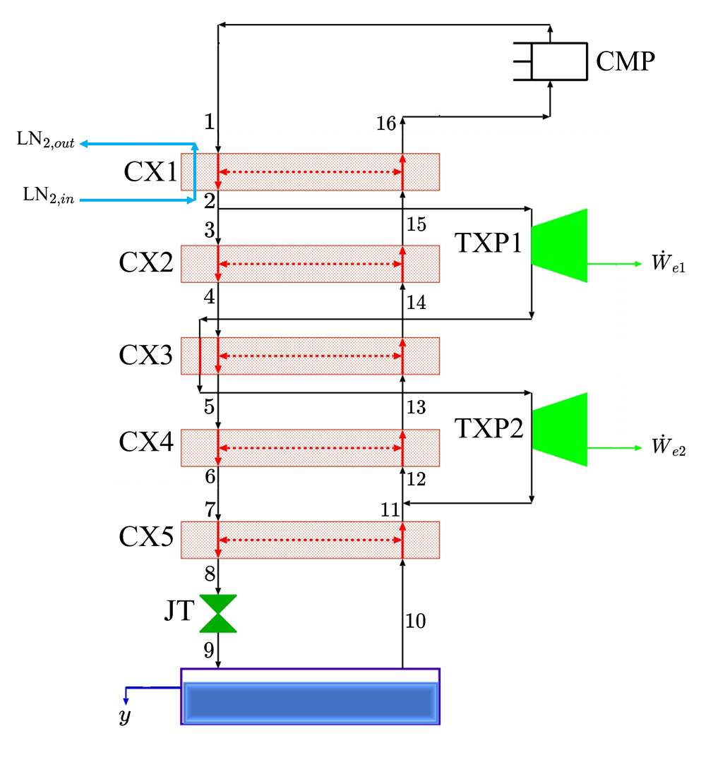
Figure 1: Schematics of the FREIA liquefier.

The warm gas (up to 42 g/s) leaves the compressor, labeled CMP, at about 13 bar and passes through five counterflow heat exchangers (CXn) in the left (warm) branch of the liquefier, before a Joule-Thomson valve (JT) expands it and cools it to about 4 K at 1.2 bar into the two-phase reservoir, shown at the bottom of Fig. 1, from which the liquid helium is extracted. The cold gas returns towards the compressor through the cold side of the five heat exchangers, such that it cools the gas on the warm side. A fraction of the gas is directed from the warm side at point 2 and passes through two turbo-expanders (TXPn) that expand the gas and thereby extract energy. The expanded gas after TXP1 passes near the warm side of CX3, which helps to cool the gas on the warm side, before TXP2 cools it further and returns the cold gas to the cold side at point 11. Finally, liquid nitrogen can be passed through a third branch of CX1, where it efficiently helps to cool the gas that arrives in the liquefier with ambient temperature.

2 Simulation

We simulate the liquefier with MATLAB [5], where we characterize the state of the gas at each point in the liquefier by the temperature $T$, the pressure $P$, and the gas flow $Q$. All other thermodynamics potentials, such as the enthalpy, are then calculated with CoolProp [6], which, as a matter of fact, can convert any two (intensive) thermodynamics quantities to all others, which we extensively use in our simulation. Moreover, real properties, such as heat capacities or specific enthalpies of real gases are treated in a consistent way. The action of CMP, CX, and TXP on the state can be represented by matrices. Only the JT-valve is a non-linear element, such that we determine the equilibrium condition of the system by finding a zero of a one-dimensional non-linear function (depending on the extracted liquid) that internally solves all the linear relations. This makes solving the system very fast. But before discussing the full system, we briefly address the actions of the different elements on the state.

3 Counterflow heat exchangers

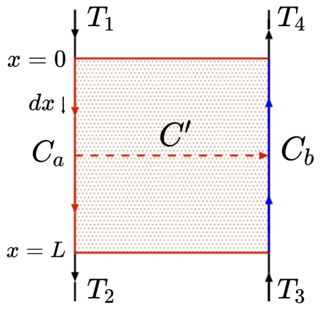
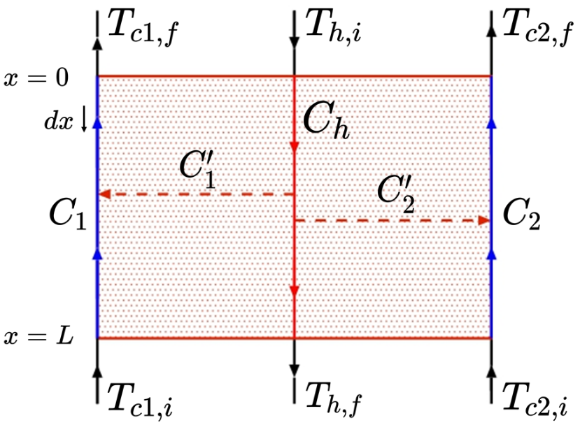
Figure 2: Two- (left) and three-way (right) heat exchanger.

The left side of Fig. 2 shows the two-way heat exchanger that we use for CX2, CX4, and CX5. The warm gas with temperature $T_{1}$ enters at the top left and leaves at the bottom left with $T_{2}$, whereas the cold gas enters enters from the bottom right with $T_{3}$ and leaves the heat exchanger at the top right with $T_{4}.$ From the enthalpy balance in a slice $dx$ of the warm and cold gas with heat capacities $C_{a}$ and $C_{b}$ and the heat exchanged with specific heat capacity (per meter) $C^{\prime}$, we find $d\dot{H}_{a}=-C_{a}dT_{a}$, $d\dot{H}_{b}=-C_{b}dT_{b}$, and $d\dot{H}=C^{\prime}(T_{a}-T_{b})dx$, where $\dot{H}$ is the enthalpy flow in the respective channels. Combining the equations leads to

$$\frac{dT_{a}}{dx}=-\frac{C^{\prime}}{C_{a}}(T_{a}-T_{b})\quad\mathrm{and}\quad\frac{dT_{b}}{dx}=-\frac{C^{\prime}}{C_{b}}(T_{a}-T_{b})\ ,$$ (1)

which are two coupled linear differential equations that are trivial to solve. Matching the boundary conditions to $T_{1},\dots,T_{4}$ then leads to the set of linear equations

$$T_{2}=T_{1}-\eta(T_{1}-T_{3})\quad\mathrm{and}\quad T_{4}=T_{3}+\eta\frac{C_{a}}{C_{b}}(T_{1}-T_{3})$$ (2)

where the efficiency $\eta$ is given [5] in terms of the heat capacities and the length $L$ of the heat exchanger. Integrating the enthalpy flow $d\dot{H}$ along $dx$, we find [5] the heat conduction constant $C_{H}$, which allows us to calculate the enthalpy flow from the warm to the cold side as $\Delta H=C_{H}(T_{1}-T_{3})$. In addition, $C^{\prime}$ can easily be generalized to three dimensions, as it is given by the product of the heat transfer coefficient and the contact area.

We treat the three-way heat exchangers CX1 and CX3 in much the same way, in our case with a hot flow (subscript $h$) and two cold flows (subscript $c$). Using the notation from the right-hand side in Fig. 2, we find the temperature change from the heat balance in a slice $dx$ to be

$$C^{\prime}_{1}dT_{c1}/dx=-C^{\prime}_{1}(T_{h}-T_{c1})$$ (3)

$$C_{2}dT_{c2}/dx=-C^{\prime}_{2}(T_{h}-T_{c2})$$ (4)

$$C_{h}dT_{h}/dx=-C^{\prime}_{1}(T_{h}-T_{c1})-C^{\prime}_{2}(T_{h}-T_{c2})$$ (5)

which is a linear system that can be solved analytically. As before, matching the boundary conditions gives us linear equations that relate the output temperatures $T_{c1,f},T_{c2,f},$ and $T_{h,f}$ to the input temperatures $T_{c1,i},T_{c2,i},$ and $T_{h,i}$. The details can be found in [5].

4 Turbo-expanders

A fraction $x$ of the mass flow $Q_{2}$ at point 2 is directed to the branch with the two turbo-expanders. We assume that they operate isentropically with $P_{in}/P_{out}=(V_{out}/V_{in})^{\gamma}$, where $\gamma=5/3$ for a monatomic ideal gas, and that the maximum speed is determined by the speed of sound at the respective temperatures, as supersonic velocities can reduce the turbo-expander efficiency. Following [7], together with the ideal gas law, this leads to the linear equations that relate the state variables of the output to the input variables: $T_{out}=T_{in}/2$ and $P_{out}=P_{in}/5.64.$

The mass flow through the branch with the two expanders is constant and returns to the cold return line at point 11, where we need to “mix” the gas flow $Q_{\textrm{TXP}}$ coming from the expanders and the gas coming from the reservoir. In order to satisfy the mass flow balance we have $Q_{12}=Q_{11}+Q_{\textrm{TXP}}$ and the enthalpy balance $Q_{12}h_{12}=Q_{11}h_{11}+Q_{\textrm{TXP}}h_{\textrm{TXP}}$, where we use CoolProp to determine the respective specific enthalpies.

5 Joule-Thomson valveand liquid extraction

Throttling the gas through a JT-valve between point 8 and 9 in Fig. 1 causes the pressure to drop from $P_{8}$ to $P_{9}$, which causes the temperature to drop in such a way that the enthalpy in the process remains constant. We model this process using CoolProp with the following code snippet

  h8=PropSI(’H’,’P’,P8,’T’,T8,’Helium’);
  h9=h8;
  T9=PropSI(’T’,’P’,P9,’H’,h9,’Helium’);

Here PropSI() is the MATLAB interface to the CoolProp library. The function receives two parameters and returns any other, here we supply the initial pressure $P_{8}$ and temperature $T_{8}$ to return the specific enthalpy $h_{8}$, which stays constant $h_{9}=h_{8}.$ In the second call, we calculate the temperature $T_{9}$ in the reservoir from the known reservoir pressure $P_{9}$ and the specific enthalpy $h_{9}.$

After using CoolProp to determine the specific enthalpies in the reservoir, $h_{\textrm{liq}}$ for the liquid and $h_{\textrm{gas}}$ for the gas, we obtain the extracted fraction $y$ from solving the enthalpy balance $h_{9}=yh_{\textrm{liq}}+(1-y)h_{\textrm{gas}}$ for $y$ and extract the fraction $y$ of the mass flow $Q_{9}$ from the gas $Q_{10}$ that returns through the cold side of the heat exchangers to the compressor.

6 Results

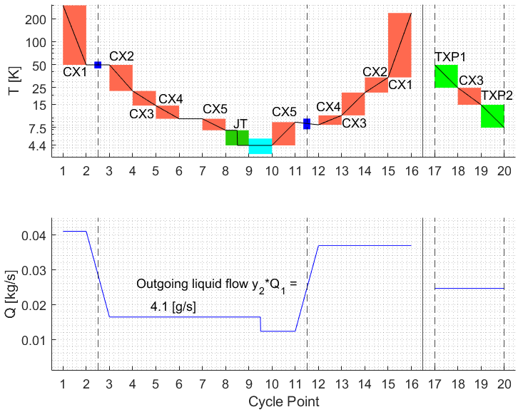
Figure 3: Performance with LN₂ pre-cooling.

After testing our simulation against textbook examples (Linde-Hampson, Claude, Collins) and carefully monitoring the balance of the mass flow and enthalpies at all stages, first without liquid nitrogen (LN₂) pre-cooling and then with LN₂ pre-cooling. The result of such a simulation is shown in Fig. 3. The horizontal axis labels the points that correspond to those indicated on Fig. 1 and on the upper panel we show the temperature at each point, with the effect of each heat exchanger CXn clearly indicated by the vertical size of the orange box that signifies the temperature change. The Joule-Thomson valve is indicated by a green box and the reservoir as a light blue box. Note also the dark blue dot between point 2 and 3, that shows the branch-off points of the mass flow through the turbo-expanders, separately shown on the far right of the plot between points 17 and 20, where point 17 corresponds to the blue dot between points 2 and 3. Point 20 links to the main branch between points 11 and 12, where the gas flows mix, as described above.

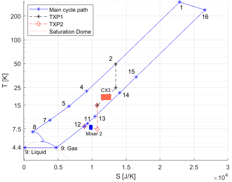
Figure 4: TS-diagram with LN₂ pre-cooling.

We also perform checks such that the enthalpy and gas flow are conserved over the simulated cycle. We then use CoolProp to calculate the entropy $S$ at each point in the cycle and show the temperature plotted versus the entropy in a $TS$-diagram in Fig. 4, where the numbers correspond to those in Figs. 1 and 3. This type of diagram is useful to visualize all the heat transfers in the whole cycle. Helium gas in the return flow from the cold box exits at point 16 close to ambient temperature and is heated up further in the piping back to the compressor at point 1. Point 1 to 8 and 9 to 16 respectively represent the isobaric cooling and heating of the gas through the heat exchangers. The separate turbo-expander flow is also visible. Point 8 to 9 describe the isenthalpic process in the JT valve, until the gas reaches the saturation dome (marked in Fig. 4) and follows the saturated vapour line, whereas some of the gas is left as liquid in the reservoir.

We adjust the model parameter values, such as the heat exchange design parameter $C^{\prime}$, to match the performance of the real liquefier. The simulated value of the yield over the whole cycle is found to be 6.1% without LN₂ pre-cooling and 10% with LN₂ pre-cooling, with compressor pressure $P_{1}=12$ bar(a) and reservoir pressure $P_{9}=1.12$ bar(a). The respective values for the yield in the real liquefier is 5-6% and 10%. Although temperature and gas sensors are not installed at all cycle points, the simulations show similar values where there are such sensors.

In order to find the theoretical maximum yield of the cycle, we vary the model parameters in different combinations. Changing the pressures $P_{1}$ and $P_{9}$ as well as the initial gas flow $Q_{1}$ down to 50% of their initial values has little impact on the yield $y$ in the simulations, a few percentage points at most. The maximum simulated yield of 17.6% is obtained by increasing the coupling $C_{1}^{\prime}$ (between the hot flow and the cold return flow) in CX1, decreasing the coupling $C_{2}^{\prime}$ with the LN₂ cooling in CX1, and slightly increasing the turbo-expander mass flow fraction $x$. Although the real heat exchangers have technical limitations in how much $C^{\prime}$ can be increased, these optimizations can indicate possible performance improvements for the liquefaction.

7 Conclusions

We developed a theoretical model of the helium liquefier in the FREIA Laboratory in MATLAB, starting from enthalpy conservation. The main objective was to find the unknown parameters not specified in the manual of the manufacturer. All the components in the thermodynamic cycle were represented by matrices, except the Joule-Thomson valve for which we used the CoolProp library for the non-linear mapping of the state variables. We observed simulated liquefaction yields similar to the real liquefier, with and without LN₂ pre-cooling. Adjusting model parameters allowed us to obtain higher yields and might indicate the promising points to improve the performance of the liquefier.

References

- [1] R. Ruber et al., Accelerator Development at the FREIA Laboratory, https://arxiv.org/abs/2103.05265
- [2] H. Li, et al., RF Performance of the spoke prototype cryomodule for ESS, FREIA Report 2019/08; http://uu.diva-portal.org/smash/record.jsf?pid=diva2%3A1427442.
- [3] A. Miyazaki et al., First cold test of a crab cavity at the GERSEMI cryostat for the HL-LHC project, http://uu.diva-portal.org/smash/record.jsf?pid=diva2%3A1501277
- [4] K. Pepitone, in preparation.
- [5] E. Waagaard, Benchmarking a cryogenic code for the FREIA helium liquefier, FREIA Report 2020/01; available from http://uu.diva-portal.org/smash/record.jsf?pid=diva2%3A1438754&dswid=4228.
- [6] I. Bell et al., Pure and Pseudo-pure Fluid Thermophysical Property Evaluation and the Open-Source Thermophysical Property Library CoolProp, Ind. Eng. Chem. Res. 52 (2014) 2498; and at http://www.coolprop.org
- [7] T. Flynn, Cryogenic engineering, CRC Press, Baton Roca, Fl., 2004.