Reflections on the photodissociation of CO in circumstellar envelopes

Carbon monoxide (CO) is the most abundant molecule after molecular hydrogen and is important for the chemistry in circumstellar envelopes around evolved stars. When modelling the strength and shape of molecular lines, the size of the CO envelope is an input parameter and influences the derived mass-loss rates. In particular the low-J transition CO lines are sensitive to the CO photodissociation radius. Recently, new CO photodissociation radii have been published using different formalisms that differ considerably. One set of calculations is based on an escape-probability formalisms that uses numerical approximations derived in the early-eighties. The accuracy of these approximations is investigated and it is shown that they are less accurate than claimed. Improved formalism are derived. Nevertheless, the changes in CO envelope size are small to moderate, less than 2% for models with $10^{-7}<\dot{M}<10^{-4}$ $M_{\odot}$ yr^-1 and at most 7% for model with $\dot{M}=10^{-8}$ $M_{\odot}$ yr^-1.

1 Introduction

Essentially all low- and intermediate mass stars end their lives on the asymptotic giant branch (AGB), where they loose their enveloppe (of order $\sim$0.5 to 6.5$M_{\odot}$ depending on inital mass) that is returned to the interstellar medium (ISM) in the form of dust and gas. Determining the mass-loss rate (MLR) is of key importance in understanding AGB evolution in detail. One of the main methods to do so is to use carbon monoxide (CO) as it is the most abundant molecule after molecular hydrogen and is very stable to photodissociation (see Höfner & Olofsson 2018 for an overview). As CO also essentially binds all carbon when C/O$<$1 (oxgygen-rich stars, or O-stars) and all oxygen when C/O$>$1 (carbon-rich stars, or C-stars) the molecule is also important for the chemistry in the circumstellar envelopes (CSEs) around AGB stars, see e.g. Agúndez et al. (2020).

When performing detailed radiative transfer modelling of CO-lines (typically fitting multiple transitions) to determine the MLR (see e.g. Sahai 1990; Groenewegen 1994; Schöier & Olofsson 2001; Decin et al. 2006) an CO abundance profile is required as input. The CO density is usually parameterised as

$$n_{\rm CO}\propto f_{\rm CO}\exp\left(-\ln(2)\left(\frac{r}{R_{\frac{1}{2}}}\right)^{\alpha}\right),$$ (1)

where $f_{\rm CO}$ is the photospheric CO abundance, $r$ is the distance to the star, $R_{\frac{1}{2}}$ the distance where the CO abundance is half the photospheric value (and typicaly called the photodissociation radius), and $\alpha$ describes the shape of the profile.

Recently, Groenewegen (2017) and Saberi et al. (2019) presented results of photodissociation calculations of CO (i.e. values for $R_{\frac{1}{2}}$ and $\alpha$) for a large grid of MLRs, expansion velocities, $f_{\rm CO}$ values, and strenghts of the interstellar radiation field (ISRF). Both papers were updates of Mamon et al. (1988) that was the classical reference for the CO photodissociation radii in circumstellar envelopes for almost thirty years. Both papers used different approaches and the CO photodissociation radii found by Saberi et al. (2019) are 11-60% smaller than found by Groenewegen (2017) (Saberi et al., 2019).

Groenewegen (2017) used the approach introduced in Li et al. (2014, 2016). It is based on the shielding functions of Visser et al. (2009), that depend on the column density of CO and molecular hydrogen (H₂), and a numerical integration scheme that takes into account the fact that at any point in the wind UV photons can arrive from all directions (see Appendices A in Li et al. 2014 and Groenewegen 2017). The shielding functions from Visser et al. (2009) were derived for a static environment however.

Saberi et al. (2019) have used the escape-probability formalism developed for an expanding envelope by Morris & Jura (1983) (herafter MJ83) and later updated by Mamon et al. (1988). They used the latest updated molecular data for CO from Visser et al. (2009) and for H₂ to calculate the CO shielding functions.

Both models assume spherical symmetry, a smooth wind (that is no clumps), a constant velocity in the outflow, and simplified scattering and absorption properties of the dust in the 912 – 1076 Å region.

In the escape-probability formalism the relevant integrations over angle are replaced by numerical approximations developed in MJ83. These approximations have been derived for a certain parameter space of line and continumm optical depths, but neither Mamon et al. (1988) and Saberi et al. (2019) checked whether these conditions are in fact met.

In this paper the validity of these approximations is investigated, and an improved formalism proposed.

The mathematical problem and numerical solution to this problem are presented in Sect. 2. The calculations are presented in Sect. 3 and discussed in Sect. 4, while Sect. 5 concludes this paper.

2 Equations and solutions

Two equations are relevant in the description of the photodissociation process of CO. The first is a term describing the continuum absorption of radiation,

$$\gamma=\frac{1}{2}\int_{0}^{\pi}d\phi\sin\phi\;\exp\left(-\tau_{\rm c}\;\phi/\sin\phi\right),$$ (2)

where $\phi$ is the angle with respect to the radius vector from the central star (MJ83) and its numerical approximation,

$$\gamma=\exp\left(-1.644\;\tau_{\rm c}^{0.86}\right)$$ (3)

‘with an accuracy of 1% for $\tau_{\rm c}<5$’ (Eq. 5 in MJ83), where $\tau_{\rm c}$ is the continuum optical depth measured radially outwards from a point at distance $r$ from the central star.

In MJ83 only the continuum absorption by dust was considered $(\tau_{\rm d})$ but also the contribution in the line wings of H₂ transitions $(\tau_{\rm H_{2}})$ should be included, $\tau_{\rm c}=\tau_{\rm d}+\tau_{\rm H_{2}}$ (see the discussion in Mamon et al. 1988 and Eq. A14 in Saberi et al. 2019).

The second relevant equation describes the escape probability for a line photon,

$$\beta = \frac{1}{2}\int_{0}^{\pi}d\phi\sin\phi\;\exp\left(-\tau_{\rm c}\;\phi/\sin\phi\right)$$ (4)

$$\cdot\left(1-\exp\left(-\tau_{\rm i}/\sin^{2}\phi\right)\right)/\left(\tau_{\rm i}/\sin^{2}\phi\right),$$

which is approximated as

$$\beta=\gamma\;[\left(1-\exp(-\alpha\;\tau_{\rm i})\right)/(\alpha\;\tau_{\rm i})-\Delta]$$ (5)

with $\alpha=1.5$, ‘where $\Delta$ is a small correction without which this expression for $\beta$ is accurate to within 10%’ (Eq. 8 in MJ83). When

$$\Delta=0.20\;\exp(-0.94\;\tau_{\rm i})\left(1-\exp(-\tau_{\rm i}^{1.45}/1.5)\right)/\tau_{\rm i},$$ (6)

Equation 5 ‘is accurate to $<0.5$% if $\tau_{\rm d}$ = 0 and a few percent when $\tau_{\rm d}\neq$ 0’ (Eq. 9 in MJ83). Again, the line optical depth $\tau_{\rm i}$ is measured outwards from a point in the envelope at distance $r$.

It should be pointed out that Mamon et al. (1988) and Saberi et al. (2019) ignore the $\Delta$ term (see the Appendix in Mamon et al. 1988 and Eq. A4 in Saberi et al. 2019). These two papers also used a different notation in the sense that the term between square brackets is denoted $\beta$ corresponding to the CO self-shielding and they labeled $\gamma$ for CO-mutual shielding by H₂ and dust.

It is remarked that Eqs. 2 and 4 ignore the finite size of the central star. Assuming that all radiation from behind the central star is blocked, and that the UV emission of the central star itself may be ignored, the integration over $\phi$ effectively runs from 0 to $(\pi-\beta),$ where

$$\sin\beta=\frac{R_{\star}}{r}$$ (7)

indicates the angle subtended by the central star (or the inner radius of the envelope) from a point at distance $r$ (see Eq. 5 and Fig. A1 in Groenewegen 2017). This effect was taken into account in Groenewegen (2017), while the approximations in MJ83 assume that the central star is a point source.

The results in the next section have been obtained using routines written in Fortran77 from Press et al. (1992): a Romberg integration schema (qromb) to perform the numerical integrations, and a nonlinear least-squares fitting routine (a Levenberg-Marquardt algorithm, mrqmin) to derive the coefficients in Eqs. 3, 5, and 6. The precision of the numerical integration routine has been verified by comparing selected results to those obtained using an on-line tool for such calculations.

3 Results

3.1 Calculation of $\gamma$

Figure 1 and Table 4 contain the results of the calculation of $\gamma$. The upper two panels illustrate the results for $\tau_{\rm c}<5$. Panel (a) show the exact calculation of $\gamma$ against $\tau_{\rm c}$. The approximation of Eq. 3 is also plotted, but they are indistinguishable. Panel (b) shows the ratio of the exact calculation to that approximation. The maximum deviation is $\approx 1.5\%$, larger than claimed in MJ83. One observes that in this range in optical depth the approximation is systematically lower (by $\approx 0.5\%$) than the exact calculation. For larger optical depths the deviations become increasingly larger, up to a factor of two at $\tau_{\rm c}\approx 16$ (Table 4).

As the numerical integration scheme is compared to a fitting formulae there is no observational error as such to be used in a classical $\chi^{2}$ analysis. Instead, an error will be assigned such that the final fitting formulae (Eqs. 11, 12) will have a reduced $\chi^{2}$ of unity. This will allow to monitor the reduced $\chi^{2}$ in the several fitting steps and will give representative error bars in the fitting coefficients.

Comparing in a chi-square sense Eq. 3 (with fixed coefficients $-1.644$ and $0.86$) to the exact calculations over the range $0<\tau_{\rm c}<5$ in steps of 0.025 units will result in a reduced $\chi^{2}$ of 7.3 if an ‘error’ of 0.35% (see below) is assigned to each data point. Fitting for the coefficients and finding the solution with the smallest maximum deviation over the largest possible range in $\tau_{\rm c}$ results in the best fit of:

$$\gamma=\exp\left((-1.6375\pm 0.0003)\;\tau_{\rm c}^{(0.8618\pm 0.0002)}\right),$$ (8)

made in the range $\tau_{\rm c}<5.3$. The maximum deviations are $\pm 1.2\%$ and the reduced $\chi^{2}$ becomes 2.0, a significant reduction, indicating that the fit is much improved although the coefficients are similar. Panel (c) is a repeat of panel (b) for this approximation showing that the deviations are now more symmetric around unity.

Table 1: Calculations for $\gamma$.

$\tau_{\rm c}$	$\gamma$	exact/approx.	exact/approx3.
	(exact)	Eq. 3	Eq. 8
0.050	0.8938	1.013	1.012
0.075	0.8486	1.013	1.012
0.650	0.3215	1.000	0.995
0.725	0.2874	1.000	0.994
0.850	0.2393	1.000	0.994
0.975	0.2001	1.000	0.993
3.325	0.0010	1.015	1.006
5.000	0.00142	1.001	0.994
5.300	0.00101	0.996	0.989
7.050	0.00014	0.950	0.946
8.375	0.00003	0.900	0.899
10.55	3.1 (-6)	0.800	0.802
12.48	3.9 (-7)	0.700	0.705
14.35	5.3 (-8)	0.600	0.609
16.35	6.4 (-9)	0.500	0.509

Figure 1: Natural logarithm of $\gamma$ plotted against continuum optical depth (panel a), with the ratio of the exact solution to the approximation in MJ83, Eq. 3, in (panel b). Panel (c) show this ratio for the new best fit, Eq. 8.

3.2 Calculation of $\beta$

Figure 2 compares the exact numerical results for the calculation of ($\beta/\gamma$) in the range $\tau_{\rm i}<5$ and $\tau_{\rm c}<5$, to the approximation in Eq. 5 with $\Delta=0$ and $\gamma$ approximated by Eq. 3. The differences are much larger than the claimed 10%, almost 25% near $\tau_{\rm i}=2.5$ (and for $\tau_{\rm c}=5$). Deviations of less than 10% are only reached in a very limited range of $\tau_{\rm i}$ and $\tau_{\rm c}$. Technically speaking, the claimed accuracies are on $\beta$, while $\beta/\gamma$ is considered here, but as approximation Eq. 5 is accurate to about 1.5% this has little practical effect. The deviations from unity appear to reach a constant level for large $\tau_{\rm i}$ and also depend on $\tau_{\rm c}$. The top panels in Fig. 3 highlights this by showing the results for $\tau_{\rm i}<15$ and the restricted range $\tau_{\rm c}<2.5$. At large optical depths the deviations are at most 10%, but at $\tau_{\rm i}\sim 1.5$ it is 15%.

The minimum in the ratio of exact-to-approximation curve near $\tau_{\rm i}\sim 1$ can be largely removed by including the term $\Delta$, as shown in the bottom panels Fig. 3. It shows the results for $\tau_{\rm i}<5$, $\tau_{\rm c}<2.5$, and using Eq. 6 for $\Delta$. The deviations from unity are now quite uniform with $\tau_{\rm i}$.

Taking the calculations with limits $\tau_{\rm i}<5$, $\tau_{\rm c}<2.5$ and the approximations Eq. 3, and Eq. 5 with $\Delta=0$ as reference (the default in Mamon et al. (1988) and Saberi et al. (2019)), the reduced $\chi^{2}$ is 45 when assigning an ‘error’ of 1.0% per datapoint (see below) in $\beta/\gamma$. Performing a fit in the range $\tau_{\rm i}<15$, $\tau_{\rm c}<2.5$ and the better approximation Eq. 8 for $\gamma$, the best fit is Eq. 5 with $\alpha=1.5222\pm 0.0001$ and

$$\Delta = (0.154\pm 0.006)\;\exp(-(0.852\pm 0.015)\;\tau_{\rm i})$$ (9)

$$\cdot\left(1-\exp(-(0.92\pm 0.04)\;\tau_{\rm i}^{(1.441\pm 0.006)})\right)/\tau_{\rm i},$$

with a reduced $\chi^{2}$ of 25. This fit is shown in Fig. 4.

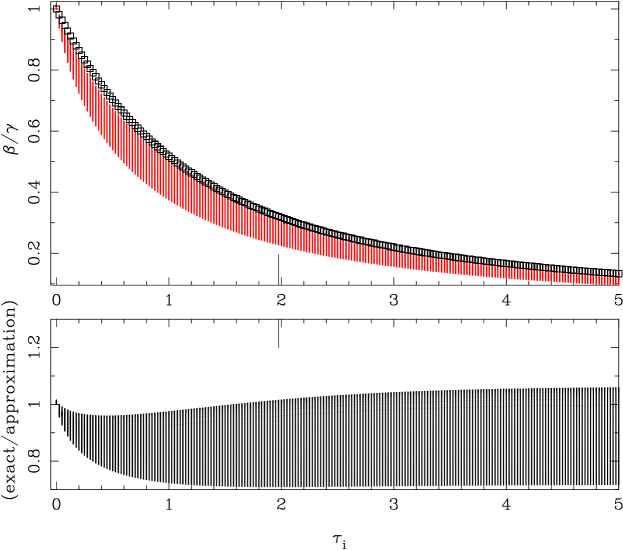
Figure 2: Ratio of $\beta$ over $\gamma$ plotted against line optical depth, for the approximation in MJ83: Eq. 3 and Eq. 5 with $\alpha=1.5$ and $\Delta=0$ and calculated for $\tau_{\rm c}<5$. The approximation is plotted with small squares in the upper panel. The ratio of the exact solution to the assumed approximation is shown in the bottom panel. For each discrete value of $\tau_{\rm i}$ (calculated at 0.025 intervals) the vertical lines indicate the range in continuum optical depth, from 0 (largest value of $\beta$/$\gamma$) to the maximum value (lowest value). The small vertical lines at the bottom of the upper and at the top of the bottom panel indicate the optical depth where the difference between the exact calculation and the approximation is largest.

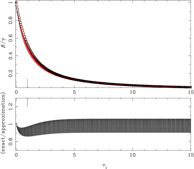
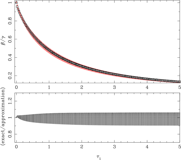
Figure 3: As Fig. 2, but with $\tau_{\rm c}$ limited to $<2.5$ (the top two panels). The calculations in the bottom two panels show the results with the $\Delta$ term included (Eq. 6). that make the ratio of exact calculation to approximation more symmetric around unity.

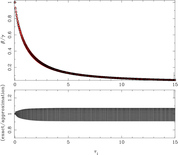
Figure 4: As Fig. 2 for $\tau_{\rm c}<2.5$ using the new best fit: Eq. 8, Eq. 5 with $\alpha=1.522$ and Eq. 9.

4 Average escape probabilities

In the previous section we showed that the approximations in MJ83 have limitations, but it is not clear how this might affect a full calculation including all CO lines which cover a large range in optical depths.

To investigate this further, we considered the optical depths of the 855 CO lines for the standard model in Saberi et al. (2019), with parameters MLR $\dot{M}$= 10^-5 $M_{\odot}$ yr^-1, wind expansion velocity $V_{\rm exp}=$ 15 km s^-1, $f_{\rm CO}$= 8 $\cdot 10^{-4}$, at a distance of $r=10^{16}$ cm, which implies a kinetic temperature of $\sim 70$ K (from Eq. 1 in Saberi et al. 2019). The CO line optical depth $\tau_{\rm i}$ ranges from 0.25 to $\sim 900$ with a median of 35. The continuum optical depth $\tau_{\rm H_{2}}$ in the line wings of H₂ lines at the wavelengths of the CO lines ranges from 0.12 to $>$10 000 with a median of 1.3. The dust optical depth $\tau_{\rm d}$ is 4.14.

These optical depths scale like $\sim$ $\dot{M}$$f_{\rm CO}$/ $V_{\rm exp}$ /$r$. Groenewegen (2017) and Saberi et al. (2019) considered MLRs from 10^-4-10^-8 $M_{\odot}$ yr^-1, expansion velocities from 3.75-30 km s^-1, and CO abundances from 2-16 $\cdot 10^{-4}$. The range in distances is taken from where the abundance (cf. Eq. 1) changes from (0.999 $\cdot$ $f_{\rm CO}$) to (2 $\cdot$ $R_{\frac{1}{2}}$). Using the approximations in Groenewegen (2017) for $R_{\frac{1}{2}}$ and $\alpha$ as a function of MLR, $f_{\rm CO}$, and $V_{\rm exp}$ it is determined that the optical depths range from about unity to $10^{-4}$ times those of the standard case considering the entire parameter space.

Table 5 summarises the calculations for the average escape probability

$$\overline{\beta}=\sum_{i=1}^{855}\;\beta_{i}$$ (10)

over all CO lines for different scaling factors of the optical depth. The escape probability is calculated: a) exactly, b) using the approximations in MGH and Saberi et al. 2019 (Eq. 3 and Eq. 5 with $\alpha=1.5$ and $\Delta=0$), and c) the improved approximations (Eq. 5 with $\alpha=1.522$ and Eq. 9), in Cols. 2, 3, and 4 respectively.

For the standard model the improved approximation is closer to the exact calculation, but still off by about 30%. In the standard model scaled downwards one observes the trend that the simple approximation systematically gives too large average escape probabilities, while the improved approximation systematically gives lower values than the exact calculation. The simple approximation actually gives results closer to the exact calculation, which is surprising in view of the results presented in Sects. 3.1 and 3.2.

A closer inspection of the optical depths shows that in the standard case in 769 of the 855 lines $\tau_{\rm i}>15$ or $\tau_{\rm c}>5$ (and both conditions are violated in 365 lines), that is, values for the optical depths outside the range of the fitting formula.

Considering the optical depth of all 855 lines for the 5 sets of models, and choosing escape probabilities of $>$ 0.001 as being the most relevant, we find that in 90% of the cases the optical depths are $\tau_{\rm i}<7$ and $\tau_{\rm c}<1$. This indicates that the line and continuum optical depths in realistic cases covers a more restricted range than considered in MJ83 and earlier in this paper. Given this finding the fits to $\gamma$ and $\beta/\gamma$ were repeated using these limits, and the results are

$$\gamma=\exp\left((-1.6488\pm 0.0013)\;\tau_{\rm c}^{(0.8724\pm 0.0015)}\right),$$ (11)

a value of $\alpha=1.4376\pm 0.0006$ in Eq. 5, and

$$\Delta = (0.12\pm 0.01)\;\exp(-(0.75\pm 0.04)\;\tau_{\rm i})$$ (12)

$$\cdot\left(1-\exp(-(1.00\pm 0.09)\;\tau_{\rm i}^{(1.47\pm 0.01)})\right)/\tau_{\rm i}.$$

By earlier choosing the error per datapoint as 0.35% and 1.0%, respectively, the reduced $\chi^{2}$s are tuned to be unity in both fits. With this new approximation the average escape probabilities (the last column in Table 5) are very close to the exact values, except in the standard case, where the functional forms of Eqs. 3 and 5 do not provide an adequate description.

Table 2: Average escape probability calculated under different assumptions.

Standard model	$\overline{\beta}$	$\overline{\beta}$	$\overline{\beta}$	$\overline{\beta}$
$\cdot$ 1	4.22 (-5)	5.73 (-5)	5.56 (-5)	5.04 (-5)
$\cdot$ 0.1	8.18 (-2)	8.35 (-2)	7.84 (-2)	8.16 (-2)
$\cdot$ 0.01	0.492	0.507	0.478	0.491
$\cdot$ 0.001	0.840	0.859	0.827	0.838
$\cdot$ 0.0001	0.963	0.969	0.954	0.959

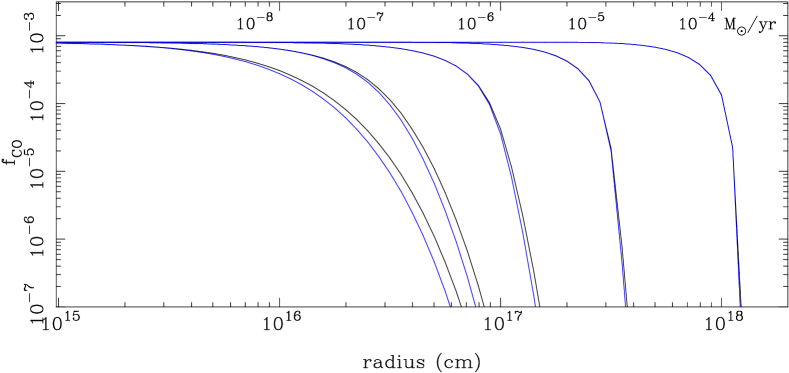
Figure 5: CO abundance profile for the 5 indicated MLRs. Blue lines indicate the profiles using the approximations used in Saberi et al. (2019), black lines indicate the profiles using the improved approximations.

5 Summary and discussion

Improved numerical approximations are outlined to the formalism presented in MJ83 and that are at the basis of the CO photodissociation calculations in Mamon et al. (1988) and Saberi et al. (2019). The results in Table 5 show that the average escape probability in realistic cases deviate by 2-3% from the exact value for low to moderate MLRs (and 35% for large MLRs) in the approximation used by Mamon et al. (1988) and Saberi et al. (2019), and $\stackrel{{\scriptstyle<}}{{\sim}}$0.4% (19%) in the improved approximation. For the quantity ($1-\overline{\beta}$) the differences are 0.002 - 19%, respectively, 0.001 - 11%, with the largest difference for the smallest MLRs.

The improved approximations were implemented in the code used in Saberi et al. (2019) and some calculations were performed using $V_{\rm exp}=$ 15 km s^-1, $f_{\rm CO}$= 8 $\cdot 10^{-4}$, and MLRs $\dot{M}$= 10^-4, 10^-5, 10^-6, 10^-7, 10^-8 $M_{\odot}$ yr^-1. Figure 5 shows the CO abundance versus distance to the star for the 5 MLRs, from which $R_{\frac{1}{2}}$ is determined. The improved formulae lead to a larger photodissociation radius by 7.2% for $\dot{M}$= 10^-8, 2.2% for 10^-7 $M_{\odot}$ yr^-1, and $\stackrel{{\scriptstyle<}}{{\sim}}$0.5% difference for the other MLRs. A larger photodissociation radius is expected as the escape probability is lower in the improved approximation compared to the classical approximation.

As basic assumptions of spherical symmetry, constant velocity, and smooth outflow are identical in the Groenewegen (2017) and Saberi et al. (2019) models (see the introduction) the differences in the CO photodissociation radii (11-60% smaller in Saberi et al. (2019) than Groenewegen (2017)) can not be attributed to them. These differences are due to the different underlying physical implementation, the CO shielding function derived for a static environment (not representative of an AGB wind), and the escape-probability formalism in an expanding envelope, respectively. It is shown here that the numerical approximations used in the latter formalism have a small effect on the outcome.

The model by Saberi et al. (2019) is currently the most accurate avialable and covers a large parameter space (in MLR, $V_{\rm exp}$, $f_{\rm CO}$, ISRF strength). The results in the present paper show that the CO photodissociation radii are underestimated by a few percent for the lowest MLRs in Saberi et al. (2019), but uncertainties in observational estimates of MLR and $f_{\rm CO}$ lead to larger uncertainties.

Resolved observations of CO shells, like those carried out within the DEATHSTAR project (Ramstedt et al., 2020) will allow for a detailed comparison of predicted and observed CO photodissociation radii for a large sample in the near future.