Tackling Variabilities in Autonomous Driving

Abstract

The state-of-the-art driving automation system demands extreme computational resources to meet rigorous accuracy and latency requirements. Though emerging driving automation computing platforms are based on ASIC to provide better performance and power guarantee, building such an accelerator-based computing platform for driving automation still present challenges. First, the workloads mix and performance requirements exposed to driving automation system present significant variability. Second, with more cameras/sensors integrated in a future fully autonomous driving vehicle, a heterogeneous multi-accelerator architecture substrate is needed that requires a design space exploration for a new form of parallelism. In this work, we aim to extensively explore the above system design challenges and these challenges motivate us to propose a comprehensive framework that synergistically handles the heterogeneous hardware accelerator design principles, system design criteria, and task scheduling mechanism. Specifically, we propose a novel heterogeneous multi-core AI accelerator (HMAI) to provide the hardware substrate for the driving automation tasks with variability. We also define system design criteria to better utilize hardware resources and achieve increased throughput while satisfying the performance and energy restrictions. Finally, we propose a deep reinforcement learning (RL)-based task scheduling mechanism FlexAI, to resolve task mapping issue. Experimental results show that with FlexAI scheduling, basically 100% tasks in each driving route can be processed by HMAI within their required period to ensure safety, and FlexAI can also maximally reduce the breaking distance up to 96% as compared to typical heuristics and guided random-search-based algorithms.

1 Introduction

The state-of-the-art driving automation system demands extreme computational resources to meet rigorous accuracy and latency requirements. The traditional single accelerator-based on-car computer system, such as Mobileye EyeQ3 [1], and integrated GPU based platform, such as Nvidia Drive PX2, have shown staggering performance and limited processing capability when facing this performance demands  [2]. Therefore, emerging driving automation computing platforms such as Tesla FSD [3] and Horizon Journey 2 [4] propose ASIC-based computing platform that targets explicitly to neural-network-based task processing with regards to both performance and energy considerations. However, building such an accelerator-based computing platform for driving automation present following challenges.

First, the workloads mix and performance requirements exposed to driving automation system present significant variability. For example, an automated driving vehicle usually operates a variety of concurrent neural network (NN)-based tasks, such as visual perception-based assistant driving (e.g., object detection and recognition, scene segmentation) [5], high-level route planning (e.g. localization based on HD map) [6], HD map crowdsourcing [7], and intelligent human-machine interaction(e.g., voice recognition, gesture recognition, and driver eye-tracking). Furthermore, an automated vehicle typically equips multiple cameras and sensors where different cameras (e.g., forward-facing or side-facing) have differentiated stream generation rates and accuracy requirements under different driving areas (e.g., urban, undivided-highway or highway) and different driving behaviors (e.g., going straight, turning or reversing). Such variability shown in performance requirements and workload mix significantly challenges the performance guarantee and complicates the design of underlying computing platform in driving automation system.

Second, with the increasing number of cameras and camera frame rate in automated vehicles, driving automation system will generate enormous data for real-time analysis (e.g., 1200 frames per second (FPS)). Unfortunately, most single accelerator-based platforms cannot meet this overwhelming processing requirements. For example, ADM-7V3 FPGA[8] only supports 314.2 FPS and Virtex-7 VC707[9] only supports 109.3 FPS. With more cameras/sensors integrated in a future fully autonomous driving vehicle (L5) and increasing frame rate of cameras [10], a multiple accelerator-based computing platform is desired. Considering the composite workload mix often involves running multiple NN models with distinct layer operations and sizes, this will call for a heterogeneous multi-accelerator architecture substrate that requires a design space exploration for a new form of parallelism. As advocated in  [11], the performance or efficiency of future computer systems will have to rely on new accelerator-level parallelism (ALP). A high ALP implies that each accelerator can execute a targeted computation class faster and usually with less energy.

These observations prompt us to consider an important question: how can a driving automation computing system well-manage these challenging design aspects under rigorous performance and energy restrictions? To wit, to efficiently process such a large amount of CNN-based tasks with high variability on the complicated heterogeneous hardware substrate, effective criteria for system design that are tailored to driving automation should be defined, and efficient task scheduling mechanism should be explored to meet the criteria. Unfortunately, current computing systems for driving automation have not provided answers to this question.

In this work, we aim to extensively explore the above system design challenges and build a comprehensive driving automation framework that synergistically handles the key design aspects. First, our framework features a novel heterogeneous multi-core AI accelerator (HMAI) to provide the hardware substrate for the driving automation tasks with variability. We also propose the design principle to choose the accelerators for the HMAI. Second, our framework defines system design criteria to better utilize hardware resources and achieve increased throughput while satisfying the performance and energy restrictions. Specifically, we propose two metrics, Matching Score (MS) and Global State Value (Gvalue) to formalize the criteria. MS pays attention to the safety requirements of various tasks in driving automation systems, while Gvalue puts more weight onto the overall performance of HMAI that reflects the globality. Finally, our framework employs a deep reinforcement learning (RL)-based task scheduling mechanism FlexAI, to resolve the task mapping issue. Specifically, we show that a robust policy can be yielded by applying deep Q-network (DQN)[12]. The RL agent in FlexAI is predictive and global. The predictive means each policy will schedule a corresponding task immediately without considering the later-coming tasks. The global feature in FlexAI means it can consider the whole performance in hardware, such as resource utilization.

In an autonomous driving system, each task should be processed within a certain period to ensure driving safety. For instance, if a static obstacle cannot be detected by a moving vehicle within a specified period, it may cause a traffic accident. In this paper, with FlexAI scheduling, basically 100% tasks in each driving route can be processed by HMAI within their required period to ensure safety, while typical heuristics (e.g Min-Min), and guided random-search-based algorithms (GA, SA) can only ensure 21%, 34% and 51% safety on average, respectively. Moreover, FlexAI can maximally reduce the breaking distance up to 96% as compared to the above algorithms, thus efficiently avoiding traffic collision (traffic collision cause 36,096 people died in the United States in 2019 [13]). In addition, our experimental results also show that FlexAI achieves up to 87% execution time reduction and 960% resource utilization balance rate (introduced in Section 6.2) improvement, outperforming typical heuristics, guided random-search-based algorithms, and unscheduled algorithms. Moreover, HMAI can achieve up to 5× speedup and 2.5× TOPS/W over NVIDIA Tesla T4 GPU, and 2.1× TOPS/W over homogeneous hardware platforms (detail in Section 3.1).

2 Variabilities in Driving Automation

In this section, we show that the workload mix and performance requirements caused by the scenario change in driving automation are highly variable.

2.1 Heterogeneous CNN Models are Needed for Driving Automation Processing

The perception of an automated vehicle consists of a variety of workloads such as object detection (DET), object tracking (TRA), and localization (LOC) along the camera-to-recognition path. These diverse workloads can incur complex processing patterns to the underlying multi-accelerators. According to[14], DET, TRA, and LOC dominate the computing of the driving automation system. While for DET and TRA, the convolutional neural network (CNN)-based computation accounts for more than 94% of the execution time. Moreover, the DET and TRA are completely based on CNN-based camera data processing in Tesla[15], and even the LIDAR-based DET algorithms are mostly based on CNN[16]. Therefore, we will focus on CNN-based tasks in the driving automation system. Specifically, based on the research[14], we will focus on three typical CNN algorithms, the YOLO[17] and SSD[18] for DET, and GOTURN[19] for TRA. As shown in Table 1, we compare the key features of these three CNN algorithms.

CNNs	$\sharp$of MACs	$\sharp$of weights and neurons	Layers num
SSD	26G	697.76 M	53
YOLO	16G	150M	101
GOTURN	11G	13.95M	11

Table 1: The features of typical CNN algorithms in DET and TRA.

Object	Distance	Area	Proportion
Vehicle	163m	4620	0.33%
	17.98m	42000	3%
Pedestrian	140m	4620	0.33%
	15.48m	42000	3%

Table 2: The area and proportion of the objects in the image when they are at different distances from the current vehicle.

Method	Backbone	$AP_{S}$	$AP_{M}$	$AP_{L}$
YOLOv2[17]	DarkNet-53	18.3	35.4	41.9
SSD312[18]	ResNet-101	6.2	28.3	49.3
SSD512*[20]	VGG-16	10.9	31.8	43.5
SSD513[18]	ResNet-101	10.2	34.5	49.8

Table 3: Detection results of YOLO and SSD. $AP_{S}$ is AP of small objects, $AP_{M}$ is AP of medium objects and $AP_{L}$ is AP of large objects.

In this paper, we consider a co-run of multiple heterogeneous CNN-based perception models on a driving automation computing platform. This is motivated by the fact that driving automation scenarios present a diverse set of objects with different sizes, areas, and dynamic distances, which incur stringent and time-varying performance restrictions to the computing tasks. Take the representative driving automation data set KITTI[21] as an example. We show how the area of the representative object (vehicle and pedestrian) and its ratio to the area of entire image change with different distances in Table 2. Here the area is measured as the number of pixels in the segmentation mask. The small, medium, and large objects are defined as $(area<32^{2})$, $(32^{2}<area<96^{2})$ and $(area>96^{2})$. Considering the area of most images is $640\times 480$, the areas of small, medium, and large objects in each image account for 0.33%, 0.33%$\sim$3%, and 3% of the entire image area[22]. Notice that when the object vehicle is 17.98 meters away, it will be processed as a large object (i.e., 42000 pixels and account for 3% of the entire image). While when the object is 163 meters away, it will be processed as a small object. Similar observation also applies to pedestrian detection. Considering the vision of cameras ranges from 20 meters to 200 meters[23, 24], the captured image will include objects with various areas.

Facing such complicated workloads, a single CNN model struggles to meet the requirements of accuracy and detection time when the ranges of sizes and areas of objects are wide.   Tapping into heterogeneous CNNs is promising viability to mitigate this challenge. As shown in Table 3, YOLO and SSD show various achieved Average Precisions (AP) for different object areas. We can observe that YOLO is good at small and medium object detection, while SSD is good at large object detection. Therefore, the object detection tasks in automated vehicles demand heterogeneous CNN models to ensure accuracy.

2.2 Variability of Performance Requirements in Driving Automation Tasks

Driving automation is a highly safety-critical application. Its safety guarantee relies on rich surrounding information collected by its intensively integrated cameras and sensors. Up until 2018, the number of cameras in Tesla is 8, while Audi, BMW and Mercedes Benz use 5 cameras[25]. Uber’s self-driving Volvo SUV includes 7 cameras, and Ford Fusion includes 20 cameras to improve safety[26]. In March 2020, Waymo unveiled its fifth-generation self-driving system[27], which includes 29 cameras. According to this trend, it is reasonable to project that automated vehicles will deploy more than 30 cameras in the near future.

However, these cameras can generate video streams at various image rates ranging from 10 to 40 frame-per-second (FPS) depending on its function [6], and this will incur differentiated performance requirements for the backend hardware accelerators. We will show this challenge using an example. As shown in Table 4, we have 30 cameras which are configured into different function groups based on the configuration in Tesla, namely forward (FC), forward left side (FLSC), rearward left side (RLSC), forward right side (FRSC), rearward right side (RRSC) and rear cameras (RC). Figure 1 shows the required frame rates for each camera group under different driving areas, namely urban areas (UB), undivided-highway areas (UHW), and high-way areas (HW), and different driving scenarios, namely going straight (GS), turning left/right (TL), and reversing (RE). Notice that since reversing is not allowed on the highway, the corresponding frame rate of RC in HW is not provided.

Function	FC	FLSC	RLSC	FRSC	RRSC	RC
Camera number	11	4	4	4	4	3

Table 4: Configuration of cameras with different functions.

	DET	TRA	YOLO	SSD	GOTURN
Go straight(FPS)	870	840	435	435	840
Turn left(FPS)	950	920	475	475	920
Reverse(FPS)	740	740	370	370	740

Table 5: The performance requirements of vehicles in urban area. The requirement of turning right is same as turning left.

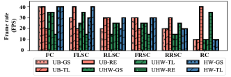
Figure 1: Frame rate requirements for different areas and scenarios.

Then, we can infer the requirements of image processing capability for each perception task in different areas. For example, Table 5 shows the FPS requirements for YOLO, SSD, and GOTURN in urban area under three driving scenarios. In going straight scenario, since object detection (DET) should be executed for all images from the cameras, the performance requirement is 870 FPS for the backend accelerator. However, since the object tracking is not supposed to perform for the rear cameras, the total performance requirement for object tracking (TRA) is 840 FPS. For the DET task, we use YOLO for small and medium object detection and use SSD for large object detection, hence the average processing capability for YOLO and SSD is 435 FPS. We use GOTURN to process the TRA task and the processing capability is 840 FPS.

We can observe that when the driving area or driving scenario changes, the FPS requirement for each camera in a vehicle will change consequently. Therefore, the amount of mixed CNN models that a vehicle needs to process within a certain period also will change accordingly.  Such variability in performance requirements and workload mix should be carefully handled by computing platform.

3 Design Challenges of Driving Automation System

Both industry[24, 23, 27] and academia[28, 29, 30, 31] are intensively exploring the driving automation system.The Society of Automobile Engineers (SAE)[32] defines six levels of driving automation from Level 0 to Level 5, where Level 5 is fully autonomous. To deliver a functional and practical driving automation system with a safety and reliability guarantee, designers should carefully analyze and optimize every technical detail from hardware through software. In this section, we explore the system design challenges imposed by the variability of workloads and performance requirements in driving automation. These challenges motivate us to propose a comprehensive framework that synergistically handles the heterogeneous hardware accelerator design principles, system design criteria, and task scheduling mechanism.

3.1 Hardware Platform Design

Multi-accelerator is Needed for Driving Automation Processing. The cameras and sensors on automated vehicles can generate a massive amount of data for real-time analysis. We show the relationship between the speed of the car and the requirements of the frame rates in Table 6, which are collected from multiple studies. We can observe that the required frame rate is around 20 FPS (frames per second). Note that a high frame rate is necessary for high-speed driving[33]. In KITTI the max frame rate for a speed of 90km/h could be 100 FPS. In industry practice, Audi sets the camera frame rate in driver assistance systems as 25 FPS [34]. The Tesla Model 3 adopts 36 FPS[35]. With the much higher safety requirements in the fully driving automation, the camera frame rates will be greater than 40 FPS in the future.

	Max velocity(km/h)	Frame rate(FPS)
KITTI[36]	90	10-100
ApolloScape[37]	30	30
Princeton[38]	80	10
VisLab[39]	70.9	>25
Oxford RobotCar[40]	Not Mentioned	11.1-16
Comma.ai[41]	Not Mentioned	20

Table 6: The camera frame rates in different researches.

Device type	YOLO type	Frame rate(FPS)
GTX TitanX[17]	Sim-YOLO-v2	88
GTX TitanX[42]	FAST YOLO	155
Zynq UltraScale+[43]	Tincy YOLO	30
Zynq UltraScale+[44]	Lightweight YOLO-v2	40.81
Virtex-7 VC707[9]	Tiny YOLO-v2	66.56
Virtex-7 VC707[9]	Sim-YOLO-v2	109.3
$ADM-7V3FPGA_{1}$[8]	Tiny YOLO	208.2
$ADM-7V3FPGA_{2}$[8]	Tiny YOLO	314.2

Table 7: Peak frame rates when run ML models on single accelerator.

	SconvOD (FPS)	SconvIC (FPS)	MconvMC (FPS)
YOLO	170.37	132.54	149.32
SSD	74.99	82.94	82.57
GOTURN	352.69	350.34	500.54

Table 8: The performance of various accelerators.

	YOLO	SSD	GOTURN
Go straight	(1 SO, 2 SI)	(3 SO, 1 SI, 2 MM)	(1 SI, 1 MM)
Turn left	(2 SO, 1 MM)	(2 SO, 4 SI)	(2 MM)
Reverse	(3 SI)	(2 SO, 3 MM)	(2 SO, 1 SI)

Table 9: The task allocation in (4 SconvOD, 4 SconvIC, 3 MconvMC). SO, SI and MM means SconvOD, SconvIC and MconvMC respectively.

With multiple cameras and high frame rate generation for each camera, a single automated car can generate enormous data and overwhelm the processing capability of a single accelerator. We quantify the capability of emerging accelerators in terms of peak frame rates, as shown in Table 7. We run the state-of-the-art object detection application YOLO and its derivations[17] on single accelerators. Note that though for some accelerators, the peak FPS can reach 314.2, it still cannot meet the maximum processing requirements of 1200 FPS. This is calculated based on the assumption of a car with 30 cameras and a generation rate of 40 FPS for each camera. Considering that Tesla FSD[3] has integrated four accelerators that can process 2300 frames per second, we can expect that future computing platforms for the automation system will base on multi-accelerator architecture.

Heterogeneous hardware is Needed for Driving Automation Processing. Here, we design three representative CNN accelerators (SconvOD, SconvIC, and MconvMC) based on our CNN accelerator taxonomy (detail in Section 5.1). By using these CNN accelerators, we can construct different homogeneous and heterogeneous platforms to process dynamic performance requirements in an autonomous driving system.

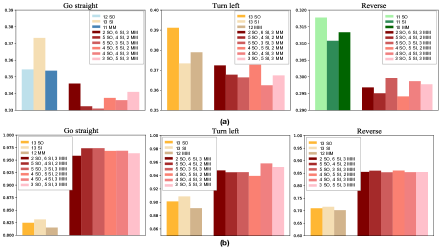
Figure 2: Comparison of (a) energy consumption and (b) resource utilization rate between homogeneous and heterogeneous platforms. SO, SI and MM means SconvOD, SconvIC and MconvMC, respectively.

For homogeneous platforms, according to the performance given in Table 8, we can obtain the number of accelerators required by each homogeneous platforms in different environments. Now, we will discuss the best configuration of each homogeneous platform under an assumption that a vehicle only travels in urban areas. When a vehicle is going straight, in order to meet the performance requirements in Table 5, for a homogeneous platform based on SconvOD, 3 SconvOD, 6 SconvOD, and 3 SconvOD are needed to process YOLO, SSD and GOTURN respectively, thus this homogeneous platform must contain 12 SconvOD. In the legend of Figure 2 (a), the most suitable accelerator number of each homogeneous platform in different scenarios are given. Figure 2 (a) shows the energy consumption of each homogeneous platform.

Since the hardware platform in the vehicle is fixed in advance, it needs to meet the performance requirements of all scenarios. For the homogeneous platforms based on the same accelerator in Figure 2 (a), we will choose the maximum number of accelerators in all scenarios to construct the final homogeneous platform. For instance, if the homogeneous platform is composed of SconvOD, the final platform will include 13 SconvOD. In Figure 2 (b), we show the resource utilization rate of different final homogeneous platforms in all scenarios.

When the heterogeneous platform (4 SconvOD, 4 SconvIC, 3 MconvMC) with the task allocation in Table 9, in Figure 2 (a), we can find that the energy of all heterogeneous platforms is lower than that of homogeneous platforms in the same scenarios. In Figure 2 (b), the resource utilization of this heterogeneous platform is 96.86%, 95.81% and 85.40% for go straight, turn left and reverse, respectively, which are also higher than all homogeneous platforms. Therefore, in autonomous driving systems, heterogeneous platforms which can not only keep the lower energy consumption, but also achieve the highest resource utilization in all scenarios. It should be noted that, there are many methods to schedule tasks on the same heterogeneous platform. In Figure 2, we use the best method on each heterogeneous platform. The best method can bring the maximum geometric mean of resource utilization rate among three scenarios for each heterogeneous platform.

Moreover, considering the driving automation system is still evolving, a heterogeneous accelerator architecture can better accommodate the ever-changing new algorithms and applications in this area[45].

3.2 System Design Criteria

To efficiently process such a large amount of CNN-based tasks with high variability on the complicated hardware substrate, effective criteria for system design that are tailored to driving automation should be defined. Obviously the overall performance of the computing platform should be considered at first. Specifically, the execution time, energy consumption, and resource utilization of the platform are expected to be optimal after all tasks have been processed.

Another indispensable criterion is the safety requirement for the task processing. The computing platform needs to provide differentiated processing time for the object recognition or object tracking tasks from different cameras. For instance, the detection task of an object in front of a vehicle with a distance of 50 meters has higher priority than the object that is 80 meters away. Therefore, we need to find a metric to describe whether the hardware platform’s processing time for tasks from each camera is safe. A detailed discussion of system design criteria is provided in Section 6.

3.3 Scheduling Mechanisms

As we know, task mapping on hardware substrate is an NP-complete problem and is generally solved using heuristic[46, 47, 48, 49, 50, 51, 52, 53] or guided random-search-based algorithms[54, 55, 56, 57]. However, the scheduling strategies based on these algorithms fail to see the global situation of computing platform such as current resource utilization, the longest execution time among all cores, which often results in a suboptimal allocation. An efficient task scheduling mechanism is the crux to trade-off the metrics that are defined in the system design criteria. We will elaborate our choice in Section 7.

4 A Synergistic Framework

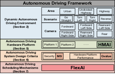
Figure 3: An overview of Framework in Autonomous Driving System.

We propose a synergistic framework for driving automation to bridge the gap between variable driving automation workloads and complicated hardware substrates, as shown in Figure 3. Specifically, we first propose a CNN taxonomy and design principles for hardware accelerators. Based on these knowledge, we propose a novel heterogeneous multi-core AI accelerator (HMAI) to provide the hardware substrate for the driving automation tasks with variability. Our framework also defines the system design criteria to better utilize hardware resources and achieve increased throughput while satisfying the performance and energy restrictions. Specifically, we propose two metrics, Matching Score (MS) and Global State Value (Gvalue) to formalize the criteria. MS pays attention to the safety requirements of various tasks in driving automation systems, while Gvalue puts more weight onto the overall performance of HMAI that reflects the globality. Finally, our framework employs a deep reinforcement learning (RL)-based task scheduling mechanism FlexAI to meet the system design criteria.

5 HMAI-A Heterogeneous Multicore AI Platform

In this section, we propose a heterogeneous multicore AI platforms (HMAI) tailored to the CNN-related perception tasks for driving automation framework. To achieve this goal, we first propose a taxonomy of existing accelerator architectures for CNNs and choose the best sub-accelerators for driving automation workloads based on the taxonomy. We then propose the architecture of HMAI that consists of three representative sub-accelerators.

5.1 A Taxonomy for CNN Accelerators

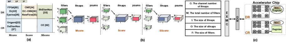
Figure 4: (a) Quadrant Classification for CNN accelerators[58, 59, 60, 61, 62, 63, 64, 65, 66, 67]. (b) Data processing style. (c) Register allocation.

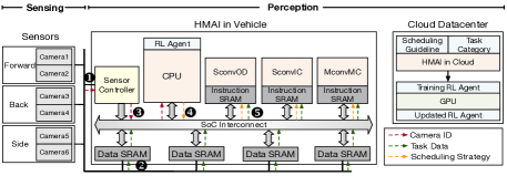
Figure 5: An overview of HMAI.

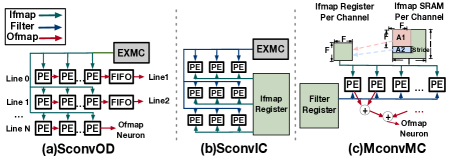
Figure 6: SconvOD, SconvIC and MconvMC in HMAI.

To choose the representative sub-accelerator architectures for HMAI, we need a comprehensive understanding of existing CNN accelerators as shown in Figure 4 (a). We propose a taxonomy for emerging CNN accelerators with respect to data processing style, register allocation, and data propagation types.

Data Processing Style. In this work, we first categorize the CNN accelerators into three styles as shown in Figure 4 (a), namely S(ingle)conv, S(pecial)Sconv and M(ultiple)conv according to their data processing methods. As shown in Figure 4 (b), Sconv processes a whole 2D convolution each iteration. While SSconv only processes a part of 2D convolution each iteration. For Mconv, it processes multiple 2D convolutions each iteration. We define the data processed by the accelerator in each iteration as a basic calculation unit (a.k.a., BasicUnit). For example, in Figure 4 (b), the size of filters in a BasicUnit of Mconv is $F\times F\times T_{m}\times T_{c}$, the size of ifmaps is $I\times I\times T_{c}$, and the size of psums is $O\times O\times T_{m}$.

Register Allocation. Figure 4 (c) illustrates a high-level block diagram of a typical CNN accelerator. It consists of an accelerator chip and an external memory chip (EXMC). Processing elements (PE) array is often used as the main functional component in the accelerator chip, which contains multiply-accumulate unit (MAC) as computation units. The on-chip buffer (OCB) is used to store ifmaps, filters, and psums. We classify the CNN accelerators into two categories with respect to register type: dispersive register (DR) and concentrated register (CR). In DR the registers are dispersed in each PE, while in CR a centralized storage is used and never stores psums. The size requirements of these registers are different among accelerators. Table 10 lists different structure designs for Sconv, SSconv and Mconv.

	EXMC	OCB	PE Register	MAC num in each PE
Sconv & SSconv	✓	$\times$	CR or DR	1
Mconv	✓	✓	CR or DR	>1

Table 10: Different structure design for Sconv, SSconv and Mconv.

Data Propagation Types. We further define three data propagation types for the data propagation between different PEs, Ofmaps Propagation (OP), Ifmaps Propagation (IP), and Multiple Propagation (MP). (1) For OP, the ifmaps are directly sent to PEs in one BasicUnit. The filters are fixed in the PEs in advance. The psums are accumulated during the data propagation between PEs. Upon all PEs are traversed, the ofmaps neuron is generated. (2) For IP, in one BasicUnit, the filters will be sent directly to the PEs. The ofmaps are fixed in PEs. The ifmaps propagate between PEs for reuse. (3) For MP, in one BasicUnit, there will be single or multiple types of data propagation between PEs. Figure 4 (a) shows typical CNN accelerators with different data propagation types. Note that data propagation always indicates data transfer between PEs’ registers. If there is no register in each PE, data propagation means data transfer between PE array and CR, since CR is equivalent to a collection of registers in each PE.

5.2 The Architecture of HMAI

Based on the above mentioned CNN accelerator taxonomy, we propose a heterogeneous multicore AI accelerator (HMAI) that contains three representative accelerators (SconvOD, SconvIC, MconvMC) in an automated vehicle. Each AI core has its specific architecture, as shown in Figure 6. Figure 6 shows the architecture and data/control flows in the HMAI: ❶cameras with different frame rate in the sensing component will generate multiple frames each time. After the cameras generate the frames data, they will signal the sensor controller with their ID separately and the sensor controller will launch DMA transition between camera and Data SRAM; ❷since each camera has its identical data SRAM, DMA will transfer the frame point to point, from a specific camera to its related data SRAM; ❸at the same time, CPU will acquire camera ID of current task from the controller through SoC interconnect; ❹ the well-trained RL agent in the CPU will generate a scheduling strategy for all tasks according to its camera ID, and then this strategy will be sent to a corresponding accelerator through interconnect (the RL agent can be retrained by GPU in cloud data center, when the task category and scheduling strategy need to be changed); ❺guided by the scheduling strategy, each accelerator will read the frame data from the corresponding SRAM and start the computation.

Why these accelerators? The HMAI is tailored to the CNN-related driving automation perception tasks. We choose to implement all data processing styles, the Sconv, SSconv and Mconv as described in Section 5.1. To cover all data propagation types in HMAI, we further choose to implement Sconv-OP, SSconv-IP and Mconv-MP based on multiple existing accelerator types as shown in Figure 4. To cover the register allocation methods, we implement SconvOD as Sconv-OP-DR, SconvIC as SSconv-IP-CR and MconvMC as Mconv-MP-CR.

The architecture design of sub-accelerators. As shown in Figure 6 (a), SconvOD is based on NewFlow [60]. In SconvOD, each ifmaps neuron only needs to be taken from the EXMC once. In each cycle, the same ifmaps neuron is sent to all PEs, but not every PE will generate a valid signal for this ifmaps. Different filter weights are fixed in different PE’s registers in advance. As to ofmaps neurons, it will be obtained after propagating to all PEs and FIFOs. The design of SonvIC is shown in Figure 6 (b), which is based on ShiDianNao [58]. In each cycle, the same filter weight is sent to all PEs. Different ifmaps neurons are read from the ifmaps register (the ifmaps register has the double buffer) to different PEs. Each PE computes only one output neuron each time. The design of MconvMC is based on Origami [66], and it is shown in Figure 6 (c), where its parameters of BasicUnit $T_{m}=T_{c}$. In ifmaps SRAM A1, the neurons of $T_{c}$ channels are sent to ifmaps register. Then the register sends ($F\times F\times T_{c}$)-size data to the PE array. Each PE will receive ($F\times F$)-size data, while the data in A2 will be sent to the register. For filters, different $F\times F$ are sent to different PEs at each cycle until all corresponding $T_{m}$-size filters are sent. In order to guarantee the pipelining, each PE will produce a result of matrix multiplication, and then the results in all PEs will be accumulated and sent out.

6 System Design Criteria

In this section, we propose Matching Score (MS) and Global State Value (Gvalue), to assist autonomous driving system guide the task execution on platforms.

6.1 Matching Score (MS)

Like Tesla (with 8 cameras), automated vehicles normally equip with multiple surrounding cameras to receive 360 degrees of visibility. As the different cameras have different max distance[23], each camera has its own requirement for their response time. This response time means automated vehicle’s processing time for each camera’s task. Based on the different camera’s response time, we define their matching score (MS). Specifically, we characterize the camera’s MS under object detection and object tracking tasks.

Matching Score - Object Detection Cameras in vehicles can be divided into three categories: forward, rear and side cameras. We first introduce the MS of forward cameras. When an obstacle is detected by a forward camera, this obstacle may be in one of the three states: (1) moving in the same direction as the vehicle, (2) standing still, and (3) moving in the opposite direction as the vehicle. Among those, the obstacle in the third state needs the shortest time to be detected, and we define this shortest time as the safety time of this forward camera.

Based on the Responsibility-Sensitive Safety (RSS) safety model[68], the safety time of each camera can be derived. RSS reveals the relationship between safe distances and processing time of vehicles in different scenarios. When the two vehicles are driving at opposite directions, [68] proposes the minimal safe distance $d_{min}$ between rear car $c_{1}$ and front car $c_{2}$ with velocities $v_{1}$ , $v_{2}$.

$$\scriptsize d_{min}=\left[\frac{v_{1}+v_{1,\rho}}{2}\rho+\frac{v_{1,\rho}^{2}}{2a_{min,brake,correct}}+\frac{\lvert v_{2}\rvert+v_{2,\rho}}{2}\rho+\frac{{v_{2,\rho}}^{2}}{2a_{min,brake}}\right]$$ (1)

In Equation(1), $\rho$ is the processing time of $c_{1}$, $a_{max,accel}$ is vehicle’s acceleration, $v_{1,\rho}=v_{1}+\rho a_{max,accel}$, and $v_{2,\rho}=\lvert v_{2}\rvert+\rho a_{max,accel}$. $a_{min,brake,correct}$ and $a_{min,brake}$ are the breaking acceleration of $c_{1}$ and $c_{2}$ respectively.

In this paper, we set $d_{min}$ to the max distance of each camera. $v_{1}$ and $v_{2}$ are the maximum velocity allowed in different areas (the maximum velocity in urban areas is 60km/h, undivided-highways is 80km/h and highways is 120km/h[69]). $a_{max,accel}$ of $c_{1}$ and $c_{2}$ is $8.382m/s^{2}$ which is the maximum acceleration of Tesla[23]. $a_{min,brake,correct}$ and $a_{min,brake}$ is $6.2m/s^{2}$, which is the maximum reasonably skilled driver’s braking acceleration[70]. Based on the above parameters, we can derive $\rho$, the safety time of forward cameras, so as to obtain the maximum response time allowed of each forward camera.

For the rear and side cameras, their safety time can be computed through Equation(1) like forward cameras. To be noted that: (1) reversing will not be considered on the highway; (2) the maximum velocity of turning is set to 50km/h[71]. In summary, different cameras have different safety time, thus the maximum response time allowed of different cameras are different. In this paper, we define the matching score (MS) to indicate the relationship between the response time and the safety time (maximum response time) of each camera.

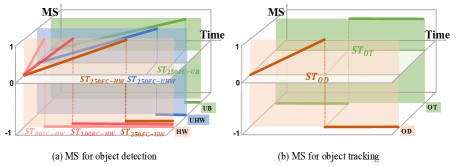
Figure 7: MS in automated vehicles.

In Figure 7(a), the horizontal axis represents the object detection tasks’ response time for each camera, and the vertical axis represents MS. First, we analyze the MS of the same camera in different driving scenarios. $ST_{250FC-HW}$, $ST_{250FC-UHW}$ and $ST_{250FC-UB}$ represent the safety time of a forward camera with maximum distance 250 meters in HW, UHW and UB. We define [$0-ST_{250FC-HW}$],[$0-ST_{250FC-UHW}$] and [$0-ST_{250FC-UB}$] as accepted time (ACTime) regions, while treating [$ST_{250FC-HW}-\infty$],[$ST_{250FC-UHW}-\infty$] and [$ST_{250FC-UB}-\infty$] as unaccepted time (UACTime) zones. If a response time for a task lies in the ACTime region, its MS grows linearly as the time increases. This is because the energy consumption of the hardware would reduce as the execution time increases while safety time is guaranteed in this region [72]. In the UACTime zone, the MS plummets to -1 due to the unacceptability of the response time. Furthermore, because the maximum velocity limit of the UB, UHW and HW is gradually increased, $ST_{250FC-UB}$, $ST_{250FC-UHW}$, and $ST_{250FC-HW}$ are gradually reduced accordingly.

Next, we introduce the MS for different cameras in the same driving scenario. As shown in Figure 7(a), $ST_{250FC-HW}$, $ST_{100RC-HW}$ and $ST_{80SC-HW}$ represent the safety time of forward camera, rear camera and side camera with a maximum distance of 250, 80 and 100 meters respectively in HW. [$0-ST_{250FC-HW}$],[$0-ST_{80SC-HW}$] and [$0-ST_{100RC-HW}$] are ACTime regions, while [$ST_{250FC-HW}-\infty$], [$ST_{80SC-HW}-\infty$] and [$ST_{100RC-HW}-\infty$] are UACTime zones. The trend of MS for these three cameras in ACTime and UACTime are the same as above.

Matching Score - Object Tracking This section will introduce cameras’ MS when its task type is object tracking. In the Figure 7(b), $ST_{OD}$ and $ST_{OT}$ is the safety time of the same camera when its task type is object detection (DET) and object tracking (TRA) respectively. In autonomous driving system, TRA follows DET to predict the trajectories of moving objects[14], which indicates that TRA is processed after DET for the same image. Therefore, $ST_{OT}$ should not be less than $ST_{OD}$, and we set $ST_{OT}$ equals to $ST_{OD}$ here. In the Figure 7(b), [$0-ST_{OT}$] is ACTime, and [$ST_{OT}-\infty$] is UACTime. When TRA’s response time of the current camera is in ACTime, MS is always -1, otherwise MS is 1.

6.2 Global State Value

To evaluate the overall performance of HMAI, we consider energy consumption $E$, runtime $T$ and resource utilization balance rate $R\_Balance$. $R\_Balance$ means the balance of resource utilization in HMAI, thus the higher $R\_Balance$, the less idle accelerators in HMAI at every moment. Whenever HMAI completes processing a task, these three values change accordingly. As the energy consumption of HMAI is expected to be as small as possible, the shorter the running time and the better the resource utilization balance rate to be, we define the Global State Value as $Gvalue=(-E-T+R\_Balance)/3$ (after normalization).

7 FlexAI-A Task Scheduling Engine

In the autonomous driving system, the dynamic environment can generate a massive amount of tasks, while the hardware resources are limited. Thus based on the metrics in criteria, how to designate tasks to different accelerators in HMAI needs to be carefully designed.

We use a real case to show the necessity of scheduling. Consider that when 30 cameras in a vehicle work once, then 30 frames will be generated simultaneously, thus we assume there will be 30 SSD tasks to process. We can not just allocate the same task to its best-fit accelerator because this will hurt the resource utilization of HMAI and overwhelm the chosen accelerator. Therefore, future driving automation platform needs an efficient task scheduling mechanism to trade-off among execution time, energy consumption, resource utilization and matching score.

The scheduling problem faced by HMAI is NP-complete. Conventional algorithms used to solve it can be classified into two groups, the heuristic-based and guided random-search-based algorithms[57]. As for heuristic-based algorithms, [47] proposed the Adaptive Task-partitioning Algorithm (ATA) to find out the scheduling policy of a task to consume as little energy as possible while guaranteeing the latency. The Min-min algorithm is considered as optimal in [46]. However, this algorithm can only consider the best hardware for each task while neglecting the global performance of HMAI.

Genetic algorithms (GAs)[54, 55, 56] and simulated annealing (SA)[73, 74] are the most popular and widely used techniques for task scheduling problems in guided random-search-based algorithms. However, a fitness equation in GA and a cost function in SA are needed to select the optimal strategy for current tasks, thus the global performance like resource utilization of HMAI can’t be taken into account.

In this paper, we propose FlexAI, a learning-based task scheduler to resolve the scheduling issues in driving automation system. Table 11 compares our work with other algorithms with respect to the coverage of the metrics proposed in Section 6. Specifically, to perceive the global performance in HMAI, we will use deep reinforcement learning (RL)[75] in FlexAI as the scheduling algorithm introduced in Section 7.1. In Section 7.2, we will introduce how to use scheduling metrics to get the reward in RL.

Metrics	Heuristic				Random-search		FlexAI
	EDP[53]	Min-Min[46]	ATA[47]	W-rand[76]	GA[57]	SA[74]
Time	✓	✓	$\times$	✓	✓	✓	✓
Energy	✓	✓	✓	✓	✓	✓	✓
Resrc	$\times$	$\times$	$\times$	$\times$	$\times$	$\times$	✓
MS	$\times$	✓	✓	$\times$	✓	✓	✓

Table 11: The metrics of some algorithms and FlexAI.

7.1 How the RL Agent Works

We propose a reinforcement learning (RL)-based algorithm for task scheduling on the HMAI. A RL agent can learn strategy by interacting with the environment without any supervision. In each episode of learning, the agent can provide decision-making policies according to the current environment (HMAI) and the long-term objective. This is done by receiving feedback in form of a reward from the environment.

Assuming there are $N$ CNN accelerators {$H_{1}$, $H_{2}$ … $H_{N}$} in the HMAI, and there will be $M$ tasks {$A_{1}$, $A_{2}$ … $A_{M}$} coming in sequence, of which each is a CNN-based task like object detection based on YOLO or SSD, object tracking based on GOTURN. Then, the proposed RL algorithm generates scheduling strategy P = {$p_{1}$, $p_{2}$ … $p_{M}$}, each of which indicates the task $A_{i}$ will be scheduled to $H_{j}$ under the guidance of $p_{i}$. When $A_{i}$ is executed, the metrics of HMAI will be updated accordingly, and the difference between the updated value and the previous value is denoted by reward $r_{i}$, thus the corresponding reward set is {$r_{1}$, $r_{2}$ … $r_{M}$}.

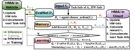
Figure 8: The work flow of the RL scheduling agent.

The RL agent input contains three parts when training: (1) Task-Info including three parameters: Amount: the computation amount when task is processed; LayerNum: the CNN layer’s number in the task; safety time: described in the Section 6.1. (2) HW-Info: the current information of all accelerators in the HMAI (the parameters of HW-Info will be described in Section 7.2). (3) Reward, in inference, there is no reward because the network doesn’t need to update.

In this paper, we will use DQN to learn scheduling strategy from episodic job queues. [77] divided the RL algorithm into three categories: critic-only (e.g. DQN [12]), actor-only (e.g. Policy gradient [78]) and actor-critic (e.g. DDPG [79]). When the scheduling strategy of a single task is generated, the critic-only algorithm can be trained once directly. However, the actor-only algorithm can only be trained after the scheduling strategies of all tasks in a task queue are generated. Since the number of tasks in each task queue in autonomous driving system is extremely large (up to 30,000 introduced in Section 8.3), to reduce training time, we will not choose actor-only category. Furthermore, although actor-critic can be trained in the same way as critic-only, due to its high computation complexity, we will choose DQN that falls into the critic-only category.

In our method, the two networks are denoted by EvalNet $D_{1}$ with the parameter $\theta_{1}$ and TargNet $D_{2}$ with the parameter $\theta_{2}$. EvalNet is used to generate the scheduling policy of the current task, while TargNet is used to update the parameters of the EvalNet. These two networks are consisting of two fully connected layers, and their input $S_{i}$ is Task-Info and HW-Info of task $A_{i}$. The output of these two networks is a group of Q values $Q_{j}$. $Q_{j}$ is the cumulative value of the reward: $Q_{j}=\sum_{{}^{n=i}}^{M}r_{n}$, which is generated after the task $A_{i}$ was executed on the $H_{j}$. After obtaining $N$ Q values, EvalNet or TargNet will choose $H_{j}$ which attains the maximum Q value after $A_{i}$ is executed. The choice $H_{j}$ of EvalNet or TargNet is a scheduling strategy $p_{i}$ which guides to schedule task $A_{i}$.

Figure 8 shows the working process of our RL scheduling agent. First, EvalNet $D_{1}$ will generate scheduling strategy for the input $S_{i}$, and use it to allocate task $A_{i}$ to $H_{j}$. Then, in training, (1) HMAI in cloud uses $H_{j}$ to update HW-Info, and calculates reward $r_{i}$. Next, HW-Info will combine with Task-Info of next task $A_{i+1}$ to generate $S_{i+1}$; (2) the record ($S_{i},H_{j},r{i},S_{i+1}$) is saved in memory, and if the total amount of records in the memory is greater than the memory size at this time, the RL agent will use $record_{m}$ - $record_{n}$ to start learning. (3) in learning, as for $record_{i}$, Eval_net $D_{1}$ will use $S_{i}$ to generate $Q_{i}$, and TargNet $D_{2}$ will use $S_{i+1}$ to generate $Q_{i+1}$. Then $\theta_{1}$ is updated by minimizing the loss: $L={(y_{i}-maxD_{1}(s_{i}|\theta_{1}))}^{2}$, where $y_{i}=r_{i}+\gamma maxD_{2}(s_{i+1}|\theta_{2})$. The parameter $\theta_{2}$ in $D_{2}$ will be copied directly from $D_{1}$ every fixed time. In inference, HMAI in vehicle uses $H_{j}$ to update HW-Info, and then $S_{i+1}$ is sent to the EvalNet $D_{1}$ directly.

7.2 The Way to Get Reward

In this section, we will introduce how to use scheduling metrics to get the reward in RL. Suppose that the information (Info) of $H_{i}$ is ($E_{i},T_{i},R\_Balance_{i},MS_{i}$), and we use Info for each accelerator in HMAI to constitute the HW-Info. After $A_{j}$ is scheduled to $H_{i}$, the energy consumption, time, MS and resources utilization balance rate of processing $A_{j}$ are denoted by $e_{j}$, $t_{j}$, $ms_{j}$ and $r_{j}$. Thus, for $H_{i}$, (1)$E_{i}+=e_{j}$; (2)$T_{i}+=t_{j}$; (3)$MS_{i}+=ms_{j}$; (4)$R\_Balance_{i}=\frac{r_{j}+R\_Balance_{i}}{num}$ (num is the number of tasks has been executed in $H_{i}$). Until now, the energy consumed in each accelerator is $\{E_{1},E_{2}...E_{N}\}$ respectively, the total time is $\{T_{1},T_{2}...T_{N}\}$, the resource utilization is $\{R\_Balance_{1},R\_Balance_{2}...R\_Balance_{N}\}$, and the sum of the $MS$ in each accelerator is $\{MS_{1},MS_{2}...MS_{N}\}$. Then for HMAI, (1) $E=\sum_{i=1}^{N}E_{i}$; (2) $R\_Balance=\frac{1}{N}\sum_{i=1}^{N}{R\_Balance_{i}}$; (3) $MS=\sum_{i=1}^{N}MS_{i}$; (4) $T=\max\{T_{1},T_{2}...T_{N}$}.

Now if there are currently $M-1$ tasks scheduled to HMAI, at this moment, the HMAI has $E$, $T$, $R\_Balance$, and $MS$. When the $Mth$ task is executed, the four values will be updated to $E_{new}$, $T_{new}$, $R\_Balance_{new}$, and $MS_{new}$. Then, after processing $Mth$ tasks reward is given by $(-E_{new}-T_{new}+R\_Balance_{new})/3-(-E-T+R\_Balance)/3+MS_{new}-MS=Gvalue_{new}-Gvalue+MS_{new}-MS$.

8 Evaluation

Parameter	Description
Camera_HZ(A, S, C)	A includes UB, UHW, HW
	S includes Go straight, Turn and Reverse
	C includes FC, FLSC,RLSC, FRSC, RRSC and RC
MaxTimes_Turn(A)	A includes UB, UHW, HW
MaxTimes_Reverse(A)	A includes UB, UHW, HW
MaxDuration_Turn(A)	A includes UB, UHW, HW
MaxDuration_Reverse(A)	A includes UB, UHW, HW
Velocity(A)	A includes UB, UHW, HW
Safety_Time(A, C)	A includes UB, UHW, HW
	C includes FC, FLSC,RLSC, FRSC, RRSC and RC

Table 12: The parameters in Autonomous Driving Environment.

8.1 The Dynamic Driving Environments

To simulate a variety of vehicle driving areas and scenarios, we define several parameters (listed in Table 12), which characterize dynamic driving environments. Note that when the parameter A (urban areas (UB), undivided-highways (UHW), highways (HW)) changes, the frequency of cameras (Camera_HZ), the maximum number of turning ((MaxTimes_Turn) and reversing (MaxTimes_Reverse), the longest duration of turning (MaxDuration_Turn) and reversing (MaxDuration_Reverse), the speed of the vehicle (Velocity), and the safety time of cameras (Safety_Time) will all change. Moreover, when the parameter C (FC, FLSC, RLSC, FRSC, RRSC and RC) changes, Camera_HZ and Safety_Time will vary. Similarly, when the parameter S (Go straight, Turn and Reverse) changes, Camera_HZ will change also. Table 4 lists the number of cameras in each type.

Parameter Setting
MaxTime_Turn	10
MaxTimes_Reverse	10
MaxDuration_Turn	10
MaxDuration_Reverse	20
Current Setting
Turn Times	2
Reverse Times	1
Turn Duration	3s,4s
Reverse Duration	2s

Table 13: The parameters.

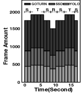
Figure 9: The task queue.

Task Queue. In this experiment, we use images in the KITTI object tracking 2D dataset [80] as tasks in our task queue. This object tracking dataset consists of multiple sequences, and the images in each sequence are the continuous outputs for one camera in our vehicle. Based on the parameters in Table 12, we create different driving routes with various driving distances, and all tasks generated by the vehicle during the route form one task queue. In addition to the dataset that constitutes the task queue, we also specify the task amount at different time in this task queue. Figure 8.1 illustrate an example of a task queue when a vehicle has a 160m route in UB and its velocity is 20m/s. Parameters such as Camera_HZ, Safety_Time are derived from Figure 1, Section 6.1 and Table 8.1. As mentioned in Section 2, we alternately use YOLO and SSD to process the DET tasks for each camera, and use GOTURN to process TRA tasks, thus the task types in Figure 8.1 are YOLO, SSD and GOTURN. In Figure 8.1, S, T and R indicate three scenarios: going straight, turning and reversing, and the start time and lasting time of each scenario is randomly determined.

8.2 Performance Analysis for HMAI

The construction of HMAI. In Figure 2 (b), we give the resource utilization rate of each platform in urban areas. Comparing the geometric mean of resource utilization rates in three scenarios of each platform, we find (4 SconvOD, 4 SconvIC, 3 MconvMC) is the best configuration. According to the same method, in the other two areas, above heterogeneous platform configuration can also achieve optimal resource utilization. Therefore, we choose to use (4 SconvOD, 4 SconvIC, 3 MconvMC) to construct our heterogeneous platform HMAI.

Experimental Methodology. The performance and energy of HMAI is measured by the following tools. For the performance evaluation, a customized cycle-accurate simulator was designed and implemented to measure execution time in number of cycles. This simulator models the microarchitectural behavior of each hardware module of our design. In addition, we use ARM1176 as the main control processor in the HMAI to do task scheduling.

For measuring area and power, we implemented a Verilog version of each hardware module, then synthesized it. We used the Synopsys Design Compiler with the TSMC 12nm standard VT library for the synthesis, and estimated the power consumption using Synopsys PrimeTime PX. In addition, the design of SconvOD, SconvIC and MconvMC is based on  [60, 58, 66]. And the SRAM is generated by Synopsys Memory Compiler and the interconnect bus is generated by Synopsys DesignWare AMBA IP.

Baseline. To compare HMAI with state-of-the-art work, we evaluate HMAI with NVIDIA Tesla T4 GPU, which is mainly designed for AI inference workloads. In addition, in order to prove that heterogeneous platform is better than homogeneous platform, we compare the performance of HMAI with multiple homogeneous platforms. The homogeneous platforms compared here have been mentioned in Section 3.1, which are 13 SconvOD, 13 SconvIC and 12 MconvMC.

The Parameters for Constructing Task Queue and Experimental Methodology. Here, we create different driving routes for urban area (UB) with various distances from 1km to 2km, and vehicle’s velocity is set to 60km/h. In Experimental, first, 5 task queues are constructed, and then we use HMAI including FlexAI, NVIDIA Tesla T4 and three homogeneous platforms to process each task queue.

Experimental Results. We first compare the performance speedup normalized to Tesla T4, as shown in Figure 10 (a). Overall, HMAI achieves 5× speedup over Tesla T4, since HMAI provides more sufficient computing units for autonomous driving performance requirements. Note that, different autonomous driving scenarios have different performance requirements (detail in Section 3.1). In order to satisfy all requirements, the computing resources in the homogeneous platforms will be redundancy in some scenarios, thus there will be a task which response time is much shorter than its safety time. Therefore in Figure 10 (a), all homogeneous platforms achieve higher speedup compared to HMAI. However, in various driving scenarios, by reasonably using the computing resources in heterogeneous HMAI, HMAI will have high resource utilization rate as shown in Figure 2 (b) and safe response time for each task.

Figure 10 (b) shows the normalized power of HMAI and the the homogeneous platforms, normalized to Tesla T4. HMAI reduces power by 57%, 30% and 33% compared to three homogeneous platforms on average. The main reason is the reduction of a large number of redundancy computing resources. Since HMAI has much more computing resources than Tesla T4, it has about 2× power over Tesla T4. Theoretically, 5 Tesla T4 can have sufficient performance for autonomous driving, while the corresponding power will also be increased 5× than Tesla T4 itself. Here HMAI has only 2× power over Tesla T4, thus in Figure 10 (c), HMAI has higher TOPS/W than Tesla T4. In Figure 10 (c), HMAI also has higher TOPS/W than three homogeneous platforms due to its high resource utilization rate.

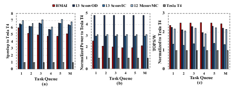
Figure 10: Comparison between HMAI and baselines. The last set of bars, labeled as M, indicate the geometric mean across all task queues.

8.3 Performance Analysis for FlexAI

In this section, we set up experiments to compare our RL-based FlexAI with other state-of-the-art schedulers.

Baseline. We use Min-Min, ATA in heuristics, GA, SA in guided random search techniques, as well as the unscheduled worse case as our baselines.

The Parameters for Constructing Task Queue. We create different driving routes for urban area (UB), undivided-highways (UHW), and highways (HW) with various distances from 1km to 2km, and velocity is set to 60km/h, 80km/h and 120km/h respectively[69].

Training. The DQN used in FlexAI agent includes two networks with exactly the same structure but different updating paces. Each network is comprised of two fully connected layers, and a softmax layer. The number of neurons of the fully connected layers are 256 and 64 with ReLU non-linearity. We train three RL agents for UB, UHW, and HW respectively. Each agent is trained on the NVIDIA TITAN-XP with 1000 episodes, and each episode includes one task queue. The learning rate for training the EvalNet is 0.01.

Training Loss Curve. Figure 11 shows the training loss curve of FlexAI RL agent in urban area. Each iteration represents one task, and each episode contains one task queue. As all object detection and object tracking tasks generated by a vehicle in a 1km - 2km route will form one task queue, each episode will contain up to 30,000 tasks. In Figure 11, the loss of the second episode gradually stabilizes after 10,000 iterations, while in the third and fourth episodes, except for the loss of the initial 2,000 iterations, the subsequent loss gradually tends to 0. The reason for that is the composition of tasks in each episode are very similar, thus the network trained in prior episodes will be applicable to subsequent episodes. This also further illustrates that if the task types do not change, the well-trained RL agent can be used all the time in automated vehicles.

Experimental Methodology. For each area, first we use well-trained agent of FlexAI and each baseline to generate the scheduling strategy for 5 task queues. Next we compare the metrics between FlexAI and baselines for each task queue.

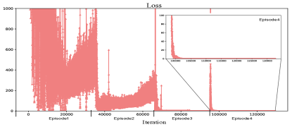
Figure 11: Loss curve of RL agent. The threshold of the y-axis is 1000.

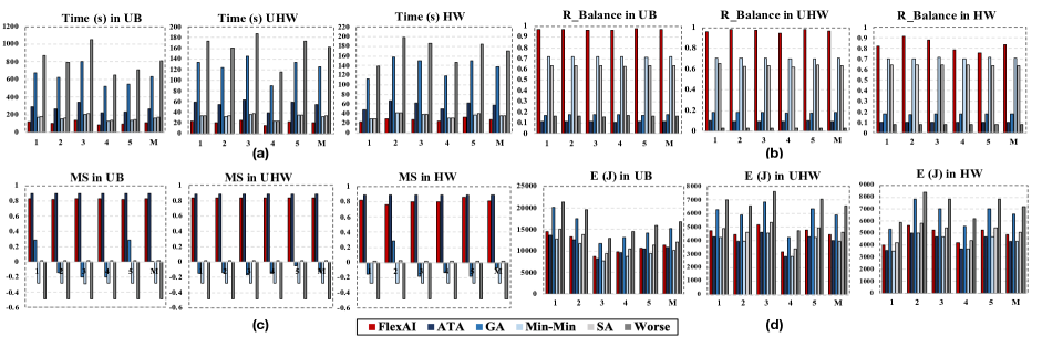
Figure 12: Comparison between FlexAI and baselines. UB, UHW and HW means urban areas, undivided-highways and highways. M is the geometric mean of 5 task queues.

Experimental Results.The time in Figure 12 includes three parts: (1) scheduling strategy runtime in CPU, (2) task waiting time and (3) task execution time. In Figure 12(a), FlexAI can maximally reduce the time by 60%, 88%, 33%, 36% and 87% compared to ATA, GA, Min-Min, SA and worse case in urban area. And for the geometric mean, FlexAI decreases at most 87%. The reason for this is FlexAI can effectively reduce the task waiting time, and more details can be found in Section 8.4. For Min-Min, SA and ATA, they perform close to the FlexAI does since they consider execution time when scheduling. However, due to the fact that GA’s performance is affected by the selection of the initial population, its time is much large than FlexAI. To summary, FlexAI can always achieve the minimum time in three areas, and this will ensure the safety of autonomous driving.

As shown in Figure 12(b), the $R\_Balance$ of FlexAI has been maximally improved by 837%, 957%, 62%, 55% and 960% compared to ATA, GA, Min-Min, SA and worse case in urban area. As for the geometric mean in all areas, $R\_Balance$ in FlexAI is always the best. This is because among all scheduling strategies, only FlexAI considers the balance of resource utilization. The situation of $R\_Balance$ in the other two areas is the same as the urban area. In HMAI, by increasing $R\_Balance$, the task waiting time can be reduced, and at the same time it can decrease the waste of the hardware resources and improve the vehicle’s endurance.

In Figure 12(c), MS in FlexAI is larger than that in GA, Min-min, SA and worse case (up to 1.02, 1.12, 0.83, 1.32), however smaller than that in ATA in the urban area. The reason is ATA is optimized towards MS, but FlexAI needs to tradeoff among four metrics. In addition, except for ATA and FlexAI, the other baselines’ MS are always less than 0, which means there are many tasks in each task queue whose processing time are greater than the safety time. The situation of MS in the other two areas is the same as the urban area. In autonomous driving, higher MS represents better safety, and more discussion can be found in Section 8.4.

Figure 12(d) shows the comparison of energy. Although FlexAI can achieve lower energy than GA, SA and worst case in all areas, it is slightly higher than the others. Some reasons are as follow. First, energy-performance tradeoff is common in accelerators. Moreover, FlexAI needs to consider $T$, $E$, $R\_Balance$ and MS at the same time, which makes tradeoff more difficult.

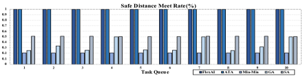
Figure 13: Safe distance meet rate (STMRate).

8.4 Autonomous Driving Metrics

Safety Time Meet Rate As we mentioned in Section 6.1, since each camera in a vehicle has a corresponding safety time, each task will have its safety time according to the camera that generated it. In this section, we define safety time meet rate (STMRate) to describe the proportion of tasks in a task queue whose processing time is less than its safety time. In Figure 13, for each task queue, the STMRate of FlexAI is basically close to 100%, which means the processing time of almost all tasks can ensure the driving safety. The reason for that is FlexAI considers MS when generating scheduling strategies, and MS indicates the relationship between the task processing time and task safety time. Here, since ATA is optimized towards MS, the STMRate of each task queue is also very high under ATA.

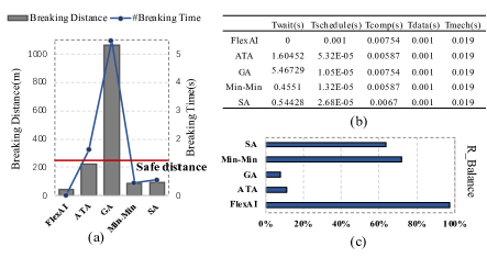
Figure 14: (a)Breaking distance and total breaking time; (b)Total breaking time breakdown; (c)R_Balance.

Braking Distance. Here, we assume that after a vehicle moves 1km, its forward camera finds there is an object 250 meters away, so it needs to take braking immediately. The current velocity of the vehicle is 60 km/h, and the braking deceleration is 6.2 $m/s^{2}$. In Figure 14 (a)(bar), the breaking distances under different schedulers are presented.

As shown in Figure 14 (a)(bar), except for GA, the breaking distances of other schedulers are all less than the safe distance 250 m, and FlexAI has the smallest breaking distance 47.08 m. Since the breaking distance is strongly related to the braking time (breaking distance is calculated based on the Equation(1) in Section 6), FlexAI has the smallest breaking time, as shown in Figure 14 (a)(blue line).

The total breaking time breakdown of each scheduler is shown in Figure 14 (b). $T_{wait}$ is the waiting time of the current task (the current task is used to detect the object that caused the braking); $T_{schedule}$ represents the runtime of each scheduler; $T_{compute}$ is the processing time of the current task in HMAI; $T_{data}$ is the time which is used to transmit the control commands to the vehicle’s actuator through the Controller Area Network (CAN) bus, which is 1 ms in this vehicle[81]; $T_{mech}$ is the time that mechanical components of the vehicle takes to start reacting, which is 19 ms. In Figure 14 (b), $T_{wait}$ in FlexAI is 0, while $T_{wait}$ is much larger than the time of other parts in other schedulers. Therefore, although $T_{schedule}$ and $T_{compute}$ of FlexAI are not the best, the total breaking time of FlexAI is the smallest.

Note that in our experiment, the vehicle generates a task queue from starting to braking. As shown in Figure 14 (c), $R_{Balance}$ in FlexAI is the largest. It means under FlexAI, the resource utilization in HMAI is the most balanced, thus the number of idle accelerators in HMAI at every moment is the least as well. For instance, if task A has the fastest execution time in the accelerator A and accelerator A is currently busying, FlexAI will schedule task A to other idle accelerators to reduce its waiting time, while for Min-Min, task A will be waiting until accelerator A changes to idle. Therefore, for FlexAI, since it has the highest $R\_Balance$, its $T_{wait}$ in Figure 14 (b) is the smallest. And under the smallest $T_{wait}$, FlexAI has the smallest braking distance in Figure 14 (a)(bar).

9 Related Work

To the best of our knowledge, an emerging line of research has found that reinforcement learning proves to be effective in solving scheduling problems in various domains. [82] uses RL to make real-time decision for the scheduling problem in flying mobile edge computing platform, and the reward of this RL agent includes the energy consumption of all user equipment. [83] proposes a multi-agent reinforcement learning approach for job scheduling in grid computing, of which the reward consists of the total execution time of all jobs. [84] uses RL to deal with the radar resource management problem when the radar assigns limited time resource to a set of tasks, and the reward is comprised of the number of tasks delayed or dropped. For mobile-edge computing system, [85] proposes a RL based task scheduling algorithm, with its reward involving the slowdown and average timeout period of tasks.

As the rewards of the algorithms aforementioned are designed for their specific scenarios, these ad-hoc formulations cannot be used to solve the scheduling problem in autonomous driving. In autonomous driving systems, each CNN-based task should be handled separately, and the reward should take into account not only the dynamic changes of the environment (HMAI), such as current resource utilization, but also the total energy consumption and the longest execution time among all accelerators. Furthermore, whether the current strategy meets the real-time requirements of the cameras in autonomous vehicles also matters. Therefore, it is desirable to develop RL-based scheduling algorithms for autonomous driving.

10 Conclusion

By exploring the variability of workloads and performance requirements in driving automation and the heterogeneity of multi-accelerators, we purpose a comprehensive framework that synergistically handles the heterogeneous hardware accelerator design principles, system design criteria, and task scheduling mechanism. First, based on a taxonomy for emerging CNN accelerators, we design a heterogeneous multicore AI platform (HMAI) which adopts three typical CNN accelerator architectures. Next, by designing two metrics: Matching Score and Global State Value, autonomous driving system can guide the task execution on the platform. Finally, FlexAI-a reinforcement learning-based mechanism are proposed to generate scheduling policies in autonomous driving.

References

- [1] “EyeQ3 - Mobileye - WikiChip.” [Online]. Available: https://en.wikichip.org/wiki/mobileye/eyeq/eyeq3
- [2] T. Inc., “(TSLA) CEO Elon Musk on Q3 2018 Results - Earnings Call Transcript | Seeking Alpha.” [Online]. Available: https://seekingalpha.com/article/4214138-tesla-inc-tsla-ceo-elon-musk-q3-2018-results-earnings-call-transcript?part=single
- [3] “First picture of Tesla’s new Hardware 3 self-driving computer in the wild - Electrek.” [Online]. Available: https://electrek.co/2019/07/31/tesla-hardware-3-self-driving-computer-first-picture/
- [4] H. Robotics, “Journey™Automotive AI Processor Series,” 2019. [Online]. Available: https://en.horizon.ai/product/journey
- [5] G. Sistu, I. Leang, S. Chennupati, S. Milz, S. K. Yogamani, and S. A. Rawashdeh, “Neurall: Towards a unified model for visual perception in automated driving,” CoRR, vol. abs/1902.03589, 2019. [Online]. Available: http://arxiv.org/abs/1902.03589
- [6] M. Yang, S. Wang, J. Bakita, T. Vu, F. D. Smith, J. H. Anderson, and J.-M. Frahm, “Re-thinking cnn frameworks for time-sensitive autonomous-driving applications: Addressing an industrial challenge,” in 2019 IEEE Real-Time and Embedded Technology and Applications Symposium (RTAS). IEEE, 2019, pp. 305–317.
- [7] M. Slovick, “Autonomous Cars and Overcoming the Inadequacies of Road Mapping | u-blox.” [Online]. Available: https://www.u-blox.com/en/beyond/blog/guest-blogs/autonomous-cars-and-overcoming-inadequacies-road-mapping
- [8] C. Ding, S. Wang, N. Liu, K. Xu, Y. Wang, and Y. Liang, “Req-yolo: A resource-aware, efficient quantization framework for object detection on fpgas,” in Proceedings of the 2019 ACM/SIGDA International Symposium on Field-Programmable Gate Arrays, 2019, pp. 33–42.
- [9] D. T. Nguyen, T. N. Nguyen, H. Kim, and H.-J. Lee, “A high-throughput and power-efficient fpga implementation of yolo cnn for object detection,” IEEE Transactions on Very Large Scale Integration (VLSI) Systems, vol. 27, no. 8, pp. 1861–1873, 2019.
- [10] Y. Wang, “Putting the brain in driverless vehicles with MDC,” 2019. [Online]. Available: https://www.huawei.com/uk/about-huawei/publications/communicate/86/driverless-vehicles-with-mdc
- [11] M. D. Hill and V. J. Reddi, “Accelerator-level parallelism,” CoRR, vol. abs/1907.02064, 2019. [Online]. Available: http://arxiv.org/abs/1907.02064
- [12] H. van Hasselt, A. Guez, and D. Silver, “Deep reinforcement learning with double q-learning,” in Proceedings of the Thirtieth AAAI Conference on Artificial Intelligence, February 12-17, 2016, Phoenix, Arizona, USA., 2016, pp. 2094–2100.
- [13] “Facts + statistics: Highway safety.” [Online]. Available: https://www.iii.org/fact-statistic/facts-statistics-highway-safety
- [14] S. Lin, Y. Zhang, C. Hsu, M. Skach, M. E. Haque, L. Tang, and J. Mars, “The architectural implications of autonomous driving: Constraints and acceleration,” in Proceedings of the Twenty-Third International Conference on Architectural Support for Programming Languages and Operating Systems, ASPLOS 2018, Williamsburg, VA, USA, March 24-28, 2018, 2018, pp. 751–766.
- [15] “Multi-task learning in the wilderness.” [Online]. Available: https://slideslive.com/38917690/multitask-learning-in-the-wilderness
- [16] Y. Zhou and O. Tuzel, “Voxelnet: End-to-end learning for point cloud based 3d object detection,” in Proceedings of the IEEE Conference on Computer Vision and Pattern Recognition, 2018, pp. 4490–4499.
- [17] J. Redmon and A. Farhadi, “Yolo9000: better, faster, stronger,” in Proceedings of the IEEE conference on computer vision and pattern recognition, 2017, pp. 7263–7271.
- [18] C.-Y. Fu, W. Liu, A. Ranga, A. Tyagi, and A. C. Berg, “Dssd: Deconvolutional single shot detector,” arXiv preprint arXiv:1701.06659, 2017.
- [19] D. Held, S. Thrun, and S. Savarese, “Learning to track at 100 FPS with deep regression networks,” in Computer Vision - ECCV 2016 - 14th European Conference, Amsterdam, The Netherlands, October 11-14, 2016, Proceedings, Part I, 2016, pp. 749–765.
- [20] W. Liu, D. Anguelov, D. Erhan, C. Szegedy, S. Reed, C.-Y. Fu, and A. C. Berg, “Ssd: Single shot multibox detector,” in European conference on computer vision. Springer, 2016, pp. 21–37.
- [21] A. Geiger, P. Lenz, C. Stiller, and R. Urtasun, “Vision meets robotics: The kitti dataset,” The International Journal of Robotics Research, vol. 32, no. 11, pp. 1231–1237, 2013.
- [22] T.-Y. Lin, M. Maire, S. Belongie, J. Hays, P. Perona, D. Ramanan, P. Dollár, and C. L. Zitnick, “Microsoft coco: Common objects in context,” in European conference on computer vision. Springer, 2014, pp. 740–755.
- [23] “Autopilot in tesla.” https://www.tesla.com/autopilot, 2019.
- [24] “Audi at ces las vegas 2020,” https://www.audi-mediacenter.com/en/audi-at-ces-las-vegas-2020-12457, 2020.
- [25] “Computer vision for autonomous driving: Keep an eye on the road,” https://www.intellias.com/computer-vision-keep-sharp-eye-road/, 2018.
- [26] “Uber’s use of fewer safety sensors prompts questions after arizona crash,” https://www.reuters.com/article/us-uber-selfdriving-sensors-insight/ubers-use-of-fewer-safety-sensors-prompts-questions-after-arizona-crash-idUSKBN1H337Q/, 2018.
- [27] “Waymo’s next-generation self-driving system can ‘see’ a stop sign 500 meters away,” https://www.theverge.com/2020/3/4/21165014/waymo-fifth-generation-self-driving-radar-camera-lidar-jaguar-ipace/, 2020.
- [28] “Self-driving carts to make their debut on uc san diego roads in january.” http://jacobsschool.ucsd.edu/news/news_releases/release.sfe?id=2350, 2017.
- [29] “Illinois to develop testing program for self-driving vehicles,” https://www.chicagotribune.com/news/ct-biz-illinois-self-driving-vehicles-20181025-story.html, 2018.
- [30] “Texas am launches autonomous shuttle project in downtown bryan,” https://engineering.tamu.edu/news/2018/10/texas-am-launches-autonomous-shuttle-project-in-downtown-bryan.html, 2018.
- [31] H. Zhao, Y. Zhang, P. Meng, H. Shi, L. E. Li, T. Lou, and J. Zhao, “Towards safety-aware computing system design in autonomous vehicles,” arXiv preprint arXiv:1905.08453, 2019.
- [32] A. Driving, “Levels of driving automation are defined in new sae international standard j3016: 2014,” SAE International: Warrendale, PA, USA, 2014.
- [33] E. Yurtsever, J. Lambert, A. Carballo, and K. Takeda, “A survey of autonomous driving: common practices and emerging technologies,” arXiv preprint arXiv:1906.05113, 2019.
- [34] “The driver assistance systems from audi: New concepts for safety, convenience and light,” https://www.audiusa.com/newsroom/news/press-releases/2011/11/driver-assistance-systems-from-audi-new-concepts-safety, 2011.
- [35] “Where’s what tesla’s dashcam using autopilot cameras looks like,” https://www.teslarati.com/tesla-dashcam-autopilot-cameras-first-look/, 2018.
- [36] A. Geiger, P. Lenz, and R. Urtasun, “Are we ready for autonomous driving? the kitti vision benchmark suite,” in 2012 IEEE Conference on Computer Vision and Pattern Recognition. IEEE, 2012, pp. 3354–3361.
- [37] X. Huang, P. Wang, X. Cheng, D. Zhou, Q. Geng, and R. Yang, “The apolloscape open dataset for autonomous driving and its application,” arXiv preprint arXiv:1803.06184, 2018.
- [38] C. Chen, A. Seff, A. Kornhauser, and J. Xiao, “Deepdriving: Learning affordance for direct perception in autonomous driving,” in Proceedings of the IEEE International Conference on Computer Vision, 2015, pp. 2722–2730.
- [39] A. Broggi, M. Buzzoni, S. Debattisti, P. Grisleri, M. C. Laghi, P. Medici, and P. Versari, “Extensive tests of autonomous driving technologies,” IEEE Transactions on Intelligent Transportation Systems, vol. 14, no. 3, pp. 1403–1415, 2013.
- [40] W. Maddern, G. Pascoe, C. Linegar, and P. Newman, “1 year, 1000 km: The oxford robotcar dataset,” The International Journal of Robotics Research, vol. 36, no. 1, pp. 3–15, 2017.
- [41] E. Santana and G. Hotz, “Learning a driving simulator,” arXiv preprint arXiv:1608.01230, 2016.
- [42] J. Redmon, S. Divvala, R. Girshick, and A. Farhadi, “You only look once: Unified, real-time object detection,” in Proceedings of the IEEE conference on computer vision and pattern recognition, 2016, pp. 779–788.
- [43] T. B. Preußer, G. Gambardella, N. Fraser, and M. Blott, “Inference of quantized neural networks on heterogeneous all-programmable devices,” in 2018 Design, Automation & Test in Europe Conference & Exhibition (DATE). IEEE, 2018, pp. 833–838.
- [44] H. Nakahara, H. Yonekawa, T. Fujii, and S. Sato, “A lightweight yolov2: A binarized cnn with a parallel support vector regression for an fpga,” in Proceedings of the 2018 ACM/SIGDA International Symposium on field-programmable gate arrays, 2018, pp. 31–40.
- [45] Y. Wang, S. Liang, S. Yao, Y. Shan, S. Han, J. Peng, and H. Luo, “Reconfigurable processor for deep learning in autonomous vehicles,” 2017.
- [46] T. D. Braun, H. J. Siegel, N. Beck, L. Bölöni, M. Maheswaran, A. I. Reuther, J. P. Robertson, M. D. Theys, B. Yao, D. A. Hensgen, and R. F. Freund, “A comparison of eleven static heuristics for mapping a class of independent tasks onto heterogeneous distributed computing systems,” J. Parallel Distrib. Comput., vol. 61, no. 6, pp. 810–837, 2001.
- [47] E. Oh, W. Han, E. Yang, J. Jeong, L. Lemi, and C. Youn, “Energy-efficient task partitioning for cnn-based object detection in heterogeneous computing environment,” in International Conference on Information and Communication Technology Convergence, ICTC 2018, Jeju Island, Korea (South), October 17-19, 2018, 2018, pp. 31–36.
- [48] S. K. Baruah, “Task partitioning upon heterogeneous multiprocessor platforms,” in 10th IEEE Real-Time and Embedded Technology and Applications Symposium (RTAS 2004), 25-28 May 2004, Toronto, Canada, 2004, pp. 536–543.
- [49] M. K. Rafsanjani and A. K. Bardsiri, “A new heuristic approach for scheduling independent tasks on heterogeneous computing systems,” International Journal of Machine Learning and Computing, vol. 2, no. 4, p. 371, 2012.
- [50] Z. Chen and D. Marculescu, “Priority-aware near-optimal scheduling for heterogeneous multi-core systems with specialized accelerators,” CoRR, vol. abs/1712.03246, 2017.
- [51] A. A. Khokhar, V. K. Prasanna, M. E. Shaaban, and C. Wang, “Heterogeneous computing: Challenges and opportunities,” IEEE Computer, vol. 26, no. 6, pp. 18–27, 1993.
- [52] O. H. Ibarra and C. E. Kim, “Heuristic algorithms for scheduling independent tasks on nonidentical processors,” J. ACM, vol. 24, no. 2, pp. 280–289, 1977.
- [53] T. Hamano, T. Endo, and S. Matsuoka, “Power-aware dynamic task scheduling for heterogeneous accelerated clusters,” in 23rd IEEE International Symposium on Parallel and Distributed Processing, IPDPS 2009, Rome, Italy, May 23-29, 2009, 2009, pp. 1–8.
- [54] E. S. Hou, N. Ansari, and H. Ren, “A genetic algorithm for multiprocessor scheduling,” IEEE Transactions on Parallel and Distributed systems, vol. 5, no. 2, pp. 113–120, 1994.
- [55] P. Shroff, D. W. Watson, N. S. Flann, and R. F. Freund, “Genetic simulated annealing for scheduling data-dependent tasks in heterogeneous environments,” in 5th Heterogeneous Computing Workshop (HCW’96), 1996, pp. 98–117.
- [56] R. C. Correa, A. Ferreira, and P. Rebreyend, “Integrating list heuristics into genetic algorithms for multiprocessor scheduling,” in Proceedings of SPDP’96: 8th IEEE Symposium on Parallel and Distributed Processing. IEEE, 1996, pp. 462–469.
- [57] H. Topcuoglu, S. Hariri, and M.-y. Wu, “Performance-effective and low-complexity task scheduling for heterogeneous computing,” IEEE transactions on parallel and distributed systems, vol. 13, no. 3, pp. 260–274, 2002.
- [58] Z. Du, R. Fasthuber, T. Chen, P. Ienne, L. Li, T. Luo, X. Feng, Y. Chen, and O. Temam, “Shidiannao: shifting vision processing closer to the sensor,” in Proceedings of the 42nd Annual International Symposium on Computer Architecture, Portland, OR, USA, June 13-17, 2015, 2015, pp. 92–104.
- [59] C. Farabet, C. Poulet, J. Y. Han, and Y. LeCun, “CNP: an fpga-based processor for convolutional networks,” in 19th International Conference on Field Programmable Logic and Applications, FPL 2009, August 31 - September 2, 2009, Prague, Czech Republic, 2009, pp. 32–37.
- [60] C. Farabet, B. Martini, B. Corda, P. Akselrod, E. Culurciello, and Y. LeCun, “Neuflow: A runtime reconfigurable dataflow processor for vision,” in IEEE Conference on Computer Vision and Pattern Recognition, CVPR Workshops 2011, Colorado Springs, CO, USA, 20-25 June, 2011, 2011, pp. 109–116.
- [61] S. T. Chakradhar, M. Sankaradass, V. Jakkula, and S. Cadambi, “A dynamically configurable coprocessor for convolutional neural networks,” in 37th International Symposium on Computer Architecture (ISCA 2010), June 19-23, 2010, Saint-Malo, France, 2010, pp. 247–257.
- [62] W. Qadeer, R. Hameed, O. Shacham, P. Venkatesan, C. Kozyrakis, and M. Horowitz, “Convolution engine: balancing efficiency and flexibility in specialized computing,” Commun. ACM, vol. 58, no. 4, pp. 85–93, 2015.
- [63] Y. Chen, T. Krishna, J. S. Emer, and V. Sze, “Eyeriss: An energy-efficient reconfigurable accelerator for deep convolutional neural networks,” J. Solid-State Circuits, vol. 52, no. 1, pp. 127–138, 2017.
- [64] C. Zhang, P. Li, G. Sun, Y. Guan, B. Xiao, and J. Cong, “Optimizing fpga-based accelerator design for deep convolutional neural networks,” in Proceedings of the 2015 ACM/SIGDA International Symposium on Field-Programmable Gate Arrays, Monterey, CA, USA, February 22-24, 2015, 2015, pp. 161–170.
- [65] S. Gupta, A. Agrawal, K. Gopalakrishnan, and P. Narayanan, “Deep learning with limited numerical precision,” in Proceedings of the 32nd International Conference on Machine Learning, ICML 2015, Lille, France, 6-11 July 2015, 2015, pp. 1737–1746.
- [66] L. Cavigelli and L. Benini, “Origami: A 803-gop/s/w convolutional network accelerator,” IEEE Trans. Circuits Syst. Video Techn., vol. 27, no. 11, pp. 2461–2475, 2017.
- [67] Y. Chen, T. Luo, S. Liu, S. Zhang, L. He, J. Wang, L. Li, T. Chen, Z. Xu, N. Sun et al., “Dadiannao: A machine-learning supercomputer,” in Proceedings of the 47th Annual IEEE/ACM International Symposium on Microarchitecture. IEEE Computer Society, 2014, pp. 609–622.
- [68] S. Shalev-Shwartz, S. Shammah, and A. Shashua, “On a formal model of safe and scalable self-driving cars,” arXiv preprint arXiv:1708.06374, 2017.
- [69] “Law of the people’s republic of china on road traffic safety,” http://www.fdi.gov.cn/1800000121_39_1739_0_7.html, 2003.
- [70] “Acceleration parameters,” https://copradar.com/chapts/references/acceleration.html/.
- [71] “Learn to drive smart manual mv2075,” https://www.icbc.com/driver-licensing/Documents/drivers5.pdf/.
- [72] M. Song, Y. Hu, H. Chen, and T. Li, “Towards pervasive and user satisfactory CNN across GPU microarchitectures,” in 2017 IEEE International Symposium on High Performance Computer Architecture, HPCA 2017, Austin, TX, USA, February 4-8, 2017, 2017, pp. 1–12.
- [73] S. Kirkpatrick, C. D. Gelatt, and M. P. Vecchi, “Optimization by simulated annealing,” science, vol. 220, no. 4598, pp. 671–680, 1983.
- [74] D. Bertsimas, J. Tsitsiklis et al., “Simulated annealing,” Statistical science, vol. 8, no. 1, pp. 10–15, 1993.
- [75] Y. Li, “Deep reinforcement learning: An overview,” CoRR, vol. abs/1701.07274, 2017.
- [76] C. Augonnet, S. Thibault, R. Namyst, and P.-A. Wacrenier, “Starpu: a unified platform for task scheduling on heterogeneous multicore architectures,” Concurrency and Computation: Practice and Experience, vol. 23, no. 2, pp. 187–198, 2011.
- [77] I. Grondman, L. Busoniu, G. A. D. Lopes, and R. Babuska, “A survey of actor-critic reinforcement learning: Standard and natural policy gradients,” IEEE Transactions on Systems, Man, and Cybernetics, Part C (Applications and Reviews), vol. 42, no. 6, pp. 1291–1307, 2012.
- [78] P. S. Thomas and E. Brunskill, “Policy gradient methods for reinforcement learning with function approximation and action-dependent baselines,” CoRR, vol. abs/1706.06643, 2017.
- [79] T. P. Lillicrap, J. J. Hunt, A. Pritzel, N. Heess, T. Erez, Y. Tassa, D. Silver, and D. Wierstra, “Continuous control with deep reinforcement learning,” in 4th International Conference on Learning Representations, ICLR 2016, San Juan, Puerto Rico, May 2-4, 2016, Conference Track Proceedings, 2016.
- [80] A. Geiger, P. Lenz, and R. Urtasun, “Are we ready for autonomous driving? the kitti vision benchmark suite,” in Conference on Computer Vision and Pattern Recognition (CVPR), 2012.
- [81] B. Yu, W. Hu, L. Xu, J. Tang, S. Liu, and Y. Zhu, “Building the computing system for autonomous micromobility vehicles: Design constraints and architectural optimizations,” in 2020 53rd Annual IEEE/ACM International Symposium on Microarchitecture (MICRO), IEEE, 2020.
- [82] L. Wang, K. Wang, C. Pan, W. Xu, N. Aslam, and A. Nallanathan, “Deep reinforcement learning based dynamic trajectory control for uav-assisted mobile edge computing,” arXiv preprint arXiv:1911.03887, 2019.
- [83] J. Wu, X. Xu, P. Zhang, and C. Liu, “A novel multi-agent reinforcement learning approach for job scheduling in grid computing,” Future Generation Computer Systems, vol. 27, no. 5, pp. 430–439, 2011.
- [84] M. Gaafar, M. Shaghaghi, R. S. Adve, and Z. Ding, “Reinforcement learning for cognitive radar task scheduling,” in 2019 53rd Asilomar Conference on Signals, Systems, and Computers. IEEE, 2019, pp. 1653–1657.
- [85] ——, “Reinforcement learning for cognitive radar task scheduling,” in 2019 53rd Asilomar Conference on Signals, Systems, and Computers. IEEE, 2019, pp. 1653–1657.