PTHash: Revisiting FCH Minimal Perfect Hashing

Abstract.

Given a set $S$ of $n$ distinct keys, a function $f$ that bijectively maps the keys of $S$ into the range $\{0,\ldots,n-1\}$ is called a minimal perfect hash function for $S$. Algorithms that find such functions when $n$ is large and retain constant evaluation time are of practical interest; for instance, search engines and databases typically use minimal perfect hash functions to quickly assign identifiers to static sets of variable-length keys such as strings. The challenge is to design an algorithm which is efficient in three different aspects: time to find $f$ (construction time), time to evaluate $f$ on a key of $S$ (lookup time), and space of representation for $f$. Several algorithms have been proposed to trade-off between these aspects. In 1992, Fox, Chen, and Heath (FCH) presented an algorithm at SIGIR providing very fast lookup evaluation. However, the approach received little attention because of its large construction time and higher space consumption compared to other subsequent techniques. Almost thirty years later we revisit their framework and present an improved algorithm that scales well to large sets and reduces space consumption altogether, without compromising the lookup time. We conduct an extensive experimental assessment and show that the algorithm finds functions that are competitive in space with state-of-the art techniques and provide $2-4\times$ better lookup time.

1. Introduction

The minimal perfect hashing problem is to build a data structure that assigns the numbers in $[n]=\{0,\ldots,n-1\}$ to the $n$ distinct elements of a static set $S$. The resulting data structure is called a minimal perfect hash function $f$, or MPHF in short, and should consume little space while supporting constant-time evaluation for any key in $S$. In principle, it would be trivial to obtain a MPHF for $S$ using a perfect hash table: each key $x\in S$ is associated in $\mathcal{O}(1)$ to the pair $\langle x,p\rangle$ stored in the table, where $p$ is the “identifier” of $x$ in $[n]$. However, this approach pays the cost of representation for the set $S$ itself, in addition to the storage cost of the numbers in $[n]$, which occupy $\Theta(n\log n)$ bits. Nevertheless, the minimal perfect hashing problem ignores the behaviour of $f$ on keys that are not in $S$. This relaxation makes it possible to discard the space for $S$, thus admitting a space lower bound of $\log_{2}e\approx 1.44$ bits/key (Fredman et al., 1984; Mehlhorn, 1982) regardless the size and type of the input.

Practical applications of minimal perfect hashing are pervasive in computing and involve compressed full-text indexes (Belazzougui and Navarro, 2014), computer networks (Lu et al., 2006), databases (Chang and Lin, 2005), prefix-search data structures (Belazzougui et al., 2010), language models (Pibiri and Venturini, 2017, 2019), Bloom filters and variants (Broder and Mitzenmacher, 2004; Fan et al., 2014; Graf and Lemire, 2020), just to name a few.

Several algorithms are known for this problem, each of them exposing a trade-off between construction time, lookup time, and space consumption. We review these approaches in Section 2. Our starting point for this work is an old technique, originally described by Fox, Chen, and Heath (1992), and named FCH after them. They proposed a three-step framework to build a data structure that allows to evaluate the MPHF with just a single memory access to an array, besides a few hash and arithmetic calculations. More specifically, the algorithm builds a MPHF that occupies $cn$ bits for a parameter $c$. This parameter drives the efficiency of the construction: the higher the value of $c$, the lower the time to construct $f$. Unfortunately, to find a MPHF with FCH in a reasonable amount of time on large inputs, one has to use a large value of $c$ and, thus, waste space. On the other hand, more recent algorithms scale up very well and take less bits/key, but usually perform 3-4 memory accesses per lookup. For this reason, this work aims at combining the fast lookup time of FCH with a more compact representation.

It should be noted that, once the space of the MPHF is sufficiently small albeit not very close to the theoretic minimum, the most important aspect becomes indeed lookup time provided that the function can be built feasibly (Limasset et al., 2017). In fact, in practical applications, MPHFs are employed as building blocks to obtain static dictionaries, i.e., key-value stores, which are built once and evaluated many times. If the values take much more space than the MPHF itself, which is the typical case in practice, whether the MPHF takes 3 or 2 bits per key is not a critical issue. Fast lookup and feasible construction time are, therefore, the most critical aspects for this problem, hence the ones we focus on.

In this paper, we propose PTHash — a novel algorithm combining the lookup performance of FCH with succinct space and fast construction on large sets. The crucial aspect of PTHash is that it dramatically reduces the entropy of the information stored in the data structure compared to FCH. This, in turn, permits to tailor a light-weight compression scheme that reduces space consumption significantly while maintaining noticeable lookup performance.

We evaluate PTHash on large sets of fixed and variable-length keys, in comparison to state-of-the-art techniques. We show that it is competitive in construction time with other techniques and, for approximately the same space consumption, it is $2-4\times$ faster at lookup time. Our C++ implementation of PTHash is available at https://github.com/jermp/pthash.

2. Related Work

Up to date, four different approaches have been devised to solve the minimal perfect hashing problem. We summarize them in chronological order of proposal. We also point out that some theoretical constructions, like that by Hagerup and Tholey (2001), can be proved to reach the space lower bound of $n\log_{2}e$ bits, but only work in the asymptotic sense, i.e., for $n$ too large to be of any practical interest.

Hash and Displace. The “hash and displace” technique was originally introduced by Fox, Chen, and Heath (1992) (although Pagh (1999) named it this way inspired by a work due to Tarjan and Yao (1979)). Since we describe their approach (FCH) in details in Section 3, we just give a simple overview here. Keys are first hashed and mapped into non-uniform buckets $\{B_{i}\}$; then, the buckets are sorted and processed by falling size: for each bucket $B_{i}$, a displacement value $d_{i}\in[n]$ is determined so that all keys in the bucket can be placed without collisions to positions $(h(x)+d_{i})\,\textup{mod}{\,n}$, for a proper hash function $h$ and $x\in B_{i}$. Lastly, the sequence of displacements $d_{i}$ is stored in compact form using $\lceil\log_{2}n\rceil$ bits per value. While the theoretical analysis suggests that by decreasing the number of buckets it is possible to lower the space usage (at the cost of a larger construction time), in practice it is unfeasible to go below $2.5$ bits/key for large values of $n$.

In the compressed hash and displace (CHD) variant by Belazzougui et al. (2009), keys are first uniformly distributed to buckets, with expected size $\lambda>0$; then, for each bucket $B_{i}$, a pair of displacements $\langle d_{0},d_{1}\rangle$ is determined so that all keys in the bucket can be placed without collisions to positions $(h_{1}(x)+d_{0}h_{2}(x)+d_{1})\,\textup{mod}{\,n}$, for a given pair of hash functions $h_{1},h_{2}$ and for $x\in B_{i}$. Instead of explicitly storing a pair $\langle d_{0},d_{1}\rangle$ for each bucket, the index of such pair in the sequence

$$\langle 0,0\rangle,...,\langle 0,n-1\rangle,\langle 1,0\rangle,...,\langle 1,n-1\rangle,...,\langle n-1,0\rangle,...,\langle n-1,n-1\rangle$$

is stored. Lastly, the sequence of indexes is stored in compressed form using the entropy coding mechanism introduced by Fredriksson and Nikitin (2007), retaining $\mathcal{O}(1)$ access time.

Linear Systems. In the late $90$s, Majewski et al. (1996) introduced an algorithm to build a MPHF exploiting a connection between linear systems and hypergraphs. (Almost ten years later, Chazelle et al. (2004) proposed an analogous construction in an independent manner.) The MPHF $f$ is found by generating a system of $n$ random equations in $m$ variables of the form

$$w_{h_{1}(x)}+w_{h_{2}(x)}+\cdots+w_{h_{r}(x)}=f(x)\,\textup{mod}{\,n},x\in S,$$

where $h_{i}:S\rightarrow[m]$ is a random hash function, and $\{w_{i}\}$ are $m$ variables whose values are in $[n]$. Due to bounds on the acyclicity of random graphs, if the ratio between $m$ and $n$ is above a certain threshold $\gamma_{r}$, the system can be almost always triangulated and solved in linear time by peeling the corresponding hypergraph. The constant $\gamma_{r}$ depends on the degree $r$ of the graph, and attains its minimum for $r=3$, i.e., $\gamma_{3}\approx 1.23$.

Belazzougui et al. (2014) proposed a cache-oblivious implementation of the algorithm suitable for external memory constructions. Genuzio et al. (2016, 2020) demonstrated practical improvements to the Gaussian elimination technique used to solve the linear system, that make the overall construction, lookup time, and space competitive with the cache-oblivious implementation (Belazzougui et al., 2014).

Fingerprinting. Müller et al. (2014) introduced a technique based on fingerprinting. The general idea is as follows. All keys are first hashed in $[n]$ using a random hash function and collisions are recorded using a bitmap $B_{0}$ of size $n_{0}=n$. In particular, keys that do not collide have their position in the bitmap marked with a 1; all positions involved in a collision are marked with a 0 instead. If $n_{1}>0$ collisions are produced, then the same process is repeated recursively for the $n_{1}$ colliding keys using a bitmap $B_{1}$ of size $n_{1}$. All bitmaps, called “levels”, are then concatenated together in a bitmap $B$. The lookup algorithm keeps hashing the key level by level until a 1 is hit, say in position $p$ of $B$. A constant-time ranking data structure (Jacobson, 1989; Navarro, 2016) is used to count the number of 1s in $B[0..p]$ to ensure that the returned value is in $[n]$. On average, only $1.56$ levels are accessed in the most succinct setting (Müller et al., 2014) (3 bits/key).

Limasset et al. (2017) provided an implementation of this approach, named BBHash, that is very fast in construction and lookup, and scales to very large key sets using multiple threads. A parameter $\gamma\geq 1$ is introduced to speedup construction and query time, so that bitmap $B_{i}$ on level $i$ is $\gamma n_{i}$ bits large. This clearly reduces collisions and, thus, the average number of levels accessed at query time. However, the larger $\gamma$, the higher the space consumption.

Recursive Splitting. Very recently, Esposito et al. (2020) proposed a new technique, named RecSplit, for building very succinct MPHFs in expected linear time and providing expected constant lookup time. The authors first observed that for very small sets it is possible to find a MPHF simply by brute-force searching for a bijection with suitable codomain. Then, the same approach is applied in a divide-and-conquer manner to solve the problem on larger inputs.

Given two parameters $b$ and $\ell$, the keys are divided into buckets of average size $b$ using a random hash function. Each bucket is recursively split until a block of size $\ell$ is formed and for which a MPHF can be found using brute-force, hence forming a rooted tree of splittings. The parameters $b$ and $\ell$ provide different space/time trade-offs. While providing a very compact representation, the evaluation performs one memory access for each level of the tree that penalizes the lookup time.

3. The FCH Technique

Fox, Chen, and Heath presented a three-step framework (Fox et al., 1992) for minimal perfect hashing in 1992, which we describe here as it will form the basis for our own development in Section 4. For a given set $S$ of $n$ keys, the technique finds a MPHF $f$ of size $cn$ bits, where $c>\log_{2}e$ is a parameter that trades space for construction time.

Construction. The construction is carried out in three steps, namely mapping, ordering, and searching. First, the mapping step partitions the set of keys by placing the keys into non-uniform buckets. Then, the ordering step orders the buckets by non-increasing size, which is the order used to process the keys. Lastly, the searching step attempts to assign the free positions in $[n]$ to the keys of each bucket, in a greedy way. Two hash functions are used during the process. In practice, a pseudo random function $h$ is used, such as MurmurHash (Appleby, 2016), with two different seeds $s_{1}$ and $s_{2}$. The seed $s_{1}$ can be chosen at random, whereas $s_{2}$ must satisfy a property as explained shortly.

(i) Mapping. The non-uniform mapping of keys into buckets is accomplished as follows. All keys are hashed using $h(\cdot,s_{1})$ and a value $p_{1}$ is chosen such that $S$ is partitioned into two sets, $S_{1}=\{x|(h(x,s_{1})\,\textup{mod}{\,n})<p_{1}\}$ and $S_{2}=S/S_{1}$. Then, $m=\lceil cn/(\log_{2}n+1)\rceil$ buckets are allocated to hold the keys, for a given $c$. The lower the value of $c$ the lower the number of buckets and the higher the average number of keys per bucket. Finally, a value $p_{2}$ is chosen so that each key $x\in S$ is assigned to the bucket

(1) $$\mbox{\emph{bucket}}(x)=\left\{\begin{array}[]{ll}h(x,s_{1})\,\textup{mod}{\,p_{2}}&x\in S_{1}\\ p_{2}+\left(h(x,s_{1})\,\textup{mod}{\,(m-p_{2})}\right)&\mbox{otherwise}\\ \end{array}\right..$$

The arbitrary thresholds $p_{1}$ and $p_{2}$ are set to, respectively, $0.6n$ and $0.3m$ so that the mapping of keys into the buckets is uneven: roughly 60% of the keys are mapped to the 30% of the buckets.

(ii) Ordering. After all keys are mapped to the $m$ buckets, the buckets are sorted by non-increasing size to speed up the searching step.

(iii) Searching. For each bucket $B_{i}$ in the order given by the previous step, a displacement value $d_{i}$ and an extra bit $b_{i}$ are determined so that all keys in the bucket do not produce collisions with previously occupied positions, when hashed to positions

$$\mbox{\emph{position}}(x,d_{i},b_{i})=(h(x,s_{2}+b_{i})+d_{i})\,\textup{mod}{\,n}.$$

In particular, the global seed $s_{2}$ is chosen such that there are no collisions between the keys of the same bucket. To add a degree of freedom when searching, an extra bit $b_{i}$ is used for the seed of $h$ for bucket $B_{i}$ as to avoid failures when no displacement is found: after trying all displacements for $b_{i}=\mbox{{0}}$, the same displacements are tried again with $b_{i}=\mbox{{1}}$. To accelerate the identification of $d_{i}$, an auxiliary data structure formed by two integer arrays of $\Theta(n\log n)$ bits is used to locate the available positions. Given a random available position $p$, $d_{i}$ is computed “aligning” an arbitrary key of $B_{i}$ to $p$. This random alignment is rather critical for the algorithm as it guarantees that all positions have the same probability to be occupied, thus, preserving the search efficiency.

Discussion. When the searching phase terminates, the $m$ pairs $\langle d_{i},b_{i}\rangle$, one for each bucket, have been determined and stored in an array $P$, in the order given by the function bucket. This array is what the MPHF actually stores. Since at most $n$ displacement values can be tried for a bucket, each $d_{i}$ needs $\lceil\log_{2}n\rceil$ bits. Therefore, as $\lceil\log_{2}n\rceil+1$ bits are spent to encode the pair $\langle d_{i},b_{i}\rangle$, the total space for storing the array $P$ is $m(\lceil\log_{2}n\rceil+1)\approx cn$ bits.

With the array $P$, evaluating $f(x)$ is simple as shown in the following pseudocode. Although the original authors did not discuss implementation details, a single memory access is needed by the lookup algorithm if we interleave the two quantities $d_{i}$ and $b_{i}$ in a contiguous segment of $\lceil\log_{2}n\rceil+1$ bits. In particular, $b_{i}$ is written as the least significant bit (from the right) and $d_{i}$ takes the remaining $\lceil\log_{2}n\rceil$ most significant bits. To recover the two quantities from the interleaved value $v$ read from $P$, simple and fast bitwise operations are employed: $b_{i}=v\,\mbox{{\&}}\,\mbox{{1}}$; $d_{i}=v\gg\mbox{{1}}$. This is the actual implementation of the assignment $\langle d_{i},b_{i}\rangle=P[i]$ in step 3 of the pseudocode. Therefore, the FCH technique achieves very fast lookup time.

1 $f$($x$) :

2       $i=\mbox{\emph{bucket}}(x)$

3       $\langle d_{i},b_{i}\rangle=P[i]$

4       return $\mbox{\emph{position}}(x,d_{i},b_{i})$

5

The constant $c$, fixed before construction, governs a clear trade-off between space and construction time: the larger, the higher the probability of finding displacements quickly because fewer keys per buckets have to satisfy the search condition simultaneously. On the other hand, if $c$ is chosen to be small, e.g., $c=2$, space consumption is reduced but the searching for a good displacement value may last for too long — up to the point when all possible $n$ displacements have been tried (for both choices of $b_{i}$) and construction fails: at that point, one has to re-seed the hash functions and try again.

In practice, FCH spends a lot of time to find a MPHF compared to other more recent techniques for the same space budget. To make a concrete example, the algorithm takes 1 hour and 10 minutes to build a MPHF with $c=3$ over a set of 100 million random 64-bit keys. Other techniques reviewed in Section 2 are able to do the same in few minutes, or even less, for the same final space budget of 3 bits/key. We will present a more detailed comparison in Section 5.2.

4. PTHash

Inspired by the framework discussed in Section 3, we now present PTHash, an algorithm that aims at preserving the lookup performance of FCH while improving construction and space consumption altogether. To do so, we maintain the first two steps of the framework, i.e., mapping and ordering, but re-design completely the most critical one — the searching step. The novel search algorithm allows us to achieve some important goals that are introduced in the following.

Before illustrating the details, we briefly sketch the intuition behind PTHash. Recall that FCH finds a MPHF whose size is $cn$ bits, for a given $c$. However, FCH does not offer opportunities for compression: for each bucket the displacement is chosen with uniform probability from $[n]$ to guarantee that all positions are occupied with equal probability during the search. This makes the output of the search — the array $P$ — hardly compressible so that $\lceil\log_{2}n\rceil$ bits per displacement is the best we can hope for. Now, if $P$ were compressible instead, we could afford to use a different constant $c^{\prime}>c$ for searching, such that the size of the compressed $P$ would be approximately $cn$ bits. That is, for the same space budget, we search for a MPHF with a larger $c$, hence reducing construction time. Our refined ambition in this section is, therefore, to achieve two related goals:

(i) design an algorithm that guarantees a compressible output;
(ii) introduce an encoding scheme that does not compromise lookup performance.

4.1. Searching

We keep track of occupied positions in $[n]=\{0,\ldots,n-1\}$ using a bitmap, $\mbox{\emph{taken}}[0..n-1]$. This will be the main supporting structure for the search and costs just $n$ bits (we also maintain a small integer vector to detect in-bucket collisions, but its space is negligible compared to $n$ bits). We map keys into $m=\lceil cn/\log_{2}n\rceil$ buckets, $B_{0},\ldots,B_{m-1}$, using Formula (1) and process them in order of non-increasing size. We choose a seed $s$ for a pseudo-random hash function $h$ so that keys in the same bucket are hashed to distinct hash codes.

Now, for each bucket $B_{i}$, we search for an integer $k_{i}$ such that the position assigned to $x\in B_{i}$ is

(2) $$\mbox{\emph{position}}(x,k_{i})=(h(x,s)\oplus h(k_{i},s))\,\textup{mod}{\,n}$$

and

(3) $$\mbox{\emph{taken}}[\mbox{\emph{position}}(x,k_{i})]=\mbox{{0}}.$$

The quantity $(x\oplus y)$ represents the bitwise XOR between $x$ and $y$. If the search for $k_{i}$ is successful, i.e. $k_{i}$ places all keys of the bucket $B_{i}$ into unused positions, then $k_{i}$ is saved in the array $P$ and the positions are marked as occupied via $\mbox{\emph{taken}}[\mbox{\emph{position}}(x,k_{i})]=\mbox{{1}}$; otherwise, a new integer $k_{i}$ is tried.

We call the integer $k_{i}$ a pilot for bucket $B_{i}$ because it uniquely defines the positions of the keys in $B_{i}$, hence $P$ is a pilots table (PT).

Differently from FCH, now the random “displacement” of keys happens by virtue of the bitwise XOR instead of using its auxiliary data structure. More specifically, $\mbox{\emph{position}}(x,k_{i})$ is based on the principle that the XOR between two random integers is another random integer. If fact, since both integers involved in the XOR are produced by a random hash function we expect them to have approximately the same proportion of 1 and 0 bits in their (fixed-size) binary representation. The bitwise XOR of two such integer is another integer where the proportion is preserved.

Note that the way $\mbox{\emph{position}}(x,k_{i})$ is computed assumes that $n$ is not a power of 2 so that all bits resulting from the XOR are relevant for the modulo. If $n$ is a power of 2, we just map keys to $[n+1]$ and manage the extra position as we are going to see in Section 4.4.

This new searching strategy has some direct implications. First, the XOR between $h(x,s)$ and $h(k_{i},s)$ induces a random “displacement” of the keys in $B_{i}$ where only the second term changes when changing $k_{i}$, allowing thus to precompute the hashes of all keys. Avoiding multiple calculations of $h(x,s)$ is very important when working with long keys such as strings. Second, as we already noted, the space of the auxiliary data structure is spared, which improves the memory consumption during construction compared to FCH. Third, the resilience of the algorithm to failures is improved, because there is theoretically no limit to the number of different pilots $k_{i}$ that can be tried for a bucket. The displacement values used by FCH, instead, can only assume values in $[n]$ and using one extra bit per bucket makes the number of trials to be $2n$, at most.

But there is also another, very important, implication: pilots $k_{i}$ do not need to be tried at random, like displacements values of FCH. Therefore, our strategy is to choose $k_{i}$ as the first value of the sequence $K=0,1,2,3,\ldots$ that satisfies the search condition in (3), with the underlying principle being that $\mbox{\emph{position}}(x,k_{i})$ does not look “more random” if also $k_{i}$ is tried at random. We argue that the combination of these two effects — (i) random positions generated with every $k_{i}$ and (ii) smaller values always tried first — makes $P$ compressible.

To understand why $P$ is now compressible, let us derive a formula for the expected pilot value $\mathbb{E}[k_{i}]$. Each $k_{i}$ is a random variable taking value $v\in K$ with probability depending on the current load factor of the bitmap taken (fraction of positions marked with 1). It follows that $k_{i}$ is geometrically distributed with success probability $p_{i}$ being the probability of placing all keys in $B_{i}$ without collisions. Let $\alpha(i)$ be the load factor of the bitmap after buckets $B_{0},\ldots,B_{i-1}$ have been processed, that is

$$\alpha(i)=\frac{1}{n}\sum_{j=0}^{i-1}|B_{j}|,\text{ for }i=1,\ldots,m-1$$

and $\alpha(0)=0$ for convenience (empty bitmap). Then the probability $p_{i}$ can be modeled as $p_{i}=(1-\alpha(i))^{|B_{i}|}.$ Since $k_{i}$ is geometrically distributed, the probability that $k_{i}=v$, corresponding to the probability of having success after $v$ failures ($v+1$ total trials), is $p_{i}(1-p_{i})^{v}$, with expected value

(4) $$\mathbb{E}[k_{i}]=\frac{1}{p_{i}}-1=\Big{(}\frac{1}{1-\alpha(i)}\Big{)}^{|B_{i}|}-1.$$

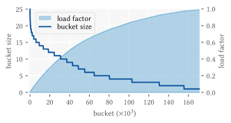
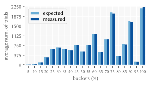
Figure 1. Bucket size and load factor, for $n=10^{6}$ keys and $c=3.5$.

Figure 2. Average number of trials as buckets are processed with a step of 5%, for $n=10^{6}$ keys and $c=3.5$.

Formula (4) shows that pilots $k_{i}$ are quite small, on average. In fact, $\alpha(i)$ will be very small for the first processed buckets, hence yielding small $k_{i}$s. On the other hand, the ordering of buckets by falling size plays a crucial role in keeping $k_{i}$s small even for high load factors. In fact, since the $n$ keys are divided into $m=\lceil cn/\log_{2}n\rceil$ non-uniform buckets, $|B_{i}|$ is a small quantity between 0 and something larger than the average load $n/m$ i.e., $0\leq|B_{i}|\leq\Theta(\frac{\log n}{c})$. Figure 2 shows a pictorial example of such falling distribution of bucket size, for $n=10^{6}$ and $c=3.5$, with growing load factor as buckets are processed by the search.

We argue that Formula (4) gives accurate estimates of the average value of $k_{i}$, hence of the average number of trials needed by the search. Figure 2 shows the average number of trials, both measured and expected using Formula (4), for $n=10^{6}$ keys and $c=3.5$. As evident, the expectation is almost perfectly equal to the measured value for all buckets. The second important thing to note is that while the number of trials tends to increase as buckets are processed for the growing load factor, it can still be very small as it happens, for example, in correspondence of 65%, 80% or 95%. This is a consequence of the small exponent $|B_{i}|$ in the formula.

Directly from Formula (4), we obtain the following result which relates the performance of the search with the parameter $c$.

Theorem 1.

The expected time of the search, for $n$ keys and a parameter $c>\log_{2}e$, is $\mathcal{O}\big{(}n^{1+\Theta(1/c)}\big{)}.$

(Proof omitted due to space constraints.)

Table 1. Empirical entropy of $P$ for $n=10^{6}$ keys, by varying $c$.

$c\rightarrow$	2.5	3.0	3.5	4.0	4.5	5.0	5.5	6.0	6.5	7.0
FCH	16.69	16.85	16.93	16.93	16.87	16.77	16.65	16.49	16.32	16.14
PTHash	13.42	11.68	10.32	9.29	8.48	7.82	7.27	6.82	6.45	6.11

Table 2. Empirical entropy of the front and back parts of $P$ for $n=10^{6}$ keys, by varying $c$.

$c\rightarrow$	2.5	3.0	3.5	4.0	4.5	5.0	5.5	6.0	6.5	7.0
front	3.89	3.51	3.21	2.95	2.77	2.62	2.48	2.38	2.30	2.25
back	10.10	8.87	7.88	7.12	6.51	6.01	5.60	5.25	4.96	4.69

4.2. Front-Back Compression

The net effect of Formula (4) is that $P$ has a low entropy. We report the 0-th order empirical entropy of $P$ in Table 1, for different values of $c$. Specifically, we compare the entropy of $P$ when it stores the pilots determined by our approach and when it stores the displacements following the original FCH procedure. As expected, the entropy of the pilots is smaller than that of the displacements, and actually becomes much smaller for increasing $c$. This clearly suggests that the output of the search can be compressed very well. We now make one step further.

We already noticed that the average number of trials is particularly small for the first processed buckets because of the low load factor. This is graphically evident from Figure 2 looking at the first, say, 30% of the buckets. In other words, the first processed buckets have small pilots. Now we argue that such buckets are those corresponding to the first $p_{2}=0.3m$ entries of $P$ and hold $p1=0.6n$ keys. This is a direct consequence of the skewed distribution of keys into buckets and the order of processing the buckets. Therefore, the front part of $P$, $P[0..p_{2}-1]$, has a lower entropy compared to its back part, $P[p_{2}..m-1]$.

Table 2 shows the entropy of the arrays front and back by varying $c$ and for $n=10^{6}$. As evident, the entropy of the front part is much smaller than that of the back part (by more than $2\times$ on average). This has two immediate consequences. The first, now obvious, is that the array front is more compressible than back, and this saves space compared to the case where $P$ is not partitioned. Note that this partitioning strategy is guaranteed to improve compression by virtue of the skewed distribution, and it is different than partitioning $P$ arbitrarily. The second, even more important, is that we can use two different encoding schemes for front and back to help maintaining good lookup performance and save space. In fact, since front holds 60% of the keys and its size is 30% of $|P|$, it is convenient to use a more time-efficient encoding for front, which is also more compressible, and a more space-efficient encoding for back.

With $P$ rendered as the two partitions front and back, evaluating $f(x)$ is still simple.

1 $f$($x$) :

2       $i=\mbox{\emph{bucket}}(x)$

3       if $i<p_{2}$ then $k_{i}=\mbox{\emph{front}}[i]$

4       else $k_{i}=\mbox{\emph{back}}[i-p_{2}]$

5       return $\mbox{\emph{position}}(x,k_{i})$

6

We then expect the evaluation time of $f(x)$ to be approximately $(p_{1}/n)t_{f}+(1-p_{1}/n)t_{b}$ if $x$ is chosen at random from $S$, with $t_{f}$ and $t_{b}$ being the access time of front and back respectively. In conclusion, because of the values assigned to $p_{1}$ and $p_{2}$, this partitioning strategy allows us to achieve a trade-off between space and lookup time depending on what pair of compressors is used to encode front and back. We will explore this trade-off in Section 5.

4.3. Encoding

Now that we have achieved the first of the two goals mentioned at the beginning of Section 4, i.e., designing an algorithm that guarantees a compressible output, we turn our attention to the second one: devise an encoding scheme that not only takes advantage of the low entropy of $P$ but also maintains noticeable lookup performance.

For simplicity of exposition, let us now focus on the case where $P$ is not partitioned into its front and back parts (the generalization is straightforward). Since $P$ has a low entropy, we argue that a dictionary-based encoding is a good match for our purpose: we collect the distinct values of $P$ into an array $D$, the dictionary, and represent $P$ as an array of references to $D$’s entries. Let $r$ be the size of $D$. As $r$ is smaller than or equal to the number of buckets $m$, which in turn is smaller than the number of keys $n$, we can represent each entry of $P$ using $\lceil\log_{2}r\rceil$ bits instead of the $(\lceil\log_{2}n\rceil+1)$ bits used by FCH. The total space usage is given by the encoded $P$, taking $m\lceil\log_{2}r\rceil$ bits, plus the space of the dictionary $D$. The latter cost is small compared to that of $P$. In particular, the larger $c$ is, the smaller this cost becomes.

The encoding time is linear in the size of $P$, i.e., $\Theta(m)$, thus it takes a small fraction of the total construction. In particular, all encoding methods we consider in Section 5 take linear time.

Using the dictionary, the algorithm for $f(x)$ is as follows.

1 $f$($x$) :

2       $i=\mbox{\emph{bucket}}(x)$

3       $k_{i}=D[P[i]]$

4       return $\mbox{\emph{position}}(x,k_{i})$

5

Compared to FCH, note that we are performing two memory accesses (for $P$ and $D$) instead of one. However, since $D$ is small, its access is likely to be directed to the cache memory of the target machine, e.g., L2 or even L1. Therefore, the indirection only slightly affects lookup performance, as we are going to show in Section 5.

Generalizing the approach to the front and back parts of $P$ is straightforward: each part has its own dictionary and each access to those arrays is executed as shown in step 3 of the pseudocode.

Other more sophisticated options are possible to compress $P$, e.g., Elias-Fano (Elias, 1974; Fano, 1971), or the Simple Dense Coding (SDC) by Fredriksson and Nikitin (2007). As we are going to see in Section 5, using these mechanisms is expected to provide superior compression effectiveness at the price of a slower lookup time.

So far we have explored the effects of the search strategy on compression effectiveness because, as introduced at the beginning of Section 4, a compressible output enables the use of a larger $c$ value that speed up the construction. Let us recall the concrete example made at the end of Section 3: for $n=10^{8}$ 64-bit keys and $c=3$, FCH finds a MPHF in 1 hour and 10 minutes (refer to Section 5 for a description of our experimental setup). PTHash with $c=5.6$ and the introduced front-back encoding finds a MPHF consuming the same amount of space, i.e., 3.0 bits/key. However, it does so in 70 seconds, i.e., $60\times$ faster than FCH. We will present larger and more detailed experiments in Section 5.

4.4. Limiting the Load Factor

Now, we take a deeper look at searching time. According to Formula (4), the searching time is skewed towards the end of the search, because the expected number of trials rapidly grows as $\alpha\rightarrow 1$. This phenomenon is even more evident when using large values of $c$ because a large $c$ lowers the expected number of trials for most of the buckets by lowering the exponent $|B_{i}|$ in Formula (4). In particular, for larger $c$, a small fraction of time is spent on most of the keys, and a large fraction is spent on the last buckets containing only few keys — the heavy “tail” of the distribution.

Figure 3 shows an example of such distribution for $n=10^{9}$ keys and $c=9$. Note the high skewness towards the end, after 85% of the processed buckets: more than 40% of the total search time is spent for only 1.4% of the keys falling into the last 5% of the non-empty buckets.

To avoid the burden of the heavy tail, we search for $f$ in a larger space, say $[n^{\prime}=n/\alpha]$ for a chosen maximum load factor $0<\alpha\leq 1$. For example, if $\alpha=0.99$, then 1% extra space is used to search for $f$. Limiting the maximum achievable load factor clearly lowers searching time, as well as it affects compression effectiveness, by noting that $\mathbb{E}[k_{i}]$ decreases as per Formula (4). In fact, considering a generic $0<\alpha\leq 1$, we obtain the following more general result, whose proof is omitted due to space constraints.

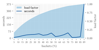
Figure 3. Search time spent as buckets are processed for $n=10^{9}$ keys and $c=9$. The last 11% of the buckets are empty.

Theorem 2.

The expected time of the search, for $n$ keys and parameters $c>\log_{2}e$ and $0<\alpha\leq 1$, is $\mathcal{O}\big{(}n^{1+\Theta(\alpha/c)}\big{)}.$

Now, the issue with searching in a space of size $n^{\prime}=n/\alpha>n$ is that the output of $f$ must be guaranteed to be minimal, i.e., a value in $[n]$, not in $[n^{\prime}]$. One can view the strategy as $f$ leaving some “holes” in its codomain $[n]$ that must then be filled in some appropriate manner. We proceed as follows. Suppose $L$ is the list of holes up to position $n-1$. There are $|L|$ keys that are actually mapped to positions $p_{i}\geq n$, that can fill such holes. Therefore we materialize an array $\mbox{\emph{free}}[0..n^{\prime}-n-1]$, where

$$\mbox{\emph{free}}[p_{i}-n]=L[i],\text{ for each }i=0,\ldots,|L|-1.$$

Note that the space for the array free is that of a sorted integer sequence of size $n^{\prime}-n$, whose maximum value is less than $n$. Thus it takes small space, especially if compressed with Elias-Fano, i.e., $(n^{\prime}-n)(\lceil\log_{2}\frac{n}{n^{\prime}-n}\rceil+2+o(1))$ bits.

Let us discuss an explanatory example. Suppose $n=9$ and $n^{\prime}=14$. There are $n^{\prime}-n=14-9=5$ holes, say in positions $[0,2,8,9,12]$. $L$ is $[0,2,8]$ (holes up to position $n=9$). Therefore there will be $|L|=3$ keys that are mapped out of the range $[0..8]$, and must be those in positions $[10,11,13]$. Then we assign $\mbox{\emph{free}}[10-9]$ = $L[0]$, $\mbox{\emph{free}}[11-9]$ = $L[1]$, and $\mbox{\emph{free}}[13-9]$ = $L[2]$, yielding a final $\mbox{\emph{free}}[0..4]$ = $[\ast,0,2,\ast,8]$, where ‘$\ast$’ indicates an unassigned value.

With the array free, the algorithm for $f(x)$ is as follows.

1 $f$($x$) :

2       $i=\mbox{\emph{bucket}}(x)$

3       $k_{i}=P[i]$

4       $p=(h(x,s)\oplus h(k_{i},s))\,\textup{mod}{\,n^{\prime}}$

5       if $p<n$ then return $p$

6       else return $\mbox{\emph{free}}[p-n]$

7      

8

The second branch of the conditional (else) will be taken with probability $\approx(1-\alpha)$ for random queries. If $\alpha$ is chosen close to 1.0, e.g., 0.99, the branch will be highly predictable, hence barely affecting lookup performance.

Our approach guarantees that each key out of the codomain $[n]$ is mapped back into position with a single access to an array, free. As we are going to show in Section 5, this is considerably faster than the folklore strategy of filling the array free with all available free positions in $[n^{\prime}]$. In fact, in that case, a successor query must be issued over free for every position $p$ returned in step 4 of the pseudocode.

Lastly, the algorithm is directly applicable to any compressed representation of $P$ that supports random access, e.g., the front-back scheme with dictionary-based encoding we have described in the previous sections.

5. Evaluation

In this section we present a comprehensive experimental evaluation of PTHash. All experiments were carried out on a server machine equipped with Intel i9-9900K cores (@3.60 GHz), 64 GB of RAM DDR3 (@2.66 GHz), and running Linux 5 (64 bits). Each core has two private levels of cache memory: 32 KiB L1 cache (one for instructions and one for data); 256 KiB for L2 cache. A shared L3 cache spans 16,384 KiB. Both construction and lookup algorithms were run on a single core of the processor, with the data residing entirely in internal memory. The implementation of PTHash is written in C++ and available at https://github.com/jermp/pthash. The code was compiled with gcc 9.2.1 with optimizating flags -O3 and -march=native.

Lookup time was measured by looking up every single key in the input, and taking the average time between 5 runs. For construction time, we report the average between 3 runs.

We build MPHFs using random integers as input, which is common practice for benchmarking hashing-based algorithms (Esposito et al., 2020; Limasset et al., 2017; Fan et al., 2014; Graf and Lemire, 2020; Müller et al., 2014), given that the nature of the data is completely irrelevant for the space of the data structures. In our case we generated $n$ 64-bit integers uniformly at random in the interval $[0,2^{64})$. We will also evaluate PTHash on real-world string collections to further confirm our results.

Table 3. Construction time, space, and lookup time of PTHash on $n=10^{9}$ random 64-bit keys, for a range of encoding methods and by varying $c$.

$c$	constr. (secs)	space (bits/key)
		C	C-C	D	D-D	D-EF	EF	SDC
6	2441	6.22	5.14	3.21	2.97	2.33	2.21	2.22
7	1579	7.49	6.09	3.75	3.40	2.52	2.39	2.31
8	1190	7.76	6.31	4.28	3.80	2.67	2.57	2.39
9	1010	9.03	7.22	4.82	4.28	2.94	2.77	2.47
10	941	10.37	8.26	5.35	4.65	3.10	2.98	2.53
11	857	11.04	8.83	5.89	5.12	3.32	3.19	2.60
lookup (ns/key)		36	36	49	48	73	96	165

(a) $\alpha=1.00$

$c$	constr. (secs)	space (bits/key)
		C	C-C	D	D-D	D-EF	EF	SDC
6	1736	2.90	2.84	2.90	2.78	2.31	2.17	2.23
7	1033	3.37	3.23	3.14	3.00	2.44	2.27	2.31
8	749	3.57	3.41	3.30	3.14	2.54	2.39	2.41
9	592	3.70	3.52	3.40	3.31	2.72	2.47	2.47
10	510	4.11	3.91	3.77	3.57	2.80	2.59	2.53
11	450	4.14	3.92	4.14	3.92	2.97	2.67	2.59
lookup (ns/key)		37	37	49	49	75	101	170

(b) $\alpha=0.99$

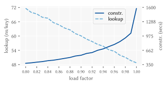
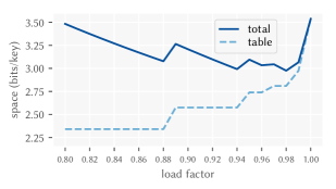
Figure 4. Trade-off between construction time, lookup time, and space of PTHash by varying the load factor, on $n=10^{9}$ random 64-bit keys, $c=7$, and the D-D encoding.

5.1. Tuning

In this section, we are interested in tuning PTHash; we quantify the impact of (i) different encoding schemes to represent the MPHF data structure, (ii) front-back compression, and (iii) varying the load factor.

Compression Effectiveness. In Table 3a we report the performance of PTHash with $\alpha=1.0$ in terms of construction time, lookup time, and bits/key rate, for a range of encoding schemes.

We explain the nomenclature adopted to indicate such encodings. “C” stands for compact and refers to encoding each value in $P$ with $\lceil\log_{2}(\max(P)+1)\rceil$ bits (note that FCH uses this technique, assuming that $\max(P)=n$). “D” indicates the dictionary-based method described in Section 4.3. “EF” stands for Elias-Fano (Elias, 1974; Fano, 1971); “SDC” means Simple Dense Coding (Fredriksson and Nikitin, 2007). Methods indicated with “X-Y” refer to the front-back compression strategy from Section 4.2, where method “X” is used for front and “Y” is used for back.

Table 3a is presented to highlight the spectrum of achievable trade-offs: from top to bottom, we improve construction time by increasing $c$; from left to right we improve space effectiveness but degrade lookup efficiency.

We recall that construction time includes the time of mapping, sorting, searching, and encoding. The most time consuming step is the search, especially for small $c$. For the experiment reported in Table 3, mapping+sorting took 105 seconds, whereas encoding time is essentially the same for all the different methods tested. It ranges from 10 to 15 seconds by varying $c$ from 6 to 11, as $c$ affects the number of buckets used. All the rest of the time is spent during the searching step. Furthermore, we make the following observations.

$\bullet$ Front-back compression pays off for the reasons we explained in Section 4.2, as it always improves space effectiveness, i.e., C-C and D-D are more compact than C and D respectively, while preserving their relative lookup efficiency.

$\bullet$ D and D-D are always more compact than C and C-C, and slightly affect lookup time (+12 ns/key on average for $n=10^{9}$, but smaller for smaller values of $n$), hence confirming that dictionary-based encoding is a good match as explained in Section 4.3.

$\bullet$ EF and SDC are better suited for space effectiveness but also $1.5-3\times$ slower on lookup compared to D-D.

$\bullet$ The configuration D-EF stands in trade-off position between D-D and EF, as the use of EF on the back part improves space but slows down lookup.

Varying the Load Factor. We explained in Section 4.4, that varying $\alpha$ trades off between construction time and lookup efficiency. Figure 4 shows a pictorial example of this trade-off by varying $\alpha$ from 0.80 to 1.00 with step 0.01.

$\bullet$ Construction time decreases significantly, especially in the range $\alpha\in[0.9,1.0]$. In particular, note the sharp decrease when passing from $\alpha=1.0$ to $\alpha=0.99$ as a consequence of avoiding the heavy “tail” already observed in Figure 3.

$\bullet$ Lookup time, instead, increases as $\alpha$ decreases, but at a much slower pace thanks to the fast re-ranking of keys we described in Section 4.4 to guarantee that the output of the function is minimal. In fact, while we are able to obtain a $2\times$ faster construction when passing from, say, $\alpha=1.0$ to $\alpha=0.94$, we only increase lookup time by 6 ns/key. At the other edge of the spectrum visible in Figure 4, if we use $\alpha=0.80$ we obtain a $3\times$ faster construction but also pay $\approx$22 ns/key more on lookup.

$\bullet$ The other relevant advantage is that using a lower load factor does not consume more space but actually even less, for the reasons explained in Section 4.4. In Figure 4 we show the total space of the MPHF and that taken by the pilots table $P$ alone. When $\alpha<1.0$, the total space is given by the space of $P$ plus that of the free array that we compress with Elias-Fano as explained in Section 4.4.

Table 4. The performance of FCH for $n=10^{8}$ random 64-bit keys, and some bits/key rates. For comparison, also the performance of PTHash with $\alpha=0.99$ and encoding C, D-D, and D-EF, is reported.

space (bits/key)		constr. (secs)
		FCH	C		D-D		D-EF
2.50		—	614		173		44
3.00		4286	62	($69\times$)	37	($116\times$)	22	($195\times$)
3.50		985	29	($34\times$)	27	($36\times$)	20	($49\times$)
4.00		463	25	($18\times$)	22	($21\times$)	20	($23\times$)
4.50		340	22	($15\times$)	20	($17\times$)	20	($17\times$)
5.00		145	21	($7\times$)	20	($7\times$)	20	($7\times$)
lookup (ns/key)		30	28		35		55

In Table 3b we report the result of the same experiment in Table 3a but with load factor $\alpha=0.99$. The tables are shown next to each other to better highlight the comparison. As already noted in Figure 4, using just 1% extra space for the search already introduces important advantages, that are observed for any encoding method and any value of $c$: (i) 25–35% reduced construction time; (ii) reduced space usage (with noteworthy improvements for the encodings C and D); (iii) preserved lookup efficiency.

Speeding Up the Search. As a last experiment in this section, Table 4 shows the speed up factors achieved by some PTHash configurations over the construction time of FCH, for the same final bits/key rates. Even using the simple C encoding for PTHash yields $7-69\times$ faster construction with equal (or better) lookup efficiency. Moving to the right-hand side of the table brings further advantages in construction time at the price of a penalty in lookup.

Table 5. Construction time, space, and lookup time for a range of methods on 64-bit random keys.

Method		$n=10^{8}$				$n=10^{9}$
		constr.	space	lookup		constr.	space	lookup
		(secs)	(bits/key)	(ns/key)		(secs)	(bits/key)	(ns/key)
FCH, $c=3$		4286	3.00	30		—	—	—
FCH, $c=4$		463	4.00	30		15904	4.00	35
FCH, $c=5$		145	5.00	30		2937	5.00	35
FCH, $c=6$		81	6.00	30		2133	6.00	35
FCH, $c=7$		68	7.00	30		1221	7.00	35
CHD, $\lambda=4$		121	2.17	204		1972	2.17	419
CHD, $\lambda=5$		358	2.07	204		5964	2.07	417
CHD, $\lambda=6$		1418	2.01	197		23746	2.01	416
EMPHF		24	2.61	147		374	2.61	199
GOV		85	2.23	110		875	2.23	175
BBHash, $\gamma=1$		14	3.06	119		253	3.06	170
BBHash, $\gamma=2$		10	3.71	108		152	3.71	143
BBHash, $\gamma=5$		8	6.87	98		100	6.87	113
RecSplit, $\ell$=5, $b$=5		20	2.95	157		233	2.95	220
RecSplit, $\ell$=8, $b$=100		92	1.80	124		936	1.80	204
RecSplit, $\ell$=12, $b$=9		569	2.23	110		5700	2.23	197
PTHash
(i) C-C, $\alpha$=0.99, $c$=7		42	3.36	28		1042	3.23	37
(ii) D-D, $\alpha$=0.88, $c$=11		19	4.05	46		308	3.94	64
(iii) EF, $\alpha$=0.99, $c$=6		45	2.26	49		1799	2.17	101
(iv) D-D, $\alpha$=0.94, $c$=7		26	3.23	37		689	2.99	55

5.2. Overall Comparison

In this section we compare PTHash with the state-of-the-art techniques reviewed in Section 2.

$\bullet$ FCH (Fox et al., 1992) — It is the only algorithm that we re-implemented (in C++) faithfully to the original paper. We tested the algorithm with $c=3,\ldots,7$ as to almost cover the spectrum of bits/key rates achieved by the other methods.

$\bullet$ CHD (Belazzougui et al., 2009) — We tested the method with parameter $\lambda=4,5,6$. We were unable to use $\lambda=7$ for more than a few thousand keys, as already noted in prior work (Esposito et al., 2020).

$\bullet$ EMPHF (Belazzougui et al., 2014) — It is an efficient implementation of the method based on peeling random hypergraphs. Although the library can also target external memory, we run the algorithm in internal memory.

$\bullet$ GOV (Genuzio et al., 2016, 2020) — It is a method based on solving random linear systems via the Gaussian elimination technique.

$\bullet$ BBHash (Limasset et al., 2017) — It is tested with parameter $\gamma=1,2,5$ as suggested in the original paper. The construction can be multi-threaded, but we used one single thread as to ensure a fair comparison.

$\bullet$ RecSplit (Esposito et al., 2020) — We tested the method using the same configurations used by the authors in their paper, as to offer different trade-offs between construction time and space effectiveness.

For all the above methods we used the source code provided by the original authors (see the References for the corresponding GitHub repositories) and set up a benchmark available at

https://github.com/roberto-trani/mphf_benchmark.

All implementations are in C/C++ except for GOV whose construction is only available in Java.

The results in Table 5 are strongly consistent with those reported in recent previous work (Limasset et al., 2017; Esposito et al., 2020). Out of the many possible configurations for PTHash, we isolate the following four ones.

(i) Optimizing lookup time — C-C encoding, $\alpha=0.99$, $c=7$. PTHash in this configuration achieves the same lookup time as FCH but in much better compressed space. It is similar in space to BBHash with $\gamma=1,2$ but $3-4.5\times$ faster at lookup. Compared to other more space-efficient methods, PTHash is $0.5-1$ bit/key larger but also $5.4-11\times$ faster at lookup.

(ii) Optimizing construction time — D-D encoding, $\alpha=0.88$, $c=11$. This configuration shows that PTHash is competitive in construction time with most of the other techniques, at the price of a larger space consumption. In any case, lookup performance is significantly better, by at least a factor of $2\times$.

(iii) Optimizing space effectiveness — EF encoding, $\alpha=0.99$, $c=6$. In this configuration PTHash achieves a space effectiveness comparable with that of the most succinct methods, i.e., CHD and RecSplit, while still being $2-4\times$ faster at lookup than those methods.

(iv) Optimizing the general trade-off — D-D encoding, $\alpha=0.94$, $c=7$. This configuration tries to achieve a balance between the other three configurations, combining good space effectiveness and construction time, with very fast lookup evaluation.

The evident takeaway message emerging from the comparison in Table 5 is that there is a configuration of PTHash that takes space similar to another method but provides remarkably better lookup performance, with feasible or better construction speed.

5.3. Performance on Variable-Length Keys

In this section, we evaluate PTHash on real-world datasets of variable-length keys. We used natural-language $q$-grams as they are in widespread use in IR, NLP, and machine-learning applications; URLs are interesting as they represent a sort of “worst-case” input given their very long average length. More specifically, we used the 1-grams and 2-grams from the English GoogleBook (version 2) corpus, that are $24,357,349$ and $665,752,080$ in number, respectively. For URLs, we used those of the $\approx$50 million Web pages in the ClueWeb09 (Category B) dataset, and those collected in 2005 from the UbiCrawler (Boldi et al., 2004) relative to the .uk domain, for a total of $49,937,704$ and $39,459,925$ URLs respectively.

While the space of the MPHF data structure is independent from the nature of the data, we choose datasets of increasing average key size to highlight the difference in construction and lookup time compared to fixed-size 64-bit keys. Recall that PTHash hashes each input key only once during construction (to distribute keys into buckets), and once per lookup. Thus, we expect the timings to increase by a constant amount per key, i.e., by the difference between the time to hash a long key and a 64-bit key.

Table 6. Construction time, space, and lookup time of PTHash on some string collections. For comparison, also the performance on 64-bit (fixed-length) random keys is reported. The used PTHash configuration is (iv) — D-D, $\alpha=0.94$, $c=7$.

Collection	avg. key size	constr.	space	lookup
	(bits)	(secs)	(bits/key)	(ns/key)
GoogleBooks 1-grams	82.32	5	3.18	22
64-bit keys	64.00	5	3.18	16
GoogleBooks 2-grams	137.68	430	2.97	63
64-bit keys	64.00	428	2.97	54
ClueWeb09 URLs	437.76	12	3.07	49
64-bit keys	64.00	11	3.07	24
UK2005 URLs	570.96	9	3.11	48
64-bit keys	64.00	9	3.11	22

The performance of PTHash on such variable-length keys is reported in Table 6, under the configuration (iv) — D-D, $\alpha=0.94$, $c=7$. Space effectiveness does not change as expected between real-world datasets and random keys. Construction time does not change either, because of the difference in scale between a process that takes seconds and a hash calculation taking nanoseconds: a constant amount of nanoseconds per key during only the mapping step does not impact. Instead, lookup time grows proportionally to the length of the keys showing that the hash calculation contributes to most of the lookup time of PTHash. More specifically, it increases by $6-9$ ns/key on the $q$-gram datasets, for $1.3-2\times$ longer keys; and by $25-26$ ns/key on URLs, for $7-9\times$ longer keys. These absolute increments show the impact of the hashing of longer keys in a way that is independent of the encoding scheme and size of the dataset.

Concerning the other methods tested in Section 5.2, a similar increase was observed for those hashing the key once per lookup (like PTHash), or much worse for those that hash the key several times per lookup, e.g., BBHash.

6. Conclusions

We presented PTHash, an algorithm that builds minimal perfect hash functions in compact space and retains excellent lookup performance. The result was achieved via a careful revisitation of the framework introduced by Fox, Chen, and Heath (1992) (FCH) in 1992.

We conduct a comprehensive experimental evaluation and show that PTHash takes essentially the same space as that of previous state-of-the art algorithms but provides $2-4\times$ better lookup time. While space effectiveness remains a very important aspect, efficient lookup time is even more important for the minimum perfect hashing problem and its applications. Our C++ implementation is publicly available to encourage the use of PTHash and spur further research on the problem.

Future work will target parallel and external-memory construction, e.g., by splitting the input into chunks and building an independent MPHF on each chunk (Botelho et al., 2013); and devise even more succinct encodings. It would be also interesting to generalize the algorithm to build other types of functions, such as perfect (non-minimal), and $k$-perfect hash functions.

- (1)
- Appleby (2016) Austin Appleby. 2016. SMHasher. https://github.com/aappleby/smhasher.
- Belazzougui et al. (2014) Djamal Belazzougui, Paolo Boldi, Giuseppe Ottaviano, Rossano Venturini, and Sebastiano Vigna. 2014. Cache-oblivious peeling of random hypergraphs. In 2014 Data Compression Conference. IEEE, 352–361. https://github.com/ot/emphf
- Belazzougui et al. (2010) Djamal Belazzougui, Paolo Boldi, Rasmus Pagh, and Sebastiano Vigna. 2010. Fast prefix search in little space, with applications. In European Symposium on Algorithms. Springer, 427–438.
- Belazzougui et al. (2009) Djamal Belazzougui, Fabiano C Botelho, and Martin Dietzfelbinger. 2009. Hash, displace, and compress. In European Symposium on Algorithms. Springer, 682–693. https://github.com/bonitao/cmph
- Belazzougui and Navarro (2014) Djamal Belazzougui and Gonzalo Navarro. 2014. Alphabet-independent compressed text indexing. ACM Transactions on Algorithms (TALG) 10, 4 (2014), 1–19.
- Boldi et al. (2004) Paolo Boldi, Bruno Codenotti, Massimo Santini, and Sebastiano Vigna. 2004. Ubicrawler: A scalable fully distributed web crawler. Software: Practice and Experience 34, 8 (2004), 711–726.
- Botelho et al. (2013) Fabiano C Botelho, Rasmus Pagh, and Nivio Ziviani. 2013. Practical perfect hashing in nearly optimal space. Information Systems 38, 1 (2013), 108–131.
- Broder and Mitzenmacher (2004) Andrei Broder and Michael Mitzenmacher. 2004. Network applications of bloom filters: A survey. Internet mathematics 1, 4 (2004), 485–509.
- Chang and Lin (2005) Chin-Chen Chang and Chih-Yang Lin. 2005. Perfect hashing schemes for mining association rules. Comput. J. 48, 2 (2005), 168–179.
- Chazelle et al. (2004) Bernard Chazelle, Joe Kilian, Ronitt Rubinfeld, and Ayellet Tal. 2004. The Bloomier filter: an efficient data structure for static support lookup tables. In Proceedings of the fifteenth annual ACM-SIAM symposium on Discrete algorithms. Citeseer, 30–39.
- Elias (1974) Peter Elias. 1974. Efficient Storage and Retrieval by Content and Address of Static Files. J. ACM 21, 2 (1974), 246–260.
- Esposito et al. (2020) Emmanuel Esposito, Thomas Mueller Graf, and Sebastiano Vigna. 2020. Recsplit: Minimal perfect hashing via recursive splitting. In 2020 Proceedings of the Twenty-Second Workshop on Algorithm Engineering and Experiments (ALENEX). SIAM, 175–185. https://github.com/vigna/sux
- Fan et al. (2014) Bin Fan, Dave G Andersen, Michael Kaminsky, and Michael D Mitzenmacher. 2014. Cuckoo filter: Practically better than bloom. In Proceedings of the 10th ACM International on Conference on emerging Networking Experiments and Technologies. 75–88.
- Fano (1971) Robert Mario Fano. 1971. On the number of bits required to implement an associative memory. Memorandum 61, Computer Structures Group, MIT (1971).
- Fox et al. (1992) Edward A Fox, Qi Fan Chen, and Lenwood S Heath. 1992. A faster algorithm for constructing minimal perfect hash functions. In Proceedings of the 15th annual international ACM SIGIR conference on Research and development in information retrieval. 266–273.
- Fredman et al. (1984) Michael L Fredman, János Komlós, and Endre Szemerédi. 1984. Storing a sparse table with O(1) worst case access time. Journal of the ACM (JACM) 31, 3 (1984), 538–544.
- Fredriksson and Nikitin (2007) Kimmo Fredriksson and Fedor Nikitin. 2007. Simple compression code supporting random access and fast string matching. In International Workshop on Experimental and Efficient Algorithms. Springer, 203–216.
- Genuzio et al. (2016) Marco Genuzio, Giuseppe Ottaviano, and Sebastiano Vigna. 2016. Fast scalable construction of (minimal perfect hash) functions. In International Symposium on Experimental Algorithms. Springer, 339–352. https://github.com/vigna/Sux4J
- Genuzio et al. (2020) Marco Genuzio, Giuseppe Ottaviano, and Sebastiano Vigna. 2020. Fast scalable construction of ([compressed] static— minimal perfect hash) functions. Information and Computation (2020), 104517.
- Graf and Lemire (2020) Thomas Mueller Graf and Daniel Lemire. 2020. Xor filters: Faster and smaller than bloom and cuckoo filters. Journal of Experimental Algorithmics (JEA) 25 (2020), 1–16.
- Hagerup and Tholey (2001) Torben Hagerup and Torsten Tholey. 2001. Efficient minimal perfect hashing in nearly minimal space. In Annual Symposium on Theoretical Aspects of Computer Science. Springer, 317–326.
- Jacobson (1989) Guy Jacobson. 1989. Space-efficient static trees and graphs. In 30th annual symposium on foundations of computer science. IEEE Computer Society, 549–554.
- Limasset et al. (2017) Antoine Limasset, Guillaume Rizk, Rayan Chikhi, and Pierre Peterlongo. 2017. Fast and scalable minimal perfect hashing for massive key sets. In 16th International Symposium on Experimental Algorithms, Vol. 11. 1–11. https://github.com/rizkg/BBHash
- Lu et al. (2006) Yi Lu, Balaji Prabhakar, and Flavio Bonomi. 2006. Perfect hashing for network applications. In 2006 IEEE International Symposium on Information Theory. IEEE, 2774–2778.
- Majewski et al. (1996) Bohdan S Majewski, Nicholas C Wormald, George Havas, and Zbigniew J Czech. 1996. A family of perfect hashing methods. Comput. J. 39, 6 (1996), 547–554.
- Mehlhorn (1982) Kurt Mehlhorn. 1982. On the program size of perfect and universal hash functions. In 23rd Annual Symposium on Foundations of Computer Science. IEEE, 170–175.
- Müller et al. (2014) Ingo Müller, Peter Sanders, Robert Schulze, and Wei Zhou. 2014. Retrieval and perfect hashing using fingerprinting. In International Symposium on Experimental Algorithms. Springer, 138–149.
- Navarro (2016) Gonzalo Navarro. 2016. Compact data structures: A practical approach. Cambridge University Press.
- Pagh (1999) Rasmus Pagh. 1999. Hash and displace: Efficient evaluation of minimal perfect hash functions. In Workshop on Algorithms and Data Structures. Springer, 49–54.
- Pibiri and Venturini (2017) Giulio Ermanno Pibiri and Rossano Venturini. 2017. Efficient data structures for massive n-gram datasets. In Proceedings of the 40th International ACM SIGIR Conference on Research and Development in Information Retrieval. 615–624.
- Pibiri and Venturini (2019) Giulio Ermanno Pibiri and Rossano Venturini. 2019. Handling Massive N-Gram Datasets Efficiently. ACM Transactions on Information Systems (TOIS) 37, 2 (2019), 25:1–25:41.
- Tarjan and Yao (1979) Robert Endre Tarjan and Andrew Chi-Chih Yao. 1979. Storing a sparse table. Commun. ACM 22, 11 (1979), 606–611.