Towards Corruption-Agnostic Robust Domain Adaptation

Abstract.

Big progress has been achieved in domain adaptation in decades. Existing works are always based on an ideal assumption that testing target domains are i.i.d. with training target domains. However, due to unpredictable corruptions (e.g., noise and blur) in real data like web images, domain adaptation methods are increasingly required to be corruption robust on target domains. In this paper, we investigate a new task, Corruption-agnostic Robust Domain Adaptation (CRDA): to be accurate on original data and robust against unavailable-for-training corruptions on target domains. This task is non-trivial due to large domain discrepancy and unsupervised target domains. We observe that simple combinations of popular methods of domain adaptation and corruption robustness have sub-optimal CRDA results. We propose a new approach based on two technical insights into CRDA: 1) an easy-to-plug module called Domain Discrepancy Generator (DDG) that generates samples that enlarge domain discrepancy to mimic unpredictable corruptions; 2) a simple but effective teacher-student scheme with contrastive loss to enhance the constraints on target domains. Experiments verify that DDG keeps or even improves performance on original data and achieves better corruption robustness than baselines.

1. Introduction

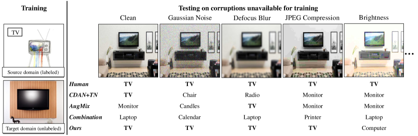
Figure 1. Instances of corruption-agnostic robust domain adaptation (CRDA). To our surprise, existing domain adaptation method (CDAN+TN (Wang et al., 2019)) and corruption robust method (AugMix (Hendrycks et al., 2020b)), even their combination, suffer from unseen corruptions on target domain.

Domain adaptation (DA) (Pan and Yang, 2009) is a promising technique to transfer knowledge from well-labeled source domain to assist unlabeled target domain learning with domain shift. Tremendous efforts on domain adaptation (Li et al., 2020b; Liang et al., 2020; Wang et al., 2019; Long et al., 2018) and domain generalization (DG) (Huang et al., 2020; Matsuura and Harada, 2020; Volpi et al., 2018) indicate the significant progress on domain shift. Besides domain shift, given unpredictable corruptions (e.g., noise and blur) in real data, domain adaptation methods are increasingly required to be corruption robust on target domain (see Fig. 1). However, most DA or DG works only consider transferring source domain knowledge to some specific target datasets, while corruption robustness works (Hendrycks and Dietterich, 2019; Hendrycks et al., 2019a, 2020b; Sun et al., 2020) usually focus on corruptions without domain shift. Thus, there is a question worth considering: how to conduct robustness against unpredictable corruptions in cross domain scenarios?

According to this question, we propose a new task: Corruption-agnostic Robust Domain Adaptation (CRDA), i.e., DA models are required to not only achieve high performance on original target domains, but also be robust against common corruptions that are unavailable for training. Popular DA methods, even combining with existing corruption robustness modules, will get sub-optimal results (see Fig. 1) because they cannot handle well two challenges of CRDA: (1) unpredictable corruptions with large domain discrepancy; (2) weak constraints for robustness on unlabeled target domains. More specifically, previous augmentation robustness methods (Hendrycks et al., 2020b; Zhang et al., 2018a) for corruption-agnostic robustness are always conducted in supervised scenarios with strong classification loss, which may lose effectiveness with domain discrepancy loss on target domains. We first show that after taking into domain information, we can construct more generalized augmentation in cross-domain scenarios. To our knowledge, our work is among the first attempt to unify robustness on domain shift and common corruptions.

To address the above challenges, we propose a novel mechanism towards corruption-agnostic robust domain adaptation called Domain Discrepancy Generator (DDG). Specifically, DDG generates augmentation samples that most enlarge domain discrepancy. Based on several assumptions (detailedly discussed in Section 4.1), these generated samples are proved to be able to represent unpredictable corruptions. Besides, to enhance the constraints on target domains and tackle with unstable features in the early training stage, we propose a teacher-student warm-up scheme via contrastive loss. Specifically, a teacher model is first pre-trained to learn the original representations and then a student model further distills from the teacher model to learn robustness against samlpes generated by DDG via contrastive loss drawn from contrastive learning (Chen et al., 2020a). Our code is available at https://github.com/Mike9674/CRDA.

Our work makes the following contributions:

• We investigate a new scenario called corruption-agnostic robust domain adaptation (CRDA) to equip domain adaptation models with corruption robustness.

• We take use of information of domain discrepancy to propose a novel module Domain Discrepancy Generator (DDG) for corruption robustness that mimic unpredictable corruptions.

• Experiments demonstrate that our method not only significantly improves corruption robustness for DA models but also maintains or even improves classification results on original target domains.

2. Related Work

Table 1. Comparison of related research topics.

Setting	Domain Shift	Target Domain Available	Visual Corruption
Unsupervised Domain Adaptation (Li et al., 2020b; Long et al., 2018; Pan and Yang, 2009)	✓	✓
Domain Generalization (Huang et al., 2020; Matsuura and Harada, 2020; Volpi et al., 2018)	✓
Corruption Robustness (Hendrycks and Dietterich, 2019; Hendrycks et al., 2019a, 2020b; Shorten and Khoshgoftaar, 2019)			✓
Corruption-Agnostic Robust Domain Adaptation	✓	✓	✓

Unsupervised Domain Adaptation.

Tremendous DA methods have made progress in cross-domain applications like recognition (Gopalan et al., 2011), object detection (Chen et al., 2018), and semantic segmentation (Tsai et al., 2018). The core idea is to seek domain-invariant features among source and target domains (Pan and Yang, 2009). A mainstream methodology is distribution alignment, which is mainly based on Maximum Mean Discrepancy (MMD) (Borgwardt et al., 2006; Chen et al., 2019; Li et al., 2020b; Long et al., 2015; Pan et al., 2010) or adversarial methods (Ganin et al., 2016; Goodfellow et al., 2014; Long et al., 2018; Zhang et al., 2018b, 2019). Besides, some works further make improvement by pseudo-labeling (Saito et al., 2017), co-training (Zhang et al., 2018b), entropy regularization (Shu et al., 2018), and evolutionary-based architecture design (Sheng et al., 2021). Recently, increasing researchers focus on more realistic scenarios: considering user privacy, (Li et al., 2020a; Liang et al., 2020) investigate the scenario where only source domain models instead of data available while training. Label corruptions in source domain (Han et al., 2020) is proposed to address the low quality labeling problem in DA. Besides, domain generalization (Huang et al., 2020; Matsuura and Harada, 2020; Volpi et al., 2018) aims to learn domain-invariant representations for unseen target domains. Different from existing literature (see Table 1), we propose a new and realistic topic: corruption-agnostic robust domain adaptation, which investigates corruption robustness in domain adaptation.

Corruption Robustness.

Convolutional networks are proved fragile to simple corruptions by several studies (Dodge and Karam, 2017b; Hosseini et al., 2017). Assuming corruptions are known beforehand, Quality Resilient DNN (Dodge and Karam, 2017a) learns robustness against specific corruptions via a mixture of corruption-specific experts. Instead of knowing testing corruptions beforehand, we propose CRDA to learn general robustness against unseen corruptions. In recent years, increasing works begin to focus on robustness against unseen corruptions. (Vasiljevic et al., 2016) shows that fine-tuning on blurred images fails to generalize to unseen blurs. Several benchmarks (Hendrycks et al., 2020a; Hendrycks and Dietterich, 2019; Hendrycks et al., 2019b; Kang et al., 2019) are constructed to measure generalization to unseen corruptions. Self-supervised learning is found beneficial to corruption robustness (Chen et al., 2020b; Hendrycks et al., 2019a). CutMix (Yun et al., 2019), Mixup (Zhang et al., 2018a), Patch Gaussian (Lopes et al., 2019), Randaugment (Cubuk et al., 2020) and AugMix (Hendrycks et al., 2020b) are under the mainstream that aggregates several general transformations to implicitly represent unseen corruptions. However, current benchmarks and mainstream methods all take it for granted that training and testing data are from the same domain distribution, while CRDA also requires consideration of domain shift, as illustrated in Table 1. Furthermore, instead of aggregating transformations, we propose a new idea that utilize domain discrepancy information to mimic unseen corruptions.

3. Preliminaries

3.1. Problem definition for CRDA

In this paper, we investigate CRDA in the scope of unsupervised domain adaptation for classification. Given labeled source domain $\mathcal{D}_{s}={\{\left(\mathcal{X}_{s},\mathcal{Y}_{s}\right)\}}$, unlabeled target domain $\mathcal{D}_{t}={\{\mathcal{X}_{t}\}}$ ($\mathcal{Y}_{t}$ is unavailable while training), models are required to be robust on corrupted target domain samples $T(\mathcal{X}_{t})$ while maintaining the performance on original target domain, where $T$ denotes a corruption set unavailable for training. Note that $\mathcal{Y}_{s}=\mathcal{Y}_{t}=\{1,\ldots,S\}$ and $P\left(\mathcal{D}_{s}\right)\neq P\left(\mathcal{D}_{t}\right)$.

3.2. Definition of corruption robustness

The concept of corruption robustness is drawn from (Hendrycks and Dietterich, 2019) with slight modification. Given an input sample set $\mathcal{X}$ with the corresponding label set $\mathcal{Y}$, a corruption set $T$ and a model $m=f\circ c$, where $f$ and $c$ respectively denote a feature extractor and a classifier, the corruption robustness is measured by:

(1) $$\mathbb{E}_{t\sim T}\left[\mathbb{P}_{(x,y)\sim(\mathcal{X},\mathcal{Y})}(m(t(x))=y)\right],$$

where we can derive the robustness by aligning features as:

(2) $$\max\left\{\mathbb{E}_{t\sim T}\left[\mathbb{P}_{x\sim\mathcal{X}}(f(t(x))=f(x))\right]\right\}.$$

Here $T$ denotes corruptions derived from (Hendrycks and Dietterich, 2019), which contains 15 kinds of corruptions for $T$ and 5 severities $t$ for each kind (see Fig. 2).

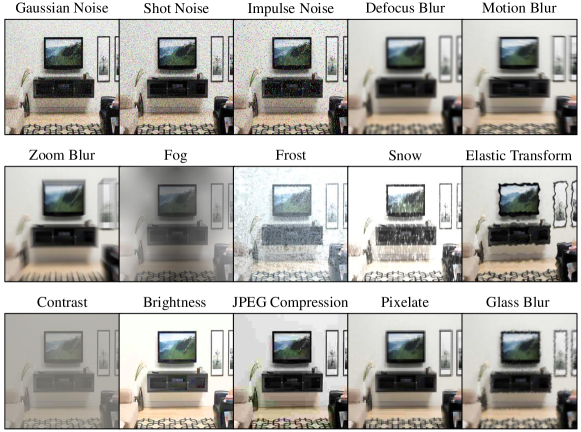
Figure 2. Examples of $15$ kinds of corruptions.

4. Methodology

4.1. Domain Discrepancy Generator

In CRDA setting, the key challenge is that testing corruptions are unavailable during training. Besides, previous data augmentation only encourages networks to memorize the specific corruptions seen during training and leaves models unable to generalize to new corruptions (Geirhos et al., 2018; Vasiljevic et al., 2016). In this section, we attempt to utilize domain information given by domain adaptation to solve this challenge. Thus, Domain Discrepancy Generator (DDG) is proposed to generate samples that most enlarge domain discrepancy to mimic unpredictable corruptions. Fig. 3 illustrated the overall mechanism of DDG. The following is reasonable derivation.

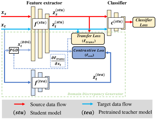
Figure 3. Overall structure of DDG. The yellow part is the classic structure of DA, while the green part is DDG. The gradient of transfer loss is inversely added to the target domain inputs by Projected Gradient Descent (PGD) (Madry et al., 2018) in Algorithm 1 to generate augmentation samples $x_{t}^{(DDG)}$ which is aligned with the original domain-invariant feature extracted by a pretrained teacher model with contrastive loss.

We first assume that corrupted target domain samples hold larger domain discrepancy to source domain than corresponding original target domain samples, which is empirically proved in the supplementary material. Thus, our core idea is to find the points near the original images in sample space that most increase domain discrepancy to represent the most severe corruptions. In domain adaptation, the domain discrepancy is always measured by transfer loss, which is commonly realized by Maximum Mean Discrepancy (MMD) (Borgwardt et al., 2006; Li et al., 2020b; Long et al., 2015; Pan et al., 2010) or adversarial methods (Ganin et al., 2016; Long et al., 2018).

The followings are three basic assumptions for our method, where distance $d_{*}(t(x),x)$ denotes distance between the corrupted images and corresponding original images:

Assumption 1.

The corrupted versions are within the $\delta$-range neighborhood of the original image in sample space ($\boldsymbol{\delta}$ neighborhood for precise) and distance in sample space $d_{s}(t(x),x)$ becomes larger with increase of the severity level of corruption $t$.

Assumption 2.

Within the $\delta$ neighborhood, the severity level $t$ of a corruption $T$ is positively correlated to distance in feature space $d_{f}(f(t(x)),f(x))$.

Assumption 3.

Within the $\delta$ neighborhood, the severity level $t$ of a corruption $T$ is positively correlated to the value of transfer loss $\ell_{trans}(t(x))$.

The empirical proof can be seen in supplementary material. Assumption 2 is drawn from an interesting finding in Section 5.3 that networks always learn order-invariant representations for different severity levels of corruptions.

Based on the above assumptions, we can construct the bridge between domain discrepancy and unpredictable corruptions. Given an input target domain data $x_{t}$, source domain $D_{s}$, transfer loss $\ell_{trans}$ and a corruption set $T$ ($t\in T$) whose corresponding corrupted data $t(x_{t})$ is within the $\delta$ neighborhood of $x_{t}$, DDG generates

(3) $$\begin{split}x_{t}^{(DDG)}&=\mathop{\arg\max}_{\left\|x_{t}^{(DDG)}-x_{t}\right\|\leq\delta}\ell_{trans}\left(f(x_{t}^{(DDG)}),f(D_{s})\right)\\ &\Rightarrow\mathop{\arg\max}_{t\in T}\ell_{trans}\left(f(t\left(x_{t})\right),f(D_{s})\right)=t_{\max}(x_{t}),\end{split}$$

which means the point $x_{t}^{(DDG)}$ near the original target domain sample in sample space that most increases transfer loss (denoting domain discrepancy) can represent the most severe corruption. The proof of Equation (3) can be seen in the supplementary material. In practice, Domain Discrepancy Generator generates such samples via Project Gradient Descent (PGD) (Madry et al., 2018) in Algorithm 1.

Algorithm 1 PGD: Projected Gradient Descent

Input: Target and source doamin data $x_{t},x_{s}$; Feature extractor $f$;Parameters: shift range $\delta$, update stride $\eta$, update step number $n$.

Output: augmented target samples by DDG $x_{t}^{(DDG)}$

1:$i=0$, $x_{t}^{(DDG)}=x_{t}$

2:repeat:

3:    Transfer loss: $\ell=\ell_{trans}(f(x_{t}^{(DDG)}),f(x_{s}))$

4:    Update $x_{t}^{(DDG)}$ by the gradients of transfer loss: $x_{t}^{(DDG)}\leftarrow x_{t}^{(DDG)}+\eta\cdot\text{sign}\left(\frac{\partial{\ell}}{\partial x_{t}^{(DDG)}}\right)$

5:    Clamp $x_{t}^{(DDG)}$ within $\left\|x_{t}^{(DDG)}-x_{t}\right\|\leq\delta$

6:    $i\leftarrow i+1$

7:until $i=n$

8:return $x_{t}^{(DDG)}$

It is worthy noting that the generated samples look similar to adversarial samples (Madry et al., 2018). However, there exists few evidence that domain discrepancy could help corruption robustness in cross domain scenarios like domain adaptation ever before. We first show that it significantly improves corruption robustness on the basis of the bridge between corruptions and domain discrepancy constructed by Equation (3). Meanwhile, DDG works in an unsupervised way while common adversarial training always needs ground-truth labels.

4.2. Overall Learning Framework

The last question is how to learn robustness in unlabeled target domains. Since there is no strong constraints like classification loss in target domains, simply merging samples generated by DDG with the original data may lose the effectiveness. Thus, we utilize contrastive loss (Chen et al., 2020a) to enhance the constraints on target domains. The core idea is simple, i.e., minimizing the feature distance between corrupted samples with their original versions. Besides, to tackle with the unstable features in the early training stage, we further propose a warm-up scheme like teacher-student framework. The teacher model is first trained to extract the original features, while the student model then extracts corrupted features to minimize the distance to corresponding original features. Algorithm 2 shows the overall process of DDG. The proposed contrastive loss is introduced as followed.

Algorithm 2 Overall process for Domain Discrepancy Generator

Input: Data and source labels: $\mathcal{X}_{s}$, $\mathcal{X}_{t}$, $\mathcal{Y}_{s}$; Original DA model $f+c$; Parameters: $\delta=60/255$, $\eta>2\delta$, $n=2$

Output: Robust student model $f^{(stu)}+c^{(stu)}$

1:Train the original model as a teacher model $f^{(tea)}+c^{(tea)}$. Fix the parameters.

2:Construct a student network $f^{(stu)}+c^{(stu)}$ with same structure of $f+c$.

3:repeat:

4:    Draw $x_{s},x_{t},y_{s}$ from $\mathcal{X}_{s},\mathcal{X}_{t},\mathcal{Y}_{s}$.

5:     Generate augmentation samples according to Equation (3) and Algorithm 1: $\qquad x_{t}^{(DDG)}=\text{PGD}\left(x_{t},x_{s},f^{(stu)},\delta,\eta,n\right)$

6:    Update $f^{(stu)}+c^{(stu)}$ according to Equation (10).

7:until Convergence

8:return $f^{(stu)}+c^{(stu)}$

Given a batch of samples ${\{x_{i}\}}_{1}^{N}$, we use feature extractor $f^{(tea)}$ and $f^{(stu)}$ introduced in Algorithm 2 to get $2N$ representation feature vectors:

(4) $$\begin{split}Z^{(tea)}={\left\{z_{i}^{(tea)}|z_{i}^{(tea)}=f^{(tea)}(x_{i})\right\}}_{1}^{N},\\ Z^{(stu)}={\left\{z_{i}^{(stu)}|z_{i}^{(stu)}=f^{(stu)}(x_{i})\right\}}_{1}^{N},\end{split}$$

where we define $Z=Z^{(tea)}\cup Z^{(stu)}={\{z_{i}\}}_{1}^{2N}$. The similarity loss of each two features can be calculated by:

(5) $$\ell_{sim}\left(z_{i},z_{j}\right)=-\log\frac{\exp\left(sim\left(z_{i},z_{j}\right)/\tau\right)}{\sum_{z_{k}\in Z,z_{k}\neq z_{i}}\exp\left(sim\left(z_{i},z_{k}\right)/\tau\right)},$$

where $\tau=0.2$ is a temperature controller to control the similarity extent, and $sim\left(z_{i},z_{j}\right)={z_{i}}^{T}z_{j}/z_{i}z_{j}$ is cosine distance between two vectors. Note that Equation (5) is asymmetric between $z_{i},z_{j}$. The final contrastive loss is defined by:

(6) $$\begin{split}\ell_{con}\left(Z^{(stu)},Z^{(tea)}\right)=\frac{1}{2N}\sum_{i=1}^{N}\left[\ell_{sim}\left(z_{i}^{(stu)},z_{i}^{(tea)}\right)+\ell_{sim}\left(z_{i}^{(tea)},z_{i}^{(stu)}\right)\right],\end{split}$$

where the goal is to minimize the distance between feature representations $z_{i}^{(stu)}$ and $z_{i}^{(tea)}$ of a same sample $x_{i}$. The other kinds of losses defined by the original DA models $\ell_{ori}$, usually containing source domain classification loss $\ell_{cls}$ and transfer loss $\ell_{trans}$in Equation (7), also need to be calculated:

(7) $$\ell_{ori}(x_{s},x_{t},y_{s})=\ell_{cls}(x_{s},y_{s})+\ell_{trans}(x_{s},x_{t}).$$

In fact, contrastive loss does not make $Z^{(stu)}$ definitely same as $Z^{(tea)}$. And thanks to corruptions, the final feature representation $Z^{(stu)}$ has a further distillation on the basis of the teacher model, which may lead to not only improvement on robustness but also better performance on domain invariance.

By utilizing the contrastive loss in Equation (6), we can minimize feature distance between samples $x_{t}^{(DDG)}$ generated by DDG and original samples $x_{t}$ in the target domain iteratively, which leads to features of the most severely corrupted images come closer to original ones, as:

(8) $$\min d_{f}\left(f(x_{t}^{(DDG)}),f(x_{t})\right)\Rightarrow\min d_{f}\left(f(t_{max}(x_{t})),f(x_{t})\right).$$

In practice, Equation (8) is realized by minimizing:

(9) $$\ell_{con}^{(DDG)}\left(x_{t}^{(DDG)},x_{t}\right)=\ell_{con}\left(f^{(stu)}(x_{t}^{(DDG)}),f^{(tea)}(x_{t})\right),$$

Together with the loss defined by the original DA model $\ell_{ori}$ illustrated in Equation (7) and Fig. 3, the final total loss is:

(10) $$\ell_{total}=\ell_{ori}(x_{s},x_{t},y_{s})+\lambda\ell_{con}^{(DDG)}(x_{t}^{(DDG)},x_{t}).$$

Note that DDG only generated samples on target domains and the generated samples are only processed by contrastive loss.

4.3. Further Explanation

Intuitively, DDG should loop many times like $n=10$ in PGD to generates an augmented sample, which is time-consuming. In this section, we theoretically show that we only need to consider the edge point so that by setting $n=2$ is enough, which effectively reduces the time consumption. We begin with the following proposition.

Proposition 1.

Only aligning the edge points $\{x_{t}^{(DDG)}|\|x_{t}^{(DDG)}-x_{t}\|=\delta\}$ around the $\delta$ neighborhood in Equation (3) is enough to gain corruption robustness under the DDG framework.

Given input data $x$, a feature extractor $f$ and a corruption $T$ with continuous severity, we denote the distance in feature space $d_{f}(f(T(x)),f(x))$ as $d(T)$. Then Assumption 2 can be explained as $T$ is positively correlated with $d(T)$. Due to the properties of monotonic function, the upper bound of $d(T)$ is $d(T_{max})$:

(11) $$0\leq d(T)\leq d(T_{max})=d_{max},$$

where $T_{max}$ denotes the most severe level of corruption $T$. By limiting $d_{max}$ to $0$, we get:

(12) $$\lim_{d_{max}\rightarrow 0}{d(T)}=\lim_{d_{max}\rightarrow 0}{d_{f}(f(T(x)),f(x))}=0,$$

which means for all severity levels of corruption $T$, features of corrupted data $T(x)$ and clean data $x$ are the same when $d_{max}\rightarrow 0$. Thus, robustness against a specific corruption is achieved.

Now the last issue is how to limit $d_{max}$ to 0. Note that:

(13) $$d_{max}=d(T_{max})=d_{f}(f(T_{max}(x)),f(x)).$$

Thus, by aligning features of the most severely corrupted samples $T_{max}(x)$ with original features $x$, we get $d_{max}\rightarrow 0$.

Considering Assumption 1, the shift in sample space increases as the increase of the severity level of a corruption $T$. Thus, the most severe corruption $T_{max}(x)$ is always achieved on the edge points of $\delta$ cycle. Then we can use $\{x_{t}^{(DDG)}|\|x_{t}^{(DDG)}-x_{t}\|=\delta\}$ to implicitly represent $T_{max}(x)$ due to the conclusion in Equation (3). By aligning features of these edge points with the original features via minimizing the contrastive loss defined in Equation (9), corruption robustness is achieved under DDG as :

(14) $$\lim_{\ell_{con}^{(DDG)}\rightarrow 0}{d(T)}=\lim_{\ell_{con}^{(DDG)}\rightarrow 0}{d_{f}(f(T(x)),f(x))}=0.$$

Proposition 1 is derived.

Thus, by setting stride $\eta$ bigger than range $2\delta$, we can reach the edge point in one step. In practice, only step $n=2$ gains enough good performance.

4.4. Metrics for corruption robustness

The commonly used standardized aggregate performance measure is the Corruption Error (CE) (Hendrycks and Dietterich, 2019), which can be computed by:

(15) $$\mathrm{CE}_{T}^{f}=\left(\sum_{t=1}^{5}E_{t,T}^{f}\right)\bigg{/}\left(\sum_{t=1}^{5}E_{t,T}^{AlexNet}\right),$$

where $E_{t,T}^{f}$ denotes the error rate of model $f$ on target domain data transformed by corruption $T$ with severity $t$. The $AlexNet$ is trained on clean source domain and tested on corrupted target domain.

The corruption robustness of model $f$ is summarized by averaging Corruption Error values of 15 corruptions introduced in Section 3.2: $\mathrm{CE}_{\text{Gaussian Noise}}^{f},\dots,\mathrm{CE}_{\text{Glass Blur}}^{f}$. The results in the mean CE or mCE (Hendrycks and Dietterich, 2019) for short. mCE is calculated by only one setting (e.g., the Ar:Rw setting in Office-Home). For average performance of corruption robustness on the whole dataset (e.g., Office-Home), we need to average mCE values of all settings.

5. Experiments

5.1. Setups

Datasets.

Office-Home and Office-31 are two benchmark datasets widely adopted for visual domain adaptation algorithms. Experiments are mainly conducted on Office-Home, a relatively challenging dataset. Office-Home (Venkateswara et al., 2017) is a challenging medium sized benchmark, which contains 15588 images from 4 domains (Artistic images (Ar), Clip Art (Cl), Product images (Pr), and Real-World images (Rw)). Each domain consists of 65 object classes under daily life environment. Office-31 (Saenko et al., 2010) is a standard benchmark with 4110 images and 31 classes under office environment. There are totally three domains: Amazon (A), Webcam (W) and DSLR (D).

Corruption.

To check the corruption robust of one given DA model, we create the corrupted version of Office-31 and Office-Home by using the corruption types defined by ImageNet-C (Hendrycks and Dietterich, 2019), a widely used benchmark for corruption robustness. For each image, there exists $15$ corruption types with $5$ levels of severity as illustrated in Fig. 2.

Baselines

To illustrate the improvement on CRDA, we apply our method to CDAN+TN (Long et al., 2018; Wang et al., 2019), a classic baseline model for domain adaptation. We further apply our method to a SOTA DA model DCAN (Li et al., 2020b). Note that the domain discrepancies of CDAN+TN and DCAN are respectively measured by adversarial methods (Goodfellow et al., 2014) and MMD (Borgwardt et al., 2006). We compare our DDG method with AugMix (Hendrycks et al., 2020b), a SOTA method for corruption robustness, which aggregates several general transformations such as contrast, equalization and posterization for data augmentation.

Implementation details

For contrastive loss in Equations (10), the trade-off $\lambda$ is set to $0.5$. For DDG, we conduct Algorithm 2 with $\delta=60/255$, $\eta=6$, $n=2$. Network structures and other hyper-parameters are the same as the original DA models.

Table 2. Accuracy ($\%$) on clean Office-Home data (ResNet-50).

Method	Ar$\to$Cl	Ar$\to$Pr	Ar$\to$Rw	Cl$\to$Ar	Cl$\to$Pr	Cl$\to$Rw	Pr$\to$Ar	Pr$\to$Cl	Pr$\to$Rw	Rw$\to$Ar	Rw$\to$Cl	Rw$\to$Pr	Avg ($\uparrow$)
ResNet	34.9	50.0	58.0	37.4	41.9	46.2	38.5	31.2	60.4	53.9	41.2	59.9	46.1
DAN	43.6	57.0	67.9	45.8	56.5	60.4	44.0	43.6	67.7	63.1	51.5	74.3	56.3
DANN	45.6	59.3	70.1	47.0	58.5	60.9	46.1	43.7	68.5	63.2	51.8	76.8	57.6
JAN	45.9	61.2	68.9	50.4	59.7	61.0	45.8	43.4	70.3	63.9	52.4	76.8	58.3
DWT	50.3	72.1	77.0	59.6	69.3	70.2	58.3	48.1	77.3	69.3	53.6	82.0	65.6
CDAN	50.7	70.6	76.0	57.6	70.0	70.0	57.4	50.9	77.3	70.9	56.7	81.6	65.8
TADA	53.1	72.3	77.2	59.1	71.2	72.1	59.7	53.1	78.4	72.4	60.0	82.9	67.6
SymNets	47.7	72.9	78.5	64.2	71.3	74.2	64.2	48.8	79.5	74.5	52.6	82.7	67.6
MDD	54.9	73.7	77.8	60.0	71.4	71.8	61.2	53.6	78.1	72.5	60.2	82.3	68.1
CDAN+TN	54.1	70.3	77.9	62.2	74.4	73.7	62.4	53.1	81.0	72.8	56.9	82.5	68.4
+AugMix	50.5	70.1	74.9	56.7	69.6	68.7	53.9	50.4	75.9	67.9	58.2	80.6	64.8
+DDG	57.1	74.4	79.4	63.5	75.9	75.3	63.2	54.9	81.9	73.1	58.8	84.2	70.1
DCAN	57.8	76.3	82.9	68.5	72.7	76.7	68.0	56.5	82.1	73.5	60.8	83.3	71.6
+AugMix	55.8	74.8	82.5	67.6	72.1	76.1	67.5	55.0	82.5	73.4	59.0	82.5	70.7
+DDG	58.1	75.2	82.9	68.7	75.0	77.6	68.1	56.6	81.8	73.9	60.6	83.1	71.8

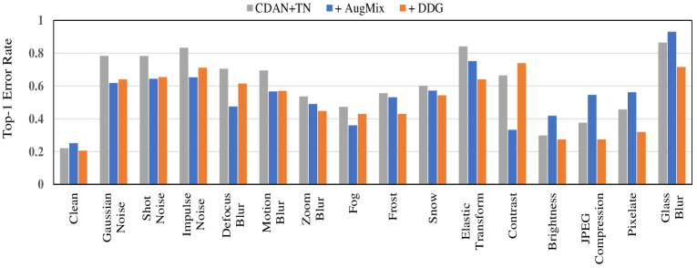
Figure 4. Error rate ($\%$) on Ar$\to$Rw of Office-Home for different corruptions with the most severe level under CRDA (ResNet-50).

5.2. Experiments in CRDA

We compare DDG with AugMix and the original DA models on both corruption robustness and original performance. In addition, we further set an empirical lower bound for CRDA calculated by simply replacing DDG-generated samples in Algorithm 2 with corresponding corrupted samples,which means models that reach the lower bound can be robust against unpredictable corruptions as if they are already known beforehand.

Fig. 4 shows the error rate on clean data and 15 different corruptions with the most severe severity in a single setting. It is reported that DDG achieves improvement over most kinds of corruptions with about 10 percentages in average than the original model and 3 percentages than AugMix. We observe that AugMix only achieves relatively high robustness on several corruptions such as Fog and Contrast. The reason possibly is that these corruptions can be implied by the aggregation of the general transformations defined by AugMix, however, corruptions like Pixelate may lie out of the implied set. Instead, our DDG achieves a much more generalizable implied set thanks to reasonable utilization of domain discrepancy information. It is worthy of noting that DDG can also improve the original accuracy, which is detailedly reported in Table 2.

Table 3. mCE ($\%$) on all cross-domain settings of Office-Home dataset under CRDA (ResNet-50).

Settings	CDAN+TN			DCAN			Lower
	-	AugMix	Ours	-	AugMix	Ours	Bound
Ar$\to$Cl	69.7	69.3	59.8	61.4	63.2	58.3	52.2
Ar$\to$Pr	62.2	52.8	52.2	51.0	49.3	48.0	37.7
Ar$\to$Rw	59.2	56.0	48.0	47.9	46.0	44.6	30.8
Cl$\to$Ar	65.4	73.7	66.0	58.6	57.4	55.2	45.8
Cl$\to$Pr	58.7	56.6	51.9	58.0	57.3	51.6	34.6
Cl$\to$Rw	57.6	61.3	56.2	52.0	53.8	47.5	34.7
Pr$\to$Ar	65.5	72.2	63.6	61.1	58.9	55.1	44.7
Pr$\to$Cl	70.9	71.4	63.6	66.2	65.3	62.2	54.9
Pr$\to$Rw	55.0	55.3	48.8	53.7	48.5	49.4	25.7
Rw$\to$Ar	63.2	62.4	57.8	63.0	59.2	57.7	36.0
Rw$\to$Cl	70.4	61.4	64.4	64.0	64.2	59.9	52.9
Rw$\to$Pr	60.9	52.6	47.9	58.4	52.5	52.6	26.8
Avg ($\downarrow$)	63.2	62.1	56.7	57.9	56.3	53.5	39.7

Table 4. mCE ($\%$) on all cross-domain settings of Office-31 dataset under CRDA (ResNet-50).

Settings	CDAN+TN			DCAN			Lower
	-	AugMix	Ours	-	AugMix	Ours	Bound
A$\to$D	60.3	46.0	48.9	42.3	40.5	36.9	12.3
A$\to$W	59.6	65.2	46.9	40.0	32.4	28.6	10.1
D$\to$A	64.1	66.0	62.4	50.3	53.0	46.6	33.8
D$\to$W	83.5	59.9	69.7	45.2	48.1	35.9	4.6
W$\to$A	64.7	67.9	60.1	60.1	59.8	55.0	36.4
W$\to$D	120.2	64.3	70.9	46.6	54.6	44.5	0.7
Avg ($\downarrow$)	75.4	61.6	59.8	47.4	48.1	41.3	16.3

Fig. 4 also shows that DDG gains no improvement over the Contrast corruption. We argue the reason probably is that this corruption conducts too much shift in sample space which goes beyond the scope of Assumption 1. Possible solutions include loosening the constraint in Assumption 1 and considering the invariant order of pixel values (Contrast does not change the order of pixel values). We leave them for future work.

We report the overall robustness under the whole Office-Home and Office-31 datasets in Table 3 and Table 4 with the standard robustness metric mCE. Results show that even the SOTA model AugMix has sub-optimal results or even worse performance in some settings, which indicates the challenge of CRDA. Despite the challenging task, DDG still gains improvement with obvious margins. Meanwhile, there is still a long way for further study to reach the lower bound in CRDA. Besides robustness, DDG also maintains or improves the original accuracy of DA models. Results are shown in Table 2.

5.3. Empirical analysis

Ablation.

Table 5. mCE ($\%$) on Ar$\to$Rw for different updata strides $\eta$ in DDG

$\delta$	$\eta$	$n$	mCE ($\downarrow$)
$60/255$	$>2\delta$	2	48.0
$60/255$	$>2\delta$	10	49.6
$60/255$	$15/255$	10	51.6
$60/255$	$6/255$	10	52.8

In Section 4.3, we theoretically show only considering the edge points on the $\delta$ cycle is enough for DDG, which is realized by setting stride $\eta>2\delta$ in Algorithm 2. Table 5 reports the mCE under CRDA with different strides $\eta$. Results show that the setting $\eta>2\delta$, which results in only considering the edge points, gains best performance. We conclude the reason why settings $\eta\ll\delta$ perform relatively poorer is that they may wander in the $\delta$ cycle instead of reaching the large-shift points on the edge, which causes a lack of consideration on large-shift corruptions like contrast and blurs. Table 5 also shows that only 2 update steps is enough for DDG to gain corruption robustness. More ablation results can be seen in Appendix.

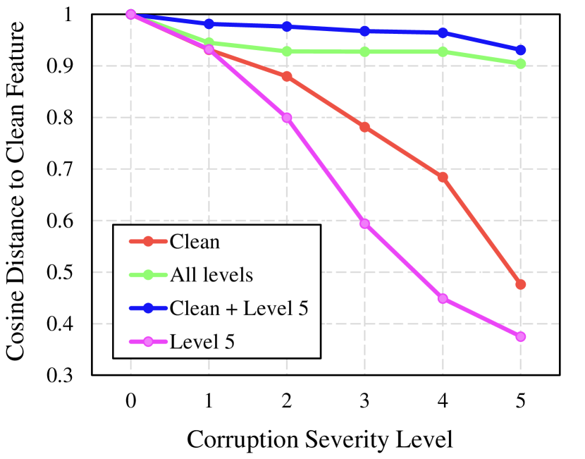
(a) Cosine distance ($\uparrow$)

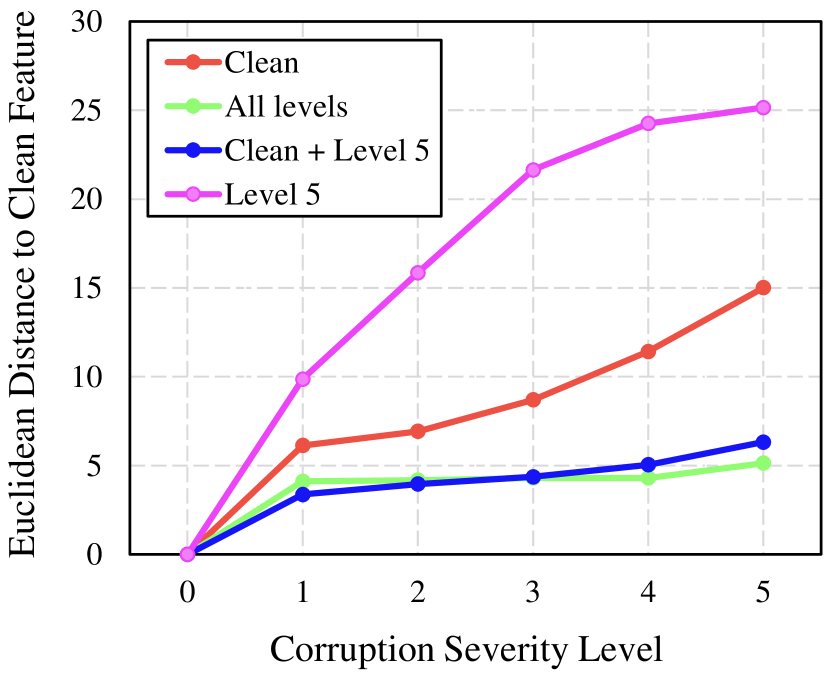
(b) Euclidean distance ($\downarrow$)

Figure 5. Feature distance between a clean image and the versions corrupted by five severity levels of Gaussian Noise on the basis of different models: Clean (a ResNet-50 trained on clean data), All levels (trained on all severity levels of Gaussian Noise), Clean + Level 5 (trained on clean data and severity level 5 Gaussian Noise), Level 5 (trained on data only corrupted by severity level 5).

Teacher-student warm-up scheme.

In this section, we aim to evaluate the effectiveness of the teacher-student warm-up scheme. To compare with simply augmenting samples with testing corruptions, we replace DDG-generated samples in Algorithm 2 with corresponding testing corruptions. Table 6 precisely reports the error rate on original data and corruptions with the most severe severity. Results show that our warm-up scheme can significantly improve the model’s robustness against a specific corruption. Furthermore, our scheme can further improves the model’s original performance instead of negative effect brought by pure data augmentation. In another word, the teacher-student warm-up scheme does not conduct trade-off over robustness and accuracy.

Table 6. Error rate ($\%$) under a specific known corruption on the Ar$\to$Rw setting of Office-Home dataset for teacher-student warm-up shceme.

Corruption	CDAN+TN			Corruption	CDAN+TN
	-	DataAug	Ours		-	DataAug	Ours
Clean	22.1	24.6	21.2	Frost	55.7	30.6	25.5
Gaussian Noise	78.4	33.4	27.8	Snow	60.0	31.2	23.9
Shot Noise	78.3	34.9	26.9	Elastic Transform	84.2	30.0	23.3
Impulse Noise	83.4	33.4	24.4	Contrast	66.4	24.6	23.0
Defocus Blur	70.4	34.9	26.7	Brightness	29.7	26.5	23.6
Motion Blur	69.5	28.4	24.3	JPEG Compression	37.6	29.0	23.2
Zoom Blur	53.6	29.4	23.1	Pixelate	45.7	26.9	22.6
Fog	47.3	24.6	23.6	Glass Blur	86.4	37.0	27.8

Order-invariant representations of corruptions.

We empirically observe that the distance between the corrupted versions and the corresponding clean image in feature space (feature distance for precise) is always positively correlated to the severity of corruptions. Training details are shown in the supplementary material. Fig. 5 shows that even only trained on clean and corrupted samples with a single severity (Clean + Level 5), models still learn the positive correlation instead of relatively nearer feature distance on a specific severity. In a word, networks always learn order-invariant representations in feature space for different levels of severity, which contributes to Assumption 2 in Section 4.1.

6. Conclusion

In this paper, we throw a new sight to domain adaptation to investigate a more realistic new task, Corruption-agnostic Robust Domain Adaptation (CRDA). Taking domain information into consideration, we present a new idea for corruption robustness called Domain Discrepancy Generator (DDG) that mimic unpredictable corruptions via generating samples most enlarging domain discrepancy. Besides, we propose a teacher-student warm-up scheme via contrastive loss to enhance the constraints on unlabelled target domains and stabilize the early training stage feature. Empirical results justify that DDG outperforms existing baselines on original accuracy and achieves better corruption robustness.

References

- (1)
- Borgwardt et al. (2006) Karsten M Borgwardt, Arthur Gretton, Malte J Rasch, Hans-Peter Kriegel, Bernhard Schölkopf, and Alex J Smola. 2006. Integrating structured biological data by kernel maximum mean discrepancy. Bioinformatics 22, 14 (2006), e49–e57.
- Chen et al. (2019) Chao Chen, Zhihong Chen, Boyuan Jiang, and Xinyu Jin. 2019. Joint domain alignment and discriminative feature learning for unsupervised deep domain adaptation. In Proceedings of the AAAI Conference on Artificial Intelligence, Vol. 33. 3296–3303.
- Chen et al. (2020a) Ting Chen, Simon Kornblith, Mohammad Norouzi, and Geoffrey Hinton. 2020a. A simple framework for contrastive learning of visual representations. In ICML.
- Chen et al. (2020b) Tianlong Chen, Sijia Liu, Shiyu Chang, Yu Cheng, Lisa Amini, and Zhangyang Wang. 2020b. Adversarial Robustness: From Self-Supervised Pre-Training to Fine-Tuning. In Proceedings of the IEEE/CVF Conference on Computer Vision and Pattern Recognition. 699–708.
- Chen et al. (2018) Yuhua Chen, Wen Li, Christos Sakaridis, Dengxin Dai, and Luc Van Gool. 2018. Domain adaptive faster r-cnn for object detection in the wild. In Proceedings of the IEEE conference on computer vision and pattern recognition. 3339–3348.
- Cubuk et al. (2020) Ekin D Cubuk, Barret Zoph, Jonathon Shlens, and Quoc V Le. 2020. Randaugment: Practical automated data augmentation with a reduced search space. In Proceedings of the IEEE/CVF Conference on Computer Vision and Pattern Recognition Workshops. 702–703.
- Dodge and Karam (2017a) Samuel Dodge and Lina Karam. 2017a. Quality resilient deep neural networks. arXiv preprint arXiv:1703.08119 (2017).
- Dodge and Karam (2017b) Samuel Dodge and Lina Karam. 2017b. A study and comparison of human and deep learning recognition performance under visual distortions. In 2017 26th international conference on computer communication and networks (ICCCN). IEEE, 1–7.
- Ganin et al. (2016) Yaroslav Ganin, Evgeniya Ustinova, Hana Ajakan, Pascal Germain, Hugo Larochelle, François Laviolette, Mario Marchand, and Victor Lempitsky. 2016. Domain-adversarial training of neural networks. The Journal of Machine Learning Research 17, 1 (2016), 2096–2030.
- Geirhos et al. (2018) Robert Geirhos, Carlos RM Temme, Jonas Rauber, Heiko H Schütt, Matthias Bethge, and Felix A Wichmann. 2018. Generalisation in humans and deep neural networks. In Advances in neural information processing systems. 7538–7550.
- Goodfellow et al. (2014) Ian Goodfellow, Jean Pouget-Abadie, Mehdi Mirza, Bing Xu, David Warde-Farley, Sherjil Ozair, Aaron Courville, and Yoshua Bengio. 2014. Generative adversarial nets. In Advances in Neural Information Processing Systems (NIPS). 2672–2680.
- Gopalan et al. (2011) Raghuraman Gopalan, Ruonan Li, and Rama Chellappa. 2011. Domain adaptation for object recognition: An unsupervised approach. In 2011 international conference on computer vision. IEEE, 999–1006.
- Han et al. (2020) Zhongyi Han, Xian-Jin Gui, Chaoran Cui, and Yilong Yin. 2020. Towards Accurate and Robust Domain Adaptation under Noisy Environments. In Proceedings of the Twenty-Ninth International Joint Conference on Artificial Intelligence, IJCAI-20, Christian Bessiere (Ed.). IJCAI, 2269–2276. Main track.
- Hendrycks et al. (2020a) Dan Hendrycks, Steven Basart, Norman Mu, Saurav Kadavath, Frank Wang, Evan Dorundo, Rahul Desai, Tyler Zhu, Samyak Parajuli, Mike Guo, Dawn Song, Jacob Steinhardt, and Justin Gilmer. 2020a. The Many Faces of Robustness: A Critical Analysis of Out-of-Distribution Generalization. arXiv preprint arXiv:2006.16241 (2020).
- Hendrycks and Dietterich (2019) Dan Hendrycks and Thomas Dietterich. 2019. Benchmarking neural network robustness to common corruptions and perturbations. In ICLR.
- Hendrycks et al. (2019a) Dan Hendrycks, Mantas Mazeika, Saurav Kadavath, and Dawn Song. 2019a. Using self-supervised learning can improve model robustness and uncertainty. In Advances in Neural Information Processing Systems. 15663–15674.
- Hendrycks et al. (2020b) Dan Hendrycks, Norman Mu, Ekin D Cubuk, Barret Zoph, Justin Gilmer, and Balaji Lakshminarayanan. 2020b. Augmix: A simple data processing method to improve robustness and uncertainty. In Augmix: A simple data processing method to improve robustness and uncertainty (ICLR).
- Hendrycks et al. (2019b) Dan Hendrycks, Kevin Zhao, Steven Basart, Jacob Steinhardt, and Dawn Song. 2019b. Natural Adversarial Examples. arXiv preprint arXiv:1907.07174 (2019).
- Hosseini et al. (2017) Hossein Hosseini, Baicen Xiao, and Radha Poovendran. 2017. Google’s cloud vision api is not robust to noise. In 2017 16th IEEE International Conference on Machine Learning and Applications (ICMLA). IEEE, 101–105.
- Huang et al. (2020) Zeyi Huang, Haohan Wang, Eric P. Xing, and Dong Huang. 2020. Self-Challenging Improves Cross-Domain Generalization. In ECCV.
- Kang et al. (2019) Daniel Kang, Yi Sun, Dan Hendrycks, Tom Brown, and Jacob Steinhardt. 2019. Testing robustness against unforeseen adversaries. arXiv preprint arXiv:1908.08016 (2019).
- Li et al. (2020a) Rui Li, Qianfen Jiao, Wenming Cao, Hau-San Wong, and Si Wu. 2020a. Model Adaptation: Unsupervised Domain Adaptation without Source Data. In Proceedings of the IEEE/CVF Conference on Computer Vision and Pattern Recognition. 9641–9650.
- Li et al. (2020b) Shuang Li, Chi Harold Liu, Qiuxia Lin, Binhui Xie, Zhengming Ding, Gao Huang, and Jian Tang. 2020b. Domain Conditioned Adaptation Network. In Thirty-Fourth AAAI Conference on Artificial Intelligence (AAAI-20).
- Liang et al. (2020) Jian Liang, Dapeng Hu, and Jiashi Feng. 2020. Do We Really Need to Access the Source Data? Source Hypothesis Transfer for Unsupervised Domain Adaptation. In International Conference on Machine Learning (ICML). xx–xx.
- Long et al. (2015) Mingsheng Long, Yue Cao, Jianmin Wang, and Michael Jordan. 2015. Learning transferable features with deep adaptation networks. In International conference on machine learning. PMLR, 97–105.
- Long et al. (2018) Mingsheng Long, Zhangjie Cao, Jianmin Wang, and Michael I Jordan. 2018. Conditional adversarial domain adaptation. In Advances in Neural Information Processing Systems. 1640–1650.
- Lopes et al. (2019) Raphael Gontijo Lopes, Dong Yin, Ben Poole, Justin Gilmer, and Ekin D Cubuk. 2019. Improving robustness without sacrificing accuracy with patch gaussian augmentation. arXiv preprint arXiv:1906.02611 (2019).
- Madry et al. (2018) Aleksander Madry, Aleksandar Makelov, Ludwig Schmidt, Dimitris Tsipras, and Adrian Vladu. 2018. Towards deep learning models resistant to adversarial attacks. In ICLR.
- Matsuura and Harada (2020) Toshihiko Matsuura and Tatsuya Harada. 2020. Domain Generalization Using a Mixture of Multiple Latent Domains. In AAAI.
- Pan et al. (2010) Sinno Jialin Pan, Ivor W Tsang, James T Kwok, and Qiang Yang. 2010. Domain adaptation via transfer component analysis. IEEE Transactions on Neural Networks 22, 2 (2010), 199–210.
- Pan and Yang (2009) Sinno Jialin Pan and Qiang Yang. 2009. A survey on transfer learning. IEEE Transactions on knowledge and data engineering 22, 10 (2009), 1345–1359.
- Saenko et al. (2010) Kate Saenko, Brian Kulis, Mario Fritz, and Trevor Darrell. 2010. Adapting visual category models to new domains. In ECCV.
- Saito et al. (2017) Kuniaki Saito, Yoshitaka Ushiku, and Tatsuya Harada. 2017. Asymmetric tri-training for unsupervised domain adaptation. arXiv preprint arXiv:1702.08400 (2017).
- Sheng et al. (2021) Kekai Sheng, Ke Li, Xiawu Zheng, Jian Liang, Weiming Dong, Feiyue Huang, Rongrong Ji, and Xing Sun. 2021. On Evolving Attention Towards Domain Adaptation. arXiv preprint arXiv:2103.13561 (2021).
- Shorten and Khoshgoftaar (2019) Connor Shorten and Taghi M Khoshgoftaar. 2019. A survey on image data augmentation for deep learning. Journal of Big Data 6, 1 (2019), 60.
- Shu et al. (2018) Rui Shu, Hung H Bui, Hirokazu Narui, and Stefano Ermon. 2018. A dirt-t approach to unsupervised domain adaptation. In ICLR.
- Sun et al. (2020) Yu Sun, Xiaolong Wang, Liu Zhuang, John Miller, Moritz Hardt, and Alexei A. Efros. 2020. Test-Time Training with Self-Supervision for Generalization under Distribution Shifts. In ICML.
- Tsai et al. (2018) Yi-Hsuan Tsai, Wei-Chih Hung, Samuel Schulter, Kihyuk Sohn, Ming-Hsuan Yang, and Manmohan Chandraker. 2018. Learning to adapt structured output space for semantic segmentation. In Proceedings of the IEEE Conference on Computer Vision and Pattern Recognition. 7472–7481.
- Vasiljevic et al. (2016) Igor Vasiljevic, Ayan Chakrabarti, and Gregory Shakhnarovich. 2016. Examining the impact of blur on recognition by convolutional networks. arXiv preprint arXiv:1611.05760 (2016).
- Venkateswara et al. (2017) Hemanth Venkateswara, Jose Eusebio, Shayok Chakraborty, and Sethuraman Panchanathan. 2017. Deep hashing network for unsupervised domain adaptation. In CVPR.
- Volpi et al. (2018) Riccardo Volpi, Hongseok Namkoong, Ozan Sener, John C Duchi, Vittorio Murino, and Silvio Savarese. 2018. Generalizing to unseen domains via adversarial data augmentation. In Advances in neural information processing systems. 5334–5344.
- Wang et al. (2019) Ximei Wang, Ying Jin, Mingsheng Long, Jianmin Wang, and Michael I Jordan. 2019. Transferable normalization: Towards improving transferability of deep neural networks. In Advances in Neural Information Processing Systems. 1953–1963.
- Yun et al. (2019) Sangdoo Yun, Dongyoon Han, Seong Joon Oh, Sanghyuk Chun, Junsuk Choe, and Youngjoon Yoo. 2019. Cutmix: Regularization strategy to train strong classifiers with localizable features. In Proceedings of the IEEE International Conference on Computer Vision. 6023–6032.
- Zhang et al. (2018a) Hongyi Zhang, Moustapha Cisse, Yann N Dauphin, and David Lopez-Paz. 2018a. mixup: Beyond empirical risk minimization. International Conference on Learning Representations (2018).
- Zhang et al. (2018b) Weichen Zhang, Wanli Ouyang, Wen Li, and Dong Xu. 2018b. Collaborative and adversarial network for unsupervised domain adaptation. In Proceedings of the IEEE Conference on Computer Vision and Pattern Recognition. 3801–3809.
- Zhang et al. (2019) Yabin Zhang, Hui Tang, Kui Jia, and Mingkui Tan. 2019. Domain-symmetric networks for adversarial domain adaptation. In Proceedings of the IEEE Conference on Computer Vision and Pattern Recognition. 5031–5040.