Improving Test Distance for Failure Clustering with Hypergraph Modelling

Abstract.

Automated debugging techniques, such as Fault Localisation (FL) or Automated Program Repair (APR), are typically designed under the Single Fault Assumption (SFA). However, in practice, an unknown number of faults can independently cause multiple test case failures, making it difficult to allocate resources for debugging and to use automated debugging techniques. Clustering algorithms have been applied to group the test failures according to their root causes, but their accuracy can often be lacking due to the inherent limits in the distance metrics for test cases. We introduce a new test distance metric based on hypergraphs and evaluate their accuracy using multi-fault benchmarks that we have built on top of Defects4J and SIR. Results show that our technique, Hybiscus, can automatically achieve perfect clustering (i.e., the same number of clusters as the ground truth number of root causes, with all failing tests with the same root cause grouped together) for 418 out of 605 test runs with multiple test failures. Better failure clustering also allows us to separate different root causes and apply FL techniques under SFA, resulting in saving up to 82% of the total wasted effort when compared to the state-of-the-art technique for multiple fault localisation.

1. Introduction

As software systems grow in size and complexity, the cost of debugging has significantly increased. Many automated techniques have been proposed and studied to reduce the burden of debugging. Fault Localisation (FL) aims to automatically identify the location of the root cause of the observed test failure (Wong et al., 2016), using various information such as program spectrum (Jones and Harrold, 2005; Naish et al., 2011; Wong et al., 2013), mutation analysis (Moon et al., 2014; Hong et al., 2017; Papadakis and Le Traon, 2012, 2015), and textual similarity between bug reports and source code (Zhou et al., 2012; Saha et al., 2013; Lukins et al., 2008). Automated Program Repair (APR) uses results of FL to identify the location of the fault, and seeks to generate patches, either by finding ingredients of the patch from existing code (Yuan and Banzhaf, 2018; Wen et al., 2018), or by synthesising the patch based on the observed violation of oracles (Le et al., 2017; Mechtaev et al., 2016).

Most FL and APR techniques that have made significant advances share a common basis, which is the Single Fault Assumption (SFA): they assume that there exists a single fault in the System Under Test (SUT) that is responsible for all observed test failures. SFA allows us to precisely measure the effectiveness of FL and APR techniques, which in turn enables the design of more advanced automated debugging techniques. Fault benchmarks such as Defects4J (Just et al., 2014) contain significant amounts of effort to capture and reproduce real-world faults in isolation, so that automated techniques can be studied and developed under SFA.

In practice, however, SFA does not always hold. It is entirely possible that a set of changes made to SUT contains multiple faults, each being the root cause of different test cases. Multiple faults that occur simultaneously present challenges not only to automated debugging techniques developed under SFA (DiGiuseppe and Jones, 2015; Xue and Namin, 2013; DiGiuseppe and Jones, 2011), but also to human engineers whose very first task is to understand how many faults there are to debug.

Given multiple test failures, how can we decide the number of different root causes, as well as the mapping between the causes and the observed failures? With any SUT of realistic complexity, the number of failing test cases may not directly indicate the number of different root causes, as the dependency structures in SUT can force a single fault to affect the outcomes of multiple test cases. Clustering of test cases has been proposed as a solution to group failing test cases (Jones et al., 2007; Golagha et al., 2017; Gao and Wong, 2017; Golagha et al., 2019), but the accuracy of clustering, in terms of both the number of clusters (i.e., the number of root causes) and the cluster membership (i.e., the mapping between root causes and test failures) can be lacking. Inaccurate clustering would introduce additional challenges to the debugging process, due to inefficient resource management based on incorrect estimation of root causes and the sub-optimal performance of automated debugging techniques.

We propose Hybiscus, a hypergraph based failure representation and clustering technique that can accurately predict both the number of root causes and the mapping between root causes and test failures. Hybiscus introduces a hypergraph representation of test coverage, from which it also derives a novel test distance metric. In addition to Hybiscus, we also introduce multiple-fault variants of widely studied fault benchmarks, Defects4J and SIR: both were constructed by systematically merging real (Defects4J) and seeded (SIR) faults in the original benchmarks. Our empirical evaluation shows that, when used with Agglomerative Hierarchical Clustering (AHC) and a distance-based estimation of cluster numbers, Hybiscus can significantly outperform other failure clustering methods. Once clustered, Hybiscus can apply total wasted effort when compared to the state-of-the-art multi-fault FL technique, MSeer (Gao and Wong, 2017).

The main contribution of this paper includes the following.

• We propose a novel test distance metric, hdist, based on hypergraph modelling. Our hypergraph based distance metric can measure the dissimilarity between two test cases while reflecting their their higher-order relationship with the remainder of the test suite.

• We introduce multiple fault variants of the Defects4J and SIR benchmarks to evaluate our novel test distance metric in the context of failure clustering. Each of the faulty versions in our variants includes up to seven distinct faults. Our datasets for Java and C subjects are publicly available and can be used for future research on automated debugging of multiple faults. To the best of our knowledge, there has been no failure clustering work validated on both Java and C subjects.

• The empirical evaluation using the multiple fault versions of Defects4J and SIR shows that our novel hypergraph-based test distance metric can more accurately measure the distance between test cases when compared to other vector-, set-, and ranking-based metrics in the application on failure clustering.

• We introduce Hybiscus , a failure clustering technique that uses the hypergraph-based test distance. Using heuristic estimation of cluster numbers, Hybiscus can perfectly cluster 69% of the studied multiple fault subjects, i.e., with the correct number of root causes and correct groupings of failing test cases, without any human intervention. Using the results of clustering, Hybiscus can also localise each of the multiple faults saving up to 82% of the total wasted effort when compared to the state-of-the-art multiple fault localisation technique, MSeer.

The paper is structured as follows. Section 2 formally introduces the problem of failure clustering, with a motivating example. Section 3 presents the hypergraph representation of test coverage, as well as the distance metric between test coverage and our clustering formulation. Section 4 describes how multiple fault variants of Defects4J and SIR were constructed and presents our experimental setup. Section 5 presents the results of our empirical evaluation, and Section 6 discusses threats to validity. Section 7 presents related work, and Section 8 concludes.

2. Failure Clustering

Let us consider a program that consists of $M$ components, $C=\{c_{1},c_{2},\ldots,c_{M}\}$, and a test suite with $N$ test cases, $T=\{t_{1},t_{2},\ldots,t_{N}\}$. After executing $T$, let $T_{P}$ and $T_{F}$ be the set of passing and failing test cases, respectively (note that the test coverage can be represented by a $N\times M$ matrix $A$, whose entry $A_{i,j}$ is 1 if $t_{i}$ executes $c_{j}$ and 0 otherwise). When there are multiple failing test cases, i.e., $|T_{F}|>1$, a developer should separate different failures according to their root causes in order to debug them one by one.

The problem of failure clustering is to assign cluster membership to failing test cases in $T_{F}$ so that, in the resulting clusters, $P=\{T_{1},\ldots,T_{k}\}$, failures due to the same root cause are grouped together. For clustering problems for which ground-truth cluster assignment $P_{true}$ is known, there are two desirable properties of a good cluster assignment $P$ (Rosenberg and Hirschberg, 2007):

• Homogeneity: Every member of a cluster in $P$ is assigned to the same cluster in $P_{true}$.

• Completeness: Every member of a cluster in $P_{true}$ is assigned to the same cluster in $P$.

For the failure clustering problem, a perfect cluster assignment is the one that assigns each failing test in $T_{F}$ to groups that share the same root cause: each cluster in $P$ has its own root cause, which is different from those of all other clusters. In this context, we can rephrase homogeneity and completeness as follows:

• All failing test cases in a cluster share the same root cause (homogeneity).

• All failing test cases sharing the same root cause belong to the same cluster (completeness).

If a failure clustering is not homogeneous, anyone using one of the clusters to understand one of the root causes will be misled, as the non-homogeneous test failures will add noise to the process. If a failure clustering is not complete, there will be redundant clusters, which subsequently will increase the inspection workload for the developer. Finding both the correct assignment of failing test cases to root causes and the correct number of root causes is important for effective and efficient debugging of multiple faults.

2.1. A Motivating Example

Let us consider a System Under Test (SUT) with six components, the set of which is denoted by $C=\{c_{1},\ldots,c_{6}\}$. Let $T$ be a test suite with five test cases, $T=\{t_{1},\ldots,t_{5}\}$. Suppose there are two faulty components, $c_{3}$ and $c_{4}$: test case $t_{3}$ fails due to the execution of $c_{3}$, while $t_{4}$ and $t_{5}$ fail due to $c_{4}$. The full execution traces are shown in Table 1. Our goal is to cluster the set of failing test cases, $T_{F}=\{t_{3},t_{4},t_{5}\}$, into $P=\{\{t_{3}\},\{t_{4},t_{5}\}\}$.

Table 1. Example of test execution traces

TC	$t_{1}$	$t_{2}$	$t_{3}$	$t_{4}$	$t_{5}$
Trace	$\{c_{1},c_{2},c_{5},c_{6}\}$	$\{c_{1},c_{2},c_{5},c_{6}\}$	$\{c_{2},\underline{\mathbf{c_{3}}},c_{5}\}$	$\{c_{1},\underline{\mathbf{c_{4}}}\}$	$\{c_{2},\underline{\mathbf{c_{4}}},c_{5}\}$
Result	Pass	Pass	Fail	Fail	Fail

We can expect that failing test cases with similar behaviour are more likely to share the same root cause. Since execution traces reflect test case behaviour, we can cluster failing test cases using a distance metric defined over the execution traces. In the next section, we discuss distance metrics and the test execution trace representations used in the literature to perform failure clustering.

2.2. Distance Metrics for Failure Clustering

Various distance metrics have been proposed for failure clustering to capture the proximity between observed test failures (Liu et al., 2008). The representation of test execution guides the choice of a distance metric, which in turn affects the performance of failure clustering (Zakari et al., 2020). The most widely studied representations of test execution traces are numerical vectors, sets, and fault localisation ranks.

2.2.1. Numerical Vectors

A test execution trace can be represented as a $M$-dimensional vector. When the vector is binary, this representation becomes the coverage vector, 1 meaning the corresponding component being covered, and 0 otherwise. For example, the test case $t_{3}$ in Section 2.1 can be represented by $(0,1,1,0,1,0)$. For binary vector representation, Hamming, Cosine, or Euclidean distance can be used to measure distances between test cases (Yoo et al., 2009; Huang et al., 2013; Wang et al., 2014; Golagha et al., 2017). Beyond binary representation, each vector element could also contain the number of times the corresponding component has been executed. However, to the best of our knowledge, most existing failure clustering literature focuses on binary representation.

While intuitive, previous literature (Gao and Wong, 2017; Liu et al., 2008) argues that this representation is inappropriate for failure clustering, because test cases that fail due to the same root cause may still produce considerably different execution traces. For example, $t_{4}$ and $t_{5}$ in Section 2.1 only share one program component, $c_{4}$, which is the root cause. Using Hamming and Euclidean distance metrics, the distances between the binary vector representations of $t_{3}$, $t_{4}$ and $t_{5}$ are as follows:

• $Hamming(t_{3},t_{4})=0.83$ and $Euclidean(t_{3},t_{4})=2.24$

• $Hamming(t_{4},t_{5})=0.50$ and $Euclidean(t_{4},t_{5})=1.73$

• $Hamming(t_{3},t_{5})=\textbf{0.33}$ and $Euclidean(t_{3},t_{5})=\textbf{1.41}$

According to these results, $t_{3}$ and $t_{5}$ are the closest among all pairs of failing test cases. Consequently, the pair of $t_{3}$ and $t_{5}$ is more likely to be assigned to the same cluster than that of $t_{4}$ and $t_{5}$ by any clustering algorithm that uses these distance metrics. However, this is not aligned with the ground-truth clustering: $\{\{t_{3}\},\{t_{4},t_{5}\}\}$.

2.2.2. Sets

An execution trace can also be represented as a set of all program components it covers. There are many set similarity metrics that are widely used, such as Jaccard or Sørensen-Dice coefficient. However, the set representation can be vulnerable to variance in execution traces of failing tests, such like the vector representation. Consider the set-based distances between failing test cases in the motivating example:

• $Jaccard(t_{3},t_{4})=1.00$ and $Dice(t_{3},t_{4})=1.00$

• $Jaccard(t_{4},t_{5})=0.75$ and $Dice(t_{4},t_{5})=0.66$

• $Jaccard(t_{3},t_{5})=\textbf{0.50}$ and $Dice(t_{3},t_{5})=\textbf{0.33}$

As in the case of the vector representation, the set-based distance metrics pronounce that $t_{3}$ and $t_{5}$ is the closest pair failing test cases. The common weakness of both vector and set representation is that it is difficult to capture the due-to relationship between test failures and their root causes (Gao and Wong, 2017). This is because both representations put equal importance to all program components. For example, when calculating the distance between $t_{4}$ and $t_{5}$, we should put more weight on the program component $c_{4}$ since it is executed by only failing test cases, thus more suspicious. However, such globally available information is not reflected in these representations.

2.2.3. Ranking

A failing test case can be represented as a suspiciousness ranking list. Unlike vectors and sets that can represent any execution traces, the ranking-based representation (Liu et al., 2008; Jones et al., 2007; Gao and Wong, 2017) was specifically designed to cluster failing test cases, while considering passing test cases as well. A failing test case is represented as a ranking of $M$ program components in descending order of their suspiciousness scores. The suspiciousness scores are, in turn, computed by applying an FL technique to the subset of all passing test cases plus the failing test case under consideration. Once all failing test cases receive their ranking, distances between them can be computed using metrics such as (Revised) Kendall-Tau (RKT) distance (Gao and Wong, 2017). Compared to vectors and sets, the ranking-based representation focuses on the failures through the use of FL techniques, which also utilise passing test cases in their analysis.

Let us compute the RKT distance for our motivating example. Using Crosstab (Wong et al., 2008) as the FL technique, following Gao and Wong (Gao and Wong, 2017), produces the following distances:

• RKT(t3, t4) = 19.72, RKT(t4, t5) = 2.92, RKT(t3, t5) = 16.80

In contrast to vectors and sets, RKT can correctly predict that $t_{4}$ and $t_{5}$ are the closest pair of failing test cases. However, ranking-based representation is not without any weaknesses. The choice of fault localisation technique, as well as the choice of tie-breaking schemes, can affect the performance of failure clustering. Both Kendall-Tau and revised Kendall-Tau distance are also computationally expensive with a complexity of $O(M^{2}|T_{F}|^{2})$, as they compare the relative differences in ranks for every program element pair to calculate the distance between two failing test cases (we report the significant computational cost analysis of RKT in Section 5.3).

3. Hybiscus: Failure Clustering using Hypergraph-based Test Distance

We model the test coverage of a faulty program as a hypergraph. Then, the original failure clustering problem is converted into a hypergraph clustering problem, and the distance between hypergraph vertices acts as a proxy of the distance between test cases. In the next section, we formally define the basic notation of hypergraph.

3.1. Hypergraphs

A hypergraph is a graph whose edges can join any number of vertices, not only two vertices. These edges are called hyperedges, and a hyperedge is appropriate for modelling higher-order relationships among objects (Zhou et al., 2006).

Formally, a hypergraph $G=(V,E,w)$ is a triplet of a set of vertices $V=\{v_{1},v_{2},...,v_{N}\}$, a set of hyperedges $E=\{e_{1},e_{2},...,e_{M}\}$ , and a function $w\in E\rightarrow\mathbb{R}_{0+}$ that maps a hyperedge $e\in E$ to its non-negative weight, $w(e)$, following the notation of Zhou et al. (Zhou et al., 2006). A hyperedge $e$ is represented as a subset of vertices that $e$ connects, and the union of all hyperedges are equal to the set of all vertices, i.e., $\forall e\in E,e\subseteq V$ and $\bigcup_{i=1}^{M}e_{i}=V$. The degree of a vertex $v$ is defined by $deg(v)=\sum_{\{e\in E|v\in e\}}w(e)$, and the degree of a hyperedge $e$ is defined by $deg(e)=|e|$.

An $N\times M$ incidence matrix $H$ represents the vertex-hyperedge relationships in $G$. $H_{ij}$ is $1$ if the vertex $v_{i}$ is included in the hyperedge $e_{j}$ and 0 otherwise. Also, let $W\in\mathbb{R}_{+}^{M\times M}$ and $D_{e}\in\mathbb{R}_{+}^{M\times M}$ denote the weight and degree diagnonal matrices such that $W_{j,j}=w(e_{j})$ and $[D_{e}]_{j,j}=deg(e_{j})$.

3.2. Hypergraph Modelling of Test Coverage

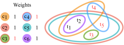
Figure 1. Hypergraph modelling of test coverage in Table 1. Faulty components and failing test cases are marked in red.

Suppose that we convert the execution traces in Table 1 to a hypergraph whose vertices and hyperedges correspond to test cases and program components, respectively. As shown in Figure 1, let each program component (hyperedge) connect all the test cases (vertices) which executed the program component. For example, $c_{1}=\{t_{1},t_{2},t_{4}\}$ and $c_{6}=\{t_{1},t_{2}\}$. The incidence matrix of the hypergraph in Figure 1 is then identical to the coverage matrix of the program under modelling:

(1) $$H=\left[\begin{array}[]{cccccc}1&1&0&0&1&1\\ 1&1&0&0&1&1\\ 0&1&1&0&1&0\\ 1&0&0&1&0&0\\ 0&1&0&1&1&0\\ \end{array}\right]$$

Thus, the hypergraph can model the test coverage without the loss of information.

Formally, given a set of program components $C$, a test suite $T$, and a coverage matrix $A$, we construct a hypergraph $G=(V,E,w)$ such that $V=T$, $E=\{\{t_{i}\in T|A_{ij}=1\}|c_{j}\in C\}$, $\forall e\in E.w(e)=1$. Then, the incidence matrix $H$ of $G$ satisfies $H=A$.

3.3. Defining Distance using a Hypergraph

There are several ways to measure the proximity between hypergraph vertices. In this work, referring to the recent article on hypergraph clustering (Whang et al., 2020), we first define the linkage between two vertices $v,v^{\prime}\in V$ by:

(2) $$l(v,v^{\prime})=\sum_{e\in E_{v}\cap E_{v^{\prime}}}\frac{w(e)}{deg(e)}$$

where $E_{v}=\{e\in E|v\in e\}$. As a hyperedge in $E_{v}\cap E_{v^{\prime}}$ connects fewer vertices and has the greater weight value, the linkage value will be higher; the linkage value encodes how tightly the two vertices are connected.

Since $E_{v}\cap E{v^{\prime}}\subseteq E_{v}$,

$$l(v,v^{\prime})=\sum_{e\in E_{v}\cap E_{v^{\prime}}}\frac{w(e)}{deg(e)}\leq\sum_{e\in E_{v}}\frac{w(e)}{deg(e)}=l(v,v)$$

Let us define $assoc(v):=l(v,v)$. Similarly, $l(v,v^{\prime})\leq assoc(v^{\prime})$. Therefore, we can normalise the linkage value in Eq. 2 as follows:

(3) $$\hat{l}(v,v^{\prime})=\frac{1}{2}\left(\frac{l(v,v^{\prime})}{assoc(v)}+\frac{l(v,v^{\prime})}{assoc(v^{\prime})}\right)$$

Then, $0\leq\hat{l}(v,v^{\prime})\leq 1$. We can simply prove that $\hat{l}(v,v^{\prime})=1$ when $E_{v}=E_{v^{\prime}}$, and $\hat{l}(v,v^{\prime})=0$ when $E_{v}\cap E_{v^{\prime}}=\emptyset$. This normalisation aims to measure the relative importance of the linkage between the two vertices, $v$ and $v^{\prime}$, compared to the total association of the vertices. There is another normalisation method dividing the linkage value by $deg(v)$ (Whang et al., 2020), not $assoc(v)$. However, we choose the denominator as $assoc(v)$ since it is a tighter upper bound on $l(v,v^{\prime})$ than $deg(v)$. Also, through our initial experiments, we have found that using $assoc(v)$ is more effective in failure clustering that using $deg(v)$ as a normalisation denominator.

The normalised linkage can be calculated in matrix form:

(4) $$\hat{L}=\frac{1}{2}\left((L\odot I)^{-1}L+L(L\odot I)^{-1}\right)$$

where $L=HWD_{e}^{-1}H^{T}$ is an unnormalised linkage matrix, and $\odot$ means the element-wise product. The matrix elements $L_{i,j}$ and $\hat{L}_{i,j}$ correspond to $l(v_{i},v_{j})$ and $\hat{l}(v_{i},v_{j})$, respectively.

Let us recall the motivating example in Section 2.1, which is modelled as a hypergraph in Figure 1. The normalised linkage values between the all pairs of vertices corresponding to failing tests, $T_{F}=\{t_{3},t_{4},t_{5}\}$, are as follows:

$$\hat{l}(t_{3},t_{4})=0,\hat{l}(t_{4},t_{5})=\textbf{0.55},\hat{l}(t_{3},t_{5})=0.42$$

In contrast to the vector- or set-based distance metrics in Section 2.2, the linkage values tell us that $t_{4}$ and $t_{5}$ has a stronger relationship than $t_{3}$ and $t_{5}$. This is because it incorporates the hyperedge degrees, which reflect the global coverage information. The more common a program component is, the more loosely the corresponding hyperedge is considered to connect the vertices.

Finally, we define the distance between the vertices based on the normalised linkage $\hat{l}$ (Eq. 2) by:

(5) $$\textit{hdist}(v,v^{\prime})=1-\hat{l}(v,v^{\prime})$$

As the linkage between vertices is stronger, the distance is smaller. For example, $t_{3}$ and $t_{4}$ (in Figure 1) do not share any hyperedges, so $\textit{hdist}(t_{3},t_{4})=1$, which is the maximum distance value. For all hypergraph vertices, the distance from itself is zero.

3.4. Subgraph Extraction using Failing Tests

Our original purpose is to cluster the set of failing test cases, i.e., to cluster a subset of vertices corresponding to failing test cases, $T_{F}$, and not the entire vertices $V=T$. Consequently, we eliminate the vertices of passing tests from the hypergraph while still preserving their information; this can reduce the computational cost of Eq. 4. To do so, we ensure that this elimination does not affect the distance between failing test cases by readjusting the weights of hyperedges.

Formally, given an original hypergraph $G=(V,E,w)$ modelling the test coverage, we reconstruct a hypergraph by including only vertices that correspond to failures and their adjacent hyperedges:

(6) $$G_{T_{F}}=(T_{F},\{e\cap T_{F}|e\in E\wedge e\cap T_{F}\neq\emptyset\},w^{\prime})$$

We call this subhypergraph as a restriction of $G$ to $T_{F}$.

In Section 3.3, hdist is defined in terms of $\hat{l}$, and $\hat{l}$ is defined in terms of $l$. Therefore, if we preserve $l$ between every pair of failing vertices, the distance does not change. Recall that the linkage $l(v,v^{\prime})$ is the sum of the ratio between the weight and the degree over all hyperedges connecting $v$ and $v^{\prime}$. Since the set of hyperedges among failing test vertices are the same in $G_{T_{F}}$, the only value needed to be preserved in $G_{T_{F}}$ is the ratio.

While the elimination of vertices may lead to the decrease in the degree of some hyperedge $e$, let $deg(e)$ be the degree of $e$ in $G$ and $deg^{\prime}(e)$ be the new degree of $e$ in $G_{T_{F}}$. Then, to preserve the ratio value, the new hyperedge weight $w^{\prime}(e)$ for all hyperedges $e$ in $G_{T_{F}}$ should satisfy the following equation:

(7) $$\frac{w^{\prime}(e)}{deg^{\prime}(e)}=\frac{w(e)}{deg(e)}$$

Since the original weights of all hyperedges are initially set to $1$ (in Section 3.2), Eq. 7 is equivalent to

(8) $$w^{\prime}(e)=\frac{deg^{\prime}(e)}{deg(e)}(\because\forall e.w(e)=1)$$

Mathematically, $w^{\prime}(e_{j})$ is equivalent to $\frac{|\{t_{i}\in T_{F}|A_{ij}=1\}|}{|\{t_{i}\in T|A_{ij}=1\}|}$, which is the ratio of failing test cases among all test cases covering the corresponding program component $c_{j}$.

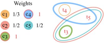
Figure 2. Restriction of the hypergraph in Figure 1 to vertices corresponding to failing tests. The thickness of each hyperedge is proportional to its readjusted weight.

Figure 2 shows the restriction of the hypergraph in Figure 1 with the readjusted weights of the hyperedges, $(\frac{1}{3},\frac{1}{2},1,1,\frac{1}{2})$. The incidence matrix of this reduced hypergraph is a submatrix of $H$ (in Eq. 1) formed by the rows and the columns that correspond to the remaining vertices and hyperedges, respectively:

$$H_{3:5,1:5}=\left[\begin{array}[]{ccccc}0&1&1&0&1\\ 1&0&0&1&0\\ 0&1&0&1&1\\ \end{array}\right]$$

Finally, the pairwise distance matrices, i.e. $1-\hat{L}$, before and after the restriction are as follows:

$$\left[\begin{array}[]{ccccc}0.00&0.00&0.53&0.60&0.45\\ 0.00&0.00&0.53&0.60&0.45\\ 0.53&0.53&\textbf{0.00}&\textbf{1.00}&\textbf{0.58}\\ 0.60&0.60&\textbf{1.00}&\textbf{0.00}&\textbf{0.45}\\ 0.45&0.45&\textbf{0.58}&\textbf{0.45}&\textbf{0.00}\\ \end{array}\right]\rightarrow\left[\begin{array}[]{ccc}\textbf{0.00}&\textbf{1.00}&\textbf{0.58}\\ \textbf{1.00}&\textbf{0.00}&\textbf{0.45}\\ \textbf{0.58}&\textbf{0.45}&\textbf{0.00}\\ \end{array}\right]$$

The restriction does not alter the distance between failing test cases.

3.5. Agglomerative Hierarchical Clustering

We use a hierarchical clustering algorithm instead of partitional clustering algorithms such as K-means (Kanungo et al., 2002). When the number of faults is not known in advance, the freedom to derive any number of clusters from a single application of hierarchical clustering algorithm can be beneficial (Golagha et al., 2019). Users can examine the resulting dendrogram using their domain knowledge and find an appropriate stopping point. Many existing failure clustering techniques also use hierarchical clustering due to the same reasons (Jones et al., 2007; Golagha et al., 2017; Golagha et al., 2019).

We follow the typical Agglomerative Hierarchical Clustering (AHC) process: it starts with each failing test case being set as an individual cluster and merges the two closest clusters at each iteration. When the distance between two tests $t$ and $t^{\prime}$ is given as $dist(t,t^{\prime})$, there are several ways to define the intercluster distance between two clusters $C$ and $C^{\prime}$. In this work, we compare the three linkage methods defined in Table 2 that aggregate the distance between all vertex pairs in $C$ and $C^{\prime}$. Note that any pairwise test distance function including hdist can be plugged into $dist$.

Table 2. Different options of the intercluster distance

Name	Definition
Average (avg)	$D_{dist}(C,C^{\prime})=\frac{1}{|C||C^{\prime}|}\sum_{t\in C,t^{\prime}\in C^{\prime}}dist(t,t^{\prime})$
Single (min)	$D_{dist}(C,C^{\prime})=\min_{t\in C,t^{\prime}\in C^{\prime}}dist(t,t^{\prime})$
Complete (max)	$D_{dist}(C,C^{\prime})=\max_{t\in C,t^{\prime}\in C^{\prime}}dist(t,t^{\prime})$

Algorithm 1 formally depicts the agglomerative clustering process. In our approach, we set the input parameter $D_{dist}$ to $D_{hdist}$. As mentioned earlier, the algorithm begins with $|T_{F}|$ clusters in which each failing test case is set to an individual cluster (Line 2). Then, in each iteration, the nearest clusters are combined (Line 4-6). This process continues until the number of clusters becomes $1$ (Line 3). Finally, it returns the clustering results of test cases and the minimum distance results from every iteration (Line 9). Note that $P_{k}$ denotes the size $k$ partition of $T_{F}$, and $mdist_{k}$ is the minimum intercluster distance when there are $k$ clusters.

Input: Failing test cases $|T_{F}|$, Intercluster distance function $D_{dist}$

Output: Clustering results $P_{1}$, …, $P_{N}$, Mininum distance results $mdist_{2}$, …, $mdist_{N}$

1 $N\leftarrow|T_{F}|,k\leftarrow|T_{F}|$

2 $P_{k}\leftarrow\{\{t\}|t\in T_{F}\}$

3 while $k>1$ do

4       $C_{1},C_{2}\leftarrow argmin_{C\in P_{k},C^{\prime}\in P_{k},C\neq C^{\prime}}D_{dist}(C,C^{\prime})$

5       $mdist_{k}\leftarrow D_{dist}(C_{1},C_{2})$

6       $P_{k-1}\leftarrow(P_{k}\setminus\{C_{1},C_{2}\})\cup\{C_{1}\cup C_{2}\}$

7       $k\leftarrow k-1$

8 end while

return $\{P_{1},\dots,P_{N}\}$, $\{mdist_{2},\dots,mdist_{N}\}$

Algorithm 1 Agglomerative clustering of failing test cases

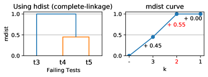
Figure 3. Dendrogram (left) and $mdist$ curve (right) for the failure clustering results of Figure 2 (hdist-complete used), Since $mdist_{k}$ can be defined only when $k>1$, $mdist_{1}$ is simply set to $1$, which is the upper bound of hdist.

For example, if we run this algorithm on the previous example (Figure 2) with the Complete intercluster distance, $P_{3}$ and $P_{2}$ will be $\{\{t_{3}\},\{t_{4}\},\{t_{5}\}\}$ and $\{\{t_{3}\},\{t_{4},t_{5}\}\}$, respectively, while $mdist_{3}=0.45$ and $mdist_{2}=1.0$. The clustering results can be represented as a dendrogram as shown in Figure 3. The curve of $mdist$ according to the number of clusters $K$ can be deduced from the dendrogram. If we cut this dendrogram at the distance threshold $0.8$, the number of clusters is two, and the failing test cases can be perfectly clustered.

Although users can manually decide the number of clusters from the dendrogram, the clustering tool would be more useful if it can assist users by automatically suggesting the proper number of clusters. The simplest way might be setting the distance threshold to a fixed value that works best empirically. On the other hand, in previous work (Jones et al., 2007; Golagha et al., 2017), the stopping criterion is defined based on the fault localisation results.

In this work, we choose a stopping point using the elbow method which is widely used to determine the number of clusters. The elbow point of a curve is loosely defined as ”the point of maximum curvature” (Salvador and Chan, 2004), so there is no universally accepted definition, but instead there are various heuristic approaches (Satopaa et al., 2011; Salvador and Chan, 2004; Zambelli, 2016; Antunes et al., 2018) to find the point. We use one variant of them, which defines an elbow point as the point near the maximum amount of difference (equal to Maximum Difference in Zambelli et al. (Zambelli, 2016)). Formally, we apply the elbow method on the mdist curve: it stops at the number of clusters $k$ right before the largest increase of minimum intercluster distance, defined as follows:

(9) $$k=argmax_{1\leq k\leq N}\left(mdist_{k}-mdist_{k+1}\right)$$

where $mdist_{1}$ and $mdist_{N+1}$ are set to $0$ and $1$, respectively, assuming that we use a normalised distance metric. For example, if this is applied to the $mdist$ curve in Figure 3, the suggested number of clusters is two because the maximum difference is 0.55 ($=mdist_{2}-mdist_{3}$). This method assumes that once the test cases are optimally clustered, the increase in the minimum intercluster distance would be substantially high.

4. Experimental Setup

Using our Java and C multi-fault datasets, we compare the performance of our hypergraph-based method to other approaches, including MSeer, in terms of the effectiveness and efficiency for failure clustering and also the improvement in SBFL performance.

4.1. Construction of multi-fault Dataset

We construct multi-fault datasets using the existing fault datasets Defects4J (Just et al., 2014) and Software-artifact Infrastructure Repository (SIR) (Do et al., 2005; LLC, [n.d.]). Table 3 shows the number of faulty subjects used in our experiment. As well as the multi-fault data (# faults ¿ 1), we also include the single fault data (# faults = 1) that have multiple failing test cases. This is because we also need to check whether a clustering algorithm assigns multiple failing test cases that share a single root cause to the same cluster, instead of dividing them into separate clusters. Section 4.1.1 and Section 4.1.2 explain the multi-fault data creation process for Java and C programs, respectively. We measure the statement-level test coverage for all subjects using Cobertura for Java and gcov for C. Note that we make the failure-to-single-fault assumption, as in previous work on failure clustering (Podgurski and Yang, 1993; Liu and Han, 2006; Bowring et al., 2004): we expect each of the failing test cases to have a single root cause.

Table 3. Experiment Dataset ($M$ = # lines)

Base Dataset	# Faults							$M$	$|T_{F}|$
	1	2	3	4	5	6	7
Defects4J (Java)	124	240	79	16	9	5	2	24069.6	4.8
SIR (C)	54	54	19	3	-	-	-	1934.3	31.6
Total	178	294	98	19	9	5	2	-	-

4.1.1. Java faults

Defects4J (Just et al., 2014) is a real-world faults dataset from various open-sourced Java programs. We use the five projects, Lang, Chart, Time, Math and Closure, to construct our multi-fault dataset.

Each buggy version of the program in Defects4J has a set of failing test cases that reveals a single fault in the program. After applying the provided revision patch on the buggy version, all fault-revealing test cases do not fail anymore. All buggy versions of a project are sorted chronologically by the date of revision, and the more recently a bug is fixed, the lower the bug ID is assigned. Therefore, in a project, it is likely that a buggy program with a higher bug ID already contains the faults in the buggy programs with lower bug IDs, which is not yet detected due to the absence of fault-revealing test cases for the faults. For example, the more recently fixed faults, Math-3 and Math-4, already exist in the older version Math-5. We include such buggy versions that already contain multiple faults to our dataset.

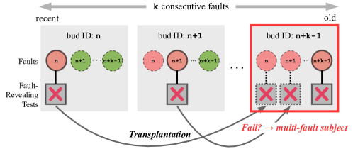
Figure 4. Building Java multi-fault dataset using Defects4J

Since it is cumbersome to manually validate whether each fault exists in the older version, we use the results of the fault-revealing test cases of the fault. As shown in Figure 4, suppose that there are $k$ consecutive buggy programs ($k>1$) whose fault-revealing test cases are non-overlapping due to the failure-to-single-fault assumption. For $i=0,\dots,k-2$, we transplant the code snippets of fault-revealing test cases from the more recent buggy versions, $\{n,\dots,n+k-2\}$, to the oldest buggy version $n+k-1$. After the transplantation, we regard that a fault $n+i$ exists in the buggy version $n+k-1$ if all fault-revealing test cases of the fault are still compilable and fail on the version.

If all faults are considered to exist, we add the constructed multi-fault subject (the buggy version $n+k-1$ with the $k$ sets of failing test cases) to our dataset. Once we succeed to generate the $k$-faults subject from the buggy versions $\{n,\dots,n+k-1\}$, we successively try to combine $k+1$ faults using the versions $\{n-1,\dots,n+k-1\}$.

4.1.2. C faults

In addition to the Java fault dataset, we use four C subject programs from SIR (Do et al., 2005; LLC, [n.d.]) that is a widely-used debugging benchmark and also employed in the previous failing clustering work (DiGiuseppe and Jones, 2012; Gao and Wong, 2017): version 1.5 of gzip, version 1.2 of grep, version 1.1 of flex, and version 2.0 of sed. The benchmark contains artificial faults seeded on a correct version of a program. Each faulty region can be either activated or deactivated using macro definitions and preprocessors, i.e., ifdef, or ifndef. Note that a fault can span multiple (not necessarily continuous) lines, sharing the same root cause. Because those faulty regions are distinct from each other, multi-fault programs can be constructed by simultaneously activating the multiple faulty lines. Then, we observe the failing tests of the combined faults.

After combining the faults, in some cases, fault interference (Debroy and Wong, 2009; DiGiuseppe and Jones, 2011) makes it difficult to clearly define the membership of some failing test cases. For example, if a test case that is failing in the combined version was initially passed with any of the single faults, it is hard to assign the cluster membership of the test case to only one fault since the presence of multiple faults makes the test fail. Under the failure-to-single-fault assumption, we exclude such failing test cases from our evaluation dataset. Similarly, only non-overlapping failing test cases of the faults are set to the target of clustering. We include only the multi-fault subjects of which each fault is not entirely masked (Debroy and Wong, 2009; Jones et al., 2007) by other faults; therefore, all faults of the subjects can be discoverable by at least one failing test case.

Additionally, failing test cases which crashed due to illegal memory access (segmentation fault) are omitted since coverage data is not generated on those executions using gcov.

4.2. Evaluation Methodology

4.2.1. Clustering Performance

When the ground-truth clustering is unknown, the quality of clustering is typically evaluated by internal criteria such as the degree of cluster cohesion or separation. However, satisfying the internal criteria does not always guarantee high effectiveness in an application (Cambridge, 2009). In our multi-fault datasets, since we know which failing tests are fault-revealing tests of which fault, we could regard that information as ground-truth. Thereby, instead of internal criteria, we use external criteria which directly compare the clustering results with the ground-truth clusters.

In Section 2, we introduced two external criteria: Homogeneity ($h$) and Completeness ($m$) (Rosenberg and Hirschberg, 2007). Given ground-truth clusters $P_{GT}=\{T_{1},\dots,T_{c}\}$ and arbitrary clusters $P=\{T^{\prime}_{1},\cdots,T^{\prime}_{k}\}$ that are both partitions of $T_{F}$, the two criteria are formally defined by:

(10) $$h(P,P_{GT})=1-\frac{H(P_{GT}|P)}{H(P_{GT})}$$

(11) $$m(P,P_{GT})=1-\frac{H(P|P_{GT})}{H(P)}$$

In Eq. 10, $H(P_{GT}|P)$ means the conditional entropy of the clusters $P_{GT}$ given the clusters $P$, and $H(P_{GT})$ is an entropy of $P_{GT}$:

$$\small H(P_{GT}|P) =-\sum_{i=1}^{c}\sum_{j=1}^{k}\frac{|T_{i}\cap T^{\prime}_{j}|}{|T_{F}|}log\frac{|T_{i}\cap T^{\prime}_{j}|}{|T^{\prime}_{j}|}$$

$$H(P_{GT}) =-\sum_{i=1}^{c}\frac{|T_{i}|}{|T_{F}|}log\frac{|T_{i}|}{|T_{F}|}$$

Similarly, $H(P|P_{GT})$ and $H(P)$ in Eq. 11 are defined in a symmetric way. Both $h$ and $m$ values are bounded in the range from 0 (worst) to 1 (best). A clustering is perfect if and only if both $h$ and $m$ are 1.

A most widely-used external criterion in literature is normalised mutual information (NMI) (Vinh et al., 2010), which measures the agreement between two clustering assignments. Interestingly, it has been found that NMI is mathematically equivalent to the harmonic mean of Homogeneity and Completeness, i.e., $\frac{2(h+m)}{h\cdot m}$ (the proof is in (Becker, 2011)). Therefore, we use NMI to evaluate failure clustering effectiveness.

4.2.2. Fault Localisation Performance

Once we cluster the multiple failing test cases, following the parallel debugging process (Jones et al., 2007), we generate a suspiciousness ranking from each cluster using the failing test cases in the cluster along with all passing test cases. The $k$ rankings obtained from $k$ failure clusters can be investigated by multiple developers in a parallel manner, assigning the ranking from each cluster to a developer who is most responsible for the cluster’s failing test cases. Once developers finish inspecting all rankings and fix the found faults, the next iteration can begin with remaining failing test cases. In this work, we evaluate the fault localisation performance of the first iteration of parallel debugging.

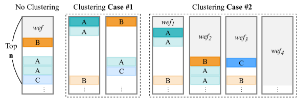
Figure 5. The example of the parallel debugging process

Given a ranking, let us assume that developers inspect only the program components within the top $n$ (complying with the guideline from Parnin and Orso  (Parnin and Orso, 2011)) until finding the highest-ranked faulty component. A fault is considered to be found when it is associated with at least one of the highest-ranked faulty components of the rankings. For example, in Figure 5, two faults, $\{A,B\}$, and three faults, $\{A,B,C\}$, are found in Case #1 and #2, respectively. Note that a fault may span multiple components, e.g., consecutive lines.

Wasted effort ($\textit{wef}_{i}$) for the $i$-th ranking is defined as the number of program components should be examined before finding the highest-ranked faulty component in the ranking (Figure 5). If no faulty component exists within top $n$, $\textit{wef}_{i}$ is $n$. Then, the total wasted effort (t-wef) is defined as the sum of $\textit{wef}_{i}$ for all rankings: $\textit{t-wef}=\sum_{i=1}^{k}\textit{wef}_{i}$. For example, t-wef of Case #1 is less than the one of Case #2 in Figure 5. A lower t-wef means better efficiency of fault localisation. We also compute the percentage of rankings that cannot rank at least one faulty element higher than other rankings. We call such rankings as redundant rankings.

We use two FL techniques, Ochiai (Abreu et al., 2009) and Crosstab (Wong et al., 2008). Since our Java subjects have much more lines than C subjects, we use the method-level rankings while the suspiciousness score of each method is set to the maximum suspiciousness of its lines.

4.3. Other Clustering Methods for Comparison

Hybiscus is compared with following failure clustering methods:

• MSeer (Gao and Wong, 2017): A recently proposed failure clustering technique using the K-medoids algorithm with own technique for estimating $K$. Revised Kendall-Tau (RKT) distance is used to calculate the distance between failing test cases.

• Test Class Name (TCN): Assigning the cluster membership of failing test case methods according to the classes of them (only for Java subjects)

• Agglomerative Hierarchical Clustering (AHC) with other distance metrics: Jaccard, Sørensen-Dice, Cosine, Euclidean, Hamming, and RKT (used in MSeer).

5. Result and Analysis

To evaluate Hybiscus, we set up the following research questions:

• RQ1. Distance Metric: How effective is hdist when compared to other distance metrics in failure clustering?

• RQ2. Stopping Criteria: How accurate is the failure clustering with our stopping criterion when compared to other clustering approaches?

• RQ3. Efficiency: How efficient is the calculation of hdist when compared to other distance metrics?

• RQ4. FL accuracy: How does the accuracy of failure clustering affect SBFL performance?

In the following sections, we present answers to our research questions. Full results are available at our repository.

5.1. RQ1: Distance Metric

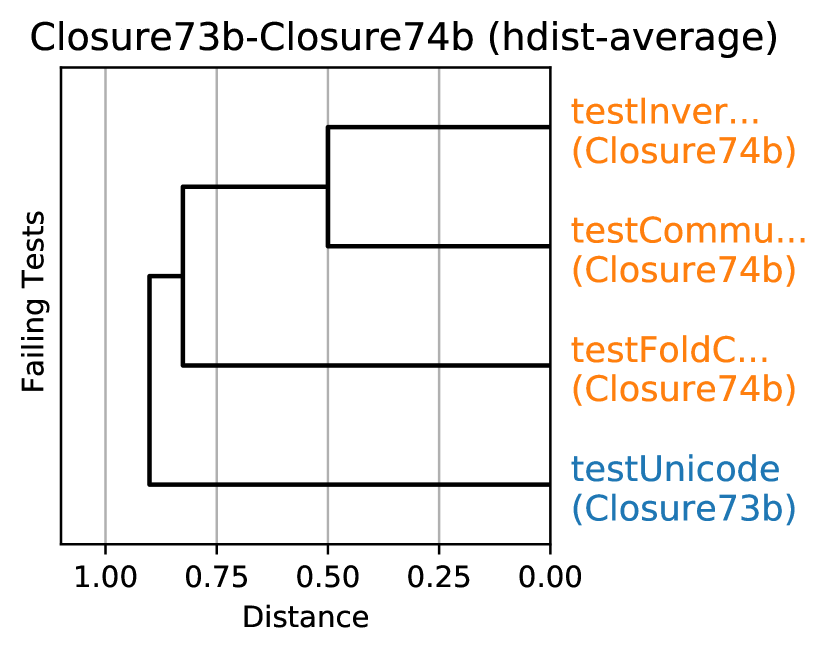
(a) Using hdist-average

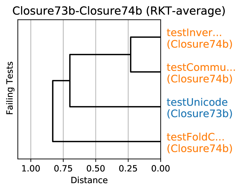
(b) Using RKT-average

Figure 6. Dendrogram for Closure73b-Closure74b

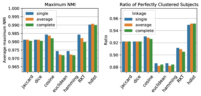
(a) On 475 Java subjects

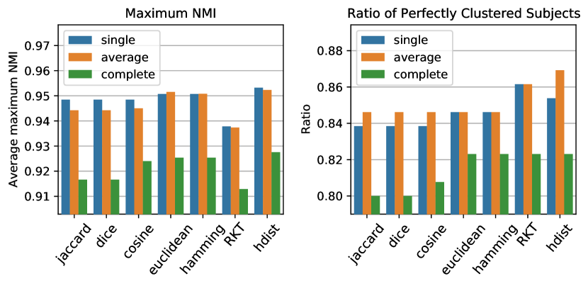
(b) On 130 C subjects

Figure 7. Averaged maximum NMI (left) and the ratio of perfectly clustered subjects (right). Note that the ranges of the y-axis are different.

To answer RQ1, we compute the maximum NMI values among all iterations of AHC without considering stopping criteria. In addition, we check whether the failing test cases of each faulty subject are perfectly clustered at any stopping point of AHC. For example, in Figure 6, the maximum NMI of hdist is $1$, as failing tests are perfectly clustered after two merges (# clusters = 2). In comparison, the maximum NMI of RKT is $0.70$ (# clusters = 3), and the failing tests are not perfectly clustered with any number of clusters.

Figure 7 shows the maximum NMI values averaged over all subjects (left) and the ratio of perfectly clustered subjects (right). This can be regarded as a performance measure of failure clustering with an optimal stopping criterion for each distance metric. Note that 34.5% of Java subjects and 9.2% of C subjects have only two failing test cases, always resulting in perfect clustering (e.g., NMI = 1). Excluding those subjects, on Java, hdist-average outperforms other distance metrics in terms of NMI; NMI values of hdist-average are significantly higher than ones of RKT-single (dependent $t$-test for paired samples with p=0.023). On C, hdist-single and -average show higher mean values when compared to other distance metrics, but the differences are not statistically significant. In terms of the perfectly clustered ratio, hdist-average shows the best performance: it perfectly clusters about 95% and 87% of Java and C subjects, respectively, in one of the stopping points in AHC.

Interestingly, we observe that RKT does not always outperform set- or vector-based distance metrics, which is inconsistent with the core idea of Gao and Wong (Gao and Wong, 2017) that assumes that ranking-based distance metrics will outperform other distance metrics.

Answer to RQ1: hdist (especially with average linkage) outperforms other distance metrics for failure clustering.

5.2. RQ2: Stopping Criteria

Table 4. Failure clustering performance using Eq. 9 for AHC (k = # clusters, c = # actual faults, h = homogeneity, m = completeness, Perf. = the ratio of perfectly clustered subjects)

Clustering Method		Java					C
		$k/c$	h	m	NMI	Perf.	$k/c$	h	m	NMI	Perf.
MSeer		1.67	0.985	0.601	0.644	0.406	3.19	0.855	0.479	0.427	0.246
TCN		1.26	0.950	0.818	0.802	0.646	-	-	-	-	-
Jacc.	min	1.02	0.826	0.907	0.753	0.674	0.86	0.688	0.967	0.670	0.585
	avg	1.03	0.830	0.901	0.753	0.669	0.88	0.694	0.959	0.669	0.585
	max	1.04	0.840	0.894	0.761	0.674	0.90	0.728	0.952	0.693	0.615
Dice	min	0.90	0.717	0.953	0.685	0.621	0.79	0.616	0.993	0.620	0.554
	avg	0.92	0.721	0.946	0.684	0.619	0.82	0.645	0.974	0.638	0.562
	max	0.94	0.729	0.935	0.686	0.615	0.83	0.654	0.967	0.633	0.577
Cos.	min	0.88	0.701	0.962	0.676	0.617	0.77	0.569	0.987	0.566	0.508
	avg	0.90	0.702	0.957	0.673	0.615	0.78	0.578	0.978	0.567	0.523
	max	0.91	0.709	0.950	0.675	0.613	0.81	0.622	0.968	0.602	0.562
Ham.	min	0.88	0.690	0.926	0.641	0.560	0.76	0.578	0.992	0.582	0.508
	avg	0.89	0.704	0.916	0.658	0.564	0.80	0.615	0.980	0.613	0.531
	max	0.93	0.746	0.899	0.698	0.577	0.82	0.650	0.955	0.637	0.531
RKT	min	1.36	0.957	0.705	0.697	0.539	1.26	0.831	0.802	0.646	0.577
	avg	1.42	0.971	0.689	0.695	0.531	1.82	0.900	0.710	0.627	0.538
	max	1.42	0.976	0.673	0.686	0.524	2.39	0.938	0.561	0.530	0.408
hdist	min	1.20	0.949	0.848	0.826	0.678	0.86	0.718	0.989	0.713	0.677
	avg	1.21	0.958	0.846	0.833	0.680	0.94	0.798	0.971	0.776	0.731
	max	1.22	0.963	0.839	0.832	0.680	1.35	0.846	0.835	0.709	0.585

For AHC, we determine the number of clusters, $k$, using our stopping criterion defined in Eq. 9. Table 4 shows the failure clustering performance of AHC and the other clustering methods, MSeer and TCN, described in Section 4.3. The second column shows the method of defining the intercluster distance. Euclidean distance is excluded since it is not normalised.

With our stopping criterion, AHC with hdist-average outperforms other clustering approaches on both Java and C datasets in terms of NMI and the ratio of perfectly clustered subjects (Perf.). It perfectly maps failures to their root causes for 68% and 73% of the studied Java and C subjects, respectively. Since RQ1 shows that the upper-bounds of Perf. are 95% and 87%, there is still room for improvement of a stopping criterion. We have evaluated the other two stopping criteria: stopping after reaching some distance threshold (threshold-based) and at maximum modularity of pairwise distance graph (Blondel et al., 2008) (modularity-based). Briefly, the modularity-based criterion shows poorer performance than our stopping criterion for every distance metric. Meanwhile, the threshold-based criterion shows a discrepancy between best-performing thresholds on Java and C subjects, even though their NMI scores are higher than our stopping criterion: hdist-single with the threshold 0.65 shows the best NMI score, 0.86, on Java, while hdist-single with the threshold 0.45 shows the best NMI score, 0.79, on C. We need further research to understand the features of faulty programs that could be used to determine a good distance threshold.

On both Java and C subjects, MSeer tends to generate many more clusters than the actual number of faults. The clusters of MSeer show relatively high homogeneity, but lower completeness than all others, which means the failing tests due to the same fault is likely to split into different clusters. Interestingly, AHC-RKT with our stopping criterion outperforms MSeer that also uses RKT. We note that TCN performs relatively well for Java. Since related tests are likely to be put in the same class, TCN can be viewed as ”manual clustering” by developers. However, we expect its performance to depend heavily on the organisation of the test classes.

Answer to RQ2: Using our stopping criterion, especially with hdist-average, outperforms the TCN baseline and the existing failure clustering approach, MSeer.

5.3. RQ3: Efficiency

Figure 8 shows the log-scaled distribution of distance calculation time on all studied subjects. Note that the cost of hdist includes not only the distance computation but also the hypergraph modelling and the subgraph extraction process. For every subject, calculating hdist requires one second at most. In Figure 9, we present the cost analysis of hdist using linear regression. The required computation time is approximately linear to $M$, $M^{\prime}$ and $|T_{F}|^{2}$: $\textit{time}(s)=10^{-5}\times(3.09M^{\prime}+0.84M^{\prime}+0.15|T_{F}|^{2})$ ($R^{2}=0.9123$), where $M$ is total number of program components, and $M^{\prime}$ is the number of program components executed by at least one failing test case, i.e., the number of hyperedges in $G_{T_{F}}$ (Eq. 6).

The computation of RKT, on the other hand, remains expensive despite efforts for optimisation: it can takes more than 10,000 seconds (i.e., more than 2.7 hours) to calculate distances between failing tests for some of the large subjects. For example, it takes 5.6 hours (2.5 hours with GPU parallelisation) to calculate RKT distances between failing tests of Closure49b-50b that has 38,235 executed lines and 68 failing test cases. In comparison, hdist only takes 0.49 seconds. Unlike hdist that is roughly linear to $M$, RKT shows $O(M^{2}|T_{F}|^{2})$ time complexity.

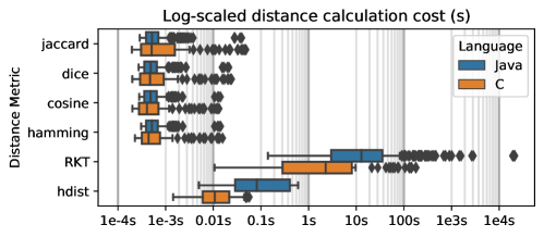
Figure 8. Distribution of distance calculation cost (log-scale)

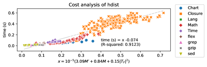
Figure 9. Analysis of hdist calculation time (s)

Answer to RQ3: Even though the cost of hdist calculation is higher than the set- or vector-based metrics, it is still negligible even in the large subjects, while RKT requires much more computation time.

Table 5. FL performance after the failure clustering (using Ochiai, max tie-breaker). R.R. means Redundant Rankings.

Method			R.R.	The ratio of found faults (t-wef)
Java (method-level)				n=1	n=5	n=10	n=$\infty$
No Clustering			-	0.13 (0.73)	0.34 (2.56)	0.38 (3.88)	0.50 (21.6)
MSeer			19.2%	0.37 (2.11)	0.75 (7.07)	0.82 (11.19)	0.98 (285.9)
TCN			9.2%	0.33 (1.71)	0.73 (5.48)	0.80 (8.62)	0.97 (234.1)
	Jacc.	min	4.2%	0.31 (1.34)	0.68 (4.16)	0.74 (6.36)	0.91 (162.3)
		avg	4.4%	0.31 (1.36)	0.68 (4.22)	0.74 (6.48)	0.91 (177.2)
		max	4.6%	0.31 (1.38)	0.68 (4.28)	0.74 (6.55)	0.92 (191.9)
A	RKT	min	12.8%	0.35 (1.72)	0.74 (5.50)	0.80 (8.53)	0.97 (241.5)
H		avg	13.2%	0.35 (1.77)	0.75 (5.61)	0.81 (8.67)	0.97 (249.9)
C		max	14.0%	0.35 (1.78)	0.75 (5.70)	0.81 (8.81)	0.98 (250.6)
	hdist	min	6.0%	0.35 (1.56)	0.73 (4.86)	0.79 (7.45)	0.97 (181.2)
		avg	6.7%	0.35 (1.59)	0.73 (4.99)	0.80 (7.70)	0.97 (234.1)
		max	6.3%	0.36 (1.60)	0.74 (5.02)	0.80 (7.80)	0.98 (235.6)
C (line-level)				n=5	n=10	n=15	n=$\infty$
No Clustering			-	0.05 (4.8)	0.09 (9.0)	0.12 (13.1)	0.73 (342.5)
MSeer			41.1%	0.06 (22.2)	0.14 (43.0)	0.17 (63.2)	0.91 (2698.1)
	Jacc.	min	3.5%	0.05 (7.1)	0.11 (13.6)	0.15 (19.7)	0.87 (444.5)
		avg	4.3%	0.05 (7.2)	0.11 (13.8)	0.15 (20.0)	0.87 (467.6)
		max	4.8%	0.06 (7.7)	0.12 (14.7)	0.16 (21.1)	0.89 (462.1)
A	RKT	min	14.7%	0.05 (10.5)	0.13 (20.2)	0.17 (29.6)	0.94 (706.8)
H		avg	22.6%	0.04 (15.0)	0.13 (29.3)	0.16 (43.1)	0.96 (1747.0)
C		max	32.6%	0.04 (18.3)	0.13 (35.9)	0.16 (52.8)	0.98 (2137.1)
	hdist	min	2.3%	0.06 (7.3)	0.13 (13.9)	0.17 (20.1)	0.89 (480.8)
		avg	4.4%	0.05 (8.2)	0.13 (15.6)	0.17 (22.5)	0.93 (508.1)
		max	15.0%	0.05 (11.7)	0.13 (22.3)	0.17 (32.1)	0.96 (653.6)

5.4. RQ4: FL Accuracy

Table 5 shows the FL performance using Ochiai after the failure clustering. The lowest ranks are assigned to the program components with equal suspiciousness scores (max tie-breaker). We do not present the results of Dice, Cosine, and Hamming because using each of them found fewer faults than using Jaccard. Note that Eq. 9 is used as a stopping criterion for AHC.

The results show that we can find more faults with failure clustering. Especially, MSeer, AHC-RKT, and AHC-hdist similarly find the greatest number of faults: when $n=10$, about 80-82% and 13-14% of faults can be found on Java and C subjects, respectively. In RQ2, we show that MSeer and AHC-RKT produce more homogeneous but less complete clusters than AHC-hdist. Although there is less noise when performing FL due to the higher homogeneity, fewer failing test cases of a fault are utilised in FL due to the lower completeness. This paucity of information may degrade FL accuracy so that a similar number of faults being found by MSeer and AHC-RKT when compared to AHC-hdist despite their higher homogeneity. Meanwhile, the lower completeness also make MSeer and AHC-RKT produce more redundant rankings than AHC-hdist. This, in turn, leads to a higher inspection cost, t-wef. In fact, AHC-hdist (with the single linkage method) requires only 63% and 18% of t-wef than MSeer (when $n=\infty$) on Java and C subjects, respectively. Consequently, AHC-hdist shows higher efficiency than the other methods that found a similar number of faults.

Answer to RQ4: The more homogeneous a cluster is, the more effective the FL is. Similarly, the more complete a cluster is, the more efficient the FL is (as pointed out in Section 2).

6. Threats to Validity

Threats to internal validity concern factors that may influence the observed effects, such as the integrity of the coverage and test result data, as well as failure clustering and fault localisation. To minimise threats, we use Cobertura and gcov, both widely used coverage profilers. We also make both our implementation and datasets publicly available for further scrutiny.

Threats to external validity concern any factor that may limit the generalisation of our results. Our results are based on Defects4J and SIR: both have been widely studied in conjunction with automated debugging techniques, and facilitate a direct comparison between our results and other existing work. However, only further studies with more diverse programs and faults can strengthen claims for generalisation. Additionally, the reported results are strictly based on the failure-to-single-fault assumption (DiGiuseppe and Jones, 2012), and may not generalise for multiple-fault failures (Yu et al., 2015). We will consider overlapping clustering (Xie et al., 2013; Whang et al., 2018; Yang and Leskovec, 2013; Whang et al., 2016) to handle such cases in the future. Our findings about hdist are based on hierarchical clustering, and may not generalise to partitional clustering algorithms. Finally, our results are based on coverage measured at the statement level: the findings may not generalise to coverage measured at other granularity levels. We expect coarser-grained coverage criteria such as method or file coverage to perform worse, as they contain less information about the test behaviour. Since the statement coverage is one of the most widely used type of coverage in practice, we believe the current experimental design can provide the most accurate evaluation of the proposed distance metric that is also practically relevant. A more thorough evaluation of the use of coarser-grained coverage metrics in situations where statement level coverage is not available will allow us to evaluate how much the clustering accuracy degrades due to the change of granularity. We leave this as future work.

Finally, threats to construct validity concern the use of metrics that may not reflect the properties we intend to measure. All evaluation metrics for clustering (homogeneity, completeness, and NMI) are widely used in the literature, leaving little room for misunderstanding. Following Parnin and Orso (Parnin and Orso, 2011), we report count based metrics for FL, under the assumption that developers will inspect only the first few elements in the suspiciousness ranking.

7. Related Work

We present related work in failure clustering for debugging and hypergraph clustering algorithms.

7.1. Coverage-based Failure Clustering

Podgurski et al.  (Podgurski et al., 2003) showed that the coverage profile could be used to group failures that share root causes. Jones et al. (Jones et al., 2007) defined a parallel-debugging process, which produces fault-focused clusters of failing test cases to parallelise the task of debugging faults. They proposed two techniques for clustering, either representing a failing test as a behaviour model or a suspiciousness ranking. The second technique, often used for baseline comparison in several later work (Steimann and Frenkel, 2012; Gao and Wong, 2017), employs Tarantula (Jones et al., 2002) with each failing test and all passing tests to generate rankings, and measure the similarity between them using Jaccard. Golagha et al. (Golagha et al., 2017) adapt the parallel-debugging process into a real context with a high cost of test execution, and suggest using only a representative test from each cluster rather than utilising all failing tests for debugging. They do not evaluate automated FL performance after failure clustering.

Recently, Gao and Wong proposed MSeer (Gao and Wong, 2017), which defines the profile of a failing test case as a suspiciousness ranking in a similar manner with Jones et al. (Jones et al., 2007). They use a revised Kendall-Tau distance that performs better than Jaccard distance in comparing rankings and employ the K-medoids clustering algorithm, using their own method of estimating the number of clusters.

Some work (Steimann and Frenkel, 2012; Högerle et al., 2014) suggests a partitioning method that divides both failing tests and program elements using algorithms borrowed from integer linear programming. They only account for failing test cases, thus not considering the differing importance of program components as mentioned in Section 2.2.

7.2. Non Coverage-based Failure Clustering

There are several existing work in clustering crashes or failing tests (Dang et al., 2012; Pham et al., 2017; van Tonder et al., 2018; Golagha et al., 2019) without coverage information. Dang et al. (Dang et al., 2012) proposed ReBucket that clusters duplicate crash reports using call stacks. They designed a novel metric called Position Dependent Model to measure the similarity between two crash call stacks. However, this method can be applied to only crash failures, and not to other failures such as assertion violations associated with test oracles. Pham et al. (Pham et al., 2017) proposed a symbolic execution-based failure clustering method. Instead of clustering crash or bug reports, it clusters the failing test cases generated during the symbolic execution while assuming no provided bug-revealing test input. Since their approach is plugged into the main loop of a symbolic execution engine, it cannot be easily applied to general test cases written by developers. Tonder et al. (van Tonder et al., 2018) presented an approach to bucket crashing inputs produced by fuzzers. It transforms a program under test to characterise crashes based on the idea that a correct fix can group crashing inputs triggered by the same, unique bug. They evaluated their approach on six real-world projects with three different fuzzers. Although utilising semantic analysis of a failure for failure clustering can yield precise results, this approach also requires frequent recompiling and execution of the program under test to validate fixes, which may limist its scalability to industry-level projects. In contrast, our distance metric, hdist, and failure clustering technique, Hybiscus, only require the coverage information and do not incur any other expensive analysis cost. Golagha et al. (Golagha et al., 2019) used non-code features to cluster failing test cases. They cluster the test failure utilising general test features such as identifiers, component membership, history data of test execution, broken/repaired features, or data collected from the associated issue tracker such as Jira. While this method does not require the cost of coverage measurement, it cannot be applied to projects without sufficient issue tracking history, limiting its applicability to mature projects.

7.3. Hypergraph Clustering

Hypergraph clustering is considered an important problem in the fields of data mining and machine learning (Saito et al., 2018; Chen et al., 2018; Purkait et al., 2016). Since hypergraphs represent higher-order relationships among objects via hyperedges, Zhou et al. (Zhou et al., 2006) introduces a new clustering objective, hypergraph normalized cut (Zhou et al., 2006), to solve the hypergraph clustering problem. Recently, an efficient hypergraph clustering method called hGraclus has been proposed (Whang et al., 2020), and was shown to outperform state-of-the-art hypergraph clustering algorithms: our formulation of test coverage using hypergraphs is motivated by hGraclus (Whang et al., 2020). To the best of our knowledge, our work is the first work that uses hypergraph modelling and clustering to solve the failure clustering problem.

8. Conclusion and Future Work

We design hdist, a novel hypergraph-based distance metric for test cases, and propose a failure clustering technique Hybiscus, that combines hdist with AHC and the distance-based stopping criterion. Our technique accurately clusters 68% and 73% of the studied Java and C multi-fault subjects, respectively, and outperforms other distance metrics, such as Jaccard, as well as the state-of-the-art failure clustering method, MSeer. In terms of the FL performance after failure clustering, the use of Hybiscus allows us to find the greatest number of faults, with less inspection cost than other methods that found a similar number of faults. Our empirical evaluation shows that Hybiscus can outperform state-of-the-art failure clustering techniques. For future work, we will investigate overlapping clustering algorithms to relax the failure-to-single-fault assumption. Furthermore, other higher-order relationships between test cases, such as similarity in mutation coverage or failure history, can also be encoded by hypergraphs. We expect incorporating richer information can produce more accurate failure clustering.

References

- (1)
- Abreu et al. (2009) Rui Abreu, Peter Zoeteweij, Rob Golsteijn, and Arjan JC Van Gemund. 2009. A practical evaluation of spectrum-based fault localization. Journal of Systems and Software 82, 11 (2009), 1780–1792.
- Antunes et al. (2018) Mário Antunes, Diogo Gomes, and R. Aguiar. 2018. Knee/Elbow Estimation Based on First Derivative Threshold. 2018 IEEE Fourth International Conference on Big Data Computing Service and Applications (BigDataService) (2018), 237–240.
- Becker (2011) Hila Becker. 2011. Identification and characterization of events in social media. Ph.D. Dissertation. Columbia University.
- Blondel et al. (2008) Vincent D Blondel, Jean-Loup Guillaume, Renaud Lambiotte, and Etienne Lefebvre. 2008. Fast unfolding of communities in large networks. Journal of statistical mechanics: theory and experiment 2008, 10 (2008), P10008.
- Bowring et al. (2004) James F Bowring, James M Rehg, and Mary Jean Harrold. 2004. Active learning for automatic classification of software behavior. ACM SIGSOFT Software Engineering Notes 29, 4 (2004), 195–205.
- Cambridge (2009) UP Cambridge. 2009. Online edition (c) 2009 Cambridge UP An Introduction to Information Retrieval Christopher D. Manning Prabhakar Raghavan Hinrich Schütze Cambridge University Press ….
- Chen et al. (2018) Lu Chen, Yunjun Gao, Yuanliang Zhang, Sibo Wang, and Baihua Zheng. 2018. Scalable hypergraph-based image retrieval and tagging system. In Proceedings of the 34th IEEE International Conference on Data Engineering. 257–268.
- Dang et al. (2012) Yingnong Dang, Rongxin Wu, Hongyu Zhang, Dongmei Zhang, and Peter Nobel. 2012. Rebucket: A method for clustering duplicate crash reports based on call stack similarity. In 2012 34th International Conference on Software Engineering (ICSE). IEEE, 1084–1093.
- Debroy and Wong (2009) Vidroha Debroy and W Eric Wong. 2009. Insights on fault interference for programs with multiple bugs. In 2009 20th International Symposium on Software Reliability Engineering. IEEE, 165–174.
- DiGiuseppe and Jones (2011) Nicholas DiGiuseppe and James A Jones. 2011. On the influence of multiple faults on coverage-based fault localization. In Proceedings of the 2011 international symposium on software testing and analysis. 210–220.
- DiGiuseppe and Jones (2012) Nicholas DiGiuseppe and James A Jones. 2012. Software behavior and failure clustering: An empirical study of fault causality. In 2012 IEEE Fifth International Conference on Software Testing, Verification and Validation. IEEE, 191–200.
- DiGiuseppe and Jones (2015) Nicholas DiGiuseppe and James A Jones. 2015. Fault density, fault types, and spectra-based fault localization. Empirical Software Engineering 20, 4 (2015), 928–967.
- Do et al. (2005) Hyunsook Do, Sebastian Elbaum, and Gregg Rothermel. 2005. Supporting controlled experimentation with testing techniques: An infrastructure and its potential impact. Empirical Software Engineering 10, 4 (2005), 405–435.
- Gao and Wong (2017) Ruizhi Gao and W Eric Wong. 2017. MSeer—An advanced technique for locating multiple bugs in parallel. IEEE Transactions on Software Engineering 45, 3 (2017), 301–318.
- Golagha et al. (2019) Mojdeh Golagha, Constantin Lehnhoff, Alexander Pretschner, and Hermann Ilmberger. 2019. Failure clustering without coverage. In Proceedings of the 28th ACM SIGSOFT International Symposium on Software Testing and Analysis. 134–145.
- Golagha et al. (2017) Mojdeh Golagha, Alexander Pretschner, Dominik Fisch, and Roman Nagy. 2017. Reducing failure analysis time: An industrial evaluation. In 2017 IEEE/ACM 39th International Conference on Software Engineering: Software Engineering in Practice Track (ICSE-SEIP). IEEE, 293–302.
- Högerle et al. (2014) Wolfgang Högerle, Friedrich Steimann, and Marcus Frenkel. 2014. More debugging in parallel. In 2014 IEEE 25th International Symposium on Software Reliability Engineering. IEEE, 133–143.
- Hong et al. (2017) Shin Hong, Taehoon Kwak, Byeongcheol Lee, Yiru Jeon, Bongseok Ko, Yunho Kim, and Moonzoo Kim. 2017. MUSEUM: Debugging real-world multilingual programs using mutation analysis. Information and Software Technology 82 (2017), 80–95.
- Huang et al. (2013) Yanqin Huang, Junhua Wu, Yang Feng, Zhenyu Chen, and Zhihong Zhao. 2013. An empirical study on clustering for isolating bugs in fault localization. In 2013 IEEE International Symposium on Software Reliability Engineering Workshops (ISSREW). IEEE, 138–143.
- Jones et al. (2007) James A Jones, James F Bowring, and Mary Jean Harrold. 2007. Debugging in parallel. In Proceedings of the 2007 international symposium on Software testing and analysis. 16–26.
- Jones and Harrold (2005) James A Jones and Mary Jean Harrold. 2005. Empirical evaluation of the tarantula automatic fault-localization technique. In Proceedings of the 20th IEEE/ACM international Conference on Automated software engineering. 273–282.
- Jones et al. (2002) James A Jones, Mary Jean Harrold, and John Stasko. 2002. Visualization of test information to assist fault localization. In Proceedings of the 24th International Conference on Software Engineering. ICSE 2002. IEEE, 467–477.
- Just et al. (2014) René Just, Darioush Jalali, and Michael D Ernst. 2014. Defects4J: A database of existing faults to enable controlled testing studies for Java programs. In Proceedings of the 2014 International Symposium on Software Testing and Analysis. 437–440.
- Kanungo et al. (2002) Tapas Kanungo, David M Mount, Nathan S Netanyahu, Christine D Piatko, Ruth Silverman, and Angela Y Wu. 2002. An efficient k-means clustering algorithm: Analysis and implementation. IEEE transactions on pattern analysis and machine intelligence 24, 7 (2002), 881–892.
- Le et al. (2017) Xuan-Bach D Le, Duc-Hiep Chu, David Lo, Claire Le Goues, and Willem Visser. 2017. S3: syntax-and semantic-guided repair synthesis via programming by examples. In Proceedings of the 2017 11th Joint Meeting on Foundations of Software Engineering. 593–604.
- Liu and Han (2006) Chao Liu and Jiawei Han. 2006. Failure proximity: a fault localization-based approach. In Proceedings of the 14th ACM SIGSOFT international symposium on Foundations of software engineering. 46–56.
- Liu et al. (2008) Chao Liu, Xiangyu Zhang, and Jiawei Han. 2008. A systematic study of failure proximity. IEEE Transactions on Software Engineering 34, 6 (2008), 826–843.
- LLC ([n.d.]) MultiMedia LLC. [n.d.]. The Software Infrastructure Repository. https://sir.csc.ncsu.edu/portal/index.php
- Lukins et al. (2008) Stacy K Lukins, Nicholas A Kraft, and Letha H Etzkorn. 2008. Source code retrieval for bug localization using latent dirichlet allocation. In 2008 15th Working Conference on Reverse Engineering. IEEE, 155–164.
- Mechtaev et al. (2016) Sergey Mechtaev, Jooyong Yi, and Abhik Roychoudhury. 2016. Angelix: Scalable multiline program patch synthesis via symbolic analysis. In Proceedings of the 38th international conference on software engineering. 691–701.
- Moon et al. (2014) Seokhyeon Moon, Yunho Kim, Moonzoo Kim, and Shin Yoo. 2014. Ask the mutants: Mutating faulty programs for fault localization. In 2014 IEEE Seventh International Conference on Software Testing, Verification and Validation. IEEE, 153–162.
- Naish et al. (2011) Lee Naish, Hua Jie Lee, and Kotagiri Ramamohanarao. 2011. A model for spectra-based software diagnosis. ACM Transactions on software engineering and methodology (TOSEM) 20, 3 (2011), 1–32.
- Papadakis and Le Traon (2012) Mike Papadakis and Yves Le Traon. 2012. Using mutants to locate” unknown” faults. In 2012 IEEE Fifth International Conference on Software Testing, Verification and Validation. IEEE, 691–700.
- Papadakis and Le Traon (2015) Mike Papadakis and Yves Le Traon. 2015. Metallaxis-FL: mutation-based fault localization. Software Testing, Verification and Reliability 25, 5-7 (2015), 605–628.
- Parnin and Orso (2011) Chris Parnin and Alessandro Orso. 2011. Are automated debugging techniques actually helping programmers?. In Proceedings of the 2011 international symposium on software testing and analysis. 199–209.
- Pham et al. (2017) Van-Thuan Pham, Sakaar Khurana, Subhajit Roy, and Abhik Roychoudhury. 2017. Bucketing failing tests via symbolic analysis. In International Conference on Fundamental Approaches to Software Engineering. Springer, 43–59.
- Podgurski et al. (2003) Andy Podgurski, David Leon, Patrick Francis, Wes Masri, Melinda Minch, Jiayang Sun, and Bin Wang. 2003. Automated support for classifying software failure reports. In 25th International Conference on Software Engineering, 2003. Proceedings. IEEE, 465–475.
- Podgurski and Yang (1993) Andy Podgurski and Charles Yang. 1993. Partition testing, stratified sampling, and cluster analysis. ACM SIGSOFT Software Engineering Notes 18, 5 (1993), 169–181.
- Purkait et al. (2016) Pulak Purkait, Tat-Jun Chin, Alireza Sadri, and David Suter. 2016. Clustering with hypergraphs: the case for large hyperedges. IEEE transactions on pattern analysis and machine intelligence 39, 9 (2016), 1697–1711.
- Rosenberg and Hirschberg (2007) Andrew Rosenberg and Julia Hirschberg. 2007. V-measure: A conditional entropy-based external cluster evaluation measure. In Proceedings of the 2007 joint conference on empirical methods in natural language processing and computational natural language learning (EMNLP-CoNLL). 410–420.
- Saha et al. (2013) Ripon K Saha, Matthew Lease, Sarfraz Khurshid, and Dewayne E Perry. 2013. Improving bug localization using structured information retrieval. In 2013 28th IEEE/ACM International Conference on Automated Software Engineering (ASE). IEEE, 345–355.
- Saito et al. (2018) Shota Saito, Danilo Mandic, and Hideyuki Suzuki. 2018. Hypergraph p-Laplacian: A differential geometry view. In Proceedings of the AAAI Conference on Artificial Intelligence, Vol. 32.
- Salvador and Chan (2004) Stan Salvador and Philip Chan. 2004. Determining the number of clusters/segments in hierarchical clustering/segmentation algorithms. In 16th IEEE international conference on tools with artificial intelligence. IEEE, 576–584.
- Satopaa et al. (2011) Ville Satopaa, Jeannie Albrecht, David Irwin, and Barath Raghavan. 2011. Finding a” kneedle” in a haystack: Detecting knee points in system behavior. In 2011 31st international conference on distributed computing systems workshops. IEEE, 166–171.
- Steimann and Frenkel (2012) Friedrich Steimann and Marcus Frenkel. 2012. Improving coverage-based localization of multiple faults using algorithms from integer linear programming. In 2012 IEEE 23rd International Symposium on Software Reliability Engineering. IEEE, 121–130.
- van Tonder et al. (2018) Rijnard van Tonder, John Kotheimer, and Claire Le Goues. 2018. Semantic crash bucketing. In 2018 33rd IEEE/ACM International Conference on Automated Software Engineering (ASE). IEEE, 612–622.
- Vinh et al. (2010) Nguyen Xuan Vinh, Julien Epps, and James Bailey. 2010. Information theoretic measures for clusterings comparison: Variants, properties, normalization and correction for chance. The Journal of Machine Learning Research 11 (2010), 2837–2854.
- Wang et al. (2014) Yabin Wang, Ruizhi Gao, Zhenyu Chen, W Eric Wong, and Bin Luo. 2014. WAS: A weighted attribute-based strategy for cluster test selection. Journal of Systems and Software 98 (2014), 44–58.
- Wen et al. (2018) Ming Wen, Junjie Chen, Rongxin Wu, Dan Hao, and Shing-Chi Cheung. 2018. Context-aware patch generation for better automated program repair. In 2018 IEEE/ACM 40th International Conference on Software Engineering (ICSE). IEEE, 1–11.
- Whang et al. (2020) Joyce Jiyoung Whang, Rundong Du, Sangwon Jung, Geon Lee, Barry Drake, Qingqing Liu, Seonggoo Kang, and Haesun Park. 2020. MEGA: multi-view semi-supervised clustering of hypergraphs. Proceedings of the VLDB Endowment 13, 5 (2020), 698–711.
- Whang et al. (2016) Joyce Jiyoung Whang, David F. Gleich, and Inderjit S. Dhillon. 2016. Overlapping Community Detection Using Neighborhood-Inflated Seed Expansion. IEEE Transactions on Knowledge and Data Engineering 28, 5 (May 2016), 1272–1284.
- Whang et al. (2018) Joyce Jiyoung Whang, Yangyang Hou, David F Gleich, and Inderjit S Dhillon. 2018. Non-exhaustive, overlapping clustering. IEEE transactions on pattern analysis and machine intelligence 41, 11 (2018), 2644–2659.
- Wong et al. (2008) Eric Wong, Tingting Wei, Yu Qi, and Lei Zhao. 2008. A crosstab-based statistical method for effective fault localization. In 2008 1st international conference on software testing, verification, and validation. IEEE, 42–51.
- Wong et al. (2013) W Eric Wong, Vidroha Debroy, Ruizhi Gao, and Yihao Li. 2013. The DStar method for effective software fault localization. IEEE Transactions on Reliability 63, 1 (2013), 290–308.
- Wong et al. (2016) W Eric Wong, Ruizhi Gao, Yihao Li, Rui Abreu, and Franz Wotawa. 2016. A survey on software fault localization. IEEE Transactions on Software Engineering 42, 8 (2016), 707–740.
- Xie et al. (2013) Jierui Xie, Stephen Kelley, and Boleslaw K Szymanski. 2013. Overlapping community detection in networks: The state-of-the-art and comparative study. Acm computing surveys (csur) 45, 4 (2013), 1–35.
- Xue and Namin (2013) Xiaozhen Xue and Akbar Siami Namin. 2013. How significant is the effect of fault interactions on coverage-based fault localizations?. In 2013 ACM/IEEE International Symposium on Empirical Software Engineering and Measurement. IEEE, 113–122.
- Yang and Leskovec (2013) Jaewon Yang and Jure Leskovec. 2013. Overlapping community detection at scale: a nonnegative matrix factorization approach. In Proceedings of the sixth ACM international conference on Web search and data mining. 587–596.
- Yoo et al. (2009) Shin Yoo, Mark Harman, Paolo Tonella, and Angelo Susi. 2009. Clustering Test Cases to Achieve Effective and Scalable Prioritisation Incorporating Expert Knowledge. In Proceedings of the Eighteenth International Symposium on Software Testing and Analysis (ISSTA ’09). Association for Computing Machinery, New York, NY, USA, 201–212.
- Yu et al. (2015) Zhongxing Yu, Chenggang Bai, and Kai-Yuan Cai. 2015. Does the failing test execute a single or multiple faults? An approach to classifying failing tests. In 2015 IEEE/ACM 37th IEEE International Conference on Software Engineering, Vol. 1. IEEE, 924–935.
- Yuan and Banzhaf (2018) Yuan Yuan and Wolfgang Banzhaf. 2018. Arja: Automated repair of java programs via multi-objective genetic programming. IEEE Transactions on Software Engineering 46, 10 (2018), 1040–1067.
- Zakari et al. (2020) Abubakar Zakari, Sai Peck Lee, Rui Abreu, Babiker Hussien Ahmed, and Rasheed Abubakar Rasheed. 2020. Multiple fault localization of software programs: A systematic literature review. Information and Software Technology (2020), 106312.
- Zambelli (2016) Antoine E Zambelli. 2016. A data-driven approach to estimating the number of clusters in hierarchical clustering. F1000Research 5 (2016).
- Zhou et al. (2006) Dengyong Zhou, Jiayuan Huang, and Bernhard Schölkopf. 2006. Learning with hypergraphs: Clustering, classification, and embedding. Advances in neural information processing systems 19 (2006), 1601–1608.
- Zhou et al. (2012) Jian Zhou, Hongyu Zhang, and David Lo. 2012. Where should the bugs be fixed? more accurate information retrieval-based bug localization based on bug reports. In 2012 34th International Conference on Software Engineering (ICSE). IEEE, 14–24.