Fixed-Point and Objective Convergence of Plug-and-Play Algorithms

Abstract

A standard model for image reconstruction involves the minimization of a data-fidelity term along with a regularizer, where the optimization is performed using proximal algorithms such as ISTA and ADMM. In plug-and-play (PnP) regularization, the proximal operator (associated with the regularizer) in ISTA and ADMM is replaced by a powerful image denoiser. Although PnP regularization works surprisingly well in practice, its theoretical convergence—whether convergence of the PnP iterates is guaranteed and if they minimize some objective function—is not completely understood even for simple linear denoisers such as nonlocal means. In particular, while there are works where either iterate or objective convergence is established separately, a simultaneous guarantee on iterate and objective convergence is not available for any denoiser to our knowledge. In this paper, we establish both forms of convergence for a special class of linear denoisers. Notably, unlike existing works where the focus is on symmetric denoisers, our analysis covers non-symmetric denoisers such as nonlocal means and almost any convex data-fidelity. The novelty in this regard is that we make use of the convergence theory of averaged operators and we work with a special inner product (and norm) derived from the linear denoiser; the latter requires us to appropriately define the gradient and proximal operators associated with the data-fidelity term. We validate our convergence results using image reconstruction experiments.

I Introduction

In imaging modalities such as tomography and MRI, we are required to reconstruct a high-resolution image $\boldsymbol{x}_{0}\in\mathbb{R}^{n}$ from incomplete noisy measurements $\boldsymbol{y}\in\mathbb{R}^{m}$ [1, 2]. Whereas, in applications such as single-image superresolution and deblurring, a subsampled or blurred image $\boldsymbol{y}$ is available and we need to infer the ground-truth from $\boldsymbol{y}$ and some knowledge of the degradation process [3]. More generally, the abstract problem of inverting a given measurement model comes up in several computational imaging applications [2, 4]. The standard optimization framework for addressing such problems involves a data-fidelity term $f:\mathbb{R}^{n}\to\mathbb{R}$ and a regularizer $g:\mathbb{R}^{n}\to\mathbb{R}\cup\{\infty\}$; the former is derived from the measurement model, while the latter is typically derived from Bayesian or sparsity-promoting priors [2]. The reconstruction is given by the solution of the optimization problem

$$\underset{\boldsymbol{x}\in\mathbb{R}^{n}}{\min}\ f(\boldsymbol{x})+g(\boldsymbol{x}).$$ (1)

For example, in deblurring, superresolution, and compressive imaging [3, 5], the measurement model is linear and $f$ is given by $f(\boldsymbol{x})=\lambda\lVert\mathbf{A}\boldsymbol{x}-\boldsymbol{y}\rVert^{2}$, where $\mathbf{A}\in\mathbb{Re}^{m\times n}$ is the measurement matrix and $\lambda>0$ is used to balance the terms in (1) (in this paper, we absorb $\lambda$ in the data-fidelity term for convenience). On the other hand, the data-fidelity term is non-quadratic but convex in problems such as single photon imaging [6], Poisson denoising [7], and despeckling [8].

The regularizer $g$ in (1) penalizes signals that look significantly different from natural images; this in effect forces the reconstruction to resemble the ground-truth. From computational considerations, $g$ is often taken to be convex. In fact, there has been significant amount of research on the design of convex regularizers [1, 2, 4]. More recently, it was shown in several works that off-the-shelf denoisers can be used for regularization within an iterative framework. For example, in Plug-and-Play (PnP) regularization [9], this is done by fixing a proximal algorithm (henceforth referred to as the base algorithm) for solving (1) and replacing the proximal operator of $g$ with a powerful denoiser. In particular, this has been done for proximal algorithms such as iterative shrinkage thresholding algorithm (ISTA) [10, 11], and alternating direction method of multipliers (ADMM) [9, 11]. Remarkably, PnP regularization (or simply ‘PnP’) has been shown to produce promising results across a wide range of applications including superresolution, MRI, fusion, and tomography [9, 12, 13, 10, 11, 14, 15, 16, 17, 18, 19, 20, 21]. We note that denoisers have also been used for regularization using different schemes [22, 23, 24, 25, 26].

I-A Motivation

Although PnP works well in practice, there is apriori no reason why the PnP iterates should converge in the first place. Moreover, it is not clear whether they minimize some objective of the form in (1). The former, commonly referred to as fixed-point convergence, was investigated in [6, 27, 11]. On the other hand, the question of optimality and objective convergence was addressed for a class of symmetric linear denoisers in [9, 19]. The convergence guarantee in these existing works hold for specific classes of denoisers. For example, the denoiser is assumed to be bounded in [6, 18], symmetric in [19], averaged in [10], demicontractive in [28], and the residue corresponding to the denoiser is assumed to be non-expansive in [11] (some of these terms will be defined later in the paper). In practice, though, it is difficult to verify if a denoiser is bounded or averaged. Along with the denoiser, the data-fidelity is often constrained as well. For example, the convergence guarantee in [11] requires the data-fidelity to be strongly convex, which is not met for imaging problems like superresolution, compressed sensing, despeckling, etc.

The focus of this work is on linear denoisers and, in particular, kernel filters such as the Yaroslavsky filter [29], Lee filter [30], bilateral filter [31], nonlocal means (NLM) [32], LARK [33] etc. In particular, PnP using NLM-type denoisers is known to produce promising image reconstructions [34, 35, 9, 36, 37, 38, 39, 40, 41]. Since linear operators are easier to analyze, establishing PnP convergence for linear denoisers is a natural first step towards understanding the behavior of nonlinear denoisers. Even for linear denoisers, existing theoretical guarantees are limited to symmetric denoisers [9, 19]; notably, this excludes neighborhood filters such as NLM that are naturally non-symmetric [42, 43].

I-B Prior work

The problem of PnP convergence has been studied in several works. It was shown in [9] that a class of symmetric linear denoisers can be expressed as the proximal operator of a convex function, i.e., one can associate a convex regularizer $g$ for every denoiser in this class, and the PnP iterates in this case amount to minimizing $f+g$. The closed-form expression of $g$ was later derived in [19]. However, it is generally difficult to certify whether a denoiser can be expressed as a proximal map; this is particularly true for complex denoisers such as BM3D [44], TNRD [45] and DnCNN [46]. The next best in this case is to guarantee convergence of the PnP iterates. This has been done for different combinations of inverse problem, base algorithm and denoiser. For example, iterate convergence was established for linear inverse problems with quadratic data-fidelity in [13, 18, 40]. In addition, the denoiser is assumed to satisfy a descent condition in [13], a boundedness condition in [18], and a linearity condition in [40]. On the other hand, the analysis in [6, 10] applies to arbitrary convex data-fidelity but the denoiser is assumed to satisfy a boundedness condition in [6] (similar to [18]), an averagedness property in [10] and demicontractivity in [28].

The convergence of PnP algorithms using deep denoisers has been studied in recent papers. It was shown in [11] that PnP convergence is guaranteed for ISTA and ADMM for a specially trained CNN denoiser, provided the data-fidelity is strongly convex. Apart from [11], PnP convergence has been established for CNN denoisers [47, 48], generative denoisers [5], and GAN-based projectors [49]. Moreover, it was shown in [50] that the DnCNN denoiser can be approximately expressed as the proximal operator of a nonconvex function.

I-C Contribution

In this work, we establish iterate and objective convergence for a class of non-symmetric linear denoisers. Importantly, we do not assume the data-fidelity to be strongly convex. On the technical front, our key contributions are as follows:

1. We prove that convergence of the PnP iterates can be guaranteed for ISTA and ADMM provided $f$ is convex and the denoiser is averaged (see Definition II.1); $f$ must be differentiable for ISTA but is allowed to be non-smooth for ADMM. Our analysis is based on the theory of proximal and averaged operators [51]. In particular, we prove the existence of non-symmetric linear denoisers that are averaged with respect to a non-standard norm.

2. In Theorems III.9 and III.10, we simultaneously establish iterate and objective convergence for a special class of non-symmetric denoisers. In particular, this subsumes existing results on symmetric denoisers [9, 19]. Notably, unlike [11, 49, 52], our results hold for arbitrary convex data-fidelity. Our analysis highlights the need to work with a non-standard inner product derived from the denoiser. In effect, this requires us to appropriately define the gradient and proximal operators in ISTA and ADMM.

3. In Theorem III.13, we prove that the NLM denoiser is the proximal map of a quadratic convex function, where the norm in the proximal map is induced by a non-standard inner product.

We validate our theoretical findings and demonstrate the effectiveness of the modified PnP algorithms using superresolution and despeckling experiments.

I-D Organization

In Section II, we collect some basic notations, definitions and algorithmic specifications. Our results on PnP convergence are stated and discussed in Section III; detailed derivations of these results are deferred to Section VI. We validate our findings using superresolution and despeckling experiments in Section IV and conclude with a discussion in Section V.

II Preliminaries

II-A Notations

We denote the standard inner product on $\mathbb{R}^{n}$ by $\left\langle\cdot,\cdot\right\rangle_{2}$, i.e., $\left\langle\boldsymbol{x},\boldsymbol{y}\right\rangle_{2}=\boldsymbol{x}^{\top}\!\boldsymbol{y}$ for $\boldsymbol{x},\boldsymbol{y}\in\mathbb{R}^{n}$. The norm induced by $\left\langle\cdot,\cdot\right\rangle_{2}$ is denoted by $\left\lVert\cdot\right\rVert_{2}$. We denote the identity operator on $\mathbb{R}^{n}$ by $I$, whereas the identity matrix is denoted by $\mathbf{I}$. The range space of a matrix $\mathbf{A}$ is denoted by $\mathcal{R}(\mathbf{A})$.

We will work with non-standard inner products and norms on $\mathbb{R}^{n}$. In particular, we will require the notion of gradient, non-expansivity, proximal operator, etc. in a real Hilbert space $(\mathbb{R}^{n},\left\langle\cdot,\cdot\right\rangle)$, where $\left\langle\cdot,\cdot\right\rangle$ is an abstract inner product on $\mathbb{R}^{n}$. We let $\left\lVert\cdot\right\rVert$ denote the norm induced by $\left\langle\cdot,\cdot\right\rangle$, i.e., $\left\lVert\boldsymbol{x}\right\rVert=\left\langle\boldsymbol{x},\boldsymbol{x}\right\rangle^{1/2}$ for $\boldsymbol{x}\in\mathbb{R}^{n}$. We will define the PnP iterations using the gradient and proximal operators corresponding to $\left\langle\cdot,\cdot\right\rangle$.

II-B Basic Definitions

We begin by defining non-expansive and averaged operators on $\mathbb{R}^{n}$.

Definition II.1

An operator $T$ on $(\mathbb{R}^{n},\left\langle\cdot,\cdot\right\rangle)$ is said to be non-expansive if $\left\lVert T(\boldsymbol{x})-T(\boldsymbol{y})\right\rVert\leqslant\left\lVert\boldsymbol{x}-\boldsymbol{y}\right\rVert$ for all $\boldsymbol{x},\boldsymbol{y}\in\mathbb{R}^{n}$. An operator $A$ on $(\mathbb{R}^{n},\left\langle\cdot,\cdot\right\rangle)$ is said to be $\theta$-averaged, where $\theta\in(0,1),$ if we can write $A=(1-\theta)I+\theta T$, where $T$ is non-expansive. That is, $A$ is $\theta$-averaged if $(1-1/\theta)I+(1/\theta)A$ is non-expansive.

We next define the gradient and the proximal operator in a Hilbert space $(\mathbb{R}^{n},\left\langle\cdot,\cdot\right\rangle)$.

Definition II.2

A function $f:\mathbb{R}^{n}\to\mathbb{R}$ is said to be differentiable at $\boldsymbol{x}\in\mathbb{R}^{n}$ if there exists a (unique) linear map $L:\mathbb{R}^{n}\to\mathbb{R}$ (the derivative of $f$ at $\boldsymbol{x}$) such that

$$f(\boldsymbol{x}+\boldsymbol{h})=f(\boldsymbol{x})+L(\boldsymbol{h})+o(\left\lVert\boldsymbol{h}\right\rVert)\qquad(\boldsymbol{h}\in\mathbb{R}^{n}),$$ (2)

where $\left\lVert\cdot\right\rVert$ is any arbitrary norm on $\mathbb{R}^{n}$. If (2) holds at every $\boldsymbol{x}\in\mathbb{R}^{n}$, then we say that $f$ is differentiable and we use $L(\boldsymbol{x})$ to denote the derivative at $\boldsymbol{x}$. For a fixed inner product $\left\langle\cdot,\cdot\right\rangle$ on $\mathbb{R}^{n}$, the corresponding gradient of $f$ at $\boldsymbol{x}$ is the unique vector $\nabla\!f(\boldsymbol{x})\in\mathbb{R}^{n}$ such that

$$L(\boldsymbol{x})(\boldsymbol{h})=\left\langle\nabla\!f(\boldsymbol{x}),\boldsymbol{h}\right\rangle\qquad(\boldsymbol{h}\in\mathbb{R}^{n}).$$ (3)

Note that the usual definition of $\nabla\!f$ as the vector of partial derivatives of $f$ is consistent with Definition II.2 when the inner product is $\left\langle\cdot,\cdot\right\rangle_{2}$ [53].

The proximal operator [51] is at the heart of algorithms such as ISTA and ADMM [54]. Let $\overline{\mathbb{R}}$ denote the extended real line $\mathbb{R}\cup\{\infty\}$. An extended-real-valued $f:\mathbb{R}^{n}\to\overline{\mathbb{R}}$ is said to be proper if there exists $\boldsymbol{x}\in\mathbb{R}^{n}$ such that $f(\boldsymbol{x})<\infty$. Moreover, $f$ is said to be closed if its epigraph,

$$\mathrm{epi}(f)=\big{\{}(\boldsymbol{x},t)\in\mathbb{R}^{n+1}:t\geqslant f(\boldsymbol{x})\big{\}},$$

is closed in $\mathbb{R}^{n+1}$.

Definition II.3

Let $f:\mathbb{R}^{n}\to\overline{\mathbb{R}}$ be a closed, proper and convex function. The proximal operator $\mathrm{Prox}_{f}$ on $(\mathbb{R}^{n},\left\langle\cdot,\cdot\right\rangle)$ is defined as

$$\mathrm{Prox}_{f}(\boldsymbol{x})=\operatorname*{\arg\!\min}_{\boldsymbol{y}\in\mathbb{R}^{n}}\ \frac{1}{2}\left\lVert\boldsymbol{y}-\boldsymbol{x}\right\rVert^{2}+f(\boldsymbol{y}),$$ (4)

where $\left\lVert\cdot\right\rVert$ is the norm induced by $\left\langle\cdot,\cdot\right\rangle$.

II-C Algorithms

The standard ISTA and ADMM algorithms for solving (1) can be generalized to $(\mathbb{R}^{n},\left\langle\cdot,\cdot\right\rangle)$ (where the inner product $\left\langle\cdot,\cdot\right\rangle$ is arbitrary), using the gradient and proximal operators in (3) and (4). The ISTA iterations in $(\mathbb{R}^{n},\left\langle\cdot,\cdot\right\rangle)$ are given by

$${\boldsymbol{z}}_{k+1}={\boldsymbol{x}}_{k}-\rho^{-1}\nabla\!f({\boldsymbol{x}}_{k}).$$

$${\boldsymbol{x}}_{k+1}=\mathrm{Prox}_{\rho^{-1}g}(\boldsymbol{z}_{k+1}).$$

where $\rho>0$ and $\boldsymbol{x}_{0}\in\mathbb{R}^{n}$ is an arbitrary initialization. On the other hand, the ADMM iterations are given by

$$\boldsymbol{x}_{k+1} =\mathrm{Prox}_{{\rho}^{-1}f}\left(\boldsymbol{y}_{k}-\boldsymbol{z}_{k}\right),$$

$$\boldsymbol{y}_{k+1} =\mathrm{Prox}_{{\rho}^{-1}g}(\boldsymbol{x}_{k+1}+\boldsymbol{z}_{k}),$$

$$\boldsymbol{z}_{k+1} =\boldsymbol{z}_{k}+\boldsymbol{x}_{k+1}-\boldsymbol{y}_{k+1},$$

where $\rho>0$ and $\boldsymbol{y}_{0},\boldsymbol{z}_{0}\in\mathbb{R}^{n}$ are initializations. In the PnP variant of ISTA (ADMM), referred to as PnP-ISTA (PnP-ADMM), the proximal operator $\mathrm{Prox}_{\rho^{-1}g}$ is replaced by an image denoiser $D$.

III Convergence Analysis

In this section, we establish the following results for PnP-ISTA and PnP-ADMM:

• If the denoiser is averaged, then the iterates of PnP-ISTA and PnP-ADMM exhibit fixed-point convergence.

• The averaged property (with respect to a special inner product) is satisfied by a broad class of linear denoisers.

• For this class of linear denoisers, there exists a convex regularizer $g$ such that the limit points of PnP-ISTA and PnP-ADMM are minimizers of $f+g$.

We will just state and discuss these results and connect them to existing results; their detailed derivations can be found in Section VI. As is well-known, the proximal operator (see Definition II.3) of a closed, proper, and convex function is $(1/2)$-averaged in $(\mathbb{R}^{n},\left\langle\cdot,\cdot\right\rangle_{2})$ [54]. As a result, a denoiser that can be expressed as the proximal operator of a convex regularizer is averaged. For this reason, the symmetric linear denoisers in [9, 19] qualify as averaged operators on $(\mathbb{R}^{n},\left\langle\cdot,\cdot\right\rangle_{2})$. But what about a generic linear denoiser $D(\boldsymbol{x})=\mathbf{W}\boldsymbol{x}$, where $\mathbf{W}$ has the basic properties of nonnegativity and row-stochasticity, but is possibly non-symmetric? The following result highlights that such denoisers do not qualify as averaged operators.

Proposition III.1

Let $D$ be a linear operator on $\mathbb{R}^{n}$. In particular, let $D(\boldsymbol{x})=\mathbf{W}\boldsymbol{x}$, where $\mathbf{W}\in\mathbb{R}^{n\times n}$.

1. Suppose $\mathbf{W}$ is symmetric and its eigenvalues are in $[0,1]$. Then $D$ is $\theta$-averaged on $(\mathbb{R}^{n},\left\langle\cdot,\cdot\right\rangle_{2})$ for all $\theta\in[1/2,1)$.

2. Let $\mathbf{W}$ be nonnegative and row-stochastic (all rows sum to one), but not doubly-stochastic (some columns do not sum to one). Then $D$ cannot be $\theta$-averaged on $(\mathbb{R}^{n},\left\langle\cdot,\cdot\right\rangle_{2})$ for any $\theta\in(0,1)$.

In particular, Proposition III.1 implies that kernel filters, such as those mentioned earlier [29, 30, 31, 32, 33] are not averaged on $(\mathbb{R}^{n},\left\langle\cdot,\cdot\right\rangle_{2})$. We remark that the weight matrix $\mathbf{W}$ is derived from the input image $\boldsymbol{x}$ in most of these filters. As a result, these filters are not strictly linear in terms of the input-output relation. However, $\mathbf{W}$ can be computed from a surrogate image [43] or fixed after a few PnP iterations [35, 9, 36, 37, 38, 39, 40]. The filter can be treated as a linear operator $D(\boldsymbol{x})=\mathbf{W}\boldsymbol{x}$ in this case [42]. In particular, while $\mathbf{W}$ is nonnegative and row-stochastic, it is naturally non-symmetric. Hence, $D$ cannot possibly be $\theta$-averaged on $(\mathbb{R}^{n},\left\langle\cdot,\cdot\right\rangle_{2})$.

The above negative result leads us to the natural question: Is $\mathbf{W}$ averaged with respect to some non-standard inner product? We show in Proposition III.12 that this is indeed the case. In particular, we will fix an appropriate inner product $\left\langle\cdot,\cdot\right\rangle$ on $\mathbb{R}^{n}$ and use the corresponding gradient and proximal operators within PnP-ISTA and PnP-ADMM. More precisely, we consider the following PnP-ISTA iterations:

$${\boldsymbol{x}}_{k+1}=D({\boldsymbol{x}}_{k}-\rho^{-1}\nabla\!f({\boldsymbol{x}}_{k})),$$ (5)

and the following PnP-ADMM iterations:

$$\boldsymbol{x}_{k+1} =\mathrm{Prox}_{{\rho}^{-1}f}\left(\boldsymbol{y}_{k}-\boldsymbol{z}_{k}\right),$$ (6a)

$$\boldsymbol{y}_{k+1} =D(\boldsymbol{x}_{k+1}+\boldsymbol{z}_{k}),$$ (6b)

$$\boldsymbol{z}_{k+1} =\boldsymbol{z}_{k}+\boldsymbol{x}_{k+1}-\boldsymbol{y}_{k+1}.$$ (6c)

With the averaged property in place for kernel filters, we can establish convergence of PnP-ISTA and PnP-ADMM using such filters. Notably, we do not need to symmetrize $\mathbf{W}$ that entails additional cost [9].

We now analyze the fixed-point convergence of PnP-ISTA and PnP-ADMM for averaged denoisers $D:\mathbb{R}^{n}\to\mathbb{R}^{n}$. This is based on the fixed-point theory of averaged operators [51].

Definition III.2

We say that $\boldsymbol{x}^{\ast}\in\mathbb{R}^{n}$ is a fixed point of $T:\mathbb{R}^{n}\to\mathbb{R}^{n}$ if $T(\boldsymbol{x}^{\ast})=\boldsymbol{x}^{\ast}$. The set of fixed points of $T$ is denoted by $\mathrm{fix}(T)$.

We state a lemma [51] that is required to establish convergence of PnP-ISTA and PnP-ADMM.

Lemma III.3

Let $T:\mathbb{R}^{n}\to\mathbb{R}^{n}$ be $\theta$-averaged on $(\mathbb{R}^{n},\left\langle\cdot,\cdot\right\rangle),$ where $\theta\in(0,1)$. Assume that $\mathrm{fix}(T)$ is not empty and let $\boldsymbol{x}_{0}\in\mathbb{R}^{n}$. Then the sequence $(\boldsymbol{x}_{k})_{k\geqslant 0}$ generated as $\boldsymbol{x}_{k+1}=T(\boldsymbol{x}_{k})$ converges to some $\boldsymbol{x}^{\ast}\in\mathrm{fix}(T)$.

To apply this result to PnP-ISTA, we need the notion of a smooth function.

Definition III.4

Let $f:\mathbb{R}^{n}\to\mathbb{R}$ be differentiable. It is said to be $\beta$-smooth on $(\mathbb{R}^{n},\left\langle\cdot,\cdot\right\rangle)$ if there exists $\beta>0$ such that $\left\lVert\nabla\!f(\boldsymbol{x})-\nabla\!f(\boldsymbol{y})\right\rVert\leqslant\beta\left\lVert\boldsymbol{x}-\boldsymbol{y}\right\rVert$ for all $\boldsymbol{x},\boldsymbol{y}\in\mathbb{R}^{n}$, where $\left\lVert\cdot\right\rVert$ is the norm induced by $\left\langle\cdot,\cdot\right\rangle$.

We are now ready to state our main results on the fixed-point convergence of PnP-ISTA and PnP-ADMM. Henceforth, we assume that the data-fidelity term $f:\mathbb{R}^{n}\to\mathbb{R}$ is real-valued (rather than extended real-valued), which is the case with most imaging applications.

Theorem III.5

Let $T_{\mathrm{ISTA}}=D\circ(I-\rho^{-1}\nabla\!f)$. Suppose that

• $f$ is convex and $\beta$-smooth,

• $D$ is $\theta$-averaged for some $\theta\in(0,1)$, and

• $\mathrm{fix}(T_{\mathrm{ISTA}})\neq\varnothing$.

Then for any $\boldsymbol{x}_{0}\in\mathbb{R}^{n}$ and $\rho>\beta/2$, the sequence $(\boldsymbol{x}_{k})_{k\geqslant 0}$ generated by (5) converges to some $\boldsymbol{x}^{\ast}\in\mathrm{fix}(T_{\mathrm{ISTA}})$.

We remark that fixed-point convergence of PnP-ISTA for a larger class of denoisers, including averaged denoisers, was recently established in [28], although under slightly stricter assumptions.

Theorem III.6

Define

$$T_{\mathrm{ADMM}}=\frac{1}{2}I+\frac{1}{2}\left(2\mathrm{Prox}_{\rho^{-1}f}-I\right)\circ\left(2D-I\right).$$ (7)

Suppose that

• $f$ is convex,

• $D$ is $\theta$ averaged for some $\theta\in(0,1/2]$, and

• $\mathrm{fix}(T_{\mathrm{ADMM}})\neq\varnothing$.

Then, for arbitrary $\rho>0$ and $\boldsymbol{y}_{0},\boldsymbol{z}_{0}\in\mathbb{R}^{n}$, the sequence $(\boldsymbol{x}_{k},\boldsymbol{y}_{k},\boldsymbol{z}_{k})_{k\geqslant 1}$ generated by (6) is convergent and the limit point is determined by some $\boldsymbol{u}^{\ast}\in\mathrm{fix}(T_{\mathrm{ADMM}})$.

Note that the results in Theorems III.5 and III.6 hold for any choice of the inner product $\left\langle\cdot,\cdot\right\rangle$. Moreover, $D$ is not assumed to be linear. However, it is assumed that $\mathrm{fix}(T_{\mathrm{ISTA}})$ and $\mathrm{fix}(T_{\mathrm{ADMM}})$ are non-empty. There are a couple of issues in this regard. First, verifying whether a given denoiser is averaged is not an easy task; this is especially true for non-linear denoisers such as BM3D [44] and DnCNN [46]. Second, even if the denoiser $D$ is averaged, it is unclear whether $\mathrm{fix}(T_{\mathrm{ISTA}})$ and $\mathrm{fix}(T_{\mathrm{ADMM}})$ are non-empty. In many cases, the latter condition is not verifiable and is simply assumed to hold without proof [10]. In the subsequent discussion, we show how to deal with these issues for a special class of linear denoisers.

Definition III.7

Let $\mathcal{L}$ denote the class of linear denoisers $D(\boldsymbol{x})=\mathbf{W}\boldsymbol{x}$ on $\mathbb{R}^{n}$ such that $\mathbf{W}$ is diagonalizable and its eigenvalues are in $[0,1]$.

In the following theorem, we collect some relevant properties of $\mathcal{L}$, particularly that every denoiser in $\mathcal{L}$ is averaged.

Theorem III.8

Let $D$ be in class $\mathcal{L}$ and $\mathbf{W}$ be the associated matrix, i.e., $D(\boldsymbol{x})=\mathbf{W}\boldsymbol{x}$. Let $\mathbf{V}\in\mathbb{R}^{n\times n}$ be an eigen matrix of $\mathbf{W}$, i.e., the columns of $\mathbf{V}$ are linearly independent eigenvectors of $\mathbf{W}$. Define the inner product

$$\left\langle\boldsymbol{x},\boldsymbol{y}\right\rangle=\left\langle\mathbf{V}^{-1}\boldsymbol{x},\mathbf{V}^{-1}\boldsymbol{y}\right\rangle_{2}.$$ (8)

Then we have the following properties:

1. $D$ is the proximal operator on $(\mathbb{R}^{n},\left\langle\cdot,\cdot\right\rangle)$ of some closed, proper and convex function $g_{D}:\mathbb{R}^{n}\to\overline{\mathbb{R}}$.

2. $D$ is $\theta$-averaged on $(\mathbb{R}^{n},\left\langle\cdot,\cdot\right\rangle)$ for every $\theta\in[1/2,1)$.

3. The restriction of $g_{D}$ to $\mathcal{R}(\mathbf{W})$ is real-valued (and hence continuous).

4. The iterates of PnP-ISTA in (5) (resp. PnP-ADMM in (6)) are identical to that of ISTA (resp. ADMM) applied to the optimization problem

   $$\underset{\boldsymbol{x}\in\mathbb{R}^{n}}{\min}\ f(\boldsymbol{x})+\rho g_{D}(\boldsymbol{x}).$$ (9)

Since (8) depends on $D$ via an eigen basis of $\mathbf{W}$, we will refer to this as an inner product induced by $D$. We can interpret (8) as the standard inner product applied along with a change of basis, i.e., we perform our computations with respect to an eigen basis of $\mathbf{W}$ instead of the standard basis. In particular, if $\mathbf{W}$ is symmetric, then (8) is in fact $\left\langle\cdot,\cdot\right\rangle_{2}$ since the eigen matrix $\mathbf{V}$ can be taken to be orthogonal in this case.

If the denoiser $D$ is in class $\mathcal{L}$ and $\left\langle\cdot,\cdot\right\rangle$ is an inner product induced by $D$, then the iterates in PnP-ISTA and PnP-ADMM are guaranteed to converge to a minimizer of (9).

Theorem III.9

Let $D\in\mathcal{L}$ and $\left\langle\cdot,\cdot\right\rangle$ be an inner product induced by $D$. Consider the space $(\mathbb{R}^{n},\left\langle\cdot,\cdot\right\rangle)$. Assume that

• $f$ is convex and $\beta$-smooth.

• $\boldsymbol{x}^{\ast}$ is a minimizer of (9) and $p^{\ast}=f(\boldsymbol{x}^{\ast})+\rho g_{D}(\boldsymbol{x}^{\ast})$.

Then, for any $\boldsymbol{x}_{0}\in\mathbb{R}^{n}$ and $\rho>\beta/2$,

1. the PnP-ISTA iterates ${(\boldsymbol{x}_{k})}_{k\geqslant 0}$ generated by (5) converge to a minimizer of (9), and

2. $\mathrm{lim}_{k\to\infty}\ f(\boldsymbol{x}_{k})+\rho g_{D}(\boldsymbol{x}_{k})=p^{\ast}$.

Theorem III.10

Let $D\in\mathcal{L}$ and $\left\langle\cdot,\cdot\right\rangle$ be an inner product induced by $D$. Consider the space $(\mathbb{R}^{n},\left\langle\cdot,\cdot\right\rangle)$. Assume that $f$ is convex, $\boldsymbol{y}^{\ast}$ is a minimizer of (9) and $p^{\ast}=f(\boldsymbol{y}^{\ast})+\rho g_{D}(\boldsymbol{y}^{\ast})$. Then, for any $\rho>0$ and initialization $\boldsymbol{y}_{0},\boldsymbol{z}_{0}\in\mathbb{R}^{n}$,

1. the PnP-ADMM iterates ${(\boldsymbol{y}_{k})}_{k\geqslant 0}$ generated by (6b) converge to a minimizer of (9), and

2. $\mathrm{lim}_{k\to\infty}f(\boldsymbol{y}_{k})+\rho g_{D}(\boldsymbol{y}_{k})=p^{\ast}$.

We note that Theorem III.10 subsumes the objective convergence result in [9], where $\mathbf{W}$ is assumed to be symmetric. The above theorems show that convergence of PnP algorithms can be extended to a larger class of linear denoisers $\mathcal{L}$ including non-symmetric denoisers, provided we work with a special inner product.

The practical utility of the convergence results is that many kernel filters belong to the class $\mathcal{L}$. Though this is well-known [42], we explain why this is so for completeness. Let $\boldsymbol{x}\in\mathbb{R}^{N}$ be the vectorized input image, where $N$ is the number of pixels. The elements of $\boldsymbol{x}$ are $\{\boldsymbol{x}_{\boldsymbol{s}}:\boldsymbol{s}\in\Omega\subset\mathbb{Z}^{2}\}$, where $\Omega$ is the support of the image, $\boldsymbol{s}\in\Omega$ is a pixel location, and $\boldsymbol{x}_{\boldsymbol{s}}$ is the corresponding intensity value. Let $\boldsymbol{\zeta}_{\boldsymbol{s}}\in\mathbb{R}^{M}$ represent some feature at pixel $\boldsymbol{s}$. The output of a generic kernel filter is given by

$${(D(\boldsymbol{x}))}_{\boldsymbol{s}}=\frac{\sum_{\boldsymbol{t}\in\Omega}\phi(\boldsymbol{\zeta}_{\boldsymbol{s}},\boldsymbol{\zeta}_{\boldsymbol{t}})\boldsymbol{x}_{\boldsymbol{t}}}{\sum_{\boldsymbol{t}\in\Omega}\phi(\boldsymbol{\zeta}_{\boldsymbol{s}},\boldsymbol{\zeta}_{\boldsymbol{t}})},$$ (10)

where the kernel function $\phi:\mathbb{R}^{M}\times\mathbb{R}^{M}\to\mathbb{R}$ is nonnegative and symmetric [55]. To obtain the matrix representation of (10), let $\mathfrak{R}=\{\boldsymbol{\xi}_{1},\boldsymbol{\xi}_{2},....,\boldsymbol{\xi}_{N}\}$ be some ordering of the elements in $\big{\{}\boldsymbol{\zeta}_{\boldsymbol{s}}\in\mathbb{R}^{M}:\boldsymbol{s}\in\Omega\big{\}}$. That is, for every $\ell\in[1,N]$, $\boldsymbol{\xi}_{\ell}=\boldsymbol{\zeta}_{\boldsymbol{s}}$ for some $\boldsymbol{s}\in\Omega$. For $i,j\in\{1,2,\ldots N\}$, define the kernel matrix $\mathbf{K}\in\mathbb{R}^{N\times N}$ to be

$$\mathbf{K}_{i,j}=\phi(\boldsymbol{\xi}_{i},\boldsymbol{\xi}_{j}),$$ (11)

and the diagonal normalization matrix $\mathbf{D}\in\mathbb{R}^{N\times N}$ as

$$\mathbf{D}_{i,i}=\sum_{j=1}^{N}\mathbf{K}_{i,j}.$$ (12)

We can then write (10) as

$$D(\boldsymbol{x})=\mathbf{D}^{-1}\mathbf{K}\boldsymbol{x}.$$ (13)

Definition III.11

A kernel function $\phi:\mathbb{R}^{M}\times\mathbb{R}^{M}\to\mathbb{R}$ is said to be positive definite if for any $N\geqslant 1$, $c_{1},\ldots c_{N}\in\mathbb{R}$, and $\boldsymbol{x}_{1},\ldots\boldsymbol{x}_{N}\in\mathbb{R}^{M}$,

$$\sum_{i=1}^{N}\sum_{j=1}^{N}c_{i}c_{j}\phi(\boldsymbol{x}_{i},\boldsymbol{x}_{j})\geqslant 0.$$

Proposition III.12

If the kernel $\phi$ in (10) is positive definite and $D$ is given by (13), then $D$ belongs to $\mathcal{L}$. Furthermore, $D$ is $\theta$-averaged on $(\mathbb{R}^{n},\left\langle\cdot,\cdot\right\rangle)$ for every $\theta\in[1/2,1)$, where $\left\langle\cdot,\cdot\right\rangle$ is given by

$$\left\langle\boldsymbol{x},\boldsymbol{y}\right\rangle=\boldsymbol{x}^{\top}\!\mathbf{D}\boldsymbol{y},$$

with $\mathbf{D}$ as in (12).

For more information on kernel filters, we refer the reader to [56, 55]. In our experiments, we use the nonlocal means (NLM) denoiser, which is a special instance of (10). In NLM, the feature vector is given by $\boldsymbol{\zeta}_{\boldsymbol{s}}=(\boldsymbol{s},\mathbf{P}_{\boldsymbol{s}})$, where $\boldsymbol{s}\in\mathbb{R}^{2}$ is the pixel coordinates and $\mathbf{P}_{\boldsymbol{s}}$ is a (vectorized) image patch around pixel $\boldsymbol{s}$ of a guide image (which can be different from the input image). In particular, we consider the following NLM kernel

$$\phi(\boldsymbol{\zeta}_{\boldsymbol{s}},\boldsymbol{\zeta}_{\boldsymbol{t}})=\Lambda(\boldsymbol{s}-\boldsymbol{t})\kappa(\mathbf{P}_{\boldsymbol{s}}-\mathbf{P}_{\boldsymbol{t}}),$$ (14)

where $\kappa$ is Gaussian and the hat function $\Lambda:\mathbb{R}^{2}\to\mathbb{R}$ is given by

$$\Lambda(\boldsymbol{s})=\prod_{i=1}^{2}\left(1-\Big{|}\frac{s_{i}}{N_{s}}\Big{|}\right)_{+},$$

where $(t)_{+}=\max(0,t)$ and $N_{s}$ is the search radius. The kernel in (14) is positive definite [9]. Importantly, if we define $\mathbf{K}$ and $\mathbf{D}$ as in (11) and (12) and the NLM denoiser using (13) with a fixed guide image (used to compute the kernel in (14)), then the denoiser belongs to class $\mathcal{L}$. Furthermore, the denoiser is the proximal map of a quadratic convex regularizer.

Theorem III.13

The kernel matrix $\mathbf{K}$ in NLM is positive definite. Furthermore the corresponding denoiser (13) is the proximal map on $(\mathbb{R}^{n},\left\langle\cdot,\cdot\right\rangle)$ of the convex regularizer

$$g_{D}(\boldsymbol{x})=\frac{1}{2}\boldsymbol{x}^{\top}\mathbf{D}(\mathbf{K}^{-1}\mathbf{D}-\mathbf{I})\boldsymbol{x},$$

where $\left\langle\cdot,\cdot\right\rangle$ is as specified in Proposition III.12.

We conclude this section with a discussion of the scope of our analysis. Our proofs are intricately tied to the form of the updates in ISTA and ADMM; it is not clear whether they can be adapted to other PnP algorithms. In particular, the methods we have used to prove convergence do not apply to accelerated variants such as PnP-FISTA [10]. Another limitation is that our results are restricted to linear kernel filters and cannot to applied to nonlinear denoisers. In particular, for a kernel filter to be treated as a linear denoiser, we are required to fix $\mathbf{W}$ after a finite number of PnP iterations; that is, we cannot adapt $\mathbf{W}$ using the reconstruction beyond a point.

IV Numerical results

In this section, we validate the convergence results for PnP-ISTA and PnP-ADMM using a couple of image reconstruction experiments—superresolution and despeckling. The data-fidelity $f$ is quadratic for the former and non-quadratic for the latter. Importantly, $f$ is convex but not strongly convex. We use NLM as the denoiser (with the kernel in (14)) and we work in the space defined by the inner product $\left\langle\cdot,\cdot\right\rangle$ in Proposition III.12. The matrix $\mathbf{D}$ is computed from the image obtained after five PnP iterations, and the weight matrix $\mathbf{W}$ is kept fixed thereafter. Thus, the linear denoiser $D(\boldsymbol{x})=\mathbf{W}\boldsymbol{x}$ belongs to $\mathcal{L}$. The purpose of the experiments is solely to demonstrate that iterate and objective convergence are indeed achieved in practical imaging problems, as predicted by Theorems III.9 and III.10. In particular, we do not claim that our reconstructions are superior to existing methods, including PnP with other denoisers. Nevertheless, since PnP algorithms in $(\mathbb{R}^{n},\left\langle\cdot,\cdot\right\rangle)$ (for non-standard inner products) have not been used till date, we compare the reconstruction quality with PnP in $(\mathbb{R}^{n},\left\langle\cdot,\cdot\right\rangle_{2})$ (i.e. standard PnP). This is done to confirm that a similar reconstruction quality is obtained regardless of the inner product used. We stress that in $(\mathbb{R}^{n},\left\langle\cdot,\cdot\right\rangle_{2})$, convergence guarantees for PnP-ISTA and PnP-ADMM with NLM denoiser are not available in full generality. Thus, working with the appropriate (denoiser-induced) inner product offers the advantage of a better understanding of the PnP mechanism (via an objective function), in addition to establishing convergence.

IV-A Superresolution

The observation model for superresolution is given by

$$\boldsymbol{y}=\mathbf{S}\mathbf{B}\tilde{\boldsymbol{x}}+\boldsymbol{\eta},$$ (15)

where $\tilde{\boldsymbol{x}}\in\mathbb{R}^{n}$ is the unknown high-resolution image, $\boldsymbol{y}\in\mathbb{R}^{m}$ is the observed low-resolution image ($m<n$), $\mathbf{B}\in\mathbb{R}^{n\times n}$ is a circulant matrix corresponding to a blur kernel $b$, and $\mathbf{S}\in\mathbb{R}^{m\times n}$ is a binary sampling matrix that decimates $\mathbf{B}\boldsymbol{x}$ by a factor $K$ [6]. Note that the vectorized forms of the images are used in (15). For white Gaussian noise $\boldsymbol{\eta}$ (standard deviation $\sigma$), the data-fidelity term corresponding to the maximum likelihood estimate of $\tilde{\boldsymbol{x}}$ is given by

$$f(\boldsymbol{x})=\frac{1}{2}\left\lVert\boldsymbol{y}-\mathbf{S}\mathbf{B}\boldsymbol{x}\right\rVert_{2}^{2}.$$ (16)

This is not strongly convex since $\mathbf{S}$ has a non-trivial null space.

TABLE I: PSNR/SSIM values for superresolution of Set12 dataset [46] using PnP-ISTA.The $\sigma$ values are on a scale of $0$ to $255$.

		PnP in $(\mathbb{R}^{n},\left\langle\cdot,\cdot\right\rangle_{2})$	PnP in $(\mathbb{R}^{n},\left\langle\cdot,\cdot\right\rangle)$
$K=2$	$\sigma=5$	$28.15/0.830$	$28.20/0.836$
	$\sigma=10$	$26.80/0.775$	$26.94/0.785$
$K=4$	$\sigma=5$	$24.31/0.737$	$24.29/0.726$
	$\sigma=10$	$23.38/0.689$	$23.43/0.692$

We use PnP-ISTA to estimate the ground-truth high-resolution image. The gradient of (16) in $(\mathbb{R}^{n},\left\langle\cdot,\cdot\right\rangle)$ where $\left\langle\cdot,\cdot\right\rangle$ is as specified in Proposition III.12, is given by

$$\nabla\!f(\boldsymbol{x})=\mathbf{D}^{-1}\mathbf{B}^{\top}{\mathbf{S}}^{\top}\!(\mathbf{S}\mathbf{B}\boldsymbol{x}-\boldsymbol{y}).$$

Note that $\mathbf{S}^{\top}\in\mathbb{R}^{n\times m}$ is an upsampling matrix and $\mathbf{B}^{\top}\in\mathbb{R}^{n\times n}$ is again a circulant matrix whose blur kernel is obtained by flipping $b$ about the origin [6]. In particular, $b$ is a symmetric Gaussian blur for our experiments and $\mathbf{B}^{\top}\!=\mathbf{B}$ in this case. For all experiments, we use a symmetric Gaussian blur of size $9\times 9$ and standard deviation $1$.

=Ground truth. =Observed. PSNR = $27.72$ dB.PnP, $(\mathbb{R}^{n},\left\langle\cdot,\cdot\right\rangle_{2})$. PSNR = $28.01$ dB. PnP, $(\mathbb{R}^{n},\left\langle\cdot,\cdot\right\rangle)$.

Figure 1: Image superresolution for $K=2$ and $\sigma=10$ using PnP-ISTA. The observed image has size $256\times 256$ (scaled for display purposes), whereas the other images have size $512\times 512$. The third and fourth images are the reconstructions from PnP-ISTA in $(\mathbb{R}^{n},\left\langle\cdot,\cdot\right\rangle_{2})$ and $(\mathbb{R}^{n},\left\langle\cdot,\cdot\right\rangle)$. The respective SSIM values are $0.728$ and $0.747$, while the PSNR values are reported above the images.

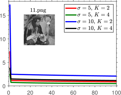
(a)

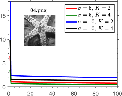
(b)

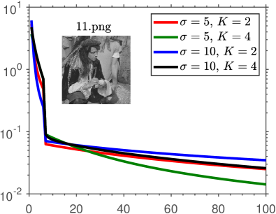
(c)

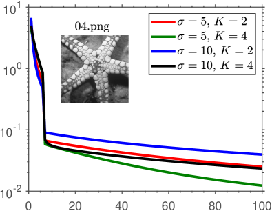
(d)

Figure 2: Objective and residual convergence for PnP-ISTA in $(\mathbb{R}^{n},\left\langle\cdot,\cdot\right\rangle)$ for $\rho=2.5$. Top row: $f(\boldsymbol{y}_{k})+\rho g_{D}(\boldsymbol{y}_{k})$. Bottom row: $\left\lVert\boldsymbol{x}_{k+1}-\boldsymbol{x}_{k}\right\rVert_{2}$ (on a logarithmic scale).

In Table I, we report PSNR/SSIM values, averaged over the images (resized to $256\times 256$) in the Set12 dataset [46]. Note that the reconstruction quality using PnP-ISTA in $(\mathbb{R}^{n},\left\langle\cdot,\cdot\right\rangle)$ is competitive with its standard counterpart. In particular, we note that this behavior holds for different values of $K$ and $\sigma$. For completeness, a visual result is shown in Fig. 1. We empirically verify Theorem III.9 for two particular images from the Set12 dataset and using different values of $K$ and $\sigma$; the results are reported in Fig. 2. Notice that the objective value corresponding to proposed algorithm decreases in every iteration and stabilizes. As for the iterates $(\boldsymbol{x}_{k})$, it is not possible to directly verify the convergence since the limit point $\boldsymbol{x}^{\ast}$ is not known. Instead, as shown in the figure, we verify a necessary condition, namely that $\left\lVert\boldsymbol{x}_{k}-\boldsymbol{x}_{k-1}\right\rVert_{2}$ decays to $0$ as $k$ increases.

IV-B Despeckling

TABLE II: Objective and iterate convergence of PnP-ADMM in $(\mathbb{R}^{n},\left\langle\cdot,\cdot\right\rangle)$ for image despeckling ($\rho=0.2$).

Image Settings $f(\boldsymbol{y}_{k})+\rho g_{D}(\boldsymbol{y}_{k})-C$ $\left\lVert\boldsymbol{y}_{k+1}-\boldsymbol{y}_{k}\right\rVert_{2}$ $k=1$ $k=10$ $k=20$ $k=30$ $k=40$ $C$ $k=1$ $k=10$ $k=20$ $k=30$ $k=40$ 03.png $M=5$ $1.8\times 10^{3}$ $2.7$ $1.6\times 10^{-2}$ $1.9\times 10^{-4}$ $3\times 10^{-6}$ $3.4\times 10^{6}$ $7.5\times 10^{1}$ $2.6\times 10^{-1}$ $1.3\times 10^{-2}$ $1.2\times 10^{-3}$ $1.4\times 10^{-4}$ $M=7$ $2.7\times 10^{3}$ $8.4$ $1.1\times 10^{-1}$ $2.6\times 10^{-3}$ $8.9\times 10^{-5}$ $4.7\times 10^{6}$ $6.7\times 10^{1}$ $3.2\times 10^{-1}$ $2.4\times 10^{-2}$ $3.1\times 10^{-3}$ $5.1\times 10^{-4}$ $M=10$ $4.1\times 10^{3}$ $2.4\times 10^{1}$ $5.9\times 10^{-1}$ $2.6\times 10^{-2}$ $1.7\times 10^{-3}$ $6.8\times 10^{6}$ $6.3\times 10^{1}$ $3.9\times 10^{-1}$ $4.2\times 10^{-2}$ $7.3\times 10^{-3}$ $1.6\times 10^{-3}$ 05.png $M=5$ $2.8\times 10^{3}$ $3.9$ $1.8\times 10^{-2}$ $1.6\times 10^{-4}$ $2.0\times 10^{-6}$ $3.3\times 10^{6}$ $8.0\times 10^{1}$ $3.1\times 10^{-1}$ $1.4\times 10^{-2}$ $1.1\times 10^{-3}$ $1.1\times 10^{-4}$ $M=7$ $4.1\times 10^{3}$ $1.2\times 10^{1}$ $1.2\times 10^{-1}$ $2.1\times 10^{-3}$ $5.1\times 10^{-5}$ $4.7\times 10^{6}$ $7.1\times 10^{1}$ $3.9\times 10^{-1}$ $2.7\times 10^{-2}$ $3.0\times 10^{-3}$ $4.1\times 10^{-4}$ $M=10$ $6.2\times 10^{3}$ $3.5\times 10^{1}$ $6.6\times 10^{-1}$ $2.0\times 10^{-2}$ $8.2\times 10^{-4}$ $6.7\times 10^{6}$ $6.6\times 10^{1}$ $4.9\times 10^{-1}$ $4.8\times 10^{-2}$ $7.1\times 10^{-3}$ $1.3\times 10^{-3}$

In $M$-look synthetic aperture radar imaging [58], the observation model is given by

$$\boldsymbol{s}(\boldsymbol{i})=\boldsymbol{r}_{0}(\boldsymbol{i})\boldsymbol{n}(\boldsymbol{i}),$$ (17)

where $\boldsymbol{i}$ is the pixel location, $\boldsymbol{r}_{0}\in\mathbb{R}_{++}^{n}$ is the unknown reflectance image, and the components of $\boldsymbol{n}\in\mathbb{R}_{+}^{n}$ (known as speckle noise) are i.i.d. Gamma with unit mean and variance $1/M$. In particular, the probability density of each component is

$$p_{n}(t)=\frac{M^{M}}{\Gamma(M)}t^{M-1}\exp(-Mt)\qquad(t\geqslant 0).$$

The above model is based on the assumption that the measurement $\boldsymbol{s}(\boldsymbol{i})$ is an average of $M$ independent samples of the intensity at pixel $\boldsymbol{i}$ [58]. Letting $\tilde{\boldsymbol{x}}(\boldsymbol{i})=\log\boldsymbol{r}_{0}(\boldsymbol{i})$ and $\boldsymbol{y}(\boldsymbol{i})=\log\boldsymbol{s}(\boldsymbol{i})$, and taking logarithms on both sides of (17), we obtain the following additive model:

$$\boldsymbol{y}(\boldsymbol{i})=\tilde{\boldsymbol{x}}(\boldsymbol{i})+\log\boldsymbol{n}(\boldsymbol{i}).$$

The transformed noise distribution is given by

$$p_{\log(n)}(t)=\frac{M^{M}}{\Gamma(M)}\exp\left(M(t-e^{t})\right).$$

The data-fidelity term corresponding to the maximum likelihood estimate of $\tilde{\boldsymbol{x}}$ is given by [8]:

$$f(\boldsymbol{x})=M\sum_{\boldsymbol{i}}\Big{(}\boldsymbol{x}(\boldsymbol{i})+\exp\big{(}\boldsymbol{y}(\boldsymbol{i})-\boldsymbol{x}(\boldsymbol{i})\big{)}\Big{)}+\text{constant}.$$

=Ground truth. =Observed. PSNR = $28.77$ dB.PnP, $(\mathbb{R}^{n},\left\langle\cdot,\cdot\right\rangle_{2})$. PSNR = $28.72$ dB.PnP, $(\mathbb{R}^{n},\left\langle\cdot,\cdot\right\rangle)$.

Figure 3: Image despeckling for $M=5$ using PnP-ADMM. The third and fourth images are the reconstructions from PnP-ADMM in $(\mathbb{R}^{n},\left\langle\cdot,\cdot\right\rangle_{2})$ and $(\mathbb{R}^{n},\left\langle\cdot,\cdot\right\rangle)$. The respective SSIM values are $0.840$ and $0.847$, while the PSNR values are reported above the images.

We use PnP-ADMM to estimate $\tilde{\boldsymbol{x}}$ using the above $f$ as the data-fidelity. Note that the proximal operator of $f$ in the space $(\mathbb{R}^{n},\left\langle\cdot,\cdot\right\rangle)$ is given by:

$$\mathrm{Prox}_{{\rho}^{-1}f}(\boldsymbol{u})= \operatorname*{\arg\!\min}_{\boldsymbol{x}\in\mathbb{R}^{n}}\bigg{\{}M\sum_{\boldsymbol{i}}\Big{[}\boldsymbol{x}(\boldsymbol{i})+\exp\big{(}\boldsymbol{y}(\boldsymbol{i})-\boldsymbol{x}(\boldsymbol{i})\big{)}\Big{]}$$

$$+\frac{\rho}{2}\left(\boldsymbol{x}-\boldsymbol{u}\right)^{\top}\!\mathbf{D}\left(\boldsymbol{x}-\boldsymbol{u}\right)\bigg{\}}.$$

The above optimization is separable since $\mathbf{D}$ is diagonal. In fact, the optimization can be decoupled into one-variable convex problems, which can be solved efficiently using Newton’s method [8].

A visual example of despeckling of a simulated observation is shown in Fig. 3 for $M=5$. The values of $f(\boldsymbol{y}_{k})+\rho g_{D}(\boldsymbol{y}_{k})$ and $\left\lVert\boldsymbol{y}_{k+1}-\boldsymbol{y}_{k}\right\rVert_{2}$ for different values of $M$ and input images are reported in Table II. It is evident that $f(\boldsymbol{y}_{k})+\rho g_{D}(\boldsymbol{y}_{k})$ converges to a stable value, whereas $\left\lVert\boldsymbol{y}_{k+1}-\boldsymbol{y}_{k}\right\rVert_{2}$ decays to $0$ with iterations $k$. These observations agree with Theorem III.10. We compare the reconstruction quality with PnP-ADMM in $(\mathbb{R}^{n},\left\langle\cdot,\cdot\right\rangle_{2})$ by averaging the PSNR and SSIM values over the images in the Set12 dataset (all images were resized to $256\times 256$). These are reported in Table III. Note that the PSNR/SSIM values are comparable for PnP-ADMM in $(\mathbb{R}^{n},\left\langle\cdot,\cdot\right\rangle)$ and $(\mathbb{R}^{n},\left\langle\cdot,\cdot\right\rangle_{2})$.

TABLE III: PSNR/SSIM values for despeckling of Set12 dataset [46] using PnP-ADMM.

	PnP in $(\mathbb{R}^{n},\left\langle\cdot,\cdot\right\rangle_{2})$	PnP in $(\mathbb{R}^{n},\left\langle\cdot,\cdot\right\rangle)$
$M=5$	$27.65/0.809$	$27.49/0.793$
$M=10$	$29.37/0.838$	$29.01/0.829$

V Conclusion

We showed that iterate and objective convergence of PnP-ISTA and PnP-ADMM can be guaranteed for a class of linear denoisers provided we work with a denoiser-specific inner product (and associated gradient and proximal operators). To the best of our knowledge, this is the first such result for PnP algorithms where simultaneous analysis of iterate and objective convergence can be carried out. Moreover, our results subsume existing convergence results for symmetric linear denoisers. Importantly, our analysis holds for non-symmetric kernel filters like nonlocal means which is known to possess good regularization capabilities. In fact, we demonstrated this for model-based superresolution and despeckling. An interesting question arising from our work is whether the present results (and analysis) can be extended to other proximal algorithms including the accelerated variants.

VI Appendix

In this section, we give detailed proofs of the results in Section III. Unless specified otherwise, it should be understood that we work in $(\mathbb{R}^{n},\left\langle\cdot,\cdot\right\rangle)$, where $\left\langle\cdot,\cdot\right\rangle$ is an arbitrary inner product and $\left\lVert\cdot\right\rVert$ denotes the norm induced by $\left\langle\cdot,\cdot\right\rangle$.

VI-A Proof of Proposition III.1

1) Let $\mathbf{A}=(1/\theta)\mathbf{W}-(1/\theta-1)\mathbf{I}$ and $\theta\in[1/2,1)$. Since the eigenvalues of $\mathbf{W}$ are in $[0,1]$, the eigenvalues of $\mathbf{A}$ must be in $[-1,1]$. Since $\mathbf{A}$ is symmetric, this means that its spectral norm $\left\lVert\mathbf{A}\right\rVert_{2}$ (largest singular value) is at most $1$. Hence, $\left\lVert\mathbf{A}(\boldsymbol{x}-\boldsymbol{y})\right\rVert_{2}\leqslant\left\lVert\mathbf{A}\right\rVert_{2}\left\lVert\boldsymbol{x}-\boldsymbol{y}\right\rVert_{2}\leqslant\left\lVert\boldsymbol{x}-\boldsymbol{y}\right\rVert_{2}$, i.e., $\mathbf{A}$ is non-expansive. Hence, $\mathbf{W}$ is $\theta$-averaged on $(\mathbb{R}^{n},\left\langle\cdot,\cdot\right\rangle_{2})$.

2) Since $\mathbf{W}$ is row-stochastic, $\mathbf{W}\boldsymbol{e}=\boldsymbol{e}$, where $\boldsymbol{e}\in\mathbb{R}^{n}$ is the all-ones vector. Thus, $1$ is an eigenvalue of $\mathbf{W}$. Since $\left\lVert\mathbf{W}\right\rVert_{2}=\max\{\left\lVert\mathbf{W}\boldsymbol{x}\right\rVert_{2}:\left\lVert\boldsymbol{x}\right\rVert_{2}=1\}$, we can conclude that

$$\left\lVert\mathbf{W}\right\rVert_{2}\geqslant 1.$$ (18)

Suppose that $D$ is averaged. Then we can show that $\mathbf{W}^{\top}\!\boldsymbol{e}=\boldsymbol{e}$. But this would contradict our assumption that $\mathbf{W}$ is not doubly stochastic, hence $D$ cannot be averaged. Indeed, if $D$ is averaged, then it is non-expansive: $\left\lVert\mathbf{W}\boldsymbol{x}\right\rVert_{2}\leqslant\left\lVert\boldsymbol{x}\right\rVert_{2}$ for all $\boldsymbol{x}\in\mathbb{R}^{n}$. Thus, we must have $\left\lVert\mathbf{W}\right\rVert_{2}\leqslant 1$. Hence, from (18), it follows that $\left\lVert\mathbf{W}\right\rVert_{2}=1$. Now, since $\left\lVert\mathbf{W}^{\top}\right\rVert_{2}=\left\lVert\mathbf{W}\right\rVert_{2}$,

$$\left\lVert\boldsymbol{e}\right\rVert_{2}^{2}={\boldsymbol{e}}^{\top}(\mathbf{W}\boldsymbol{e})={(\mathbf{W}^{\top}\boldsymbol{e}})^{\top}\!\boldsymbol{e} \leqslant\left\lVert\mathbf{W}^{\top}\boldsymbol{e}\right\rVert_{2}\left\lVert\boldsymbol{e}\right\rVert_{2}$$

$$\leqslant\left\lVert\mathbf{W}^{\top}\right\rVert_{2}\left\lVert\boldsymbol{e}\right\rVert_{2}^{2}=\left\lVert\boldsymbol{e}\right\rVert_{2}^{2}.$$

Thus, both “$\leqslant$” are in fact “$=$”. In particular, for the Cauchy-Schwarz inequality, we must have $\mathbf{W}^{\top}\!\boldsymbol{e}=\alpha\boldsymbol{e}$, where $\alpha\in\mathbb{R}$. However,

$$(\alpha{\boldsymbol{e}})^{\top}\boldsymbol{e}={(\mathbf{W}^{\top}\!\boldsymbol{e}})^{\top}\!\boldsymbol{e}={\boldsymbol{e}}^{\top}\!(\mathbf{W}\boldsymbol{e})={\boldsymbol{e}}^{\top}\boldsymbol{e}.$$

Hence, $\alpha=1$ and $\mathbf{W}^{\top}\!\boldsymbol{e}=\boldsymbol{e}$, as claimed.

VI-B Proof of Lemma III.3

To prove Lemma III.3, we need the following result. A proof can be found in [51, Proposition 4.35(iii)]. Nevertheless, we offer a more self-contained analysis.

Lemma VI.1

Let $T:\mathbb{R}^{n}\to\mathbb{R}^{n}$ be $\theta$-averaged for some $\theta\in(0,1)$. Then, for all $\boldsymbol{x},\boldsymbol{y}\in\mathbb{R}^{n}$,

$$\left\lVert T(\boldsymbol{x})-T(\boldsymbol{y})\right\rVert^{2}\leqslant \left\lVert\boldsymbol{x}-\boldsymbol{y}\right\rVert^{2}$$

$$-\frac{1-\theta}{\theta}\left\lVert(I-T)(\boldsymbol{x})-(I-T)(\boldsymbol{y})\right\rVert^{2}.$$

Proof:

Let $T=(1-\theta)I+\theta S$, where $S$ is non-expansive. Then $I-T=\theta(I-S)=\theta\Delta S$, where $\Delta S=I-S$. We need to show that for all $\boldsymbol{x},\boldsymbol{y}\in\mathbb{R}^{n}$,

$$\left\lVert T(\boldsymbol{x})-T(\boldsymbol{y})\right\rVert^{2}\leqslant\left\lVert\boldsymbol{x}-\boldsymbol{y}\right\rVert^{2}-\theta(1-\theta)\left\lVert\Delta S(\boldsymbol{x})-\Delta S(\boldsymbol{y})\right\rVert^{2}.$$

Now $T(\boldsymbol{x})-T(\boldsymbol{y})=(\boldsymbol{x}-\boldsymbol{y})-\theta\big{(}\Delta S(\boldsymbol{x})-\Delta S(\boldsymbol{y})\big{)}$. Hence,

$$\quad\left\lVert T(\boldsymbol{x})-T(\boldsymbol{y})\right\rVert^{2}=$$

$$\left[\left\lVert\boldsymbol{x}-\boldsymbol{y}\right\rVert^{2}-\theta(1-\theta)\left\lVert\Delta S(\boldsymbol{x})-\Delta S(\boldsymbol{y})\right\rVert^{2}\right]$$

$$+ \left[\theta\left\lVert\Delta S(\boldsymbol{x})-\Delta S(\boldsymbol{y})\right\rVert^{2}-2\theta\left\langle\boldsymbol{x}-\boldsymbol{y},\Delta S(\boldsymbol{x})-\Delta S(\boldsymbol{y})\right\rangle\right].$$

It suffices to show that the second term on the right is negative. Indeed, note that

$$\left\lVert\Delta S(\boldsymbol{x})-\Delta S(\boldsymbol{y})\right\rVert^{2}-2\left\langle\boldsymbol{x}-\boldsymbol{y},\Delta S(\boldsymbol{x})-\Delta S(\boldsymbol{y})\right\rangle$$

$$= \left\langle\Delta S(\boldsymbol{x})-\Delta S(\boldsymbol{y}),\Delta S(\boldsymbol{x})-\Delta S(\boldsymbol{y})-2(\boldsymbol{x}-\boldsymbol{y})\right\rangle$$

$$= \left\langle\boldsymbol{x}-\boldsymbol{y}-S(\boldsymbol{x})+S(\boldsymbol{y}),-\boldsymbol{x}+\boldsymbol{y}-S(\boldsymbol{x})+S(\boldsymbol{y})\right\rangle$$

$$= \left\lVert S(\boldsymbol{y})-S(\boldsymbol{x})\right\rVert^{2}-\left\lVert\boldsymbol{y}-\boldsymbol{x}\right\rVert^{2}\leqslant 0,$$

since $S$ is non-expansive. ∎

We now establish Lemma III.3 using the above result. Letting $S=I-T$, note that $\boldsymbol{x}_{\ast}\in\mathrm{fix}(T)$ if and only if $S(\boldsymbol{x}_{\ast})=\mathbf{0}$. Since by assumption $\mathrm{fix}(T)\neq\varnothing$, let $\boldsymbol{x}_{\ast}\in\mathrm{fix}(T)$. Setting $\boldsymbol{x}=\boldsymbol{x}_{k}$ and $\boldsymbol{y}=\boldsymbol{x}_{\ast}$ in Lemma VI.1, we have

$$\left\lVert\boldsymbol{x}_{k+1}-\boldsymbol{x}_{\ast}\right\rVert^{2}\leqslant\left\lVert\boldsymbol{x}_{k}-\boldsymbol{x}_{\ast}\right\rVert^{2}-\frac{1-\theta}{\theta}\left\lVert S(\boldsymbol{x}_{k})\right\rVert^{2},$$ (19)

since $S(\boldsymbol{x}_{\ast})=\boldsymbol{0}$. By telescoping the sum in (19), we obtain

$$\left\lVert\boldsymbol{x}_{k+1}-\boldsymbol{x}_{\ast}\right\rVert^{2}\leqslant\left\lVert\boldsymbol{x}_{0}-\boldsymbol{x}_{\ast}\right\rVert^{2}-\frac{1-\theta}{\theta}\sum_{j=0}^{k}\left\lVert S(\boldsymbol{x}_{j})\right\rVert^{2}.$$

The quantity on the right is nonnegative for all $k\geqslant 1$. In particular, the series $\sum_{j=0}^{\infty}\left\lVert S(\boldsymbol{x}_{j})\right\rVert^{2}$ is bounded above by $\left\lVert\boldsymbol{x}_{0}-\boldsymbol{x}_{\ast}\right\rVert^{2}$. Thus, we must have $S(\boldsymbol{x}_{k})\rightarrow\mathbf{0}$ as $k\rightarrow\infty$.

On the other hand, it follows from (19) that

$$\left\lVert\boldsymbol{x}_{k+1}-\boldsymbol{x}_{\ast}\right\rVert\leqslant\left\lVert\boldsymbol{x}_{k}-\boldsymbol{x}_{\ast}\right\rVert\leqslant\cdots\leqslant\left\lVert\boldsymbol{x}_{0}-\boldsymbol{x}_{\ast}\right\rVert.$$ (20)

We conclude that $(\boldsymbol{x}_{k})_{k\geqslant 0}$ is bounded and thus must have a convergent subsequence, i.e., a subsequence $(\boldsymbol{x}_{k_{r}})_{r\geqslant 0}$ that converges to some $\hat{\boldsymbol{x}}\in\mathbb{R}^{n}$. Since $S$ is continuous, we have

$$S(\hat{\boldsymbol{x}})=\lim_{r\rightarrow\infty}S(\boldsymbol{x}_{k_{r}})=\lim_{k\rightarrow\infty}S(\boldsymbol{x}_{k})=\mathbf{0},$$

Hence, $\hat{\boldsymbol{x}}\in\mathrm{fix}(T)$.

We are done if we can show that the original sequence $(\boldsymbol{x}_{k})_{k\geqslant 0}$ converges to $\hat{\boldsymbol{x}}$. Now, given any $\epsilon>0$, we can find $N\geqslant 1$ such that $\left\lVert\boldsymbol{x}_{k_{n}}-\hat{\boldsymbol{x}}\right\rVert<\epsilon$ for $n\geqslant N$. Let $K=k_{N}$. Since $\hat{\boldsymbol{x}}\in\mathrm{fix}(T)$, it follows from (20) that for $k\geqslant K$,

$$\left\lVert\boldsymbol{x}_{k}-\hat{\boldsymbol{x}}\right\rVert\leqslant\left\lVert\boldsymbol{x}_{k_{N}}-\hat{\boldsymbol{x}}\right\rVert<\epsilon.$$

Since $\epsilon$ is arbitrary, we conclude that $\boldsymbol{x}_{k}\rightarrow\hat{\boldsymbol{x}}$ as $k\rightarrow\infty$.

VI-C Proof of Theorem III.5

We need some preliminary results to establish Theorem III.5.

Lemma VI.2

Let $f:\mathbb{R}^{n}\to\mathbb{R}$ be convex and $\beta$-smooth. Then, for any $\boldsymbol{x},\boldsymbol{y}\in\mathbb{R}^{n}$,

$$\left\langle\nabla\!f(\boldsymbol{x})-\nabla\!f(\boldsymbol{y}),\boldsymbol{x}-\boldsymbol{y}\right\rangle\geqslant\frac{1}{\beta}\left\lVert\nabla\!f(\boldsymbol{x})-\nabla\!f(\boldsymbol{y})\right\rVert^{2}.$$

Proof:

See [59, Theorem 2.1.5]. ∎

Lemma VI.3

Let $f:\mathbb{R}^{n}\to\mathbb{R}$ be convex and $\beta$-smooth. Then the operator $(I-\rho^{-1}\nabla\!f)$ is $(\beta/2\rho)$-averaged for $\rho>\beta/2$.

Proof:

Let $\theta=\beta/2\rho\in(0,1)$, and let $S=I-(2/\beta)\nabla\!f$. Then $I-\rho^{-1}\nabla\!f=(1-\theta)I+\theta S$. We are done if we can show that $S$ is non-expansive. Indeed, for any $\boldsymbol{x},\boldsymbol{y}\in\mathbb{R}^{n}$,

$$\left\lVert S(\boldsymbol{x})-S(\boldsymbol{y})\right\rVert^{2}=\left\lVert(\boldsymbol{x}-\boldsymbol{y})-\frac{2}{\beta}\big{(}\nabla\!f(\boldsymbol{x})-\nabla\!f(\boldsymbol{y})\big{)}\right\rVert^{2}$$

$$=\left\lVert\boldsymbol{x}-\boldsymbol{y}\right\rVert^{2}+\frac{4}{\beta}\Big{[}\frac{1}{\beta}\left\lVert\nabla\!f(\boldsymbol{x})-\nabla\!f(\boldsymbol{y})\right\rVert^{2}$$

$$\qquad\qquad\qquad\qquad-\left\langle\boldsymbol{x}-\boldsymbol{y},\nabla\!f(\boldsymbol{x})-\nabla\!f(\boldsymbol{y})\right\rangle\Big{]}$$

$$\leqslant\left\lVert\boldsymbol{x}-\boldsymbol{y}\right\rVert^{2},$$

where the last inequality follows from Lemma VI.2. ∎

Lemma VI.4

If $T_{1},T_{2}:\mathbb{R}^{n}\to\mathbb{R}^{n}$ are averaged, then $T_{1}\circ T_{2}$ is averaged.

Proof:

See [51, Proposition 4.44]. ∎

We are now ready to prove Theorem III.5. By Lemma VI.3, $(I-\rho^{-1}\nabla\!f)$ is averaged if $\rho>\beta/2$. Since $D$ is assumed to be averaged, it follows from Lemma VI.4 that $T_{\mathrm{ISTA}}$ is averaged if $\rho>\beta/2$. Finally, since $\mathrm{fix}(T_{\mathrm{ISTA}})\neq\varnothing$, Theorem III.5 follows immediately from Lemma III.3.

VI-D Proof of Theorem III.6

We first show that the PnP-ADMM iterates $(\boldsymbol{x}_{k},\boldsymbol{y}_{k},\boldsymbol{z}_{k})_{k\geqslant 1}$ can be written in terms of a single-variable sequence $(\boldsymbol{u}_{k})_{k\geqslant 1}$.

Lemma VI.5

Fix $\rho>0$ and $\boldsymbol{y}_{0},\boldsymbol{z}_{0}\in\mathbb{R}^{n}$, and consider the sequence $(\boldsymbol{x}_{k},\boldsymbol{y}_{k},\boldsymbol{z}_{k})_{k\geqslant 1}$ generated by (6). Let $\boldsymbol{u}_{1}=\boldsymbol{y}_{1}+\boldsymbol{z}_{1}$, and $\boldsymbol{u}_{k}=T_{\mathrm{ADMM}}(\boldsymbol{u}_{k-1})$ for $k\geqslant 2$, where $T_{\mathrm{ADMM}}$ is given by (7). Then for $k\geqslant 1$, we have $\boldsymbol{y}_{k}=D(\boldsymbol{u}_{k}),\ \boldsymbol{z}_{k}=(I-D)(\boldsymbol{u}_{k})$ and $\boldsymbol{x}_{k+1}=\mathrm{Prox}_{\rho^{-1}f}\circ(2D-I)(\boldsymbol{u}_{k})$.

Proof:

Define $\hat{\boldsymbol{y}}_{k}=D(\boldsymbol{u}_{k}),\hat{\boldsymbol{z}}_{k}=(I-D)(\boldsymbol{u}_{k}),$ and $\hat{\boldsymbol{x}}_{k+1}=\mathrm{Prox}_{\rho^{-1}f}\circ(2D-I)(\boldsymbol{u}_{k})$. We will inductively show that for $i\geqslant 1$,

$$\boldsymbol{y}_{i}=\hat{\boldsymbol{y}}_{i},\ \boldsymbol{z}_{i}=\hat{\boldsymbol{z}}_{i}\text{ and }\boldsymbol{x}_{i+1}=\hat{\boldsymbol{x}}_{i+1}.$$ (21)

Base case: First, note that (21) holds for $i=1$. Indeed, from (6b) and (6c), we have $\boldsymbol{y}_{1}=D(\boldsymbol{x}_{1}+\boldsymbol{z}_{0})$ and $\boldsymbol{z}_{1}=\boldsymbol{z}_{0}+\boldsymbol{x}_{1}-\boldsymbol{y}_{1}$. Since, by construction, $\boldsymbol{u}_{1}=\boldsymbol{y}_{1}+\boldsymbol{z}_{1}$, we have $\boldsymbol{u}_{1}=\boldsymbol{z}_{0}+\boldsymbol{x}_{1}$. Therefore, $\boldsymbol{y}_{1}=D(\boldsymbol{x}_{1}+\boldsymbol{z}_{0})=D(\boldsymbol{u}_{1})=\hat{\boldsymbol{y}}_{1}$, and

$$\boldsymbol{z}_{1}=\boldsymbol{u}_{1}-\boldsymbol{y}_{1}=\boldsymbol{u}_{1}-D(\boldsymbol{u}_{1})=(I-D)(\boldsymbol{u}_{1})=\hat{\boldsymbol{z}}_{1}.$$

Moreover, $\boldsymbol{y}_{1}-\boldsymbol{z}_{1}=(2D-I)(\boldsymbol{u}_{1})$. Hence, from (6a), we get that $\boldsymbol{x}_{2}=\mathrm{Prox}_{\rho^{-1}f}\circ(2D-I)(\boldsymbol{u}_{1})=\hat{\boldsymbol{x}}_{2}$.

Induction: Assume that (21) holds for $1\leqslant i\leqslant k-1$. We need to show that (21) holds for $i=k$. From the definition of $T_{\mathrm{ADMM}}$ and the induction hypothesis, we have

$$\boldsymbol{u}_{k} =T_{\mathrm{ADMM}}(\boldsymbol{u}_{k-1})$$

$$=\mathrm{Prox}_{\rho^{-1}f}\circ(2D-I)(\boldsymbol{u}_{k-1})+(I-D)(\boldsymbol{u}_{k-1})$$

$$=\hat{\boldsymbol{x}}_{k}+\hat{\boldsymbol{z}}_{k-1}$$

$$=\boldsymbol{x}_{k}+\boldsymbol{z}_{k-1}.$$

Using (6b), (6c) and the induction hypothesis, we see that

$$\hat{\boldsymbol{y}}_{k}=D(\boldsymbol{u}_{k})=D(\boldsymbol{x}_{k}+\boldsymbol{z}_{k-1})=\boldsymbol{y}_{k},$$

and

$$\hat{\boldsymbol{z}}_{k}=(I-D)(\boldsymbol{u}_{k})=\boldsymbol{u}_{k}-\hat{\boldsymbol{y}}_{k}=\boldsymbol{z}_{k-1}+\boldsymbol{x}_{k}-\boldsymbol{y}_{k}=\boldsymbol{z}_{k}.$$

Finally, note that $(2D-I)(\boldsymbol{u}_{k})=\boldsymbol{y}_{k}-\boldsymbol{z}_{k}$. Thus, from (6a) and the definition of $\hat{\boldsymbol{x}}_{k+1}$, we have

$$\hat{\boldsymbol{x}}_{k+1}=\mathrm{Prox}_{\rho^{-1}f}(\boldsymbol{y}_{k}-\boldsymbol{z}_{k})=\boldsymbol{x}_{k+1}.$$

This completes the induction and the proof of Lemma VI.5. ∎

Next, we need a standard result about proximal operators.

Lemma VI.6

Let $f:\mathbb{R}^{n}\to\overline{\mathbb{R}}$ be closed, proper and convex. Then $\mathrm{Prox}_{f}$ is $(1/2)$-averaged.

Proof:

See [51, Proposition 2.28, Proposition 4.4]. ∎

Finally, we need the following property of averaged operators.

Lemma VI.7

If $T:\mathbb{R}^{n}\to\mathbb{R}^{n}$ is $\theta$-averaged, then $T$ is $\bar{\theta}$-averaged for all $\bar{\theta}\in[\theta,1)$.

Proof:

Let $T=(1-\theta)I+\theta S$, where $\theta\in(0,1)$ and $S$ is non-expansive. Fix $\bar{\theta}\in[\theta,1)$ and define $\gamma=\theta/\bar{\theta}$. Then $T=(1-\bar{\theta})I+\bar{\theta}\bar{S}$, where $\bar{S}=(1-\gamma)I+\gamma S$. Since $\bar{S}$ is non-expansive by triangle inequality and $\bar{\theta}\in[\theta,1)$ was arbitrary, it follows that $T$ is averaged for all $\bar{\theta}\in[\theta,1)$. ∎

Using the above results, we can now establish Theorem III.6. Note that:

• $2\mathrm{Prox}_{\rho^{-1}f}-I$ is non-expansive since $\mathrm{Prox}_{\rho^{-1}f}$ is $(1/2)$-averaged (Lemma VI.6).

• $2D-I$ is non-expansive since $D$ is $(1/2)$-averaged by Lemma VI.7.

• Thus, $(2\mathrm{Prox}_{\rho^{-1}f}-I)\circ(2D-I)$ is non-expansive. Hence, $T_{\mathrm{ADMM}}$ is $(1/2)$-averaged.

• Since $\mathrm{fix}(T_{\mathrm{ADMM}})\neq\varnothing$, Lemma III.3 implies that the sequence ${(\boldsymbol{u}_{k})}_{k\geqslant 1}$ in Proposition VI.5 converges to some $\boldsymbol{u}^{\ast}\in\mathrm{fix}(T_{\mathrm{ADMM}})$.

• Since $D$ and $\mathrm{Prox}_{\rho^{-1}f}$ are continuous, we have

  $$\boldsymbol{x}_{k} \longrightarrow\mathrm{Prox}_{{\rho}^{-1}f}\circ\left(2D-I\right)(\boldsymbol{u}^{\ast}),$$

  $$\boldsymbol{y}_{k} \longrightarrow D(\boldsymbol{u}^{\ast})\ \text{ and }\ \boldsymbol{z}_{k}\longrightarrow(I-D)(\boldsymbol{u}^{\ast}).$$

This completes the proof of Theorem III.6.

VI-E Proof of Theorem III.8

(a) We use the following result from [60, Corollary 3.4]: A linear operator $D$ on $(\mathbb{R}^{n},\left\langle\cdot,\cdot\right\rangle)$ is the proximal operator of a closed proper convex function if the following conditions are met: (i) $D$ is self-adjoint; (ii) $\left\langle\boldsymbol{x},D(\boldsymbol{x})\right\rangle\geqslant 0$ for all $\boldsymbol{x}\in\mathbb{R}^{n}$; and (iii) $\left\lVert D\right\rVert\leqslant 1$, where $\left\lVert D\right\rVert$ is the operator norm of $D$.

We verify that the above three conditions are satisfied by any $D\in\mathcal{L}$. Let $\mathbf{W}=\mathbf{V}\mathbf{A}\mathbf{V}^{-1}$ be an eigendecomposition of $\mathbf{W}$, where the diagonal matrix $\mathbf{A}$ contains the eigenvalues of $\mathbf{W}$ For (i), we need to show that $\left\langle\boldsymbol{x},D(\boldsymbol{y})\right\rangle=\left\langle D(\boldsymbol{x}),\boldsymbol{y}\right\rangle$ for all $\boldsymbol{x},\boldsymbol{y}\in\mathbb{R}^{n}$. This is straightforward from definition (8) by writing $\mathbf{W}=\mathbf{V}\mathbf{A}\mathbf{V}^{-1}$. Similarly, (ii) follows using the fact that the entries of $\mathbf{A}$ are nonnegative. To prove (iii), note that by definition $\left\lVert D\right\rVert=\max\{\left\lVert\mathbf{W}\boldsymbol{x}\right\rVert:\left\lVert\boldsymbol{x}\right\rVert=1\}$. Let $\boldsymbol{y}=\mathbf{V}^{-1}\boldsymbol{x}$. Then $\left\lVert\boldsymbol{x}\right\rVert=\left\lVert\boldsymbol{y}\right\rVert_{2}$. Moreover, since $\mathbf{W}=\mathbf{V}\mathbf{A}\mathbf{V}^{-1}$, we have $\left\lVert\mathbf{W}\boldsymbol{x}\right\rVert=\left\lVert\mathbf{A}\boldsymbol{y}\right\rVert_{2}$. Hence,

$$\left\lVert D\right\rVert=\max\left\{\left\lVert\mathbf{A}\boldsymbol{y}\right\rVert_{2}:\left\lVert\boldsymbol{y}\right\rVert_{2}=1\right\}\leqslant 1,$$

since the diagonal entries of $\mathbf{A}$ are in $[0,1]$.

(b) From part (a), we have

$$\mathbf{W}\boldsymbol{x}=\mathrm{Prox}_{g_{D}}(\boldsymbol{x}),\qquad(\boldsymbol{x}\in\mathbb{R}^{n})$$ (22)

where $g_{D}:\mathbb{R}^{n}\to\overline{\mathbb{R}}$ is closed proper and convex. Hence (b) follows from Lemma VI.6 and Lemma VI.7.

(c) From (22), $\mathrm{Prox}_{g_{D}}$ maps $\mathbb{R}^{n}$ onto $\mathcal{R}(\mathbf{W})$. Moreover, since $g_{D}$ is proper and from (22), $g_{D}$ is real-valued on $\mathcal{R}(\mathbf{W})$. To prove that $g_{D}$ restricted to $\mathcal{R}(\mathbf{W})$ is continuous, note that $\mathcal{R}(\mathbf{W})$ is a subspace of $\mathbb{R}^{n}$. If $\dim\mathcal{R}(\mathbf{W})=0$, then continuity follows trivially. Hence, assume that $\dim\mathcal{R}(\mathbf{W})=p\geqslant 1$. Let $\varphi:\mathbb{R}^{p}\to\mathcal{R}(\mathbf{W})$ be a linear isomorphism, and define $h=g_{D}\circ\varphi$. Since $g_{D}$ is convex and $\varphi$ is linear, $h$ is convex. Since real-valued convex functions are continuous (see [51, Corollary 8.40]), $h$ is continuous. Further, since $\varphi^{-1}$ is continuous, it follows that $g_{D}|_{\mathcal{R}(\mathbf{W})}=h\circ\varphi^{-1}$ is continuous.

(d) Since $D=\mathrm{Prox}_{g_{D}}$, we can replace the denoiser $D$ by $\mathrm{Prox}_{g_{D}}$ in (5) and (6b). Then, the updates in PnP-ISTA (resp. PnP-ADMM) are exactly that of ISTA (resp. ADMM) applied to optimization problem (9).

VI-F Proof of Theorem III.9

To establish this theorem, we will require the concept of subdifferential of a convex function.

Definition VI.8

Let $f:\mathbb{R}^{n}\to\overline{\mathbb{R}}$ be proper and convex. The subdifferential of $f$ at $\boldsymbol{x}\in\mathbb{R}^{n}$, denoted by $\partial f(\boldsymbol{x})$, is defined to be the set of all vectors $\boldsymbol{v}\in\mathbb{R}^{n}$ such that

$$f(\boldsymbol{y})\geqslant f(\boldsymbol{x})+\left\langle\boldsymbol{v},\boldsymbol{y}-\boldsymbol{x}\right\rangle\qquad(\boldsymbol{y}\in\mathbb{R}^{n}).$$

As with the rest of the discussion, we assume $\left\langle\cdot,\cdot\right\rangle$ to be an arbitrary (but fixed) inner product on $\mathbb{R}^{n}$.

We need the following properties of subdifferential.

Lemma VI.9

Let $f:\mathbb{R}^{n}\to\mathbb{R}$ be convex and $g:\mathbb{R}^{n}\to\overline{\mathbb{R}}$ be closed proper and convex. Then

1. $\boldsymbol{x}^{\ast}$ minimizes $h(\boldsymbol{x})=g(\boldsymbol{x})+(\rho/2)\left\lVert\boldsymbol{x}-\bar{\boldsymbol{x}}\right\rVert^{2}$, where $\rho>0$ and $\bar{\boldsymbol{x}}\in\mathbb{R}^{n}$, if and only if $\mathbf{0}\in\partial g(\boldsymbol{x}^{\ast})+\rho(\boldsymbol{x}^{\ast}-\bar{\boldsymbol{x}})$.

2. $\boldsymbol{x}^{\ast}$ minimizes $f+g$ if and only if $\mathbf{0}\in\partial f(\boldsymbol{x}^{\ast})+\partial g(\boldsymbol{x}^{\ast})$. If $f$ is differentiable, then $\mathbf{0}\in\nabla\!f(\boldsymbol{x}^{\ast})+\partial g(\boldsymbol{x}^{\ast})$.

Proof:

For (a), see [51, Th. 16.3 and Example 16.43]. For (b), see [51, Th. 16.3 and Corollary 16.48]. ∎

Proposition VI.10

Let $f:\mathbb{R}^{n}\to\mathbb{R}$ be convex and differentiable, and let $g:\mathbb{R}^{n}\to\overline{\mathbb{R}}$ be closed proper and convex. Then $\boldsymbol{x}^{\ast}\in\mathrm{fix}({T}_{\mathrm{ISTA}})$ where $D=\mathrm{Prox}_{\rho^{-1}g}$ if and only if $\boldsymbol{x}^{\ast}$ is a minimizer of $f+g$.

Proof:

Let $\boldsymbol{x}^{\ast}\in\mathrm{fix}(T_{\mathrm{ISTA}})$, where $T_{\mathrm{ISTA}}=\mathrm{Prox}_{{\rho^{-1}}g}\circ(I-\rho^{-1}\nabla\!f)$. Let $\boldsymbol{y}^{\ast}=(I-\rho^{-1}\nabla\!f)(\boldsymbol{x}^{\ast})$. Then $\nabla f(\boldsymbol{x}^{\ast})=\rho(\boldsymbol{x}^{\ast}-\boldsymbol{y}^{\ast})$. Moreover,

$$\boldsymbol{x}^{\ast}=T_{\mathrm{ISTA}}(\boldsymbol{x}^{\ast})=\mathrm{Prox}_{{\rho^{-1}}g}(\boldsymbol{y}^{\ast}).$$

That is,

$$\boldsymbol{x}^{\ast}=\operatorname*{\arg\!\min}_{\boldsymbol{y}\in\mathbb{R}^{n}}\ g(\boldsymbol{y})+\frac{\rho}{2}\left\lVert\boldsymbol{y}-\boldsymbol{y}^{\ast}\right\rVert^{2}.$$

Therefore, by Lemma VI.9, $\mathbf{0}\in\partial g(\boldsymbol{x}^{\ast})+\rho(\boldsymbol{x}^{\ast}-\boldsymbol{y}^{\ast})$. Thus,

$$\mathbf{0}\in\partial g(\boldsymbol{x}^{\ast})+\rho(\boldsymbol{x}^{\ast}-\boldsymbol{y}^{\ast})=\partial g(\boldsymbol{x}^{\ast})+\nabla\!f(\boldsymbol{x}^{\ast}).$$

Using Lemma VI.9, we conclude that $\boldsymbol{x}^{\ast}$ is a minimizer of $f+g$. The other direction can be established by reversing the above steps. ∎

Using the above results, we can now arrive at Theorem III.9. Note that since $D\in\mathcal{L}$, $D$ is averaged by Proposition III.8. Moreover, since (9) has a minimizer, $\mathrm{fix}(T_{\mathrm{ISTA}})\neq\varnothing$ by Proposition VI.10. Therefore, from Theorem III.5 and Proposition VI.10, we can conclude that ${(\boldsymbol{x}_{k})}_{k\geqslant 0}\to\boldsymbol{x}^{\ast}$, where $\boldsymbol{x}^{\ast}$ is a minimizer of (9). In particular, since $D=\mathrm{Prox}_{g_{D}}$,

$$p^{\ast}=f(\boldsymbol{x}^{\ast})+\rho g_{D}(\boldsymbol{x}^{\ast}).$$

Now, $\boldsymbol{x}^{\ast}\in\mathrm{fix}(T_{\mathrm{ISTA}})\subseteq\mathcal{R}(\mathbf{W})$ and $\boldsymbol{x}_{k}\in\mathcal{R}(\mathbf{W})$ for all $k$. On the other hand, $f$ is continuous on $\mathbb{R}^{n}$ and $g_{D}$ is continuous on $\mathcal{R}(\mathbf{W})$ by Theorem III.8. Therefore, by continuity, we have

$$f(\boldsymbol{x}_{k})+\rho g_{D}(\boldsymbol{x}_{k})\longrightarrow f(\boldsymbol{x}^{\ast})+\rho g_{D}(\boldsymbol{x}^{\ast})=p^{\ast}.$$

This completes the proof of Theorem III.9.

VI-G Proof of Theorem III.10

We first prove a result similar to Proposition VI.10 that relates $\mathrm{fix}(T_{\mathrm{ADMM}})$ to the minimizers of (9).

Proposition VI.11

Let $f:\mathbb{R}^{n}\to\mathbb{R}$ be convex and $g:\mathbb{R}^{n}\to\overline{\mathbb{R}}$ be closed, proper and convex. Then $\boldsymbol{x}^{\ast}\in\mathrm{fix}({T}_{\mathrm{ADMM}})$ with $D=\mathrm{Prox}_{\rho^{-1}g}$ if and only if $D(\boldsymbol{x}^{\ast})$ is a minimizer of $f+g$..

Proof:

Suppose $\boldsymbol{x}^{\ast}\in\mathrm{fix}(T_{\mathrm{ADMM}})$, i.e.,

$$\boldsymbol{x}^{\ast}=\left(2\mathrm{Prox}_{\rho^{-1}f}-I\right)\circ\left(2\mathrm{Prox}_{\rho^{-1}g}-I\right)(\boldsymbol{x}^{\ast}).$$

Let $\boldsymbol{y}^{\ast}=\left(2\mathrm{Prox}_{\rho^{-1}g}-I\right)(\boldsymbol{x}^{\ast})$. Note that

$$\mathrm{Prox}_{\rho^{-1}g}(\boldsymbol{x}^{\ast})=\frac{\boldsymbol{x}^{\ast}+\boldsymbol{y}^{\ast}}{2}=\mathrm{Prox}_{\rho^{-1}f}(\boldsymbol{y}^{\ast}).$$ (23)

From Lemma VI.9, we have

$$\mathbf{0} \in\partial g\Big{(}\frac{\boldsymbol{x}^{\ast}+\boldsymbol{y}^{\ast}}{2}\Big{)}+\frac{\rho}{2}(\boldsymbol{y}^{\ast}-\boldsymbol{x}^{\ast}),\ \text{and}$$

$$\mathbf{0} \in\partial f\Big{(}\frac{\boldsymbol{x}^{\ast}+\boldsymbol{y}^{\ast}}{2}\Big{)}+\frac{\rho}{2}(\boldsymbol{x}^{\ast}-\boldsymbol{y}^{\ast}).$$

Adding these inclusions and using (23), we obtain

$$\mathbf{0}\in\partial f\left(\mathrm{Prox}_{\rho^{-1}g}(\boldsymbol{x}^{\ast})\right)+\partial g\left(\mathrm{Prox}_{\rho^{-1}g}(\boldsymbol{x}^{\ast})\right).$$

Since $D=\mathrm{Prox}_{\rho^{-1}g}$, we conclude from Lemma VI.9 that $D(\boldsymbol{x}^{\ast})$ is a minimizer of $f+g$.

Conversely, let $\boldsymbol{y}^{\ast}=\mathrm{Prox}_{\rho^{-1}g}(\boldsymbol{x}^{\ast})$. From Lemma VI.9, we have $\mathbf{0}\in\partial g(\boldsymbol{y}^{\ast})+\rho(\boldsymbol{y}^{\ast}-\boldsymbol{x}^{\ast})$. Moreover, since $\boldsymbol{y}^{\ast}=D(\boldsymbol{x}^{\ast})$, $\boldsymbol{y}^{\ast}$ is a minimizer of $f+g$. Using Lemma VI.9 once more, we have $\mathbf{0}\in\partial f(\boldsymbol{y}^{\ast})+\partial g(\boldsymbol{y}^{\ast})$. Combining these, we obtain

$$\mathbf{0}\in\partial f(\boldsymbol{y}^{\ast})+\rho(\boldsymbol{x}^{\ast}-\boldsymbol{y}^{\ast}),$$

i.e., $\boldsymbol{y}^{\ast}=\mathrm{Prox}_{\rho^{-1}f}(2\boldsymbol{y}^{\ast}-\boldsymbol{x}^{\ast})$, or equivalently,

$$\boldsymbol{x}^{\ast}=\left(2\mathrm{Prox}_{\rho^{-1}f}-I\right)(2\boldsymbol{y}^{\ast}-\boldsymbol{x}^{\ast}).$$ (24)

However, $2\boldsymbol{y}^{\ast}-\boldsymbol{x}^{\ast}=\left(2\mathrm{Prox}_{\rho^{-1}g}-I\right)(\boldsymbol{x}^{\ast})$. Therefore, from (24), we have

$$\boldsymbol{x}^{\ast}=\left(2\mathrm{Prox}_{\rho^{-1}f}-I\right)\circ\left(2\mathrm{Prox}_{\rho^{-1}g}-I\right)(\boldsymbol{x}^{\ast}),$$

i.e., $\boldsymbol{x}^{\ast}\in\mathrm{fix}({T}_{\mathrm{ADMM}})$ with $D=\mathrm{Prox}_{\rho^{-1}g}$. ∎

We can now establish Theorem III.10. Note that since $D\in\mathcal{L}$, $D$ is $(1/2)$-averaged by Theorem III.8. Also, since (9) has a minimizer, $\mathrm{fix}(T_{\mathrm{ADMM}})\neq\varnothing$ by Proposition VI.11. Using Theorem III.6, we can conclude that there exists $\boldsymbol{u}^{\ast}\in\mathrm{fix}(T_{\mathrm{ADMM}})$ such that ${(\boldsymbol{y}_{k})}_{k\geqslant 0}$ converges to $\boldsymbol{y}^{\ast}=\mathrm{Prox}_{g_{D}}(\boldsymbol{u}^{\ast})$. Hence by Proposition VI.11, $\boldsymbol{y}^{\ast}$ is a minimizer of (9), i.e., $f(\boldsymbol{y}^{\ast})+\rho g_{D}(\boldsymbol{y}^{\ast})=p^{\ast}$. Finally, note that $\boldsymbol{y}^{\ast}=D(\boldsymbol{u}^{\ast})\in\mathcal{R}(\mathbf{W})$ and $(\boldsymbol{y}_{k})\subseteq\mathcal{R}(\mathbf{W})$ for all $k$. Since $g_{D}$ is continuous on $\mathcal{R}(\mathbf{W})$ by Theorem III.8 and $f$ is continuous, $f(\boldsymbol{y}_{k})+\rho g_{D}(\boldsymbol{y}_{k})\longrightarrow f(\boldsymbol{y}^{\ast})+\rho g_{D}(\boldsymbol{y}^{\ast})=p^{\ast}$. This completes the proof of Theorem III.10.

VI-H Proof of Proposition III.12

Since the kernel $\phi$ is symmetric and positive definite, it follows from Definition III.11 that the kernel matrix $\mathbf{K}$ in (11) is symmetric and positive semidefinite. Thus, the matrix $\mathbf{W}=\mathbf{D}^{-1}\mathbf{K}$ is nonnegative and stochastic. Therefore, $\mathbf{W}$ has a complete set of eigenvectors with eigenvalues in $[0,1]$ [42], which implies that $D\in\mathcal{L}$.

For the second part, we apply Theorem III.8(b). This tells us that $D$ is $\theta$-averaged on $(\mathbb{R}^{n},\left\langle\cdot,\cdot\right\rangle)$ for every $\theta\in[1/2,1)$, where $\left\langle\cdot,\cdot\right\rangle$ is given by (8). In particular, let $\mathbf{B}=\mathbf{D}^{-\frac{1}{2}}\mathbf{K}\mathbf{D}^{-\frac{1}{2}}$ and and $\mathbf{B}=\mathbf{U}\Sigma\mathbf{U}^{\top}$ be its eigendecomposition. We can then write $\mathbf{W}=\mathbf{D}^{-\frac{1}{2}}\mathbf{B}\mathbf{D}^{\frac{1}{2}}=\mathbf{V}\Sigma\mathbf{V}^{-1}$, where $\mathbf{V}=\mathbf{D}^{-\frac{1}{2}}\mathbf{U}$ is an eigen matrix of $\mathbf{W}$. Using this eigen matrix, $\left\langle\cdot,\cdot\right\rangle$ is given by

$$\left\langle\boldsymbol{x},\boldsymbol{y}\right\rangle=\left\langle\mathbf{V}^{-1}\boldsymbol{x},\mathbf{V}^{-1}\boldsymbol{y}\right\rangle_{2}=\boldsymbol{x}^{\top}\!\mathbf{D}\boldsymbol{y},$$

where we have used the fact that $\mathbf{U}^{\top}\mathbf{U}=\mathbf{I}$. This completes the proof of Proposition III.12.

VI-I Proof of Theorem III.13

We will first establish that $\mathbf{K}$ is positive definite using the following result [61, Chapter 13, Lemma 6]. In this part, we use $\iota$ to denote $\sqrt{-1}$.

Proposition VI.12

Let $\boldsymbol{x}_{1},\ldots,\boldsymbol{x}_{n}$ be distinct points in $\mathbb{R}^{n}$ and let $c_{1},\ldots,c_{n}\in\mathbb{R}$ be such that not all are zero. Then the function $h:\mathbb{R}^{n}\to\mathbb{C}$ defined as

$$h(\boldsymbol{y})=\sum_{i=1}^{n}c_{i}\exp\left(\iota{\left\langle\boldsymbol{y},\boldsymbol{x}_{k}\right\rangle}_{2}\right)$$

is non-zero almost everywhere.

Since $\mathbf{K}$ is symmetric, we need to show that $\boldsymbol{c}^{\top}\mathbf{K}\boldsymbol{c}>0$ for all non-zero $\boldsymbol{c}\in\mathbb{R}^{N}$. Let $c_{\boldsymbol{s}}$ denote the element of $\boldsymbol{c}$ corresponding to the spatial location $\boldsymbol{s}\in\Omega\subset\mathbb{Z}^{2}$, where $\Omega$ is the support of the image. From (14), we have

$$\boldsymbol{c}^{\top}\mathbf{K}\boldsymbol{c} =\sum_{\boldsymbol{s}\in\Omega}\sum_{\boldsymbol{t}\in\Omega}c_{\boldsymbol{s}}c_{\boldsymbol{t}}\,\Lambda(\boldsymbol{s}-\boldsymbol{t})\kappa(\mathbf{P}_{\boldsymbol{s}}-\mathbf{P}_{\boldsymbol{t}})$$

$$=\sum_{\boldsymbol{s}\in\Omega}\sum_{\boldsymbol{t}\in\Omega}\Bigg{\{}c_{\boldsymbol{s}}c_{\boldsymbol{t}}\,\int_{\mathbb{R}^{2}}\hat{\Lambda}(\boldsymbol{\omega}_{1})e^{\iota\boldsymbol{\omega}_{1}^{\top}(\boldsymbol{s}-\boldsymbol{t})}d\boldsymbol{\omega}_{1}$$

$$\hphantom{=====}\times\int_{\mathbb{R}^{P}}\hat{\kappa}(\boldsymbol{\omega}_{2})e^{\iota\boldsymbol{\omega}_{2}^{\top}(\mathbf{P}_{\boldsymbol{s}}-\mathbf{P}_{\boldsymbol{t}})}d\boldsymbol{\omega}_{2}\Bigg{\}}$$

where $\hat{\Lambda}$ and $\hat{\kappa}$ are the Fourier transforms of $\Lambda$ and $\kappa$, and $P$ is the patch size. Let $\boldsymbol{\omega}=(\boldsymbol{\omega}_{1},\boldsymbol{\omega}_{2})\in\mathbb{R}^{2+P}$ and $\boldsymbol{\zeta}_{\boldsymbol{s}}=(\boldsymbol{s},\mathbf{P}_{\boldsymbol{s}})\in\mathbb{R}^{2+P}$. Switching the sums and the integrals, and using Fubini’s theorem, we get

$$\boldsymbol{c}^{\top}\mathbf{K}\boldsymbol{c}=\int_{\mathbb{R}^{2+P}}\hat{\Lambda}(\boldsymbol{\omega}_{1})\hat{\kappa}(\boldsymbol{\omega}_{2})|h(\boldsymbol{\omega})|^{2}d\boldsymbol{\omega},$$ (25)

where $h(\boldsymbol{\omega})=\sum_{\boldsymbol{s}\in\Omega}c_{\boldsymbol{s}}\exp(\iota\boldsymbol{\omega}^{\top}\!\boldsymbol{\zeta}_{\boldsymbol{s}})$. Now, note that the points $\boldsymbol{\zeta}_{\boldsymbol{s}}$ are distinct for all $\boldsymbol{s}\in\Omega$. Therefore, we can conclude from Proposition VI.12 that $h(\boldsymbol{\omega})$ is non-zero almost everywhere on $\mathbb{R}^{2+P}$. Moreover, since $\hat{\Lambda}$ is positive almost everywhere on $\mathbb{R}^{2}$ and $\hat{\kappa}$ is positive everywhere on $\mathbb{R}^{P}$, the function $\boldsymbol{\omega}\mapsto\hat{\Lambda}(\boldsymbol{\omega}_{1})\hat{\kappa}(\boldsymbol{\omega}_{2})$ is positive almost everywhere on $\mathbb{R}^{2+P}$. Hence, the integral (25) is positive. This establishes the claim that $\mathbf{K}$ is positive definite.

Next, note that since $\mathbf{K}$ is invertible, we can define

$$g_{D}(\boldsymbol{x})=\frac{1}{2}\boldsymbol{x}^{\top}\mathbf{D}(\mathbf{K}^{-1}\mathbf{D}-\mathbf{I})\boldsymbol{x}.$$ (26)

Now, $\mathbf{D}(\mathbf{K}^{-1}\mathbf{D}-\mathbf{I})=\mathbf{D}\mathbf{K}^{-1}\mathbf{D}-\mathbf{D}$ is symmetric and we can verify that its eigenvalues are nonnegative. Hence, (26) is convex. Furthermore, note that $\mathbf{W}=\mathbf{D}^{-1}\mathbf{K}$ and $g_{D}(\boldsymbol{x})=(1/2)\left\langle\boldsymbol{x},(\mathbf{K}^{-1}\mathbf{D}-\mathbf{I})\boldsymbol{x}\right\rangle$, where $\left\langle\boldsymbol{x},\boldsymbol{x}\right\rangle=\boldsymbol{x}^{\top}\!\mathbf{D}\boldsymbol{x}$ is the inner product in Proposition III.13. We claim that $\mathbf{W}\boldsymbol{x}=\mathrm{Prox}_{g_{D}}(\boldsymbol{x})$, i.e.,

$$\mathbf{W}\boldsymbol{x}=\operatorname*{\arg\!\min}_{\boldsymbol{y}\in\mathbb{R}^{n}}\ \frac{1}{2}\left\langle\boldsymbol{y},(\mathbf{K}^{-1}\mathbf{D}-\mathbf{I})\boldsymbol{y}\right\rangle+\frac{1}{2}\left\lVert\boldsymbol{y}-\boldsymbol{x}\right\rVert^{2},$$ (27)

where $\left\lVert\cdot\right\rVert$ is induced by $\left\langle\cdot,\cdot\right\rangle$. This follows from the observation that the derivative of the objective in (27) is zero at $\boldsymbol{y}=\mathbf{W}\boldsymbol{x}$.

References

• [1] A. Ribes and F. Schmitt, “Linear inverse problems in imaging,” IEEE Signal Process. Mag., vol. 25, no. 4, pp. 84–99, 2008.
• [2] O. Scherzer, M. Grasmair, H. Grossauer, M. Haltmeier, and F. Lenzen, Variational Methods in Imaging.   New York, NY, USA: Springer, 2009.
• [3] W. Dong, L. Zhang, G. Shi, and X. Wu, “Image deblurring and super-resolution by adaptive sparse domain selection and adaptive regularization,” IEEE Trans. Image Process., vol. 20, no. 7, pp. 1838–1857, 2011.
• [4] H. W. Engl, M. Hanke, and A. Neubauer, Regularization of Inverse Problems.   Dordrecht, Netherlands: Kluwer Academic Publishers, 1996.
• [5] G. Jagatap and C. Hegde, “Algorithmic guarantees for inverse imaging with untrained network priors,” Proc. Adv. Neural Inf. Process. Syst., pp. 14 832–14 842, 2019.
• [6] S. H. Chan, X. Wang, and O. A. Elgendy, “Plug-and-play ADMM for image restoration: Fixed-point convergence and applications,” IEEE Trans. Comput. Imag., vol. 3, no. 1, pp. 84–98, 2017.
• [7] A. Rond, R. Giryes, and M. Elad, “Poisson inverse problems by the plug-and-play scheme,” J. Vis. Commun. Image Represent., vol. 41, pp. 96–108, 2016.
• [8] J. M. Bioucas-Dias and M. Figueiredo, “Multiplicative noise removal using variable splitting and constrained optimization,” IEEE Trans. Image Process., vol. 19, no. 7, pp. 1720–1730, 2010.
• [9] S. Sreehari, S. V. Venkatakrishnan, B. Wohlberg, G. T. Buzzard, L. F. Drummy, J. P. Simmons, and C. A. Bouman, “Plug-and-play priors for bright field electron tomography and sparse interpolation,” IEEE Trans. Comput. Imag., vol. 2, no. 4, pp. 408–423, 2016.
• [10] Y. Sun, B. Wohlberg, and U. S. Kamilov, “An online plug-and-play algorithm for regularized image reconstruction,” IEEE Trans. Comput. Imag., vol. 5, no. 3, pp. 395–408, 2019.
• [11] E. Ryu, J. Liu, S. Wang, X. Chen, Z. Wang, and W. Yin, “Plug-and-play methods provably converge with properly trained denoisers,” Proc. Intl. Conf. Mach. Learn., vol. 97, pp. 5546–5557, 2019.
• [12] K. Zhang, W. Zuo, S. Gu, and L. Zhang, “Learning deep CNN denoiser prior for image restoration,” Proc. IEEE Conf. Comp. Vis. Pattern Recognit., pp. 3929–3938, 2017.
• [13] W. Dong, P. Wang, W. Yin, G. Shi, F. Wu, and X. Lu, “Denoising prior driven deep neural network for image restoration,” IEEE Trans. Pattern Anal. Mach. Intell., vol. 41, no. 10, pp. 2305–2318, 2018.
• [14] J. Rick Chang, C.-L. Li, B. Poczos, B. V. K. Vijaya Kumar, and A. C. Sankaranarayanan, “One network to solve them all–solving linear inverse problems using deep projection models,” Proc. IEEE Intl. Conf. Comp. Vis., pp. 5888–5897, 2017.
• [15] K. Zhang, W. Zuo, and L. Zhang, “Deep plug-and-play super-resolution for arbitrary blur kernels,” Proc. IEEE Conf. Comp. Vis. Pattern Recognit., pp. 1671–1681, 2019.
• [16] U. S. Kamilov, H. Mansour, and B. Wohlberg, “A plug-and-play priors approach for solving nonlinear imaging inverse problems,” IEEE Signal Process. Lett., vol. 24, no. 12, pp. 1872–1876, 2017.
• [17] S. Ono, “Primal-dual plug-and-play image restoration,” IEEE Signal Process. Lett., vol. 24, no. 8, pp. 1108–1112, 2017.
• [18] T. Tirer and R. Giryes, “Image restoration by iterative denoising and backward projections,” IEEE Trans. Image Process., vol. 28, no. 3, pp. 1220–1234, 2019.
• [19] A. M. Teodoro, J. M. Bioucas-Dias, and M. A. T. Figueiredo, “A convergent image fusion algorithm using scene-adapted Gaussian-mixture-based denoising,” IEEE Trans. Image Process., vol. 28, no. 1, pp. 451–463, 2019.
• [20] G. Song, Y. Sun, J. Liu, Z. Wang, and U. S. Kamilov, “A new recurrent plug-and-play prior based on the multiple self-similarity network,” IEEE Signal Process. Lett., vol. 27, pp. 451–455, 2020.
• [21] R. Ahmad, C. A. Bouman, G. T. Buzzard, S. Chan, S. Liu, E. T. Reehorst, and P. Schniter, “Plug-and-play methods for magnetic resonance imaging: Using denoisers for image recovery,” IEEE Signal Process. Mag., vol. 37, no. 1, pp. 105–116, 2020.
• [22] S. A. Bigdeli, M. Zwicker, P. Favaro, and M. Jin, “Deep mean-shift priors for image restoration,” Proc. Adv. Neural Inf. Process. Syst., pp. 763–772, 2017.
• [23] Y. Romano, M. Elad, and P. Milanfar, “The little engine that could: Regularization by denoising (RED),” SIAM J. Imaging Sci., vol. 10, no. 4, pp. 1804–1844, 2017.
• [24] E. T. Reehorst and P. Schniter, “Regularization by denoising: Clarifications and new interpretations,” IEEE Trans. Comput. Imag., vol. 5, no. 1, pp. 52–67, 2018.
• [25] G. Mataev, P. Milanfar, and M. Elad, “DeepRED: Deep image prior powered by RED,” Proc. IEEE Intl. Conf. Comp. Vis. Wksh., 2019.
• [26] Y. Sun, J. Liu, and U. S. Kamilov, “Block coordinate regularization by denoising,” Proc. Adv. Neural Inf. Process. Syst., pp. 380–390, 2019.
• [27] R. G. Gavaskar and K. N. Chaudhury, “On the proof of fixed-point convergence for plug-and-play ADMM,” IEEE Signal Process. Lett., vol. 26, no. 12, pp. 1817–1821, 2019.
• [28] R. Cohen, M. Elad, and P. Milanfar, “Regularization by denoising via fixed-point projection (RED-PRO),” arXiv preprint arXiv:2008.00226, 2020.
• [29] L. P. Yaroslavsky, Digital Picture Processing.   Berlin, Germany: Springer-Verlag, 1985.
• [30] J.-S. Lee, “Digital image smoothing and the sigma filter,” Comp. Vis. Graph. Image Process., vol. 24, no. 2, pp. 255–269, 1983.
• [31] C. Tomasi and R. Manduchi, “Bilateral filtering for gray and color images,” Proc. IEEE Intl. Conf. Comp. Vis., pp. 839–846, 1998.
• [32] A. Buades, B. Coll, and J. M. Morel, “A non-local algorithm for image denoising,” Proc. IEEE Conf. Comp. Vis. Pattern Recognit., vol. 2, pp. 60–65, 2005.
• [33] H. Takeda, S. Farsiu, and P. Milanfar, “Kernel regression for image processing and reconstruction,” IEEE Trans. Image Process., vol. 16, no. 2, pp. 349–366, 2007.
• [34] S. V. Venkatakrishnan, C. A. Bouman, and B. Wohlberg, “Plug-and-play priors for model based reconstruction,” Proc. IEEE Global Conf. Signal Info. Process., pp. 945–948, 2013.
• [35] F. Heide, M. Steinberger, Y.-T. Tsai, M. Rouf, D. Pajak, D. Reddy, O. Gallo, J. Liu, W. Heidrich, K. Egiazarian, J. Kautz, and K. Pulli, “Flexisp: A flexible camera image processing framework,” ACM Trans. Graph., vol. 33, no. 6, pp. 1–13, 2014.
• [36] S. Sreehari, S. Venkatakrishnan, K. L. Bouman, J. P. Simmons, L. F. Drummy, and C. A. Bouman, “Multi-resolution data fusion for super-resolution electron microscopy,” Proc. IEEE Conf. Comp. Vis. Pattern Recognit. Wksh., pp. 88–96, 2017.
• [37] V. S. Unni, S. Ghosh, and K. N. Chaudhury, “Linearized ADMM and fast nonlocal denoising for efficient plug-and-play restoration,” Proc. IEEE Global Conf. Signal Inf. Process., pp. 11–15, 2018.
• [38] S. H. Chan, “Performance analysis of plug-and-play ADMM: A graph signal processing perspective,” IEEE Trans. Comput. Imag., vol. 5, no. 2, pp. 274–286, 2019.
• [39] P. Nair, V. S. Unni, and K. N. Chaudhury, “Hyperspectral image fusion using fast high-dimensional denoising,” Proc. IEEE Intl. Conf. Image Process., pp. 3123–3127, 2019.
• [40] R. G. Gavaskar and K. N. Chaudhury, “Plug-and-play ISTA converges with kernel denoisers,” IEEE Signal Process. Lett., vol. 27, pp. 610–614, 2020.
• [41] V. S. Unni, P. Nair, and K. N. Chaudhury, “Plug-and-play registration and fusion,” IEEE Intl. Conf. Image Process., 2020.
• [42] A. Singer, Y. Shkolnisky, and B. Nadler, “Diffusion interpretation of nonlocal neighborhood filters for signal denoising,” SIAM J. Imaging Sci., vol. 2, no. 1, pp. 118–139, 2009.
• [43] P. Milanfar, “A tour of modern image filtering: New insights and methods, both practical and theoretical,” IEEE Signal Process. Mag., vol. 30, no. 1, pp. 106–128, 2013.
• [44] K. Dabov, A. Foi, V. Katkovnik, and K. Egiazarian, “Image denoising by sparse 3-D transform-domain collaborative filtering,” IEEE Trans. Image Process., vol. 16, no. 8, pp. 2080–2095, 2007.
• [45] Y. Chen and T. Pock, “Trainable nonlinear reaction diffusion: A flexible framework for fast and effective image restoration,” IEEE Trans. Pattern Anal. Mach. Intell., vol. 39, no. 6, pp. 1256–1272, 2016.
• [46] K. Zhang, W. Zuo, Y. Chen, D. Meng, and L. Zhang, “Beyond a Gaussian denoiser: Residual learning of deep CNN for image denoising,” IEEE Trans. Image Process., vol. 26, no. 7, pp. 3142–3155, 2017.
• [47] T. Meinhardt, M. Moller, C. Hazirbas, and D. Cremers, “Learning proximal operators: Using denoising networks for regularizing inverse imaging problems,” Proc. IEEE Intl. Conf. Comp. Vis., pp. 1781–1790, 2017.
• [48] G. T. Buzzard, S. H. Chan, S. Sreehari, and C. A. Bouman, “Plug-and-play unplugged: Optimization-free reconstruction using consensus equilibrium,” SIAM J. Imaging Sci., vol. 11, no. 3, pp. 2001–2020, 2018.
• [49] A. Raj, Y. Li, and Y. Bresler, “GAN-based projector for faster recovery with convergence guarantees in linear inverse problems,” Proc. IEEE Intl. Conf. Comp. Vis., pp. 5602–5611, 2019.
• [50] X. Xu, Y. Sun, J. Liu, B. Wohlberg, and U. S. Kamilov, “Provable convergence of plug-and-play priors with MMSE denoisers,” IEEE Signal Process. Lett., vol. 27, pp. 1280–1284, 2020.
• [51] H. H. Bauschke and P. L. Combettes, Convex Analysis and Monotone Operator Theory in Hilbert Spaces, 2nd ed.   New York, NY, USA: Springer, 2017.
• [52] A. K. Fletcher, P. Pandit, S. Rangan, S. Sarkar, and P. Schniter, “Plug-in estimation in high-dimensional linear inverse problems: A rigorous analysis,” Proc. Adv. Neural Inf. Process. Syst., pp. 7440–7449, 2018.
• [53] W. Rudin, Principles of Mathematical Analysis, 3rd ed.   New York, NY, USA: McGraw-Hill, 1976.
• [54] N. Parikh and S. Boyd, “Proximal algorithms,” Found. Trends Optimization, vol. 1, no. 3, pp. 127–239, 2014.
• [55] J. P. Morel, A. Buades, and T. Coll, “Local smoothing neighborhood filters,” in Handbook of Mathematical Methods in Imaging, 2nd ed.   New York, NY, USA: Springer, 2015.
• [56] P. Milanfar, “Symmetrizing smoothing filters,” SIAM J. Imaging Sci., vol. 6, no. 1, pp. 263–284, 2013.
• [57] Matlab and Python code for scaled PnP algorithms. [Online]. Available: https://github.com/pravin1390/ScaledPnP.
• [58] C.-A. Deledalle, L. Denis, S. Tabti, and F. Tupin, “MuLoG, or how to apply Gaussian denoisers to multi-channel SAR speckle reduction?” IEEE Trans. Image Process., vol. 26, no. 9, pp. 4389–4403, 2017.
• [59] Y. Nesterov, Introductory Lectures on Convex Optimization: A Basic Course.   Boston, MA, USA: Springer, 2004.
• [60] P. L. Combettes, “Monotone operator theory in convex optimization,” Math. Program., vol. 170, no. 1, pp. 177–206, 2018.
• [61] E. W. Cheney and W. A. Light, A Course in Approximation Theory.   Providence, RI, USA: American Mathematical Society, 2009.