Shadow Generation for Composite Image in Real-World Scenes

Abstract

Image composition targets at inserting a foreground object into a background image. Most previous image composition methods focus on adjusting the foreground to make it compatible with background while ignoring the shadow effect of foreground on the background. In this work, we focus on generating plausible shadow for the foreground object in the composite image. First, we contribute a real-world shadow generation dataset DESOBA by generating synthetic composite images based on paired real images and deshadowed images. Then, we propose a novel shadow generation network SGRNet, which consists of a shadow mask prediction stage and a shadow filling stage. In the shadow mask prediction stage, foreground and background information are thoroughly interacted to generate foreground shadow mask. In the shadow filling stage, shadow parameters are predicted to fill the shadow area. Extensive experiments on our DESOBA dataset and real composite images demonstrate the effectiveness of our proposed method.

1 Introduction

Image composition (Niu et al. 2021) targets at copying a foreground object from one image and pasting it on another background image to produce a composite image. In recent years, image composition has drawn increasing attention from a wide range of applications in the fields of medical science, education, and entertainment (Arief, McCallum, and Hardeberg 2012; Zhang, Liang, and Wang 2019; Liu et al. 2020). Some deep learning methods (Lin et al. 2018a; Azadi et al. 2020; van Steenkiste et al. 2020; Azadi et al. 2019) have been developed to improve the realism of composite image in terms of color consistency, relative scaling, spatial layout, occlusion, and viewpoint transformation. However, the above methods mainly focus on adjusting the foreground while neglecting the effect of inserted foreground on the background such as shadow or reflection. In this paper, we focus on dealing with the shadow inconsistency between the foreground object and the background, that is, generating shadow for the foreground object according to background information, to make the composite image more realistic.

To accomplish this image-to-image translation task, deep learning techniques generally require adequate paired training data, i.e., a composite image without foreground shadow and a target image with foreground shadow. However, it is extremely difficult to obtain such paired data in the real world. Therefore, previous works (Zhang, Liang, and Wang 2019; Liu et al. 2020) insert a virtual 3D object into 3D scene and generate shadow for this object using rendering techniques. In this way, a rendered dataset with paired data can be constructed. However, there exists large domain gap between rendered images and real-world images, which results in the inapplicability of rendered dataset to real-world image composition problem.

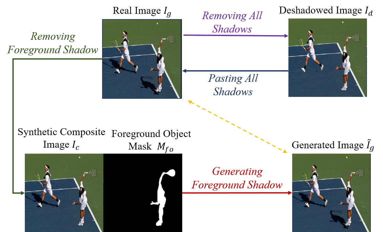
Figure 1: 1) The green arrows illustrate the process of acquiring paired data. We select a foreground object in the ground-truth target image $\mathbf{I}_{g}$, and replace its shadow area with the counterpart in deshadowed image $\mathbf{I}_{d}$ to synthesize a composite image $\mathbf{I}_{c}$. 2) The red arrow illustrates our shadow generation task. Given $\mathbf{I}_{c}$ and its foreground mask $\bm{M}_{fo}$, we aim to generate the target image $\tilde{\mathbf{I}}_{g}$ with foreground shadow.

Therefore, we tend to build our own real-world shadow generation dataset by synthesizing composite image from a ground-truth target image with object-shadow pairs. We build our dataset on the basis of Shadow-OBject Association (SOBA) dataset (Wang et al. 2020), which collects real-world images in complex scenes and provides annotated masks for object-shadow pairs. SOBA contains 3,623 pairs of shadow-object associations over 1000 images. Based on SOBA dataset, we remove all the shadows to construct our DEshadowed SOBA (DESOBA) dataset, which can be used for shadow generation task as well as other relevant vision applications. At the start, we tried to remove the shadows with the state-of-the-art deshadow methods (Zhang et al. 2020; Le and Samaras 2020; Cun, Pun, and Shi 2020). However, their performance is far from satisfactory due to complex scenes. Thus, with shadow images and shadow masks from SOBA datasets, we employ professional photo editors to manually remove the shadows in each image to obtain deshadowed images. We carefully check each deshadowed image to ensure that the background texture is maintained to the utmost, the transition over shadow boundary is smooth, and the original shadowed area cannot be identified. Although the deshadowed images may not be perfectly accurate, we show that the synthetic dataset is still useful for method comparison and real-world image composition. One example of ground-truth target image $\mathbf{I}_{g}$ and its deshadowed version $\mathbf{I}_{d}$ is shown in Figure 1. To obtain paired training data for shadow generation task, we choose a foreground object with associated shadow in the ground-truth target image $\mathbf{I}_{g}$ and replace its shadow area with the counterpart in the deshadowed image $\mathbf{I}_{d}$, yielding the synthetic composite image $\mathbf{I}_{c}$. In this way, pairs of synthetic composite image $\mathbf{I}_{c}$ and ground-truth target image $\mathbf{I}_{g}$ can be obtained.

With paired training data available, the shadow generation task can be defined as follows. Given an input composite image $\mathbf{I}_{c}$ and the foreground object mask $\mathbf{M}_{fo}$, the goal is to generate realistic shadow for the foreground object, resulting in the target image $\tilde{\mathbf{I}}_{g}$ which should be close to the ground-truth $\mathbf{I}_{g}$ (see Figure 1). For ease of description, we use foreground (resp., background) shadow to indicate the shadow of foreground (resp., background) object. Existing image-to-image translation methods (Isola et al. 2017; Zhu et al. 2017; Huang et al. 2018; Lin et al. 2018b) can be used for shadow generation, but they cannot achieve plausible shadows without considering illumination condition or shadow property. ShadowGAN (Zhang, Liang, and Wang 2019) was designed to generate shadows for virtual objects by combining a global discriminator and a local discriminator. ARShadowGAN (Liu et al. 2020) searched clues from background using attention mechanism to assist in shadow generation. However, the abovementioned methods did not model the thorough foreground-background interaction and did not leverage typical illumination model, which motivates us to propose a novel Shadow Generation in the Real-world Network (SGRNet) to generate shadows for the foreground objects in complex scenes.

As illustrated in Figure 3, SGRNet consists of a shadow mask prediction stage and a shadow filling stage. Such two-stage approach has not been explored in shadow generation task before. In the shadow mask prediction stage, provided with a synthetic composite image $\mathbf{I}_{c}$ and foreground object mask $\mathbf{M}_{fo}$, we design a foreground encoder to extract the required information of the foreground object and a background encoder to infer illumination information from background. To achieve thorough foreground and background information interaction, a cross-attention integration layer is employed to help generate shadow mask for the foreground object. The shadow filling stage is designed based on illumination model (Le and Samaras 2019), which first predicts the shadow property and then edits the shadow area. Besides, we design a conditional discriminator to distinguish real object-shadow-image triplets from fake triplets, which can push the generator to produce realistic foreground shadow. To verify the effectiveness of our proposed SGRNet, we conduct experiments on DESOBA dataset and real composite images. Our dataset and code are available at https://github.com/bcmi/Object-Shadow-Generation-Dataset-DESOBA.

Our main contributions are summarized as follows: 1) we contribute the first real-world shadow generation dataset DESOBA using a novel data acquisition approach; 2) we design a novel two-stage network SGRNet to generate shadow for the foreground object in composite image; 3) extensive experiments demonstrate the effectiveness of our way to construct dataset and the superiority of our network.

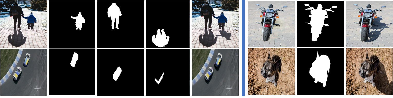
Figure 2: Some examples from our DESOBA dataset. BOS test image pairs with Background Object-Shadow (BOS) pairs are shown in the left subfigure, from left to right: synthetic composite image, foreground object mask, background object mask, background shadow mask, and ground-truth target image. BOS-free test image pairs are shown in the right subfigure, from left to right: synthetic composite image, foreground object mask, and ground-truth target image.

2 Related Work

2.1 Image Composition

Image composition (Niu et al. 2021) targets at pasting a foreground object on another background image to produce a composite image (Lin et al. 2018a; Wu et al. 2019; Zhan, Huang, and Lu 2019; Zhan et al. 2020b; Liu et al. 2020). Many issues would significantly degrade the quality of composite images, such as unreasonable location of foreground or inconsistent color/illumination between foreground and background. Previous works attempted to solve one or multiple issues. For example, image blending methods (Pérez, Gangnet, and Blake 2003; Wu et al. 2019; Zhang, Wen, and Shi 2020; Zhang et al. 2021) were developed to blend foreground and background seamlessly. Image harmonization methods (Tsai et al. 2017; Cun and Pun 2020; Cong et al. 2020, 2021) were proposed to address the color/illumination discrepancy between foreground and background. Some other approaches (Chen and Kae 2019; Weng et al. 2020; Zhan, Zhu, and Lu 2019) aimed to cope with the inconsistency of geometry, color, and boundary simultaneously. However, these methods did not consider the shadow effect of inserted foreground on background image, which is the focus of this paper.

2.2 Shadow Generation

Prior works on shadow generation can be divided into two groups: rendering based methods and image-to-image translation methods.

Shadow Generation via Rendering: This group of methods require explicit knowledge of illumination, reflectance, material properties, and scene geometry to generate shadow for inserted virtual object using rendering techniques. However, such knowledge is usually unavailable in the real-world applications. Some methods (Karsch et al. 2014; Kee, O’Brien, and Farid 2014; Liu, Xu, and Martin 2017) relied on user interaction to acquire illumination condition and scene geometry, which is time-consuming and labor-intensive. Without user interaction, some methods (Liao et al. 2019; Gardner et al. 2019; Zhang et al. 2019b; Arief, McCallum, and Hardeberg 2012) attempted to recover explicit illumination condition and scene geometry based on a single image, but this estimation task is quite tough and inaccurate estimation may lead to terrible results (Zhang, Liang, and Wang 2019).

Shadow Generation via Image-to-image Translation: This group of methods learn a mapping from the input image without foreground shadow to the output with foreground shadow, without requiring explicit knowledge of illumination, reflectance, material properties, and scene geometry. Most methods within this group have encoder-decoder network structures. For example, the shadow removal method Mask-ShadowGAN (Hu et al. 2019) could be adapted to shadow generation, but the cyclic generation procedure failed to generate shadows in complex scenes. ShadowGAN (Zhang, Liang, and Wang 2019) combined a global conditional discriminator and a local conditional discriminator to generate shadow for inserted 3D foreground objects without exploiting background illumination information. In (Zhan et al. 2020a), an adversarial image composition network was proposed for harmonization and shadow generation simultaneously, but it calls for extra indoor illumination dataset (Gardner et al. 2017; Cheng et al. 2018). ARShadowGAN (Liu et al. 2020) released Shadow-AR dataset and proposed an attention-guided network. Distinctive from the above works, our proposed SGRNet encourages thorough information interaction between foreground and background, and also leverages typical illumination model to guide network design.

3 Dataset Construction

We follow the training/test split in SOBA dataset (Wang et al. 2020). SOBA has $840$ training images with $2,999$ object-shadow pairs and $160$ test images with $624$ object-shadow pairs. We discard one complex training image whose shadow is hard to remove. Since most images in SOBA are outdoor images, we focus on outdoor illumination in this work. For each image in the training set, to obtain more training image pairs, we use a subset of foreground objects with associated shadows each time. Specifically, given a real image $\mathbf{I}_{g}$ with $n$ object-shadow pairs $\{(\mathbf{O}_{i},\mathbf{S}_{i})|_{i=1}^{n}\}$ and its deshadowed version $\mathbf{I}_{d}$ without shadows $\{\mathbf{S}_{i}|_{i=1}^{n}\}$, we randomly select a subset of foreground objects from $\mathbf{I}_{g}$ and replace their shadow areas with the counterparts in $\mathbf{I}_{d}$, leading to a synthetic composite image $\mathbf{I}_{c}$. In this way, based on the training set of SOBA, we can obtain abundant training image pairs of synthetic composite images and ground-truth target images. In Section 4, for ease of description, we treat a subset of foreground objects as one whole foreground object.

For the test set, we can get pairs of synthetic composite images and ground-truth target images in the same way. We focus on synthetic composite images with only one foreground object and ignore those with too small foreground shadow after the whole image is resized to $256\times 256$. Afterwards, we obtain $615$ test image pairs, which are divided into two groups according to whether they have background object-shadow pairs. Specifically, we refer to the test image pairs with Background Object-Shadow (BOS) pairs as BOS test image pairs, and the remaining ones as BOS-free test image pairs. Despite the absence of strong cues like background object-shadow pairs, the background in BOS-free images could also provide a set of illumination cues (e.g., shading, sky appearance variation) (Lalonde, Efros, and Narasimhan 2012; Zhang et al. 2019b). Some examples of BOS test image pairs and BOS-free test image pairs are shown in Figure 2.

4 Our Method

Given a synthetic composite image $\mathbf{I}_{c}$ without foreground shadow and the foreground object mask ${\bm{M}}_{fo}$, our proposed Shadow Generation in the Real-world Network (SGRNet) targets at generating $\tilde{\mathbf{I}}_{g}$ with foreground shadow. Our SGRNet consists of two stages: a shadow mask prediction stage and a shadow filling stage (see Figure 3). This two-stage approach enables the network to focus on one aspect (i.e., shadow shape or shadow intensity) in each stage, which has not been explored in previous shadow generation methods (Zhang, Liang, and Wang 2019; Zhan et al. 2020a; Liu et al. 2020). In the shadow mask prediction stage, a shadow mask generator $G_{S}$ with foreground branch and background branch is designed to generate shadow mask $\tilde{\bm{M}}_{fs}$. In the shadow filling stage, a shadow parameter predictor $E_{P}$ and a shadow matte generator $G_{M}$ are used to fill the shadow mask to produce the target image $\tilde{\mathbf{I}}_{g}$ with foreground shadow.

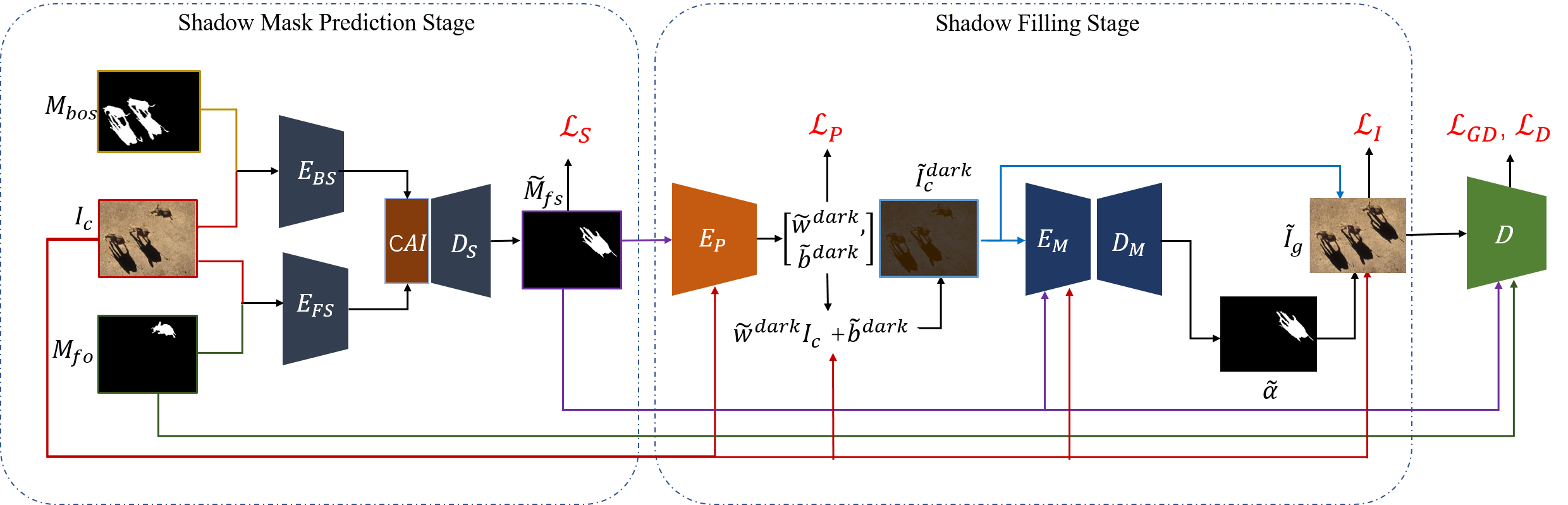
Figure 3: The framework of our SGRNet which consists of a shadow mask prediction stage and a shadow filling stage. In the shadow mask prediction stage, shadow mask $\tilde{\bm{M}}_{fs}$ is generated by the shadow mask generator composed of foreground encoder $E_{FS}$, background encoder $E_{BS}$, Cross-Attention Integration (CAI) layer, and decoder $D_{S}$. In the shadow filling stage, shadow parameters $\{\tilde{\bm{w}}^{dark},\tilde{\bm{b}}^{dark}\}$ are predicted by $E_{P}$ for producing darkened image $\tilde{\mathbf{I}}^{dark}_{c}$, and shadow matte predictor $G_{M}=\{E_{M},D_{M}\}$ generates shadow matte $\tilde{\bm{\alpha}}$. The final target image $\tilde{\mathbf{I}}_{g}$ is obtained by blending $\tilde{\mathbf{I}}^{dark}_{c}$ and $\mathbf{I}_{c}$ using $\tilde{\bm{\alpha}}$.

4.1 Shadow Mask Generator

The shadow mask generator $G_{S}$ aims to predict the binary shadow mask $\tilde{\bm{M}}_{fs}$ of the foreground object. We adopt U-Net (Ronneberger, Fischer, and Brox 2015) structure consisting of an encoder $E_{S}$ and a decoder $D_{S}$. To better extract foreground and background information, we split $E_{S}$ into a foreground encoder $E_{FS}$ and a background encoder $E_{BS}$. The foreground encoder $E_{FS}$ takes the concatenation of input composite image $\mathbf{I}_{c}$ and foreground object mask $\bm{M}_{fo}$ as input, producing the foreground feature map $\bm{X}_{f}=E_{FS}(\mathbf{I}_{c},\bm{M}_{fo})$. The background encoder $E_{BS}$ is expected to infer implicit illumination information from background. Considering that the background object-shadow pairs can provide strong illumination cues, we introduce background object-shadow mask $\bm{M}_{bos}$ enclosing all background object-shadow pairs. The background encoder $E_{BS}$ takes the concatenation of $\mathbf{I}_{c}$ and $\bm{M}_{bos}$ as input, producing the background feature map $\bm{X}_{b}=E_{BS}(\mathbf{I}_{c},\bm{M}_{bos})$.

The illumination information in different image regions may vary due to complicated scene geometry and light sources, which greatly increases the difficulty of shadow mask generation (Zhang, Liang, and Wang 2019). Thus, it is crucial to attend relevant illumination information to generate foreground shadow. Inspired by previous attention-based methods (Zhang et al. 2019a; Wang et al. 2018; Vaswani et al. 2017), we use a Cross-Attention Integration (CAI) layer to help foreground feature map $\bm{X}_{f}$ attend relevant illumination information from background feature map $\bm{X}_{b}$.

Firstly, $\bm{X}_{f}\in\mathbb{R}^{H\times W\times C}$ and $\bm{X}_{b}\in\mathbb{R}^{H\times W\times C}$ are projected to a common space by $f(\cdot)$ and $g(\cdot)$ respectively, where $f(\cdot)$ and $g(\cdot)$ are $1\times 1$ convolutional layer with spectral normalization (Miyato et al. 2018). For ease of calculation, we reshape $f(\bm{X}_{b})\in\mathbb{R}^{W\times H\times\frac{C}{8}}$ (resp., $g(\bm{X}_{f})\in\mathbb{R}^{W\times H\times\frac{C}{8}}$) into $\bar{f}(\bm{X}_{b})\in\mathbb{R}^{N\times\frac{C}{8}}$ (resp., $\bar{g}(\bm{X}_{f})\in\mathbb{R}^{N\times\frac{C}{8}}$), in which $N=W\times H$. Then, we can calculate the affinity map between $\bm{X}_{f}$ and $\bm{X}_{b}$:

$$\bm{A}=softmax\left(\bar{g}(\bm{X}_{f})\bar{f}(\bm{X}_{b})^{T}\right).$$ (1)

With obtained affinity map $\bm{A}$, we attend information from $\bm{X}_{b}$ and arrive at the attended feature map $\bm{X}_{b}^{\prime}$:

$$\bm{X}_{b}^{\prime}=v\left(\bm{A}\bar{h}(\bm{X}_{b})\right),$$ (2)

where $\bar{h}(\cdot)$ means $1\times 1$ convolutional layer followed by reshaping to $\mathbb{R}^{N\times\frac{C}{8}}$, similar to $\bar{f}(\cdot)$ and $\bar{g}(\cdot)$ in Eqn. 1. $v(\cdot)$ reshapes the feature map back to $\mathbb{R}^{W\times H\times\frac{C}{8}}$ and then performs $1\times 1$ convolution. Because the attended illumination information should be combined with the foreground information to generate foreground shadow mask, we concatenate $\bm{X}_{b}^{\prime}$ and $\bm{X}_{f}$, which is fed into the decoder $D_{S}$ to produce foreground shadow mask $\tilde{\bm{M}}_{fs}$:

$$\tilde{\bm{M}}_{fs}=D_{S}([\bm{X}_{b}^{\prime},\bm{X}_{f}]),$$ (3)

which is enforced to be close to the ground-truth foreground shadow mask $\bm{M}_{fs}$ by

$$\mathcal{L}_{S}=||\bm{M}_{fs}-\tilde{\bm{M}}_{fs}||_{2}^{2}.$$ (4)

Although cross attention is not a new idea, this is the first time to achieve foreground-background interaction via cross-attention in shadow generation task.

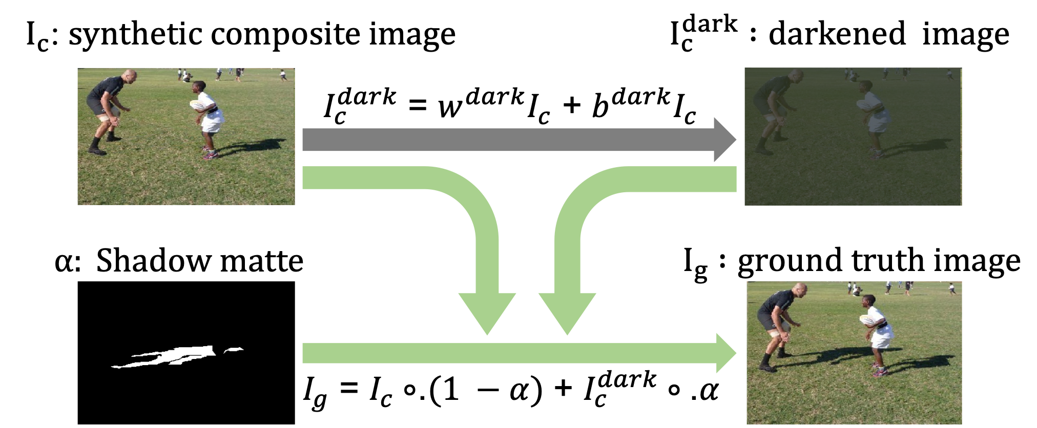
Figure 4: Shadow generation via image composition. The ground-truth target image $\mathbf{I}_{g}$ with foreground shadow can be expressed as the combination of synthetic composite image $\mathbf{I}_{c}$ and darkened image $\mathbf{I}_{c}^{dark}$ with shadow matte $\alpha$.

4.2 Shadow Area Filling

We design our shadow filling stage based on the illumination model used in  (Shor and Lischinski 2008; Le and Samaras 2019). According to (Shor and Lischinski 2008; Le and Samaras 2019), the value of a shadow-free pixel $I^{lit}(k,i)$ can be linearly transformed from its shadowed value $I^{dark}(k,i)$:

$$I^{lit}(k,i)=w^{lit}(k)I^{dark}(k,i)+b^{lit}(k),$$ (5)

in which $I(k,i)$ represents the value of the pixel $i$ in color channel $k$ ($k\in R,G,B$). $w^{lit}(k)$ and $b^{lit}(k)$ are constant across all pixels in the umbra area of the shadow. Inversely, the value of a shadowed pixel $I^{dark}(k,i)$ can be linearly transformed from its shadow-free value $I^{lit}(k,i)$:

$$I^{dark}(k,i)=w^{dark}(k)I^{lit}(k,i)+b^{dark}(k).$$ (6)

To accurately locate the foreground shadow area, we tend to learn a soft shadow matte $\bm{\alpha}$. The value of $\bm{\alpha}$ is 0 in the non-shadow area, 1 in the umbra of shadow area, and varying gradually in the penumbra of shadow area. Then, the target image with foreground shadow can be obtained using the following composition system (see Figure 4):

$$\mathbf{I}_{g}=\mathbf{I}_{c}\circ(\mathbf{1}-{\bm{\alpha}})+\mathbf{I}_{c}^{dark}\circ{\bm{\alpha}},$$ (7)

$$\mathbf{I}_{c}^{dark}(k)=w^{dark}(k)\mathbf{I}_{c}(k)+b^{dark}(k),$$ (8)

in which $\circ$ means element-wise multiplication, $\mathbf{I}(k)$ represents image $\mathbf{I}$ in color channel $k$, $\mathbf{I}_{c}^{dark}(k)$ is the darkened version of $\mathbf{I}_{c}(k)$ through Eqn. 8. $\mathbf{w}^{dark}=[w^{dark}(R),w^{dark}(G),w^{dark}(B)]$ and similarly defined $\mathbf{b}^{dark}$ are called shadow parameters. Given paired images $\{\mathbf{I}_{c},\mathbf{I}_{g}\}$, the ground-truth shadow parameter $\{\mathbf{w}^{dark},\mathbf{b}^{dark}\}$ for the foreground shadow can be easily calculated by using linear regression (Shor and Lischinski 2008). Specifically, we need to calculate the optimal regression coefficients $\{\mathbf{w}^{dark},\mathbf{b}^{dark}\}$ which regress pixel values $\mathbf{I}_{c}(k,i)$ to $\mathbf{I}_{g}(k,i)$ in the foreground shadow area. The ground-truth shadow parameters of training images can be precomputed before training, but the ground-truth shadow parameters of test images are unavailable in the testing stage. Thus, we learn a shadow parameter predictor $E_{P}$ to estimate $\{\mathbf{w}^{dark},\mathbf{b}^{dark}\}$.

Our $E_{P}$ is implemented as an encoder, which takes the concatenation of composite image ${\mathbf{I}}_{c}$ and predicted shadow mask $\tilde{\bm{M}}_{fs}$ as input to predict the shadow parameters $\{\tilde{\bm{w}}^{dark},\tilde{\bm{b}}^{dark}\}$:

$$\{\tilde{\bm{w}}^{dark},\tilde{\bm{b}}^{dark}\}=E_{P}({\mathbf{I}}_{c},\tilde{\bm{M}}_{fs}).$$ (9)

$\{\tilde{\bm{w}}^{dark},\tilde{\bm{b}}^{dark}\}$ are supervised with ground-truth shadow parameters $\{\bm{w}^{dark},\bm{b}^{dark}\}$ by regression loss:

$$\mathcal{L}_{P}=||\bm{w}^{dark}-\tilde{\bm{w}}^{dark}||_{2}^{2}+||\bm{b}^{dark}-\tilde{\bm{b}}^{dark}||_{2}^{2}.$$ (10)

After estimating $\{\tilde{\bm{w}}^{dark},\tilde{\bm{b}}^{dark}\}$, we can get the darkened image $\tilde{\mathbf{I}}_{c}^{dark}(k)=\tilde{w}^{dark}(k)\mathbf{I}_{c}(k)+\tilde{b}^{dark}(k)$ via Eqn. 8. Then, to obtain the final target image, we need to learn a shadow matte $\bm{\alpha}$ for image composition as in Eqn. 7. Our shadow matte generator $G_{M}$ is based on U-Net (Ronneberger, Fischer, and Brox 2015) with encoder $E_{M}$ and decoder $D_{M}$. $G_{M}$ concatenates composite image $\mathbf{I}_{c}$, darkened image $\tilde{\mathbf{I}}_{c}^{dark}$, and predicted shadow mask $\tilde{\bm{M}}_{fs}$ as input, producing the shadow matte $\tilde{\bm{\alpha}}$:

$$\tilde{\bm{\alpha}}=G_{M}(\mathbf{I}_{c},\tilde{\mathbf{I}}_{c}^{dark},\tilde{\bm{M}}_{fs}).$$ (11)

Finally, based on $\tilde{\mathbf{I}}_{c}^{dark}$, $\mathbf{I}_{c}$, and $\tilde{\bm{\alpha}}$, the target image with foreground shadow can be composed by

$$\tilde{\mathbf{I}}_{g}=\mathbf{I}_{c}\circ(\mathbf{1}-\tilde{\bm{\alpha}})+\tilde{\mathbf{I}}_{c}^{dark}\circ\tilde{\bm{\alpha}}.$$ (12)

The generated target image is supervised by the ground-truth target image with a reconstruction loss:

$$\mathcal{L}_{I}=||\mathbf{I}_{g}-\tilde{\mathbf{I}}_{g}||_{2}^{2}.$$ (13)

To the best of our knowledge, we are the first to generate shadow by blending original image and darkened image.

4.3 Conditional Discriminator

To ensure that the generated shadow mask $\tilde{\bm{M}}_{fs}$ and the generated target image $\tilde{\mathbf{I}}_{g}$ are close to real shadow mask $\bm{M}_{fs}$ and real target image $\mathbf{I}_{g}$ respectively, we design a conditional discriminator $D$ to bridge the gap between the generated triplet $\{\tilde{\bm{M}}_{fs},\tilde{\mathbf{I}}_{g},\bm{M}_{fo}\}$ and the real triplet $\{\bm{{M}}_{fs},\mathbf{I}_{g},\bm{M}_{fo}\}$. The architecture of our conditional discriminator is similar to Patch-GAN (Isola et al. 2017), which takes the concatenation of triplet as input. We adopt the hinge adversarial loss (Miyato and Koyama 2018) as follows,

$$\mathcal{L}_{D}=\mathbb{E}_{\tilde{\bm{M}}_{fs},\tilde{\mathbf{I}}_{g},\bm{M}_{fo}}[\max(0,1+\mathrm{D}(\tilde{\bm{M}}_{fs},\tilde{\mathbf{I}}_{g},\bm{M}_{fo}))]+$$

$$\quad\quad\mathbb{E}_{\bm{{M}}_{fs},\mathbf{I}_{g},\bm{M}_{fo}}[\max(0,1-\mathrm{D}(\bm{{M}}_{fs},\mathbf{I}_{g},\bm{M}_{fo})],$$

$$\mathcal{L}_{GD}=-\mathbb{E}_{\tilde{\bm{M}}_{fs},\tilde{\mathbf{I}}_{g},\bm{M}_{fo}}[\mathrm{D}(\tilde{\bm{M}}_{fs},\tilde{\mathbf{I}}_{g},\bm{M}_{fo})].$$ (14)

Method	BOS Test Images				BOS-free Test Images
	GRMSE $\downarrow$	LRMSE $\downarrow$	GSSIM $\uparrow$	LSSIM $\uparrow$	GRMSE $\downarrow$	LRMSE $\downarrow$	GSSIM $\uparrow$	LSSIM $\uparrow$
Pix2Pix	7.659	75.346	0.926	0.249	18.875	81.444	0.858	0.110
Pix2Pix-Res	5.961	76.046	0.971	0.253	18.365	81.966	0.901	0.107
ShadowGAN	5.985	78.412	0.984	0.240	19.306	87.017	0.918	0.078
Mask-ShadowGAN	8.287	79.212	0.952	0.245	19.475	83.457	0.891	0.109
ARShadowGAN	6.481	75.099	0.983	0.251	18.723	81.272	0.917	0.109
Ours	4.754	61.763	0.988	0.380	15.128	61.439	0.928	0.183

Table 1: Results of quantitative comparison on our DESOBA dataset.

4.4 Optimization

The overall optimization function can be written as

$$\mathcal{L}=\lambda_{S}\mathcal{L}_{S}+\lambda_{I}\mathcal{L}_{I}+\lambda_{P}\mathcal{L}_{P}+\lambda_{GD}\mathcal{L}_{GD}+\mathcal{L}_{D},$$ (15)

where $\lambda_{S}$, $\lambda_{I}$, $\lambda_{P}$, and $\lambda_{GD}$ are trade-off parameters.

The parameters of $\{E_{S},CAI,D_{S},E_{P},E_{M},D_{M}\}$ are denoted as $\theta_{G}$, while the parameters of $D$ are denoted as $\theta_{D}$. Following adversarial learning framework (Gulrajani et al. 2017), we use related loss terms to optimize $\theta_{G}$ and $\theta_{D}$ alternatingly. In detail, $\theta_{D}$ is optimized by minimizing $\mathcal{L}_{D}$. Then, $\theta_{G}$ is optimized by minimizing $\lambda_{S}\mathcal{L}_{S}+\lambda_{I}\mathcal{L}_{I}+\lambda_{P}\mathcal{L}_{P}+\lambda_{GD}\mathcal{L}_{GD}$.

5 Experiments

5.1 Experimental Setup

Datasets We conduct experiments on our constructed DESOBA dataset and real composite images. On DESOBA dataset, we perform both quantitative and qualitative evaluation based on $615$ test image pairs with one foreground, which are divided into $581$ BOS test image pairs and $34$ BOS-free test image pairs. We also show the qualitative results of test images with two foregrounds in Supplementary. The experiments on real composite images will be described in Supplementary due to space limitation.

Implementation After a few trials, we set $\lambda_{S}=\lambda_{I}=10$, $\lambda_{P}=1$, and $\lambda_{GD}=0.1$ by observing the generated images during training. We use Pytorch $1.3.0$ to implement our model, which is distributed on RTX 2080 Ti GPU. All images in our used datasets are resized to $256\times 256$ for training and testing. We use adam optimizer with the learning rate initialized as $0.0002$ and $\beta$ set to $(0.5,0.99)$. The batch size is $1$ and our model is trained for $50$ epochs.

Baselines Following (Liu et al. 2020), we select Pix2Pix (Isola et al. 2017), Pix2Pix-Res, ShadowGAN (Zhang, Liang, and Wang 2019), ARShadowGAN (Liu et al. 2020), and Mask-ShadowGAN (Hu et al. 2019) as baselines. Pix2Pix (Isola et al. 2017) is a popular image-to-image translation method, which takes composite image as input and outputs target image. Pix2Pix-Res has the same architecture as Pix2Pix except producing a residual image, which is added to the input image to generate the target image. ShadowGAN (Zhang, Liang, and Wang 2019) and ARShadowGAN (Liu et al. 2020) are two closely related methods, which can be directly applied to our task. Mask-ShadowGAN (Hu et al. 2019) originally performs both mask-free shadow removal and mask-guided shadow generation. We adapt it to our task by exchanging two generators to perform mask-guided shadow removal and mask-free shadow generation, in which the mask-free shadow generator can be used in our task.

Evaluation Metrics Following (Liu et al. 2020), we adopt Root Mean Square Error (RMSE) and Structural SIMilarity index (SSIM). RMSE and SSIM are calculated based on the ground-truth target image and the generated target image. Global RMSE (GRMSE) and Global SSIM (GSSIM) are calculated over the whole image, while Local RMSE (LRMSE) and Local SSIM (LSSIM) are calculated over the ground-truth foreground shadow area.

5.2 Evaluation on Our DESOBA Dataset

On DESOBA dataset, BOS test set and BOS-free test set are evaluated separately and the comparison results are summarized in Table 1. We can observe that our SGRNet achieves the lowest GRMSE, LRMSE and the highest GSSIM, LSSIM, which demonstrates that our method could generate more realistic and compatible shadows for foreground objects compared with baselines. The difference between the results on BOS test set and BOS-free test set is partially caused by the size of foreground shadow, because BOS-free test images usually have larger foreground shadows than BOS test images as shown in Figure 2. We will provide more in-depth comparison by controlling the foreground shadow size in Supplementary.

For qualitative comparison, we show some example images generated by our SGRNet and other baselines on BOS and BOS-free test images in Figure 5. We can see that our SGRNet can generally generate foreground shadows with reasonable shapes and shadow directions compatible with the object-shadow pairs in background. In contrast, other baselines produce foreground shadows with implausible shapes, or even fail to produce any shadow. Our method can also generate reasonable shadows for BOS-free test images, because the background in BOS-free images could also provide a set of illumination cues (e.g., shading, sky appearance variation) (Lalonde, Efros, and Narasimhan 2012; Zhang et al. 2019b) as discussed in Section 3. More visualization results including the intermediate results (e.g., generated foreground shadow mask, generated darkened image) can be found in Supplementary.

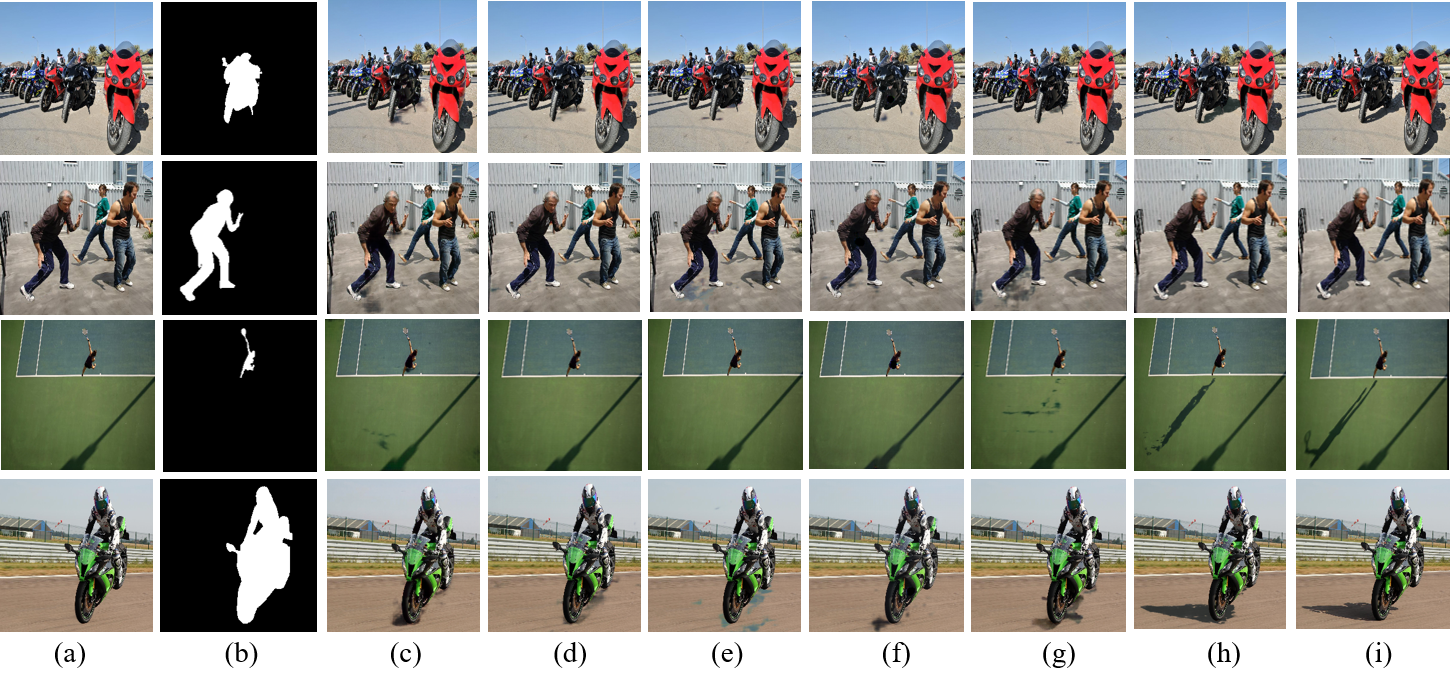
Figure 5: Visualization comparison on our DESOBA dataset. From left to right are input composite image (a), foreground object mask (b), results of Pix2Pix (c), Pix2Pix-Res (d), ShadowGAN (e), Mask-ShadowGAN (f), ARShadowGAN (g), our SGRNet (h), ground-truth (i). The results on BOS (resp., BOS-free) test images are shown in row 1-2 (resp., 3-4).

Method	GRMSE $\downarrow$	LRMSE $\downarrow$	GSSIM $\uparrow$	LSSIM$\uparrow$
w/o $E_{BS}$	5.549	68.876	0.985	0.317
w/o CAI	5.106	68.031	0.986	0.320
w/o $\mathbf{M}_{bos}$	4.931	63.141	0.986	0.358
w/o Fill	5.328	67.789	0.941	0.255
w/o $\mathcal{L}_{P}$	4.929	65.054	0.986	0.352
Naive D	5.059	65.238	0.987	0.355
w/o $\mathcal{L}_{GD}$	5.453	67.056	0.986	0.348
Ours	4.754	61.763	0.988	0.380

Table 2: Ablation studies of loss terms and alternative network designs on BOS test images from DESOBA dataset.

5.3 Ablation Studies

We analyze the impact of loss terms and alternative network designs of our SGRNet on BOS test images from DESOBA dataset. Quantitative results are reported in Table 2.

Shadow mask prediction stage: To investigate the necessity of background encoder, we remove the background encoder $E_{BS}$, which is referred to as “w/o $E_{BS}$” in Table 2. To verify the effectiveness of Cross-Attention Integration (CAI) layer, we remove CAI layer and directly concatenate $[\bm{X}_{f},\bm{X}_{b}]$, which is referred to as “w/o CAI”. The performance of “w/o CAI” is better than “w/o $E_{BS}$”, which shows the advantage of extracting foreground and background information separately. The performance of “w/o CAI” is worse than our full method, which shows the benefit of encouraging thorough information interaction between foreground and background. To study the importance of background object-shadow mask, we set the value of $\mathbf{M}_{bos}$ as zero, which is referred to as “w/o $\mathbf{M}_{bos}$”. The performance is better than “w/o $E_{BS}$” and “w/o CAI”, which can be explained as follows. CAI layer can help foreground encoder exploit illumination information from background, even without explicit background object-shadow mask. The comparison between “w/o $\mathbf{M}_{bos}$” and full method proves that background object-shadow mask can indeed provide useful shadow cues as guidance.

Shadow filling stage: To corroborate the superiority of image composition system in Section 4, we replace our $E_{P}$ and $\{E_{M},D_{M}\}$ with a U-Net (Ronneberger, Fischer, and Brox 2015) model which takes $\tilde{\mathbf{M}}_{fs}$ and $\mathbf{I}_{c}$ as input to generate the final target image directly, which is referred to as “w/o Fill” in Table 2. The result is worse than full method, which demonstrates the advantage of composition system. We also remove the supervision for shadow parameters by setting $\mathcal{L}_{P}=0$, which is referred to as “w/o $\mathcal{L}_{P}$”. We find that the performance is better than “w/o Fill” but worse than full method, which demonstrates the necessity of supervision from ground-truth shadow parameters.

Adversarial learning: We remove conditional information $\{\bm{M}_{fo},\bm{M}_{fs}\}$ (resp., $\{\bm{M}_{fo},\tilde{\bm{M}}_{fs}\}$), and only feed $\mathbf{I}_{g}$ (resp., $\tilde{\mathbf{I}}_{g}$) into the discriminator $D$, which is named as “Naive D” in Table 2. It can be seen that conditional discriminator can enhance the quality of generated images. To further investigate the effect of adversarial learning, we remove the adversarial loss $\mathcal{L}_{GD}$ from Eqn. 15 and report the result as “w/o $\mathcal{L}_{GD}$”. The result is worse than “Naive D”, which indicates that adversarial learning can help generate more realistic foreground shadows.

We visualize some examples produced by different ablated methods and conduct ablation studies on BOS-free test images in Supplementary.

5.4 Evaluation on Real Composite Images

To obtain real composite images, we select test images from DESOBA as background images, and paste foreground objects also from test images at reasonable locations on the background images. In this way, we create $100$ real composite images without foreground shadows for evaluation. Because real composite images do not have ground-truth target images, it is impossible to perform quantitative evaluation. Therefore, we conduct user study on the $100$ composite images for subjective evaluation. The visualization results and user study are left to Supplementary.

6 Conclusion

In this work, we have contributed a real-world shadow generation dataset DESOBA. We have also proposed SGRNet, a novel shadow generation method, which can predict shadow mask by inferring illumination information from background and estimate shadow parameters based on illumination model. The promising results on our constructed dataset and real composite images have demonstrated the effectiveness of our method.

References

- Arief, McCallum, and Hardeberg (2012) Arief, I.; McCallum, S.; and Hardeberg, J. Y. 2012. Realtime estimation of illumination direction for augmented reality on mobile devices. In CIC.
- Azadi et al. (2019) Azadi, S.; Pathak, D.; Ebrahimi, S.; and Darrell, T. 2019. Compositional GAN (Extended Abstract): Learning Image-Conditional Binary Composition. In ICLR 2019 Workshop.
- Azadi et al. (2020) Azadi, S.; Pathak, D.; Ebrahimi, S.; and Darrell, T. 2020. Compositional gan: Learning image-conditional binary composition. IJCV, 128(10): 2570–2585.
- Chen and Kae (2019) Chen, B.-C.; and Kae, A. 2019. Toward realistic image compositing with adversarial learning. In CVPR.
- Cheng et al. (2018) Cheng, D.; Shi, J.; Chen, Y.; Deng, X.; and Zhang, X. 2018. Learning Scene Illumination by Pairwise Photos from Rear and Front Mobile Cameras. Comput. Graph. Forum, 37(7): 213–221.
- Cong et al. (2021) Cong, W.; Niu, L.; Zhang, J.; Liang, J.; and Zhang, L. 2021. Bargainnet: Background-Guided Domain Translation for Image Harmonization. In ICME.
- Cong et al. (2020) Cong, W.; Zhang, J.; Niu, L.; Liu, L.; Ling, Z.; Li, W.; and Zhang, L. 2020. Dovenet: Deep image harmonization via domain verification. In CVPR.
- Cun and Pun (2020) Cun, X.; and Pun, C. 2020. Improving the Harmony of the Composite Image by Spatial-Separated Attention Module. TIP.
- Cun, Pun, and Shi (2020) Cun, X.; Pun, C.-M.; and Shi, C. 2020. Towards ghost-free shadow removal via dual hierarchical aggregation network and shadow matting GAN. In AAAI.
- Gardner et al. (2019) Gardner, M.-A.; Hold-Geoffroy, Y.; Sunkavalli, K.; Gagné, C.; and Lalonde, J.-F. 2019. Deep parametric indoor lighting estimation. In ICCV.
- Gardner et al. (2017) Gardner, M.-A.; Sunkavalli, K.; Yumer, E.; Shen, X.; Gambaretto, E.; Gagné, C.; and Lalonde, J.-F. 2017. Learning to predict indoor illumination from a single image. ACM Transactions on Graphics (TOG), 36(6): 1–14.
- Gulrajani et al. (2017) Gulrajani, I.; Ahmed, F.; Arjovsky, M.; Dumoulin, V.; and Courville, A. C. 2017. Improved training of wasserstein GANs. In NeurIPS.
- Hu et al. (2019) Hu, X.; Jiang, Y.; Fu, C.-W.; and Heng, P.-A. 2019. Mask-ShadowGAN: Learning to remove shadows from unpaired data. In ICCV.
- Huang et al. (2018) Huang, X.; Liu, M.-Y.; Belongie, S.; and Kautz, J. 2018. Multimodal unsupervised image-to-image translation. In ECCV.
- Isola et al. (2017) Isola, P.; Zhu, J.-Y.; Zhou, T.; and Efros, A. A. 2017. Image-to-Image Translation with Conditional Adversarial Networks. In CVPR.
- Karsch et al. (2014) Karsch, K.; Sunkavalli, K.; Hadap, S.; Carr, N.; Jin, H.; Fonte, R.; Sittig, M.; and Forsyth, D. 2014. Automatic scene inference for 3d object compositing. ACM Transactions on Graphics (TOG), 33(3): 1–15.
- Kee, O’Brien, and Farid (2014) Kee, E.; O’Brien, J. F.; and Farid, H. S. 2014. Exposing Photo Manipulation from Shading and Shadows. ACM Transactions on Graphics (TOG).
- Lalonde, Efros, and Narasimhan (2012) Lalonde, J.-F.; Efros, A. A.; and Narasimhan, S. G. 2012. Estimating the natural illumination conditions from a single outdoor image. IJCV, 98(2): 123–145.
- Le and Samaras (2019) Le, H.; and Samaras, D. 2019. Shadow removal via shadow image decomposition. In ICCV.
- Le and Samaras (2020) Le, H.; and Samaras, D. 2020. From Shadow Segmentation to Shadow Removal. In ECCV.
- Liao et al. (2019) Liao, B.; Zhu, Y.; Liang, C.; Luo, F.; and Xiao, C. 2019. Illumination animating and editing in a single picture using scene structure estimation. Computers & Graphics, 82: 53–64.
- Lin et al. (2018a) Lin, C.-H.; Yumer, E.; Wang, O.; Shechtman, E.; and Lucey, S. 2018a. St-gan: Spatial transformer generative adversarial networks for image compositing. In CVPR.
- Lin et al. (2018b) Lin, J.; Xia, Y.; Qin, T.; Chen, Z.; and Liu, T.-Y. 2018b. Conditional image-to-image translation. In CVPR.
- Liu, Xu, and Martin (2017) Liu, B.; Xu, K.; and Martin, R. R. 2017. Static scene illumination estimation from videos with applications. Journal of Computer Science and Technology, 32(3): 430–442.
- Liu et al. (2020) Liu, D.; Long, C.; Zhang, H.; Yu, H.; Dong, X.; and Xiao, C. 2020. Arshadowgan: Shadow generative adversarial network for augmented reality in single light scenes. In CVPR.
- Miyato et al. (2018) Miyato, T.; Kataoka, T.; Koyama, M.; and Yoshida, Y. 2018. Spectral Normalization for Generative Adversarial Networks. In ICLR.
- Miyato and Koyama (2018) Miyato, T.; and Koyama, M. 2018. cGANs with Projection Discriminator. In ICLR.
- Niu et al. (2021) Niu, L.; Cong, W.; Liu, L.; Hong, Y.; Zhang, B.; Liang, J.; and Zhang, L. 2021. Making Images Real Again: A Comprehensive Survey on Deep Image Composition. arXiv preprint arXiv:2106.14490.
- Pérez, Gangnet, and Blake (2003) Pérez, P.; Gangnet, M.; and Blake, A. 2003. Poisson image editing. In ACM SIGGRAPH 2003 Papers, 313–318. ACM.
- Ronneberger, Fischer, and Brox (2015) Ronneberger, O.; Fischer, P.; and Brox, T. 2015. U-net: Convolutional networks for biomedical image segmentation. In MICCAI.
- Shor and Lischinski (2008) Shor, Y.; and Lischinski, D. 2008. The shadow meets the mask: Pyramid-based shadow removal. In Computer Graphics Forum, 577–586.
- Tsai et al. (2017) Tsai, Y.; Shen, X.; Lin, Z.; Sunkavalli, K.; Lu, X.; and Yang, M. 2017. Deep Image Harmonization. In CVPR.
- van Steenkiste et al. (2020) van Steenkiste, S.; Kurach, K.; Schmidhuber, J.; and Gelly, S. 2020. Investigating object compositionality in generative adversarial networks. Neural Networks, 130: 309–325.
- Vaswani et al. (2017) Vaswani, A.; Shazeer, N.; Parmar, N.; Uszkoreit, J.; Jones, L.; Gomez, A. N.; Kaiser, L.; and Polosukhin, I. 2017. Attention is all you need. NeurIPS.
- Wang et al. (2020) Wang, T.; Hu, X.; Wang, Q.; Heng, P.-A.; and Fu, C.-W. 2020. Instance shadow detection. In CVPR.
- Wang et al. (2018) Wang, X.; Girshick, R.; Gupta, A.; and He, K. 2018. Non-local neural networks. In CVPR.
- Weng et al. (2020) Weng, S.; Li, W.; Li, D.; Jin, H.; and Shi, B. 2020. Misc: Multi-condition injection and spatially-adaptive compositing for conditional person image synthesis. In CVPR.
- Wu et al. (2019) Wu, H.; Zheng, S.; Zhang, J.; and Huang, K. 2019. Gp-gan: Towards realistic high-resolution image blending. In ACM MM.
- Zhan, Huang, and Lu (2019) Zhan, F.; Huang, J.; and Lu, S. 2019. Adaptive composition gan towards realistic image synthesis. arXiv preprint arXiv:1905.04693.
- Zhan et al. (2020a) Zhan, F.; Lu, S.; Zhang, C.; Ma, F.; and Xie, X. 2020a. Adversarial Image Composition with Auxiliary Illumination. In ACCV.
- Zhan et al. (2020b) Zhan, F.; Lu, S.; Zhang, C.; Ma, F.; and Xie, X. 2020b. Towards realistic 3d embedding via view alignment. arXiv preprint arXiv:2007.07066.
- Zhan, Zhu, and Lu (2019) Zhan, F.; Zhu, H.; and Lu, S. 2019. Spatial fusion gan for image synthesis. In CVPR.
- Zhang et al. (2019a) Zhang, H.; Goodfellow, I.; Metaxas, D.; and Odena, A. 2019a. Self-Attention generative adversarial networks. In ICML.
- Zhang et al. (2021) Zhang, H.; Zhang, J.; Perazzi, F.; Lin, Z.; and Patel, V. M. 2021. Deep Image Compositing. In WACV.
- Zhang et al. (2019b) Zhang, J.; Sunkavalli, K.; Hold-Geoffroy, Y.; Hadap, S.; Eisenman, J.; and Lalonde, J.-F. 2019b. All-weather deep outdoor lighting estimation. In CVPR.
- Zhang et al. (2020) Zhang, L.; Long, C.; Zhang, X.; and Xiao, C. 2020. Ris-gan: Explore residual and illumination with generative adversarial networks for shadow removal. In AAAI.
- Zhang, Wen, and Shi (2020) Zhang, L.; Wen, T.; and Shi, J. 2020. Deep image blending. In WACV.
- Zhang, Liang, and Wang (2019) Zhang, S.; Liang, R.; and Wang, M. 2019. Shadowgan: Shadow synthesis for virtual objects with conditional adversarial networks. Computational Visual Media, 5(1): 105–115.
- Zhu et al. (2017) Zhu, J.-Y.; Park, T.; Isola, P.; and Efros, A. A. 2017. Unpaired image-to-image translation using cycle-consistent adversarial networks. In ICCV.