BADet: Boundary-Aware 3D Object Detection from Point Clouds

Abstract

Currently, existing state-of-the-art 3D object detectors are in two-stage paradigm. These methods typically comprise two steps: 1) Utilize a region proposal network to propose a handful of high-quality proposals in a bottom-up fashion. 2) Resize and pool the semantic features from the proposed regions to summarize RoI-wise representations for further refinement. Note that these RoI-wise representations in step 2) are considered individually as uncorrelated entries when fed to following detection headers. Nevertheless, we observe these proposals generated by step 1) offset from ground truth somehow, emerging in local neighborhood densely with an underlying probability. Challenges arise in the case where a proposal largely forsakes its boundary information due to coordinate offset while existing networks lack corresponding information compensation mechanism. In this paper, we propose BADet for 3D object detection from point clouds. Specifically, instead of refining each proposal independently as previous works do, we represent each proposal as a node for graph construction within a given cut-off threshold, associating proposals in the form of local neighborhood graph, with boundary correlations of an object being explicitly exploited. Besides, we devise a lightweight Region Feature Aggregation Module to fully exploit voxel-wise, pixel-wise, and point-wise features with expanding receptive fields for more informative RoI-wise representations. We validate BADet both on widely used KITTI Dataset and highly challenging nuScenes Dataset. As of Apr. 17th, 2021, our BADet achieves on par performance on KITTI 3D detection leaderboard and ranks $1^{st}$ on $Moderate$ difficulty of $Car$ category on KITTI BEV detection leaderboard. The source code is available at https://github.com/rui-qian/BADet.

© 2022 Elsevier Ltd. All rights reserved.

© 2022 Elsevier Ltd. All rights reserved.

1 INTRODUCTION

Scene understanding has been a long-term interest of pattern recognition [1, 2, 3, 4]. 3D object detection, as a key step towards scene understanding in the real world, is to estimate 3D bounding boxes of real objects from sensory data. Point clouds, which effectively capture informative geometric attributes such as 3D positions, orientations and occupied volumes, are increasingly prevalent sensor data, in particular for 3D object detection in driving scenes [5, 6, 7]. Despite existing efforts [8, 9, 10], 3D object detection has still trailed 2D counterparts thus far [11, 12, 13]. This paper is targeted at detecting 3D objects from point clouds.

Depending on how feature representation learning is performed on point clouds, we categorize the state-of-the-art into the following three groups, i.e. voxel-based, point-based, and point-voxel-based methods. Voxel-based methods [14, 15, 16] generally rasterize irregularly distributed point clouds into volumetric grids to extract features from regular domains. Point-based methods [17, 18, 19] directly consume raw point clouds to abstract features from irregular domains. Very recently, a large body of investigations have been looking into fusing the best of two worlds together for synergies. Point-voxel-based methods [6, 5, 20] are proposed as a joint treatment for learning more informative representations from both regular and irregular domains.

Given features extracted from the point clouds, recent high-performance 3D object detectors share a two-step working pipeline. First, a region proposal network (RPN) [12] is utilized to produce a number of high-quality region-of-interest (RoI) proposals in a bottom-up fashion. RoI proposals w.r.t. a specific object tend to densely appear surrounding the object, as visualized in red bounding boxes in Fig. 1. Second, RoI pooling is performed separately on each of the bounding boxes to obtain RoI-wise representations for further refinement. It is worth pointing out that in the previous works, these RoI-wise representations, despite their apparent spatial correlations, are treated as uncorrelated entries and thus fed independently to a subsequent detection header. As illustrated in Fig. 1, proposals in (b) are exactly what we anticipate. In contrast, proposals in (a), (c) and (d) all deviate from their ground truth to some extent, either in terms of their azimuth or by their positions. Importantly, such deviation becomes even more severe at long ranges where point clouds are sparse by nature. Challenges arise in the case where a proposal largely forsakes its boundary information due to coordinate offset while existing networks lack corresponding information compensation mechanism. As a result, once the deviation occurs, an RoI proposal alone is insufficient to capture the boundary information of the underlying object it belongs to. On the basis of above discussion and analysis, an important research question arises as how to exploit the spatial correlations among the RoI proposals so that each of them will possess the whole receptive field of the associated object?

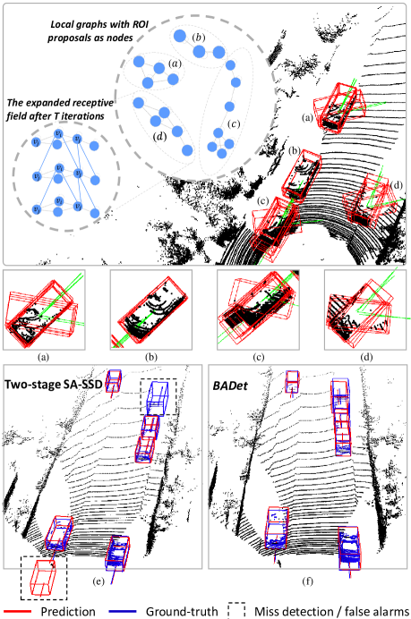
Figure 1: Two-stage SA-SSD [5] vs. BADet. Ideal proposals as shown in (b) are relatively rare. Typical proposals deviate from their ground truth, as shown in (a), (c) and (d). While proposal refinement is indispensible, the prior art treats the proposals independently without explicitly taking their spatial correlations into account. By contrast, we propose to model such correlations by graph neural networks (GNN), see the top part of the figure. Compared to 3D object detection results of the baseline (e) , our proposed BADet model has less miss detection and fewer false alarms (f). Note that (e) and (f) show different viewpoints of the same point clouds. Two-stage SA-SSD is implemented by directly adding a BEV detect head on the top of the 2D backbone network in the SA-SSD for fair comparison.

Bearing this in mind, we answer the above question by proposing BADet, a novel Boundary-Aware 3D object Detection network. In particular, the object boundary-aware property of our model is achieved by graph neural networks (GNN) [19] based modeling. Fig. 1 shows graph representations of the proposals within a specific neighborhood. Different from the existing works, e.g. STD [20], PV-RCNN [6] and PointRCNN [17], which refine each proposal independently, we consider each proposal in a given neighborhood as a node in a local neighborhood graph. As such, their spatial correlations are naturally modeled by GNN feature representation learning. With messages exchanged between the nodes in an iterative manner, the receptive field of each proposal is expanded progressively to cover the entire object. The GNN learning procedure eventually makes the proposal be aware of the object boundary, even though it initially deviates from the ground truth.

Moreover, in order to fully exploit informative semantic features extracted from corresponding regions, we propose a lightweight Region Feature Aggregation (RFA) module. Specifically, to compensate for the absence of 3D structure context when directly converting 3D feature map into BEV representation, we introduce auxiliary branches to jointly optimize voxel-wise features from 3D backbone network; to eliminate extensive computation overheads when filtering dense proposals as traditional RoIAlign operations do, we interpolate grid point features from the nearest pixel along channels for pixel-wise feature extraction [5]; to densify gradually downsampled 3D feature volumes, we train a PointNet(++) [21] network from scratch to inject original geometric structure from point-wise features. Our final RoI-wise representations for each node on the local neighborhood graph is obtained by aggregating associated voxel-wise, pixel-wise, and point-wise features together, before fed through boundary-aware graph neural network for further refinement.

Below, we summarize our contributions into three facets. 1) We propose BADet framework which effectively models local boundary correlations of an object in the form of local neighborhood graph, which explicitly facilitates a complete boundary for each individual proposal by the means of an information compensation mechanism. 2) We propose a lightweight region feature aggregation module to make use of informative semantic features, leading to significant improvement with manageable memory overheads. 3) We demonstrate the validity of BADet both on widely used KITTI Dataset and highly challenging nuScenes Dataset. Our BADet outperforms all previous state-of-the-art methods with remarkable margins on KITTI BEV detection leaderboard and ranks $1^{st}$ on $Car$ category of $Moderate$ difficulty as of Apr. 17th, 2021. Furthermore, comprehensive experiments are conducted on KITTI Dataset in diverse evaluation settings to analyze the effectiveness of BADet.

2 Related Work

Representation learning in regular domains. Voxel-based methods generally voxelize raw point clouds into compact volumetric grids, resorting to 3D sparse convolution neural network for representation learning. These methods are amenable to hardware implementations while suffer from information loss due to quantization error. Limited voxel resolution inevitably hinders more fine-grained localization accuracy. The seminal work VoxelNet [14] takes the first lead to rasterize a point cloud into more compact 3D voxel volumes and leverages a lightweight PointNet-like [22, 21] block to transform points within each voxel into a voxel-wise representation, followed by 3D CNNs for spatial context aggregation and detections generation. SECOND [15] utilizes 3D sparse convolution as a substitute of conventional 3D convolution to only convolve against non-empty voxels. PointPillars [16] partitions points into “pillars” rather than voxels to get rid of the need of convolving against 3D space via forming an 2D pseudo BEV image straight forward.

Representation learning in irregular domains. Point-based methods usually takes raw point clouds as inputs. Powered by PointNet [22, 21] or Graph Neural Network [23, 24], these methods at utmost preserve 3D structure context from real 3D world with flexible receptive fields. Nevertheless, they are hostile to memory overheads

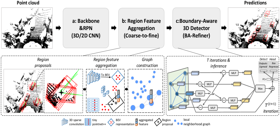
Figure 2: Overview of our proposed BADet. BADet includes three key components: (a) Backbone and Region Proposal Network. We first voxelize the raw point clouds into volumetric grids, resorting to backbone network with a series of 3D sparse convolutions for multi-scale semantic feature abstraction and 3D proposal generation. (b) Region Feature Aggregation Module, which fully exploits multi-level semantic features for more informative RoI-wise representations. (c) Boundary-Aware Graph Neural Network, which takes 3D proposals in immediate neighborhood as inputs for graph construction within a given cut-off distance, associating 3D proposals in the form of local neighborhood graph, with boundary correlations of an object being explicitly informed through an information compensation mechanism.

and sensitive to translation variance. These methods are typically exemplified by PointRCNN [17], which leverages PointNet(++) [21] to segment foreground points from raw point clouds for the purpose of reducing 3D search space, elegantly inheriting the ideology of Faster RCNN [12] architecture. 3DSSD [18] safely removes the core feature propagation layer of PointNet(++) [21] by introducing F-FPS to compensate for the loss of foreground points when downsampling. Point-GNN [19] seeks to generalize graph neural networks (GNNs) to 3D object detection via constructing a graph over downsampled raw point clouds. Few investigations have successfully transplanted GNNs for object detection til Shi et al. proposed Point-GNN [19]. Our BADet differs from Point-GNN by constructing local neighborhood graphs over RoI-wise high semantic features rather than raw point clouds.

Representation learning in hybrid domains. Very recently, a fusion strategy to bring the best of two worlds together is increasingly prevalent. Point-voxel-based methods deeply integrate 3D sparse convolution operation from voxel-based methods and the flexible receptive fields from point-based methods. PVConv [25] demonstrates the effectiveness of the combinations of coarse-grained voxel-wise features and fine-grained point-wise features for synergies. STD [20] voxelizes point-wise features for 3D region proposals and exploits more generic spherical anchors rather than rectangular ones to achieve a high recall and alleviates computational overheads. PV-RCNN [6] leverages set abstraction operation among voxels instead of raw point clouds to achieve flexible receptive fields for fine-grained patterns while maintains computational efficiency. SA-SSD [5] introduces an auxiliary network to consolidate the correlations of 3D feature volumes under the supervision of point-level geometric properties.

3 Proposed BADet

In this section, we propose BADet, which effectively models local boundary correlations of an object by the means of local neighborhood graphs, explicitly facilitating a complete boundary for each individual proposal with an information compensation mechanism. As illustrated in Fig. 2, the proposed BADet network consists of three major components: (a) a backbone followed by a region proposal network (RPN), (b) a region feature aggregation (RFA) module and (c) a boundary-aware graph neural network based 3D object detector (BA-Refiner). Specifically, we first leverage 3D sparse convolutions to extract features from voxelized point clouds. The features are then reshaped to form an BEV representation, which will be fed to the RPN for 3D RoI proposal generation. As for proposal refinement, although the BEV representation is informative (see Sec. 4.4.2), we argue that using it alone suffers from two drawbacks. First, as this representation stems from gradually downsampled 3D feature volumes, the downsampling operation inevitably dilutes the features. Second, with the depth dimension squeezed, the original 3D contextual information is largely lost. To tackle these drawbacks, RFA is introduced to aggregate voxel-wise, pixel-wise, and point-wise features, resulting in enriched RoI-wise features. The RoI features then go through BA-Refiner for a boundary-aware enhancement. Lastly, the enhanced features are fed to a common 3D object detection header to make final detection.

In what follows, we present the backbone and RPN in Sec. 3.1, followed by RFA in Sec. 3.2 and BA-Refiner in Sec. 3.3. Loss functions of BADet are detailed in Sec. 3.4.

3.1 Backbone and Region Proposal Network

3.1.1 Voxelization

We first follow a many-to-one mapping algorithm [5, 15, 14] to voxelize raw point clouds for representation learning. Specifically, let $p$ be a point in a raw point cloud $\mathcal{P}$ with 3D coordinates $\left(p_{x},p_{y},p_{z}\right)$ and reflectance intensities $p_{r}$, where $\mathcal{P}=\left\{p^{i}=\left(p_{x}^{i},p_{y}^{i},p_{z}^{i},p_{r}^{i}\right)\!\in\mathbb{R}^{4}:i=1,...,N\right\}$, $N$ indicates the number of points within $\mathcal{P}$. Let $\left[v_{L},v_{W},v_{H}\right]\in\mathbb{R}^{3}$ be the quantization step, we have the voxelized coordinates of $p$ as $(\lfloor\frac{p_{x}}{v_{L}}\rfloor,\lfloor\frac{p_{y}}{v_{W}}\rfloor,\lfloor\frac{p_{z}}{v_{H}}\rfloor)$, where $\lfloor\cdot\rfloor$ indicates floor function. A voxel $v$ is formed as a set of points that have the same voxelized coordinates. Note that points are stochastically dropped when they exceed the allocated capacity for memory cost saving. Accordingly, a point cloud $\mathcal{P}$ is positioned into a feature map with a resolution of $L\times W\times H$, subject to the quantization step $\left[v_{L},v_{W},v_{H}\right]$. Following [15, 6], we obtain the initial feature representation per voxel, denoted by $f(v)$, as the mean of its points, i.e. $f(v)=\frac{1}{|v|}\sum_{p\in v}(p_{x},p_{y},p_{z},p_{r})$.

3.1.2 Network architecture

As shown in Figure 2, we follow the architecture in [14, 15, 5] to employ 3D backbone and 2D backbone networks to summarize features for BADet. 3D backbone network [16, 6] jointly downscales 3D feature volumes by half from point clouds with a series of stacked 3D sparse convolutions and sub-manifold convolutions, each of which follows a batch normalization and non-linear ReLU function. 2D backbone network simply stacks six standard convolutions with kernel size of 3 $\times$ 3, to convolve against 2D bird-view feature maps reshaped from the output of 3D backbone network for further feature abstraction. Our detection header comprises two sibling 1 $\times$ 1 standard convolutions, generating high-quality 3D proposals in a pixel-by-pixel fashion for the following graph construction (see Sec. 4.1.2).

3.2 Region Feature Aggregation

The art of feature aggregation for RoI-wise representation is of significance (see Sec. 4.4.2). As aforementioned, BEV representation is informative. Nevertheless, such an underlying mechanism induces information loss, which degrades more accurate localization. Instead, by aggregating voxel-wise, pixel-wise, and point-wise feature together, we achieve the top performance. In a sequel, we specify the details of each feature component.

3.2.1 Voxel-wise feature encoding

To obtain voxel-wise feature, we introduce auxiliary branches to jointly optimize voxel-wise features from 3D backbone network. Specifically, we restore the real-world 3D coordinates for each voxel from nonzero indices on the basis of a quantization step at current stage, together with its corresponding 3D sparse convolution features, i.e. each voxel is in the form of $\left\{\left(\mathbf{f}_{j},p_{j}\right):j=1,...,M\right\}$, where $\mathbf{f}_{j}$ denotes 3D sparse convolution feature and $p_{j}$ indicates the real-world coordinates of a voxel centroid. To associate multi-scale features from different stages, we gradually broadcast these 3D sparse convolution features into raw point clouds via feature propagation algorithm mentioned in [21]. As the resolution of 3D sparse convolution features decreases, background points close to object’s boundary are likely to be mistaken for foreground points, and consequently mislead the model. To enable our voxel-wise features to be more aware of the object’s boundary, we add an auxiliary header to the interpolated 3D sparse convolution features of raw point clouds, jointly optimizing foreground segmentation and relative center offset estimation by point-wise supervisions. After that, we throw the auxiliary header away, and then interpolate 3D sparse convolution features $\mathbf{f}^{\left(voxel\right)}$ of raw point clouds from the neck, which compensates for the information loss of directly converting 3D sparse convolution feature map into 2D BEV representation without ever restoring its 3D structure context.

3.2.2 Pixel-wise feature encoding

To obtain our pixel-wise feature, we interpolate grid point features from the nearest pixel along channels from BEV representation, which is considered as a variant of RoIAlign operation adapted from SA-SSD [5]. Specifically, for each 3D proposal, we generate $m_{1}\times m_{2}$ evenly spaced mesh grids along $x$- and $y$-axes in the BEV perspective of a 3D proposal, respectively. Note that $m_{1}$ and $m_{2}$ are two user-specified constants which are subject to aspect ratio of a certain category. We then encode BEV representation into $m_{1}\times m_{2}$ feature maps. For each mesh grid point, we interpolate one position over a single feature map via spatial transformer sampler [26] to form the final pixel-wise feature component $\mathbf{f}^{\left(pixel\right)}\in\mathbb{R}^{m_{1}\cdot m_{2}}$ of RoI-wise representation at negligible cost. Pixel-wise feature can be extracted by any traditional RoIAlign operations in practice. Whereas, traditional pooling mechanism suffers from expensive computation overheads.

3.2.3 Point-wise feature encoding

To compensate for the information loss induced by quantization error [6, 18], we employ an adapted PointNet(++) [21] variant. As we leverage the commonly used backbone [14, 15, 16] to gradually 8 times downsample 3D feature volumes for the purpose of memory usage saving, which dilutes 3D features inevitably. We therefore train a tiny PointNet from scratch, which consumes raw point clouds as inputs to summarize the whole scene into a fraction of keypoints’ semantic features, which are then broadcast into the centroids of the proposed 3D proposals to obtain point-wise feature component, $\mathbf{f}^{\left(point\right)}$, with the help of feature propagation algorithm in [21].

Finally, we summarize the three aforementioned multi-level associated feature components via concatenation to enrich the final RoI-wise representations for graph construction in the stage two, which significantly contributes to the performance (see Sec. 4.4.4) as

$$\text{X}\!=\!\left\{\mathbf{x}_{i}\!=\!\left(x_{i},\!\left[\mathbf{f}_{i}^{\left(voxel\right)},\mathbf{f}_{i}^{\left(pixel\right)},\mathbf{f}_{i}^{\left(point\right)}\right]\right)\!\!:i\!=\!1,...,n\right\}.$$ (1)

3.3 Boundary-Aware 3D Detector

In this section, we describe our boundary-aware 3D detector. We assume that we have already obtained 3D proposals and their corresponding RoI-wise representations. We first describe how the graph is constructed (see Sec. 3.3.1). We then detail graph update algorithm (see Sec. 3.3.2).

3.3.1 Graph construction

Consider an $(F+3)$-dimensional detection set with $n$ 3D proposals, denoted by $\text{X}=\left\{\mathbf{x}_{1},...,\mathbf{x}_{\mathbf{n}}\right\}\subseteq\mathbb{R}^{F+3}$, where $\mathbf{x}_{i}=(x_{i},\mathbf{s}_{i})$ is regarded as a node of graph $\mathcal{G}$ with 3D coordinates $x_{i}\in\mathbb{R}^{3}$ and initial node state $\mathbf{s}_{i}\in\mathbb{R}^{F}$. Note that coordinates $x_{i}$ represents the centroid of a detected 3D proposal and the node state $\mathbf{s}_{i}$ is initialized accordingly by the RoI-wise representation extracted and aggregated from the corresponding region. In our case, we construct local neighborhood graph $\mathcal{G}\left(\mathcal{V},\mathcal{E}\right)$ of X in $\mathbb{R}^{F+3}$ as

$$\mathcal{E}=\left\{(i,j)|\lVert x_{i}-x_{j}\rVert_{2}<r\right\},$$ (2)

where $\mathcal{V}=\left\{1,...,n\right\}$ and $\mathcal{E}\subseteq\mathcal{V}\times\mathcal{V}$ are the nodes and edges, respectively, $r$ is the given cut-off threshold. $\mathcal{G}\left(\mathcal{V},\mathcal{E}\right)$ is undirected, which includes self-loop, meaning each node connects to itself. In this work, we define $\mathcal{N}\left(i\right)$ as neighborhood function, which draws neighbors from the set $\left\{j\in\mathcal{V}\ :\ \left(i,\ j\right)\in\mathcal{E}\right\}$ with a runtime complexity $O\left(c\left|\mathcal{V}\right|\right)$ in the worst case, where $c$ is an user-specified constant.

3.3.2 Graph update

The vanilla graph update algorithm. The main idea described in Algorithm 1 is that each node of $\mathcal{G}(\mathcal{V},\mathcal{E})$ updates itself via aggregating information from their immediate neighbors at the previous iteration. As information flows over nodes, each node gradually gains an expanding receptive field from further reaches of its neighbors. As we have illustrated in Sec. 1, 3D proposals X that generated by region proposal network usually offset from ground truth somehow, emerging in local neighborhood densely with an underlying probability. In fact, only a handful of proposals should fully cover the regions where objects truly exist.

Input: Graph $\mathcal{G}(\mathcal{V},\mathcal{E})$; input features $\{\mathbf{x}_{i},\forall i\in\mathcal{V}\}$; depth $K$; weight matrices $\mathbf{W}^{k}_{g},\mathbf{W}^{k}_{f}$, $\forall k\in\{1,\cdots,K\}$; non-linearity $\sigma$; channel-wise symmetric aggregator function ${\Box}_{k}\left(\text{\emph{e.g}.\hbox{} missing}\ \Sigma\ \text{or\ }\max\right),\forall k\in\{1,\cdots,K\}$; concatenation function: $CAT$ along aixs $1$ dimension; neighborhood function $\mathcal{N}:i\to 2^{\mathcal{V}}$.

Output: Vector representations $\mathbf{z}_{i}$ for all $i\in\mathcal{V}$.

1 $\mathbf{h}_{i}^{0}\leftarrow\mathbf{x}_{i},\forall i\in\mathcal{V}$;

2 for $k=1\dots K$ do

3       for $i\in\mathcal{V}$ do

4             $\mathbf{h}_{\mathcal{N}\left(i\right)}^{k}\leftarrow\!\Box_{k}\!\left(\mathbf{W}^{k}_{g}\!\cdot\!CAT\!\left(\!\{\mathbf{h}_{j}^{k-1},\forall j\in\mathcal{N}\left(i\right)\}\!\right)\!\right)$;

5             $\mathbf{h}_{i}^{k}\leftarrow\mathbf{h}_{i}^{k-1}+\sigma\left(\mathbf{W}^{k}_{f}\cdot\mathbf{h}_{\mathcal{N}\left(i\right)}^{k}\right)$;

6            

7       end for

8      

9 end for

$\mathbf{z}_{i}\leftarrow\mathbf{h}_{i}^{K},\forall i\in\mathcal{V}$.

Algorithm 1 The vanilla graph update algorithm

More often than not, proposals X we obtained can deviate somehow in cases where azimuth or $x_{i}$ offsets from the ground truth. As a result, when we extract and aggregate semantic features from these proposed regions to summarize RoI-wise representations for refinement, a proportion of the boundary information of an object is naturally lost. Under existing coarse-to-fine paradigms, RoI-wise representations are treated individually as uncorrelated entries when fed to following detection headers, each of which alone fails to perceive a complete boundary of an object by itself. In our case, we model local boundary correlations of an object in the form of local neighborhood graph to exploit the spatial correlations among the RoI proposals so that each of them will possess the whole receptive field of the associated object, i.e. “boundary aware", by taking the semantic features from further reaches of its neighbors into account. As described in Algorithm 1, $k$ in the outer loop represents the current step, $\mathbf{h}_{k}$ indicates the hidden state of a node at present step. In the vanilla version, $\left\{\mathbf{h}_{j}^{k-1},\forall j\in\mathcal{N}\left(i\right)\right\}$ denotes associated feature vectors of the local neighbors of node $i\in\mathcal{V}$, which is directly concatenated before fed through a multi-layer perceptron network (MLP) for feature transformation. We then aggregate these transformed features into a single vector, $\mathbf{h}_{\mathcal{N}\left(i\right)}^{k}$, via aggregation operator. In this paper, we adopt $\max\left(\cdot\right)$ aggregator inspired by rencent advances in leveraging graph neural network to learn feature representations over point sets [19].

The extended graph update algorithm. To alleviate translation variance mentioned in [18, 19], we extend our graph propagation strategy via concatenating the relative offset $x_{i}-x_{j}$ to the semantic feature of each node $j\in\mathcal{V}$. Note that node $j$ is from further reaches of node $i$’s neighbors, where $i\in\mathcal{V}$ is the central node. Also, given $\mathbf{x}_{i}$ already contains local structure context from previous iteration, we follow [19] to predict an alignment offset $\varDelta x_{i}^{k}$ for each node in $\mathcal{N}\left(i\right)$. These alignment offsets are insensitive to slight disturbances or jitteriness, and thus lead to more robust detection outcomes. Let $\left[\cdot\right]$ be an element-wise concatenation and thus the final aggregated feature in this paper is obtained by as

$$\mathbf{h}_{\mathcal{N}\left(i\right)}^{k}\!\!\!\leftarrow\!\max_{k}\!\left(\!\mathbf{W}_{g}^{k}\!\cdot\!CAT\!\left(\!\left\{\!\left[x_{i}\!-\!x_{j}\!-\!\varDelta x_{i}^{k};\mathbf{h}_{j}^{k-1}\right]\!,\!\forall j\!\in\!\mathcal{N}\left(i\right)\!\right\}\!\right)\!\right).$$ (3)

3.3.3 Graph header

We introduce two sibling branches, which takes $\mathbf{z}_{i}$ as inputs with two stacked MLP layers for refinement: one is for bounding box classification, and the other is for more accurate oriented 3D bounding box regression (see Figure 2).

3.4 Loss Functions

To learn informative representations in a fully supervised fashion, we follow the conventional anchor-based settings in [15]. In particular, we use Focal Loss [13], Smooth-L1 Loss for the bounding box classification and regression in both stage one ($\mathcal{L}_{rpn}$) and stage two ($\mathcal{L}_{gnn}$), respectively. To obtain better boundary-aware voxel-wise representations described in Sec. 3.2.1, we introduce a center offset estimation branch as

$$\mathcal{L}_{offset} \!=\!\frac{1}{N_{pos}}\sum_{i}^{N}{\mathcal{L}_{\text{smooth}-\text{L}1}\!\left(\!\varDelta\hat{d}\!-\!\varDelta d^{*}\!\right)\!\cdot\!\mathbbm{1}\left[b_{i}^{*}\geq 1\right]},$$ (4)

where $\varDelta d^{*}$ indicates the offsets of interior points of a ground-truth bounding box from center coordinates, $N_{pos}$ represents the number of foreground points, $\mathbbm{1}\left[b_{i}^{*}\geq 1\right]$ indicates only the points fall in ground-truth bounding box are considered. Besides, we summarize foreground segmentation loss as

$$\mathcal{L}_{seg} =\frac{1}{N_{pos}}\sum_{i}^{N}{-}\alpha\left(1-\hat{p}_{i}\right)^{\gamma}\log\left(\hat{p}_{i}\right),$$ (5)

where $\hat{p}_{i}$ indicates the predicted foreground probability. The overall loss $\mathcal{L}$ is formulated as

$$\mathcal{L}=\mathcal{L}_{rpn}+\mathcal{L}_{gnn}+\mathcal{L}_{offset}+\mathcal{L}_{seg}.$$ (6)

4 Evaluation

In this section, we introduce experimental setup of BADet, including dataset, network architecture, as well as training and inference details (Sec. 4.1). We report comparisons with the existing state-of-the-art approaches on both the widely used KITTI Dataset (Sec. 4.2) and highly challenging nuScenes Dataset 4.3. In Sec. 4.4, extensive ablation studies are conducted on KITTI Dataset in diverse evaluation settings to investigate the effectiveness of each component of BADet. Also, we report runtime analysis for future optimization (Sec. 4.5).

4.1 Experimental Setup

4.1.1 Dataset

KITTI Dataset [27, 28] contains 7,481 training samples and 7,518 testing samples for three categories (i.e. $Car$, $Pedestrian$, and $Cyclist$) in the context of autonomous driving, each of which has three difficulty levels (i.e. $Easy$, $Moderate$, and $Hard$) according to object scale, occlusion, and truncation levels. As a common practice mentioned in [29], we evaluate our proposed BADet on the KITTI 3D and BEV object detection benchmark following the frequently used train, val split, with 3,712, 3,769 annotated samples for training, validation, respectively. Following previous literature [5, 7], we report the performance of the most commonly-used car category for fair comparison on both the val split and the test split by submitting to the online learderboard.

nuScenes Dataset [30] consists of 1000 challenging driving sequences, each of which is about 20-second long, with 30k points per frame. It totally annotates 1.17M 3D objects on 10 different classes with 700, 150, 150 annotated sequences for train, val and test split, respectively. In particular, 28k key frames are annotated for train split, and 6k, 6k for val and test split accordingly. To predict velocity, existing methods concatenate lidar points from key frame and frames in last 0.5-second together, resulting in approximately 400k points in total. Following previous literature [18], we train BADet on train split and compare with the state-of-the-art methods on val split to further confirm the validity of the proposed method.

4.1.2 Network Architecture

As shown in Figure 3, we follow the architecture in [14, 15, 5] to design 3D backbone and 2D backbone network for BADet. 3D backbone network downsamples 3D feature volumes from point clouds with dimensions 16, 32, 64, 64, respectively, each of which comprises a series of 3 $\times$ 3 $\times$ 3 sub-manifold sparse convolutions, together with a batch normalization and non-linear ReLU following each convolution. 2D backbone network stacks six standard 3 $\times$ 3 convolutions, of which filter number is 256, to convolve against 2D bird-view feature map reshaped from the output of 3D backbone network for further feature abstraction. The detection header is composed of two sibling 1 $\times$ 1 convolutions with filter numbers of 256, which generates high-quality 3D proposals for graph construction in the second stage. As for region feature aggregation module, we use MLPs of unit (32+64+64, 64) for feature transformation, followed by two branches of units (64, 1), (64, 3) for foreground classification and center offset estimation. Also, we train a lightweight tiny PointNet-like block from scratch, of which two neighboring radii of each level are set as (0.1m, 0.5m), (0.5m, 1.0m), (1.0m, 2.0m), respectively. The keypoints sampled for each level is set to 4,096, 1,024, 256 via FPS algorithm [21]. Finally, with regard to boundary-aware 3D detector, we stack three MLPs of units (64+28+28, 60, 30, 120) with ReLU non-linearity for computating edges and updating nodes of local neighborhood graphs.

4.1.3 Training

Our BADet consumes regular voxels as input. For KITTI Dataset, we first voxelize the raw point clouds with a quantization step of [0.05m, 0.05m, 0.1m]. Note that only objects in FOV are annotated for KITTI Dataset, we follow [16, 7, 5] to clip the range of point clouds into [0, 70.4]m, [-40, 40]m, and [-3, 1]m along the x, y, z axes, respectively. The resolution of final BEV feature map is 200 $\times$ 176. Hence, a total of 200 $\times$ 176 $\times$ 2 pre-defined anchors (width=1.6m, length=3.9m, height=1.56m) for car category are evenly generated, with two possible orientations ($0^{\circ}$ or $90^{\circ}$) being considered. These anchors are subject to the averaged dimensions over the whole KITTI Dataset. Furthermore, we follow the matching strategy of VoxelNet[14] to distinguish the negative and positive anchors with IoU thresholds 0.45 and 0.6, respectively. For nuScenes Dataset, the detection range is within [-54, 54]m for the x axis, [-54, 54]m for the y axis and [-5, 3]m for z axis, with a quantization step of [0.075m, 0.075m, 0.2m] along each axis. Given that nuScenes Dataset has 10 classes with a large variance on scale, we therefore use multiple seperated regression heads for region proposals generation in the first stage.

The whole architecture of our BADet is optimized from scratch in an end-to-end fashion. For KITTI Dataset, we optimize the entire network with batch size 2, weight decay 0.001 for 50 epochs with the SGD optimizer on a single GTX 1080 Ti GPU. The learning rate is initialized with 0.01, which is decayed with a cosine annealing strategy adopted in SA-SSD [5]. During training, we consider frequently adopted data augmentations to facilitate our BADet’s generalization ability, including global rotation around $z$-axis with the noise uniformly drawn from $\left[-\frac{\pi}{4},\frac{\pi}{4}\right]$, global scaling with

Table 1: Performance comparison with state-of-the-arts on KITTI test server. We report the Average Precision(AP) with 40 recall positions on both BEV and 3D object detection leaderboard of $Car$ category with a rotated IoU threshold 0.7. The top performance is indicated in bold. Please refer to http://www.cvlibs.net/kitti/eval_object?benchmark=3d for the purpose of online validation.

Method	$AP_{3D}\left(\%\right)$			$AP_{BEV}\left(\%\right)$
	Easy $\downarrow$	Mod. $\downarrow$	Hard $\downarrow$	Easy $\uparrow$	Mod. $\uparrow$	Hard $\uparrow$
VoxelNet[14], CVPR18	77.82	64.17	57.51	87.95	78.39	71.29
SECOND[15], Sensors18	83.34	72.55	65.82	89.39	83.77	78.59
PointPillars[16], CVPR19	82.58	74.31	68.99	90.07	86.56	82.81
Point-GNN[19], CVPR20	88.33	79.47	72.29	93.11	89.17	83.90
3DSSD[18], CVPR20	88.36	79.57	74.55	92.66	89.02	85.86
SA-SSD[5], CVPR20	88.75	79.79	74.16	95.03	91.03	85.96
MV3D[29], CVPR17	74.97	63.63	54.00	86.62	78.93	69.80
ContFuse[31], ECCV18	83.68	68.78	61.67	94.07	85.35	75.88
F-PointNet[32], CVPR18	82.19	69.79	60.59	91.17	84.67	74.77
AVOD-FPN[33], IROS18	83.07	71.76	65.73	90.99	84.82	79.62
PointRCNN[17], CVPR19	86.96	75.64	70.70	92.13	87.39	82.72
MMF[34], CVPR19	88.40	77.43	70.22	93.67	88.21	81.99
3D-CVF[35], ECCV20	89.20	80.05	73.11	93.53	89.56	82.45
3D IoU Loss[36], 3DV19	86.16	76.50	71.39	91.36	86.22	81.20
Part-A2[37], TPAMI20	87.81	78.49	73.51	91.70	87.79	84.61
STD[20], ICCV19	87.95	79.71	75.09	94.74	89.19	86.42
PV-RCNN[6], CVPR20	90.25	81.43	76.82	94.98	90.65	86.14
Voxel R-CNN[38], AAAI21	90.90	81.62	77.06	94.85	88.83	86.13
BADet	89.28	81.61	76.58	95.23	91.32	86.48

Table 2: Performance comparison with state-of-the-arts on val set. We report the Average Precision(AP) with 11 recall positions on 3D object detection leaderboard of $Car$ category with a rotated IoU threshold 0.7. The top performance is indicated in bold.

Method	$AP_{3D}\left(\%\right)$
	Easy $\downarrow$	Moderate $\uparrow$	Hard $\downarrow$
SECOND[15], Sensors18	87.43	76.48	69.10
PointPillars[16], CVPR19	-	77.98	-
PointRCNN[17], CVPR19	88.88	78.63	77.38
3DSSD[18], CVPR20	89.71	79.45	78.67
CIA-SSD[7], AAAI21	90.04	79.81	78.80
SA-SSD[5], CVPR20	90.15	79.91	78.78
MV3D[29], CVPR17	71.29	62.68	56.56
F-PointNet[32], CVPR18	83.76	70.92	63.65
ContFuse[31], ECCV18	86.32	73.25	67.81
AVOD-FPN[33], IROS18	84.41	74.44	68.65
Fast Point R-CNN[39], ICCV19	89.12	79.00	77.48
STD[20], ICCV19	89.70	79.80	79.30
PV-RCNN[6], CVPR20	-	83.90	-
Voxel R-CNN[38], AAAI21	89.41	84.52	78.93
BADet	90.06	85.77	79.00

the scaling factor uniformly drawn from [0.95, 1.05], and global flipping along $x$-axis simultaneously. Also, we adopt a grond-truth augmentation strategy proposed by SECOND [15] to enrich the current training scene by seamlessly “pasting” a handful of new ground-truth boxes and the associated points that fall in them. For the nuScenes Dataset, we optimize the entire network with batch size 2, weight decay 0.01 for 7 epochs with the ADAM optimizer on two GTX 1080 Ti GPUs. We adopt the one cycle learning rate strategy with default settings, where the maximum learning rate is 0.001.

4.1.4 Inference

For KITTI Dataset, we select high-confidence bounding boxes with a threshold 0.3. We use non-maximum suppression (NMS) with a rotated IoU threshold 0.1 to remove redundancy. Please refer to BADet’s source code for more details since we will enclose herewith implementation details.

4.2 3D Detection on the KITTI Dataset

To evaluate the performance of BADet on val set, we utilize the train split for training. To fairly evaluate the proposed BADet’s performance on test set, of which the labels are unavailable, we train on all train+val data and use the parameters of last epoch for online test server submission.

4.2.1 Evaluation Metric

We follow KITTI Dataset protocal by using Interpolated AP@$S_{N}$ Metric, which indicates the mean precision of N equally spaced recall levels as

$$\text{AP}=\frac{1}{N}\sum_{r\in S}{P_{interpolate}\left(r\right)},$$ (7)

where $S=\left[q_{0},q_{0}+\frac{q_{1}-q_{0}}{N-1},q_{0}+\frac{2\left(q_{1}-q_{0}\right)}{N-1},...,q_{1}\right]$ is a subset for N recall levels, of which the precision interpolated for each recall level $r$ is represented by

$$P_{interpolate}\left(r\right)=\underset{\tilde{r}:\tilde{r}\geq r}{\max}\ P\left(\tilde{r}\right).$$ (8)

As a common practice, we report average precision (AP) with a rotated IoU threshold 0.7 for $Car$ in terms of assessing the quality of our proposed BADet. From 08.10.2019, KITTI benchmark adopts the Interpolated AP@$S_{40}$ Metric with 40 recall levels $S_{40}=\left[1/40,2/40,3/40,...,1\right]$ as suggested in [40] for more fair evaluation. We follow the conventions as previous works [5, 6, 7] do. We evaluate on the $test$ set by submitting to online $test$ server of which 40 recall positions are considered. We evaluate on $val$ set with 11 recall positions $S_{11}=\left[0,0.1,0.2,...,1\right]$ to compare with existing state-of-the-arts unless otherwise noted.

4.2.2 Comparison with State-of-the-Arts

We compare the performance of our BADet on the KITTI test set with previous state-of-the-art methods by submitting predictions to the official online leaderboard [28, 27]. As shown in Table 1, Our BADet outperforms all its competitors with remarkable margins on KITTI BEV detection leaderboard and ranks $1^{st}$ on $Car$ category of $Moderate$ difficulty, surpassing the second place, SA-SSD [5] by $\left(0.2\%,0.29\%,0.52\%\right)$ for Easy, Moderate, and Hard level respectively as of Apr. 17th, 2021. Note that our backbone network at the first stage is built upon the architecture of SA-SSD while obtains an absolute gain by (0.53%, 1.82%, 2.42%) on 3D detection benchmark. To the best of our knowledge, little literature has achieved decent performance on 3D object detection via leveraging graph neural network until Point-GNN [19] is proposed. We surpass Point-GNN (0.95%, 2.14%, 4.29%) on 3D detection benchmark, (2.12%, 2.15%, 2.58%) on BEV detection benchmark while keep nearly 5 times faster than Point-GNN (7.1 FPS vs. 1.5 FPS). Compared with the latest state-of-the-art Voxel R-CNN [38], our BADet is slightly lower (-0.01%) but remains close on 3D detection benchmark while achieves (0.38%, 2.49%,, 0.35%) improvement on BEV detection benchmark. Note that we outperform Voxel R-CNN by 2.49% on Car category of Moderate difficulty. Figure 4 further indicates better detection coverage of our BADet with different recall settings. Furthermore, we visualize some predictions from test set for qualitative comparison in Figure 3.

In addition, as shown in Figure 2, we exploit Interpolated AP@$S_{11}$ Metric with a rotated IoU threshold 0.7 for further comparison with previous works on val set. Besides, by considering the results in Table 1, 2, we argue that such slightly inconsistent result between val set and test set plausibly can be reduced to the mismatched data distributions, as Part-$A^{2}$ [37] notes.

Overall, our BADet achieves decent performance on both val set and test set, which consistently demonstrates the effectiveness of our boundary-aware 3D detector.

4.3 3D Detection on the nuScenes Dataset

To further confirm the validity of the proposed method, we evaluate the performance of BADet on the highly challenging large-scale nuScenes Dataset.

4.3.1 Evaluation Metric

We follow nuScenes Dataset protocal by using mean Average Precision (mAP) and nuScenes detection score (NDS) as the main evaluation metrics for 3D object detection. The mAP assesses a bird-eye-view center offset within cut-off distances 0.5m, 1m, 2m, 4m rather than a standard Intersection over Union (IoU). Let $E=\{mATE,\ mASE,\ mAOE$ $,\ mAAE,\ mAVE\}$ be a set of the mean average errors of translation, size, orientation, attribute and velocity, the NDS denotes a weighted average metric, which is obtained by

$$NDS=\frac{1}{10}\left[5mAP+\sum_{err\in E}{\left(1-\min\left(1,\ err\right)\right)}\right].$$ (9)

4.3.2 Comparison with State-of-the-Arts

Table 3 and Table 4 reveal that our BADet outperforms 3DSSD[18] remarkably with 4.99%, 2.44% gains for mAP, NDS, respectively. Also, Table 3 shows that BADet surpasses the existing state-of-the-art approaches remarkably among most categories except for 3D $Car$, $Bus$, $Truck$, $Trailer$, $Construction\ vehicle$ detection, where the top three gains are 27.14%, 18.47%, 10.03% for 3D $traffic\ cone$, $Bicycle$, $Pedestrian$ detection, which again validates the effectiveness of our region feature aggregation module in terms of aggregating informative contextual information, especially for small object detection. All results reported on the large-scale nuScenes Dataset further demonstrate the validity of the proposed method.

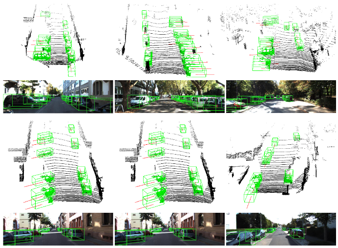
Figure 3: Qualitative results on KITTI test set using BADet. The predicted bounding boxes of Cars (in green) are drawn on both the point cloud ($1^{st}$ & $3^{rd}$ ) and the image ($2^{nd}$ & $4^{th}$). Best view in color.

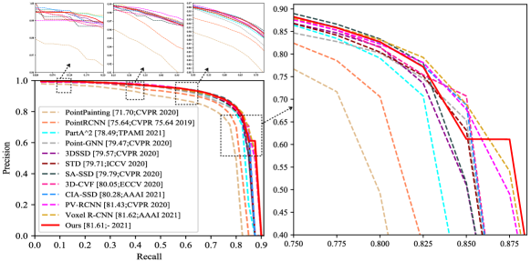
Figure 4: Precision $\times$ Recall curve of state-of-the-art methods on online KITTI 3D detection benchmark. We report average precision (AP) with a rotated IoU threshold 0.7 for Moderate difficulty of Car category.

4.4 Ablation Study

In this section, comprehensive ablation experiments are conducted to analyze the effectiveness of each component of our proposed BADet. Note that we report all results by Interpolated AP@$S_{11}$ Metric with a IoU threshold 0.7 unless otherwise noted. We train all our models on the train set and evaluate on the val set for the most important Moderate difficulty of Car category of KITTI Dataset [28, 27].

4.4.1 Effect of region feature aggregation

To judiciously verify the effectiveness of our region feature aggregation module, we disable RFA module by directly adding a commonly used detect head on the top of the 2D backbone network in the SA-SSD [5]. As illustrated in the $2^{nd}$, $3^{rd}$ rows of Table 5, our RFA module typically integrates multi-grain semantic features in a coarse-to-fine manner and further improves the performance by (0.16%, 0.13%, 0.02%) on all the three subsets.

4.4.2 Effect of different feature components for RFA module

We closely verify each level feature component of RoI-wise representations in Eq. (1) by controlled experiments. As shown in the $1^{st}$, $2^{nd}$, and $3^{rd}$ rows of Table 6, the performance of BADet deteriorates a lot when $\mathbf{f}^{\left(pixel\right)}$ from BEV representation is absent. Nevertheless, it can not achieve state-of-the-art performance by itself.

Table 3: Performance of different models on nuScenes, measured by the mean Average Precision (mAP). Numbers of SECOND, PointPillars and 3DSSD are cited from [18].

Methods	Car $\downarrow$	Ped $\uparrow$	Bus $\downarrow$	Barrier $\uparrow$	TC $\uparrow$	Truck $\downarrow$	Trailer $\downarrow$	Moto $\uparrow$	Cons.Veh. $\downarrow$	Bicycle $\uparrow$	mAP $\uparrow$
SECOND[15]	75.53	59.86	29.04	32.21	22.49	21.88	12.96	16.89	0.36	0	27.12
PointPillar[16]	70.50	59.90	34.40	33.20	29.60	25.00	20.00	16.70	4.50	1.60	29.50
3DSSD[18]	81.20	70.17	61.41	47.94	31.06	47.15	30.45	35.96	12.64	8.63	42.66
BADet	80.30	80.20	57.10	57.50	58.20	43.70	25.00	36.00	11.40	27.10	47.65

Table 4: Performance of different models on nuScenes, measured by the nuScenes Detection Score (NDS). Numbers of PointPillars and 3DSSD are cited from [18].

	mAP $\uparrow$	mATE $\downarrow$	mASE $\downarrow$	mAOE $\downarrow$	mAVE $\uparrow$	AAE $\uparrow$	NDS $\uparrow$
PointPillars [16]	29.50	0.54	0.29	0.45	0.29	0.41	44.90
3DSSD [18]	42.66	0.39	0.29	0.44	0.22	0.12	56.40
BADet	47.65	0.30	0.27	0.34	0.41	0.18	58.84

Table 5: Effect of region feature aggregation module and boundary-aware 3D detector. Here, “SA-SSD”, “RFA”, “BEV-Header”, and “BA-Refiner” denote the original architecture claimed in [5], region feature aggregation module, the commonly used detect head and our boundary-aware 3D detector with a detect head, respectively.

Components				$AP_{3D}\left(\%\right)$			$AP_{BEV}\left(\%\right)$
SA-SSD	RFA	BEV-Header	BA-Refiner	Easy	Mod.	Hard	Easy	Mod.	Hard
✓				90.04	79.78	78.91	90.64	89.12	80.49
✓		✓		89.93	79.81	78.83	90.65	88.68	87.95
✓	✓	✓		90.09	79.94	78.85	90.66	88.76	88.05
✓	✓		✓	90.06	85.77	79.00	90.63	88.86	88.10

Table 6: Effect of each feature component of region feature aggregation module.

Components			$AP_{3D}\left(\%\right)$			$AP_{BEV}\left(\%\right)$
$f^{\left(pixel\right)}$	$f^{\left(voxel\right)}$	$f^{\left(point\right)}$	Easy	Mod.	Hard	Easy	Mod.	Hard
✓			90.00	79.93	78.88	90.60	88.87	88.04
	✓		87.85	76.24	72.96	89.60	82.83	78.73
		✓	88.36	76.96	74.10	89.87	83.62	79.09
	✓	✓	88.58	77.88	75.37	89.93	84.65	79.48
✓		✓	90.07	79.95	78.93	90.62	88.90	88.08
✓	✓		89.99	80.00	78.97	90.57	88.96	88.07
✓	✓	✓	90.06	85.77	79.00	90.63	88.86	88.10

This is because the progressive downsampled 3D feature volumes and the absence of 3D structure context when converting to BEV representation directly may degrade its localization accuracy. The aggregation of $\mathbf{f}^{\left(pixel\right)}$, $\mathbf{f}^{\left(voxel\right)}$, and $\mathbf{f}^{\left(point\right)}$ significantly benefits the performance as shown in the $5^{th}$ to $7^{th}$ rows. Note that each level feature component of $\mathbf{x}$ shows a supplementary effect more than a superposition. As shown in the last row, the aggregation of all feature components contributes to the top performance with 85.77% AP on the Moderate difficulty of Car category.

4.4.3 Effect of boundary-aware 3D detector

As illustrated in the $3^{rd}$, $4^{th}$ rows of Table 5, our boundary-aware 3D detector raises the moderate AP (by 5.81%), and hard AP (by 0.13%) for KITTI car category of 3D detection and boosts the easy (by 0.11%), moderate (by 0.12%) and hard (0.08%) categories of BEV detection without bells and whistles. The substantial improvements bring us a strong baseline, which validates that our proposed module could learn much richer boundary-aware contextual information in a coarse-to-fine manner by directly taking the semantic features from further reaches of its neighbors into account.

4.4.4 Effect of boundary-aware 3D detector with T iterations

We propose boundary-aware 3D detector in Sec. 3.3 to model local boundary correlations of an object. Since graph neural network updates its nodes iteratively, the number of iterations is an important hyper-parameter. As shown in Table 7, the $1^{st}$ row shows the nodes’ state initialized by $\mathbf{x}$ can not achieve the top performance without our information compensation mechanism. Note that the performance is significantly improved as the receptive field is expanding via graph edges with $T$ iterations. We set $T$ to 3 for online test server submission. Whereas, for val set, $T$=4 achieves the best performance. Particularly, when $T$ is set to 5, the performance drops dramatically, which is likely due to the problem of gradient vanishing.

Table 7: Ablation study on the KITTI val set with T iterations of BADet.

Number of	$AP_{3D}\left(\%\right)$			$AP_{BEV}\left(\%\right)$
iterations	Easy	Mod.	Hard	Easy	Mod.	Hard
T=0	90.06	79.94	78.85	90.66	88.76	88.05
T=1	85.68	80.16	77.84	88.72	88.13	87.76
T=2	89.24	83.11	78.91	90.15	88.63	87.99
T=3	90.06	85.77	79.00	90.63	88.86	88.10
T=4	90.28	85.79	79.11	90.71	88.97	88.17
T=5	90.02	79.87	78.85	90.65	88.83	88.11

Table 8: Runtime analysis for each component during inference stage. ms indicates millisecond.

Components	RPN	RFA	BA-Refiner	NMS	Overall
Avg. time (ms)	43.65	26.73	61.98	1.49	140.36

4.5 Runtime Analysis

The inference time is important for the deployment of downstream applications in the context of autonomous driving. Hence, we report a breakdown of runtime of our BADet for future optimization 8. Our BADet is implemented by Pytorch with Python language. We set batch size to 1 and assess runtime on a single Intel(R) Core(TM) i7-6900K CPU and a single GTX 1080 Ti GPU. The average inference time (in millisecond) over val set (3769 samples) of BADet is 140.36 ms, which is almost five times faster than Point-GNN [19] (7.1 FPS vs. 1.5 FPS): As show in Table 8, (i) 3D proposal generation in the first stage takes 43.65ms (31.10%); (ii)Region feature aggregation network takes 26.73ms (19.04%); (iii) boundary-aware graph neural network takes 61.98ms (44.16%); and non-maximum suppression for filtering redundancy takes 1.49ms (1.04%). In fact, as She et al. notes [19], factors affecting the runtime varies from software level (e.g. code optimization) to hardware level (e.g. GPU resources). Optimizing runtime is out of the scope of this paper. However, an analysis of inference time facilitates more follow-up works in this field.

5 Concluding Remarks

We have presented BADet for 3D object detection from point clouds. Conceptually, the new model provides an information compensation mechanism to deal with the situation wherein RoI proposals lack enough information about the object boundary due to their deviations to the (unknown) ground truth. Extensive experiments on two public benchmarks, i.e. the widely acknowledged KITTI and the more recent nuScenes, show that BADet compares favorably against the state-of-the-art. The encouraging results can set a new baseline for more follow-up literature and are poised to facilitate other downstream applications.

Much remains to be done. First, the inference time needs to be further optimized, say by down-scaling the

Table 9: Comparing the runtime speed of our BADet with state-of-the-art detectors.

Methods	PointRCNN	Part-$A^{2}$	STD	PV-RCNN	Point-GNN	BADet
Speed (FPS)	10	12.5	12.5	12.5	1.5	7.1

local neighborhood graphs. Second, attention mechanisms can be integrated into the RFA module for adaptive multi-level feature aggregation. Finally, as we consider point clouds so far, how to extend BADet to handle multi-modality sensory data deserves further research.

Acknowledgements. This work was supported by the National Natural Science Foundation of China under Grant 62172420 and Beijing Natural Science Foundation under Grant 4202033.

References

- [1] Q. Wang, J. Chen, J. Deng, X. Zhang, 3D-CenterNet: 3D object detection network for point clouds with center estimation priority, in: Pattern Recognition, Vol. 115, 2021, p. 107884.
- [2] J. Kim, G. Li, I. Yun, C. Jung, J. Kim, Weakly-supervised temporal attention 3D network for human action recognition, in: Pattern Recognition, Vol. 119, 2021, p. 108068.
- [3] R. Cupec, I. Vidovic, D. Filko, P. Durovic, Object recognition based on convex hull alignment, in: Pattern Recognition, Vol. 102, 2020, p. 107199.
- [4] F. Liang, L. Duan, W. Ma, Y. Qiao, J. Miao, Q. Ye, Context-aware network for RGB-D salient object detection, in: Pattern Recognition, Vol. 111, 2021, p. 107630.
- [5] C. He, H. Zeng, J. Huang, X. Hua, L. Zhang, Structure aware single-stage 3D object detection from point cloud, in: 2020 IEEE/CVF Conference on Computer Vision and Pattern Recognition, CVPR 2020, Seattle, WA, USA, June 13-19, 2020, IEEE, 2020, pp. 11870–11879.
- [6] S. Shi, C. Guo, L. Jiang, Z. Wang, J. Shi, X. Wang, H. Li, PV-RCNN: point-Voxel feature set abstraction for 3D object detection, in: 2020 IEEE/CVF Conference on Computer Vision and Pattern Recognition, CVPR 2020, Seattle, WA, USA, June 13-19, 2020, IEEE, 2020, pp. 10526–10535.
- [7] W. Zheng, W. Tang, S. Chen, L. Jiang, C. Fu, CIA-SSD: confident iou-aware single-stage object detector from point cloud, in: Thirty-Fifth AAAI Conference on Artificial Intelligence, AAAI 2021, Virtual Event, February 2-9, 2021, AAAI Press, 2021, pp. 3555–3562.
- [8] M. M. Rahman, Y. Tan, J. Xue, K. Lu, Recent advances in 3D object detection in the era of deep neural networks: A survey, in: IEEE Transactions on Image Processing, Vol. 29, IEEE, 2019, pp. 2947–2962.
- [9] E. Arnold, O. Y. Al-Jarrah, M. Dianati, S. Fallah, D. Oxtoby, A. Mouzakitis, A survey on 3D object detection methods for autonomous driving applications, Vol. 20, IEEE, 2019, pp. 3782–3795.
- [10] Y. Guo, H. Wang, Q. Hu, H. Liu, L. Liu, M. Bennamoun, Deep learning for 3D point clouds: A survey, in: IEEE Transactions on Pattern Analysis and Machine Intelligence, 2020, pp. 1–1.
- [11] R. Girshick, Fast R-CNN, in: 2015 IEEE International Conference on Computer Vision (ICCV), 2015, pp. 1440–1448.
- [12] S. Ren, K. He, R. B. Girshick, J. Sun, Faster R-CNN: towards real-time object detection with region proposal networks, in: Advances in Neural Information Processing Systems 28: Annual Conference on Neural Information Processing Systems 2015, December 7-12, 2015, Montreal, Quebec, Canada, 2015, pp. 91–99.
- [13] T.-Y. Lin, P. Goyal, R. Girshick, K. He, P. Dollár, Focal loss for dense object detection, in: Proceedings of the IEEE international conference on computer vision, 2017, pp. 2980–2988.
- [14] Y. Zhou, O. Tuzel, VoxelNet: End-to-end learning for point cloud based 3D object detection, in: Proceedings of the IEEE Conference on Computer Vision and Pattern Recognition, 2018, pp. 4490–4499.
- [15] Y. Yan, Y. Mao, B. Li, SECOND: Sparsely embedded convolutional detection, in: Sensors, Vol. 18, Multidisciplinary Digital Publishing Institute, 2018, p. 3337.
- [16] A. H. Lang, S. Vora, H. Caesar, L. Zhou, J. Yang, O. Beijbom, PointPillars: Fast encoders for object detection from point clouds, in: Proceedings of the IEEE Conference on Computer Vision and Pattern Recognition, 2019, pp. 12697–12705.
- [17] S. Shi, X. Wang, H. Li, PointRCNN: 3D object proposal generation and detection from point cloud, in: Proceedings of the IEEE Conference on Computer Vision and Pattern Recognition, 2019, pp. 770–779.
- [18] Z. Yang, Y. Sun, S. Liu, J. Jia, 3DSSD: Point-based 3D single stage object detector, in: 2020 IEEE/CVF Conference on Computer Vision and Pattern Recognition, CVPR 2020, Seattle, WA, USA, June 13-19, 2020, IEEE, 2020, pp. 11037–11045.
- [19] W. Shi, R. Rajkumar, Point-GNN: Graph neural network for 3D object detection in a point cloud, in: 2020 IEEE/CVF Conference on Computer Vision and Pattern Recognition, CVPR 2020, Seattle, WA, USA, June 13-19, 2020, IEEE, 2020, pp. 1708–1716.
- [20] Z. Yang, Y. Sun, S. Liu, X. Shen, J. Jia, STD: Sparse-to-dense 3D object detector for point cloud, in: Proceedings of the IEEE International Conference on Computer Vision, 2019, pp. 1951–1960.
- [21] C. R. Qi, L. Yi, H. Su, L. J. Guibas, PointNet++: Deep hierarchical feature learning on point sets in a metric space, in: Advances in Neural Information Processing Systems, 2017, pp. 5099–5108.
- [22] C. R. Qi, H. Su, K. Mo, L. J. Guibas, PointNet: Deep learning on point sets for 3D classification and segmentation, in: Proceedings of the IEEE Conference on Computer Vision and Pattern Recognition, 2017, pp. 652–660.
- [23] T. N. Kipf, M. Welling, Semi-supervised classification with graph convolutional networks, in: 5th International Conference on Learning Representations, ICLR 2017, Toulon, France, April 24-26, 2017, Conference Track Proceedings, OpenReview.net, 2017.
- [24] W. L. Hamilton, Z. Ying, J. Leskovec, Inductive representation learning on large graphs, in: Advances in Neural Information Processing Systems 30: Annual Conference on Neural Information Processing Systems 2017, 4-9 December 2017, Long Beach, CA, USA, 2017, pp. 1024–1034.
- [25] Z. Liu, H. Tang, Y. Lin, S. Han, Point-Voxel CNN for efficient 3D deep learning, in: H. M. Wallach, H. Larochelle, A. Beygelzimer, F. d’Alché-Buc, E. B. Fox, R. Garnett (Eds.), Advances in Neural Information Processing Systems 32: Annual Conference on Neural Information Processing Systems 2019, NeurIPS 2019, 8-14 December 2019, Vancouver, BC, Canada, 2019, pp. 963–973.
- [26] M. Jaderberg, K. Simonyan, A. Zisserman, K. Kavukcuoglu, Spatial transformer networks, in: Advances in Neural Information Processing Systems 28: Annual Conference on Neural Information Processing Systems 2015, December 7-12, 2015, Montreal, Quebec, Canada, 2015, pp. 2017–2025.
- [27] A. Geiger, P. Lenz, C. Stiller, R. Urtasun, Vision meets robotics: The KITTI Dataset, in: The International Journal of Robotics Research, Vol. 32, Sage Publications Sage UK: London, England, 2013, pp. 1231–1237.
- [28] A. Geiger, P. Lenz, R. Urtasun, Are we ready for autonomous driving? the KITTI vision benchmark suite, in: 2012 IEEE Conference on Computer Vision and Pattern Recognition, IEEE, 2012, pp. 3354–3361.
- [29] X. Chen, H. Ma, J. Wan, B. Li, T. Xia, Multi-View 3D object detection network for autonomous driving, in: Proceedings of the IEEE Conference on Computer Vision and Pattern Recognition, 2017, pp. 1907–1915.
- [30] H. Caesar, V. Bankiti, A. H. Lang, S. Vora, V. E. Liong, Q. Xu, A. Krishnan, Y. Pan, G. Baldan, O. Beijbom, nuscenes: A multimodal dataset for autonomous driving, arXiv preprint arXiv:1903.11027.
- [31] M. Liang, B. Yang, S. Wang, R. Urtasun, Deep continuous fusion for multi-sensor 3D object detection, in: Computer Vision - ECCV 2018 - 15th European Conference, Munich, Germany, September 8-14, 2018, Proceedings, Part XVI, Vol. 11220 of Lecture Notes in Computer Science, Springer, 2018, pp. 663–678.
- [32] C. R. Qi, W. Liu, C. Wu, H. Su, L. J. Guibas, Frustum pointnets for 3D object detection from RGB-D data, in: Proceedings of the IEEE Conference on Computer Vision and Pattern Recognition, 2018, pp. 918–927.
- [33] J. Ku, M. Mozifian, J. Lee, A. Harakeh, S. L. Waslander, Joint 3D proposal generation and object detection from view aggregation, in: 2018 IEEE/RSJ International Conference on Intelligent Robots and Systems (IROS), IEEE, 2018, pp. 1–8.
- [34] M. Liang, B. Yang, Y. Chen, R. Hu, R. Urtasun, Multi-task multi-sensor fusion for 3D object detection, in: IEEE Conference on Computer Vision and Pattern Recognition, CVPR 2019, Long Beach, CA, USA, June 16-20, 2019, Computer Vision Foundation / IEEE, 2019, pp. 7345–7353.
- [35] J. H. Yoo, Y. Kim, J. S. Kim, J. W. Choi, 3D-CVF: Generating joint camera and lidar features using cross-view spatial feature fusion for 3D object detection, in: Computer Vision - ECCV 2020 - 16th European Conference, Glasgow, UK, August 23-28, 2020, Proceedings, Part XXVII, Springer, 2020, pp. 720–736.
- [36] D. Zhou, J. Fang, X. Song, C. Guan, J. Yin, Y. Dai, R. Yang, IoU loss for 2D/3D object detection, in: 2019 International Conference on 3D Vision, 3DV 2019, Québec City, QC, Canada, September 16-19, 2019, IEEE, 2019, pp. 85–94.
- [37] S. Shi, Z. Wang, J. Shi, X. Wang, H. Li, From points to parts: 3D object detection from point cloud with part-aware and part-aggregation network, in: IEEE Transactions on Pattern Analysis and Machine Intelligence, Vol. 43, 2021, pp. 2647–2664.
- [38] J. Deng, S. Shi, P. Li, W. Zhou, Y. Zhang, H. Li, Voxel R-CNN: towards high performance voxel-based 3D object detection, in: Thirty-Fifth AAAI Conference on Artificial Intelligence, AAAI Virtual Event, February 2-9, 2021, AAAI Press, 2021, pp. 1201–1209.
- [39] Y. Chen, S. Liu, X. Shen, J. Jia, Fast Point R-CNN, in: 2019 IEEE/CVF International Conference on Computer Vision, ICCV 2019, Seoul, Korea (South), October 27 - November 2, 2019, IEEE, 2019, pp. 9774–9783.
- [40] A. Simonelli, S. R. Bulò, L. Porzi, M. Lopez-Antequera, P. Kontschieder, Disentangling monocular 3D object detection, in: 2019 IEEE/CVF International Conference on Computer Vision, ICCV 2019, Seoul, Korea (South), October 27 - November 2, 2019, IEEE, 2019, pp. 1991–1999.