Asymptotically hyperboloidal initial data sets from a parabolic-hyperbolic formulation of the Einstein vacuum constraints

Abstract

In this paper we continue our investigations of Rácz’s parabolic-hyperbolic formulation of the Einstein vacuum constraints. Our previous studies of the asymptotically flat setting provided strong evidence for unstable asymptotics which we were able to resolve by introducing a certain modification of Rácz’s parabolic-hyperbolic formulation. The primary focus of the present paper here is the asymptotically hyperboloidal setting. We provide evidence through a mixture of numerical and analytical methods that the asymptotics of the solutions of Rácz’s parabolic-hyperbolic formulation are stable, and, in particular, no modifications are necessary to obtain solutions which are asymptotically hyperboloidal.

1 Introduction

The triple $(\Sigma,\gamma_{ab},K_{ab})$ of a $3$-dimensional differentiable manifold $\Sigma$, Riemannian metric $\gamma_{ab}$ and smooth symmetric tensor field $K_{ab}$ on $\Sigma$ is called a vacuum initial data set if it satisfies the vacuum constraint equations

$$\prescript{(3)}{}{R}-K_{ab}K^{ab}+K^{2}=0,\quad\nabla_{a}{K^{a}}_{c}-\nabla_{c}K=0,$$ (1.1)

everywhere on $\Sigma$, where $\nabla_{a}$ is the covariant derivative associated with $\gamma_{ab}$ and $\prescript{(3)}{}{R}$ is the corresponding Ricci scalar. Abstract tensor indices $a,b,\ldots$ are raised and lowered with the metric $\gamma_{ab}$, and $K={K^{a}}_{a}$. The constraint equations are a subset of the Einstein vacuum field equations (EFE). They earn the name constraints as they place a restriction on the possible choices of initial data for the evolution equations obtained from EFE.

Due to the pioneering work of Choquet-Bruhat and Geroch [1, 2] we know that if the constraint equations are satisfied on some initial surface then the evolution equations will ensure that they remain satisfied throughout the entire space-time. In fact, for every solution of the constraint equations there exists a unique maximal globally hyperbolic solution of EFE. Thus, in order to find solutions of the full Einstein vacuum equations, one must first seek solutions of the constraint equations. However, solving the constraints can be difficult. A main reason is that the constraints are under-determined as they form a set of four equations for a total of twelve unknowns (counting each coordinate component of $\gamma_{ab}$ and $K_{ab}$, respectively). This means that some of the unknowns must be specified before the constraints can be solved. However, there is no geometrically or physically preferred way to decide which of the unknowns should be freely specifiable and which should be solved for.

This property of the constraints (or really any under-determined system) can make the process of finding solutions challenging, as different choices of free data can lead to very different types of equations which in turn can produce solutions with very different properties. One of the most successful frameworks for solving the constraints is the conformal method introduced by Lichnerowicz and York (see [3, 4] and references therein). In this approach, the constraints take the form of an elliptic system and are subsequently solved as a boundary value problem. The conformal method has been undeniable successful in the construction of solutions to the constraint equations [3]. It is not, however, without its limitations. Indeed, it is well known, for example, that the conformal method can fail if one seeks solutions of the constraints whose mean curvature is not close to constant (see [5, 6] for an overview and references). Although there have been attempts to extend the conformal method, thereby removing this kind of issue, it is useful to explore other approaches to solving the constraints [7, 8, 9, 10].

A more recent alternative framework is to solve the constraint equations as a Cauchy problem [11, 12, 13, 14] instead of a boundary value problem. In his work [11], Rácz suggests two evolutionary formulations of the constraint equations. The two formulations differ primarily in their treatment of the Hamiltonian constraint. We discuss this further in Section 2. Solving the constraints as a Cauchy problem is interesting for a number of reasons. One of these is that, in general, one expects this approach to produce solutions with mean curvatures that are not necessarily close to constant. This reason alone makes this approach worth considering. However, it is not without its own pitfalls. The most obvious one is that Cauchy problems may in general not yield any control over the asymptotic behaviour of the solutions; this is clearly different for boundary value problems as a matter of principle. As a consequence physically relevant quantities, such as angular momentum or mass (see for example [15, 16]), may only be defined under very restrictive conditions. It is therefore possible that this method produces initial data sets that lack a clear physical meaning.

We have previously studied Rácz’s framework in the asymptotically flat setting in [17, 18, 19], both for Rácz’s hyperbolic-algebraic formulation [17] and for the parabolic-hyperbolic formulation [18]. We found that solutions are generically not asymptotically flat. In [19] we finally resolved this issue by proposing a small modification to Rácz’s original parabolic-hyperbolic formulation (as for Rácz’s original equations, these “modified” equations are equivalent to the Einstein vacuum constraints). These new equations preserve the parabolic-hyperbolic character of the PDEs, but at the same time also yield solutions with stable asymptotically flat asymptotics. In a similar spirit, a completely different modification was suggested in [20] in an attempt to resolve the instabilities present in Rácz’s algebraic-hyperbolic formulation.

In this paper we now continue this line of research for the asymptotically hyperboidal setting. As in [17, 18, 19], we restrict our attention to foliations of $\Sigma$ where each $2$-surface is diffeomorphic to a $2$-sphere. This allows us to use the same numerical pseudo-spectral methods developed previously in [21, 22, 23, 24]. Interestingly we find that Rácz’s original hyperbolic-parabolic formulation performs exceptionally well in this setting. In fact we provide evidence that no modifications are necessary here to obtain solutions with stable asymptotically hyperboloidal asymptotics. As in previous papers our main interest here is the asymptotic behaviour at infinity. In particular we do not study the strong-field regime properties of the resulting initial data sets in this paper at all.

The paper is outlined as follows: In Section 2 we briefly summarise the framework of $2+1$-decompositions and introduce Rácz’s original parabolic-hyperbolic formulation of the vacuum Einstein constraints as well as Kerr-Schild-like data sets. Section 3 is then devoted to the discussion of the asymptotics; we define the concept of asymptotic hyperbolicity and what it means for the $2+1$-quantities introduced in Section 2. This section yields analytical evidence for our claims which we then support by numerics in Section 4.

2 Preliminary material

2.1 The $2+1$-decomposition and Rácz’s parabolic-hyperbolic formulation of the vacuum constraints

We now discuss the framework of $2+1$-decompositions of initial data sets and Rácz’s parabolic-hyperbolic formulation of the vacuum constraints. Further details can be found in [11, 12, 13, 14]. We use the same conventions as in [18].

Consider an arbitrary initial data set $(\Sigma,\gamma_{ab},K_{ab})$, where as before, $\gamma_{ab}$ is a $3$-dimensional Riemannian metric and $K_{ab}$ is a smooth symmetric tensor field on $\Sigma$; at this stage this is not yet required to be a solution of the vacuum constraints. Recall also that the Levi-Civita covariant derivative associated with $\gamma_{ab}$ is labelled $\nabla_{a}$. We suppose there exists a smooth function $\rho:\Sigma\rightarrow\mathbb{R}$ whose level sets $\mathcal{S}_{\rho}$ are smooth $2$-surfaces in $\Sigma$ such that the collection of all these surfaces is a foliation of $\Sigma$. This foliation yields a decomposition of the initial data set $(\Sigma,\gamma_{ab},K_{ab})$, in full analogy to the standard $3+1$-decomposition of spacetime as follows. If $t^{a}$ is a tangent vector in $\mathcal{S}_{\rho}$ then $t^{a}\nabla_{a}\rho=0$ and the unit co-normal of $\mathcal{S}_{\rho}$ is

$$N_{a}=A\nabla_{a}\rho,$$ (2.1)

where $A>0$ is the lapse. The first and second fundamental forms induced on each surface $\mathcal{S}_{\rho}$ are

$$h_{ab}=\gamma_{ab}-N_{a}N_{b},$$ (2.2)

and

$$k_{ab}=-\frac{1}{2}\mathcal{L}_{N}h_{ab},$$ (2.3)

respectively. The covariant derivative associated with $h_{ab}$ is $D_{a}$. The tensor

$${h^{a}}_{b}={\delta^{a}}_{b}-N^{a}N_{b}$$

is the map that projects any tensor field defined on $\Sigma$ orthogonally to a tensor field that is tangent to $S_{\rho}$. If the contraction of each index of a tensor field defined on $\Sigma$ with $N_{a}$ or $N^{a}$ is zero then we say that the field is intrinsic (to the foliation of surfaces $S_{\rho}$). Contracting all indices of an arbitrary tensor field with ${h^{a}}_{b}$ yields an intrinsic tensor field. In fact, any tensor can be uniquely decomposed into its intrinsic and orthogonal parts, in particular

$$K_{ab}=\kappa N_{a}N_{b}+N_{a}p_{b}+N_{b}p_{a}+q_{ab},$$ (2.4)

with

$$\kappa=N^{a}N^{b}K_{ab},\quad p_{a}={h^{c}}_{a}N^{b}K_{cb},\quad q_{ab}={h^{c}}_{a}{h^{d}}_{b}K_{cd}.$$ (2.5)

The field $q_{ab}$ is symmetric (i.e. $q_{ab}=q_{ba}$) and can be further decomposed into its trace $q$ and trace-free $Q_{ab}$ parts (with respect to $h_{ab}$) as

$$q_{ab}=Q_{ab}+\frac{1}{2}qh_{ab},\;\;Q_{ab}h^{ab}=0,$$ (2.6)

with the relations

$$q=h^{ab}q_{ab},\;Q_{ab}h^{ab}=0.$$ (2.7)

Note that $Q_{ab}$ is symmetric (i.e. $Q_{ab}=Q_{ab}$).

Now pick a vector field $\rho^{a}$ such that

$$\rho^{a}\nabla_{a}\rho=1.$$ (2.8)

According to Eq. (2.1) there must exist a unique intrinsic vector field $B^{a}$, called the shift, such that

$$\rho^{a}=AN^{a}+B^{a}.$$ (2.9)

Given (2.9), we can write Eq. (2.3) as

$$k_{ab}=-A^{-1}\left(\frac{1}{2}\mathcal{L}_{\rho}h_{ab}-D_{\left(a\right.}B_{\left.b\right)}\right)=:A^{-1}\overset{\star}{k}_{ab}.$$ (2.10)

We also define

$$\overset{\star}{k}:=h^{ab}\overset{\star}{k}_{ab}.$$ (2.11)

The Ricci scalar ${}^{(3)}R$ associated with $\gamma_{ab}$ can now be decomposed as

$${}^{(3)}R= {}^{(2)}R-\left(A^{-2}\overset{\star}{k}^{2}+A^{-2}\overset{\star}{k}_{ab}\overset{\star}{k}^{ab}+2A^{-1}D^{a}D_{a}A-2\left(A^{-1}\mathcal{L}_{N}\overset{\star}{k}-A^{-2}\mathcal{L}_{N}A\right)\right),$$ (2.12)

where the Ricci scalar associated with the induced metric $h_{ab}$ is called ${}^{(2)}R$, and the intrinsic acceleration is

$$v_{b} =N^{a}\nabla_{a}N_{b}=-A^{-1}D_{b}A.$$ (2.13)

Finally, the Hawking mass [25] of a $\rho=\mathrm{const}$-surface

$$m_{H}=\sqrt{\frac{|\mathcal{S}_{\rho}|}{16\pi}}\left(1+\frac{1}{16\pi}\oint_{\mathcal{S}_{\rho}}\Theta^{(+)}\Theta^{(-)}d\mathcal{S}\right),$$ (2.14)

where $|\mathcal{S}_{\rho}|$ is the surface area of $\mathcal{S}_{\rho}$ and $\Theta^{(\pm)}$ are the in-and outgoing null expansion scalars defined with respect to suitably normalised future-pointing null normals of $\mathcal{S}_{\rho}$ when the initial data set is interpreted as an embedded hypersurface in a spacetime. These can be expressed as

$$\Theta^{(\pm)}=-\Bigl{(}q\pm A^{-1}\overset{\star}{k}\Bigr{)}.$$ (2.15)

Given all this, one can now decompose the vacuum momentum constraint Eq. (1.1) into their normal and intrinsic parts. According to [13] this, together with the Hamiltonian constraint, yields Rácz’s parabolic-hyperbolic formulation of the Einstein vacuum constraints:

$$\overset{\star}{k}\mathcal{L}_{\rho}A+A^{2}D^{a}D_{a}A-\overset{\star}{k}B^{a}D_{a}A=\, \frac{1}{2}A^{3}E+\frac{1}{2}AF,$$ (2.16)

$$\mathcal{L}_{\rho}q-B^{a}D_{a}q-AD_{a}p^{a}-2p^{a}D_{a}A=\, \overset{\star}{k}{}^{ab}Q_{ab}+\frac{1}{2}q\overset{\star}{k}-\overset{\star}{k}\kappa,$$ (2.17)

$$\begin{split}\mathcal{L}_{\rho}p_{c}-B^{a}D_{a}p_{c}-\frac{1}{2}AD_{c}q-\kappa D_{c}A+{Q^{a}}_{c}D_{a}A+\frac{1}{2}qD_{c}A=\,&p_{a}D_{b}B^{a}-AD_{a}{Q^{a}}_{c}\\ &+\overset{\star}{k}p_{c}+AD_{c}\kappa,\end{split}$$ (2.18)

where

$$E ={}^{(2)}R+2\kappa q-2p^{a}p_{a}-Q_{ab}Q^{ab}+\frac{1}{2}q^{2},$$ (2.19)

$$F =2(\partial_{\rho}\overset{\star}{k}-B^{a}D_{a}\overset{\star}{k})-\overset{\star}{k}_{ab}{\overset{\star}{k}}^{ab}-\overset{\star}{k}^{2}.$$ (2.20)

The structure of these equations suggest to group the various fields as follows:

Free data:

The fields $B_{a}$, $Q_{ab}$, $h_{ab}$ and $\kappa$ are considered as freely specifiable in Eqs. (2.16)–(2.18) everywhere on $\Sigma$. Notice from the above that $\overset{\star}{k}$, $D_{a}$, ${}^{(2)}R$, $Q_{ab}$ and $F$ (and all other index versions of these intrinsic fields such as $Q^{a}{}_{b}$ etc.) are determined by the free data everywhere on $\Sigma$.

Unknowns:

The fields $A$, $q$ and $p_{a}$ are considered as the unknowns. Given free data, the task is to determine these as solutions of Eqs. (2.16)–(2.18). Observe here that all coefficients in these equations are determined by the free data everywhere on $\Sigma$.

Cauchy data:

Once free data have been specified, Eqs. (2.16)–(2.18) are solved as a Cauchy problem for the unknowns. The Cauchy data for $A$, $q$ and $p_{a}$ are specified freely on an arbitrary $\rho=\rho_{0}$-surface of $\Sigma$. We always assume that the Cauchy data for $A$ are positive.

It was shown in [11] that given smooth free data everywhere $\Sigma$ with the property that the parabolicity condition

$$\overset{\star}{k}<0$$ (2.21)

holds everywhere on $\Sigma$, the Cauchy problem of Eqs. (2.16)–(2.18) in the increasing $\rho$-direction is well-posed. This means that for arbitrary smooth Cauchy data for $A$, $q$ and $p_{a}$ on an arbitrary $\rho=\rho_{0}$-leaf of the $2+1$-decomposition of $\Sigma$ the equations have a unique smooth solution $A$, $q$ and $p_{a}$ at least in a neighbourhood of the initial leaf. If the free data are such that $\overset{\star}{k}$ is positive instead, then the Cauchy problem in the decreasing $\rho$-direction is well-posed. In any case, Eqs. (2.16)–(2.18) is therefore a quasilinear parabolic-hyperbolic system. It is important to notice that $\overset{\star}{k}$ is fully determined by the free data and Eq. (2.21) can therefore be verified prior to solving Eqs. (2.16)–(2.18).

For the rest of this paper we assume that the level sets of the function $\rho$ in our $2+1$-decomposition are diffeomorphic to the $2$-sphere $\mathbb{S}^{2}$. Because of this we assume that

$$\Sigma=(\rho_{-},\infty)\times\mathbb{S}^{2}$$

for some $\rho_{-}>0$, and we write the points in $\Sigma$ as $(\rho,p)$ with $\rho\in(\rho_{-},\infty)$ and $p\in\mathbb{S}^{2}$. Observe carefully that we often use the same symbol $\rho$ for the real parameter $\rho\in(\rho_{-},\infty)$ as well as for the function $\rho$ defining the $2+1$-decomposition. Recall that all of the fields in Eqs. (2.16)–(2.18) are smooth tensor fields on $\Sigma$, and, all of these fields are intrinsic to the $2$-sphere foliation (in the sense above). Any intrinsic field on $\Sigma$ can be interpreted equivalently as a $1$-parameter family of fields on $\mathbb{S}^{2}$ defined by the $\rho$-dependent pull-back along the $\rho$-dependent map

$$\Psi_{\rho}:\mathbb{S}^{2}\rightarrow\Sigma,\quad p\mapsto(\rho,p),$$ (2.22)

to $\mathbb{S}^{2}$. We use abstract indices $A,B,\ldots$ to denote fields on $\mathbb{S}^{2}$ in order to distinguish them from fields on $\Sigma$ labelled with indices $a,b,\ldots$ as before. For example, the $\rho$-dependent pull-back of the intrinsic field $p_{a}$ on $\Sigma$ to $\mathbb{S}^{2}$ via $\Psi_{\rho}$ is labelled as $p_{A}$, or, when it is important to emphasise the dependence on $\rho$, as $p_{A}(\rho)$. It is easy to check that it is allowed to replace all indices $a,b,\ldots$ in Eqs. (2.16)–(2.18) by $A,B,\ldots$ if, at the same time, each Lie-derivative along $\rho^{a}$ is replaced by the $\rho$-parameter derivative denoted as $\partial_{\rho}$. In most of this paper we shall indeed interpret Eqs. (2.16)–(2.18) as evolution equations for $\rho$-dependent fields on $\mathbb{S}^{2}$ and therefore write the fields with indices $A,B,\ldots$.

Following [26, 27, 22, 23, 21, 17], all ($\rho$-dependent or not) tensor fields on $\mathbb{S}^{2}$ can be decomposed into quantities with well-defined spin-weights (see Section A in the appendix for a quick summary). We can also express the covariant derivative operator $D_{A}$ defined with respect to the intrinsic metric $h_{AB}$ as follows. Let $\hat{D}_{A}$ be defined with respect to the round unit-sphere metric $\Omega_{AB}$. Since the difference $D_{A}-\hat{D}_{A}$ can be expressed by some smooth intrinsic tensor field, and, according Section A, the covariant derivative operator $\hat{D}_{A}$ can be written in terms of the $\eth$- and $\eth^{\prime}$-operators [26], the covariant derivative operator $D_{A}$ can be decomposed into $\eth$- and $\eth^{\prime}$-components plus other smooth tensor fields on $\mathbb{S}^{2}$. Performing this for each term of Eqs. (2.16)–(2.18), all terms end up with consistent well-defined spin-weights, and all terms are explicitly regular: Standard polar coordinate issues at the poles of the $2$-sphere are not present. The $\eth$- and $\eth^{\prime}$-derivatives can be calculated by means of Eqs. (A.5) and (A.6) once all spin-weighted fields have been expanded in terms of spin-weighted spherical harmonics. From the numerical point of view this gives rise to a (pseudo)-spectral scheme. Further details related to our implementation of this scheme can be found in Section 4.2 and [17, 18, 19].

2.2 Kerr-Schild-like data sets

In this subsection we introduce initial data sets that are of so-called Kerr-Schild-like form. We do not yet require that these are solutions of the constraints. Initial data sets of this form were very useful in [18, 19] in the asymptotically flat setting. As with our previous works [18, 19] Kerr-Schild-like initial data sets form the basis of our numerical implementation in Section 4. In order to use them in the asymptotically hyperboloidal setting we generalise those now as follows.

Definition 2.1.

A data set $(\Sigma,\gamma_{ab},K_{ab})$ is called Kerr-Schild-like if $\Sigma=\mathbb{R}^{3}\backslash\overline{B}$ where $B$ is a ball in $\mathbb{R}^{3}$ and there exists a smooth function $V:\Sigma\rightarrow\mathbb{R}$ with $V<1$, a smooth vector field $l_{a}$, and a symmetric tensor field $\dot{\gamma}_{ab}$ such that

$$\gamma_{ab}=\delta_{ab}-Vl_{a}l_{b},\quad K_{ab}=\frac{\sqrt{1-V}}{2}\left(\nabla_{a}\left(Vl_{b}\right)+\nabla_{b}\left(Vl_{a}\right)-\dot{\gamma}_{ab}\right),$$ (2.23)

where $\delta_{ab}$ is the Euclidian metric on $\Sigma$, $\left(\delta^{-1}\right)^{ab}$ its inverse, and $l_{a}$ satisfies the condition

$$\left(\delta^{-1}\right)^{ab}l_{a}l_{b}=1.$$ (2.24)

In order to discuss $2+1$-decompositions of Kerr-Schild-like initial data sets, we present some useful formulas. First, we define the vector $\tilde{l}^{a}$ as

$$\tilde{l}^{a}=(\delta^{-1})^{ab}l_{b},$$ (2.25)

which yields the relationship

$$\tilde{l}^{a}l_{a}=(\delta^{-1})^{ab}l_{a}l_{b}=1.$$ (2.26)

The contravariant metric $\gamma^{ab}$ is then given as

$$\gamma^{ab}=(\delta^{-1})^{ab}+\frac{V}{1-V}\tilde{l}^{a}\tilde{l}^{b},$$ (2.27)

and

$$l^{a}=\gamma^{ab}l_{b}=\frac{1}{1-V}\tilde{l}^{a},\quad l^{a}l_{a}=\frac{1}{1-V}.$$ (2.28)

Suppose now we have chosen a smooth function $\rho$ on $\Sigma$ with the properties discussed in Section 2.1 giving rise to a foliation $S$ in terms of level sets $S_{\rho}$ diffeomorphic to the $2$-sphere. We restrict to the case where $l_{a}$ is normal to $S_{\rho}$, i.e.,

$$l_{a}=\pm f\nabla_{a}\rho,$$ (2.29)

with

$$f=\frac{1}{\sqrt{(\delta^{-1})^{ab}\nabla_{a}\rho\nabla_{b}\rho}}.$$ (2.30)

From Eqs. (2.1), Eq. (2.29) and Eq. (2.28) we find that

$$N_{a}=\sqrt{1-V}\,l_{a},$$ (2.31)

which means that the lapse defined in Eq. (2.1) is

$$A=f\sqrt{1-V}.$$ (2.32)

It now follows from Def. 2.1 and Eq. (2.2) that

$$h_{ab}=\delta_{ab}-l_{a}l_{b}.$$ (2.33)

Given adapted coordinates $(\rho,\vartheta,\varphi)$ on $\Sigma$, for which the vector $\rho^{a}$ in Eq. (2.9) has the representation $\partial_{\rho}^{a}$, the shift vector field $B^{a}$ is determined by

$$\partial_{\rho}^{a}=\rho^{a}=AN^{a}+B^{a}.$$ (2.34)

It satisfies

$$B_{a}=\rho^{b}h_{ab},$$ (2.35)

and $k_{ab}$, $\overset{\star}{k}_{ab}$ and $\overset{\star}{k}$ can be calculated from Eqs. (2.10) and (2.11). Since

$$K_{ab}=\frac{2-V}{4(1-V)}\left(\nabla_{a}VN_{b}+\nabla_{b}VN_{a}\right)+\frac{V}{2}\left(\nabla_{a}N_{b}+\nabla_{b}N_{a}\right)-\frac{\sqrt{1-V}}{2}\dot{\gamma}_{ab},$$ (2.36)

Eq. (2.5) yields

$$\kappa =\frac{2-V}{2(1-V)^{3/2}}\tilde{l}^{a}\nabla_{a}V-\frac{\sqrt{1-V}}{2}\dot{\gamma}_{ab}N^{a}N^{b},$$ (2.37)

$$p_{a} =\frac{2-V}{4(1-V)}D_{a}V+\frac{V}{2}v_{a}-\frac{\sqrt{1-V}}{2}\dot{\gamma}_{cb}{h^{c}}_{a}N^{b},$$ (2.38)

$$q_{ab} =-V{k}_{ab}-\frac{\sqrt{1-V}}{2}\dot{\gamma}_{cd}{h^{c}}_{a}{h^{d}}_{b},$$ (2.39)

where $v_{a}$ is given by Eq. (2.13). The quantities $q$ and $Q_{ab}$ are then determined by Eq. (2.6).

3 Asymptotically hyperboloidal data sets

Consider an arbitrary initial data set (not necessarily a solution of the vacuum constraints) $(\Sigma,\gamma_{ab},K_{ab})$, where $\Sigma=(\rho_{-},\infty)\times\mathbb{S}^{2}$ for some $\rho_{-}>0$, $\gamma_{ab}$ is a Riemann metric and $K_{ab}$ is a smooth symmetric $(0,2)$-tensor field as before. It follows from Section 2.1 that this can equivalently be described by the collection of $1$-parameter fields $(A,\kappa,q,p_{A},B_{A},Q_{AB},h_{AB})$ on $\mathbb{S}^{2}$ given some function $\rho$. Because of this we shall often speak of $(A,\kappa,q,p_{A},B_{A},Q_{AB},h_{AB})$ as the $2+1$-fields associated with $(\gamma_{ab},K_{ab})$, or vice versa, of $(\gamma_{ab},K_{ab})$ as the initial data set associated with the $2+1$ quantities $(A,\kappa,q,p_{A},B_{A},Q_{AB},h_{AB})$.

3.1 Asymptotic hyperbolicity

We start with a general definition of asymptotic hyperbolicity given in [28].

Definition 3.1.

Consider a smooth manifold $\Sigma$ with a Riemannian metric $\gamma_{ab}$ and smooth symmetric tensor field $K_{ab}$ (not necessarily a solution of the vacuum constraints). Then we call $(\Sigma,\gamma_{ab},K_{ab})$ asymptotically hyperboloidal if there exists a triple $(\Lambda,\Omega,\psi)$ where

1. $\Lambda$ is a smooth manifold-with-boundary.

2. $\Omega:\Lambda\rightarrow\mathbb{R}$ is a smooth non-negative function which vanishes precisely on $\partial\Lambda$ but whose gradient $\boldsymbol{d}\Omega$ does not vanish on $\partial\Lambda$.

3. $\psi:\Lambda\setminus\partial\Lambda\rightarrow\Sigma$ is a diffeomorphism such that $\Omega^{2}\psi^{\star}(\gamma_{ab})$ is a Riemannian metric on $\Lambda\setminus\partial\Lambda$ which extends smoothly as a Riemannian metric to $\partial\Lambda$.

4. The trace $K={K^{a}}_{a}$ of $K_{ab}$ with respect to $\gamma_{ab}$ is bounded away from zero near $\partial\Lambda$ when pulled back to $\Lambda$.

5. Let $L_{ab}$ be the trace-free part of $K_{ab}$ and $L^{ab}=\gamma^{ac}\gamma^{bd}L_{cd}$. Then the field $\Omega^{-3}(\psi^{-1})_{\star}L^{ab}$ defined on $\Lambda\setminus\partial\Lambda$ extends smoothly4 to $\partial\Lambda$.

Expansions and a minimal regularity characterisation of asymptotic hyperbolicity.

In order to analyse the asymptotics of initial data sets on $\Sigma=(\rho_{-},\infty)\times\mathbb{S}^{2}$ at $\rho=\infty$ in the light of Def. 3.1, we first introduce some further terminology. Since the results presented in this paper here require us to be more precise than [19], this notation here differs slightly from the one given there. To this end, let $\Omega_{AB}$ be the round unit sphere metric on $\mathbb{S}^{2}$ with the coordinate representation $\mathrm{diag}(1,\sin^{2}\vartheta)$ in standard polar coordinates $(\vartheta,\varphi)$ on $\mathbb{S}^{2}$. Let $T(\rho)$ be an arbitrary $1$-parameter family of tensor fields on $\mathbb{S}^{2}$ of some given arbitrary rank where the parameter $\rho$ is in $(\rho_{-},\infty)$. For each fixed $\rho\in(\rho_{-},\infty)$, the tensor field $T(\rho)$ is therefore a section in some tensor bundle over $\mathbb{S}^{2}$. The set of smooth sections in this tensor bundle is referred to as $C^{\infty}(\mathbb{S}^{2})$ (regardless of the rank of the tensor bundle under consideration). It is a standard fact that the metric $\Omega_{AB}$ on $\mathbb{S}^{2}$ induces a norm on this tensor bundle, with respect to which we define $C^{0}((\rho_{-},\infty),C^{\infty}(\mathbb{S}^{2}))$ as the set of all $1$-parameter families $T(\rho)$ of smooth sections over $\mathbb{S}^{2}$ which depend continuously on the parameter $\rho$ pointwise on $\mathbb{S}^{2}$. The compactness of $\mathbb{S}^{2}$ then implies continuity uniformly on $\mathbb{S}^{2}$ for each $\rho\in(\rho_{-},\infty)$. Consequently, given an arbitrary integer $k\geq 0$ (or $k=\infty$), we define $C^{k}((\rho_{-},\infty),C^{\infty}(\mathbb{S}^{2}))$ as the set of all $1$-parameter families of smooth sections $T(\rho)$ over $\mathbb{S}^{2}$ which are $k$-times continuously differentiable with respect to $\rho$ pointwise on $\mathbb{S}^{2}$ (and therefore uniformly on $\mathbb{S}^{2}$) for each $\rho\in(\rho_{-},\infty)$.

Given an arbitrary $1$-parameter family $T(\rho)$ in $C^{k}((\rho_{-},\infty),C^{\infty}(\mathbb{S}^{2}))$ as above, we say that the $1$-parameter family $\tilde{T}(t):=T(1/t)$ is a member of $C^{k}([0,1/\rho_{-}),C^{\infty}(\mathbb{S}^{2}))$ provided all of its $t$-derivatives up to order $k$ extend continuously to smooth sections over $\mathbb{S}^{2}$ at $t=0$ pointwise on $\mathbb{S}^{2}$ (and therefore uniformly on $\mathbb{S}^{2}$). Notice here that $t=0$ corresponds to the limit $\rho\rightarrow\infty$. We also say that a $1$-parameter family $T(\rho)$ in $C^{\infty}((\rho_{-},\infty),C^{\infty}(\mathbb{S}^{2}))$ satisfies

$$T(\rho)=O(\rho^{-\ell})$$

in the limit $\rho\rightarrow\infty$ for some $\ell\in\mathbb{R}$ provided $\hat{T}(t):=t^{-\ell}T(1/t)$ is a member of $C^{0}([0,1/\rho_{-}),C^{\infty}(\mathbb{S}^{2}))$. If $\ell$ is a non-negative integer, this is the case if and only if $\tilde{T}(t):=T(1/t)=t^{\ell}\hat{T}(t)$ is a member of $C^{\ell}([0,1/\rho_{-}),C^{\infty}(\mathbb{S}^{2}))$ according to Taylor’s theorem. Finally, we say that a $1$-parameter family $T(\rho)$ in $C^{k}((\rho_{-},\infty),C^{\infty}(\mathbb{S}^{2}))$ has an asymptotic radial expansion of order $\ell$ near $\rho=\infty$ for integers $\ell_{0}$ and $\ell$ with $\ell_{0}<\ell$ provided there are $T^{(\ell_{0})},\ldots T^{(\ell-1)}\in C^{\infty}(\mathbb{S}^{2})$ (of consistent tensor rank) – the coefficients of the expansion – such that

$$T(\rho)=\sum_{i=\ell_{0}}^{\ell-1}{T^{(i)}}\rho^{-i}+O(\rho^{-\ell}).$$ (3.1)

Let us now use these concepts to express the conditions for asymptotically hyperboloidal initial data sets in Def. 3.1 in terms of the asymptotics of the corresponding $2+1$-fields.

Proposition 1 (Asymptotically hyperboloidal initial data sets).

An initial data set $(\Sigma,\gamma_{ab},K_{ab})$ with $\Sigma=(\rho_{-},\infty)\times\mathbb{S}^{2}$ (not necessarily a solution of the vacuum constraints) is asymptotically hyperboloidal provided the corresponding $2+1$-fields satisfy the following properties

$$A =A^{(1)}\rho^{-1}+O(\rho^{-2}),\quad q=q^{(0)}+O(\rho^{-1}),\quad p_{A}=O(1),$$ (3.2)

$$h_{AB} =\rho^{2}\Omega_{AB}+O(\rho),\quad h^{AB}=\rho^{-2}(\Omega^{-1})^{AB}+O(\rho^{-3}),$$ (3.3)

$$B_{A} =O(\rho^{-1}),\quad Q_{AB}=O(\rho),\quad 2\kappa-q=O(\rho^{-1}),$$ (3.4)

for some strictly positive function $A^{(1)}\in C^{\infty}(\mathbb{S}^{2})$ and some nowhere zero function $q^{(0)}\in C^{\infty}(\mathbb{S}^{2})$.

We emphasise that the conditions in Proposition 1 are in general sufficient, but not always necessary, for asymptotic hyperbolicity as we discuss in the proof below. Without further notice we shall assume in this paper that $\rho_{-}$ is always sufficiently large so that all the $2+1$-quantities given by the expansions in Proposition 1 have the required properties on the whole interval $(\rho_{-},\infty)$; especially the lapse $A$ is then positive everywhere on $\Sigma$ since $A^{(1)}$ is positive.

We recall that Def. 3.1 does not specify which degree of regularity is required at infinity for asymptotic hyperbolicity. As we see in the proof, Proposition 1 guarantees only a minimal degree of regularity at infinity. The proof of Proposition 1 however also makes it clear that higher degrees of regularity can be obtained by requiring that more derivatives of the fields extend to $\rho=\infty$ than the ones specified by Eqs. (3.2) – (3.4). Ultimatively, the issue of regularity for solutions of the Einstein vacuum equations is addressed by Proposition 3. We shall also see, for example in Section 3.2, that the minimal degree of regularity given by Proposition 1 can give rise to $\log\rho$-terms for generic solutions of the vacuum constraints in expansions around $\rho=\infty$. This can render the resulting initial data sets unphysical because physically meaningful quantities, like the Bondi mass, may not be defined.

Proof of Proposition 1.

It is convenient to introduce a coordinate system $(\rho,\vartheta,\varphi)$ on $\Sigma$ which is adapted to the $2+1$-foliation in the sense that the coordinate representation of the map $\Psi_{\rho}$ defined in Eq. (2.22) is $(\vartheta,\varphi)\mapsto(\rho,\vartheta,\varphi)$. Consider now the manifold-with-boundary $\Lambda=[0,1/\rho_{-})\times\mathbb{S}^{2}$ equipped with coordinates $(t,\vartheta,\varphi)$ with boundary $\partial\Lambda=\{0\}\times\mathbb{S}^{2}\subset\Lambda$. The map $\psi:\Lambda\backslash\partial\Lambda\rightarrow\Sigma$ defined $(t,\vartheta,\varphi)\mapsto(1/t,\vartheta,\varphi)$ in terms of these coordinates is clearly a diffeomorphism. We define $\Omega=t$ and note that, as $t\rightarrow 0$, i.e., when we approach the boundary, we have $\Omega\rightarrow 0$ while $\textbf{d}\Omega$ never vanishes on $\Lambda$. The first two conditions in Def. 3.1 are therefore satisfied. Regarding the third condition, we find easily from Eqs. (2.1), (2.2) and (2.9) that the coordinate representation of $\Omega^{2}\psi^{\star}\gamma_{ab}$ is

$$\begin{pmatrix}\frac{A^{2}+|B|^{2}}{t^{2}}&-B_{\vartheta}&-B_{\varphi}\\ -B_{\vartheta}&t^{2}h_{\vartheta\vartheta}&t^{2}h_{\vartheta\varphi}\\ -B_{\varphi}&t^{2}h_{\vartheta\varphi}&t^{2}h_{\varphi\varphi}\end{pmatrix},$$

where $|B|^{2}=h^{ab}B_{a}B_{b}$. The assumptions that $A=A^{(1)}t+O(t^{2})$ for positive $A^{(1)}$, $h^{AB}=t^{2}(\Omega^{-1})^{AB}+O(t^{3})$, $h_{AB}=t^{-2}\Omega_{AB}+O(t^{-1})$ and $B_{A}=O(t)$ are therefore minimally sufficient (but not necessary) to satisfy condition $3$ in Def. 3.1.

Turning our attention to conditions $4$ and $5$ in Def. 3.1, we first note that $K=\kappa+q$. This is bounded away from zero at $t=0$ since $q^{(0)}+\kappa^{(0)}>0$ is part of the hypothesis. A slightly lengthy calculation reveals that it follows from Eqs. (2.1), (2.2), (2.4), (2.6) and (2.9) that $\Omega^{-3}(\psi^{-1})_{\star}L^{ab}$ has the coordinate representation (the components marked with “$\cdot$” are obtained by symmetry)

$$t^{-3}\begin{pmatrix}\frac{1}{3}t^{3}\frac{2\kappa-q}{t}\frac{t^{2}}{A^{2}}&\frac{1}{3}t^{4}\frac{2\kappa-q}{t}\frac{t^{2}}{A^{2}}\frac{B^{\vartheta}}{t^{3}}-t^{3}\frac{t}{A}\frac{p^{\vartheta}}{t^{2}}&\frac{1}{3}t^{4}\frac{2\kappa-q}{t}\frac{t^{2}}{A^{2}}\frac{B^{\varphi}}{t^{3}}-t^{3}\frac{t}{A}\frac{p^{\varphi}}{t^{2}}\\ \cdot&\hat{L}^{11}&\hat{L}^{12}\\ \cdot&\cdot&\hat{L}^{22}\end{pmatrix}$$

with

$$\hat{L}^{11} =\frac{1}{3}t^{5}\frac{2\kappa-q}{t}\frac{t^{2}}{A^{2}}\frac{(B^{\vartheta})^{2}}{t^{6}}-2t^{4}\frac{t}{A}\frac{B^{\vartheta}}{t^{3}}\frac{p^{\vartheta}}{t^{2}}+t^{3}\frac{Q^{\vartheta\vartheta}}{t^{3}}-\frac{1}{6}t^{3}\frac{2\kappa-q}{t}\frac{h^{\vartheta\vartheta}}{t^{2}},$$

$$\hat{L}^{12} =\frac{1}{3}t^{5}\frac{2\kappa-q}{t}\frac{t^{2}}{A^{2}}\frac{B^{\vartheta}B^{\varphi}}{t^{6}}-t^{4}\frac{t}{A}\frac{B^{\vartheta}}{t^{3}}\frac{p^{\varphi}}{t^{2}}-t^{4}\frac{t}{A}\frac{B^{\varphi}}{t^{3}}\frac{p^{\vartheta}}{t^{2}}+t^{3}\frac{Q^{\vartheta\varphi}}{t^{3}}-\frac{1}{6}t^{3}\frac{2\kappa-q}{t}\frac{h^{\vartheta\varphi}}{t^{2}},$$

$$\hat{L}^{22} =\frac{1}{3}t^{5}\frac{2\kappa-q}{t}\frac{t^{2}}{A^{2}}\frac{(B^{\varphi})^{2}}{t^{6}}-2t^{4}\frac{t}{A}\frac{B^{\varphi}}{t^{3}}\frac{p^{\varphi}}{t^{2}}+t^{3}\frac{Q^{\varphi\varphi}}{t^{3}}-\frac{1}{6}t^{3}\frac{2\kappa-q}{t}\frac{h^{\varphi\varphi}}{t^{2}}.$$

The hypothesis therefore guarantees that $\Omega^{-3}(\psi^{-1})_{\star}L^{ab}$ extends at least continuously to the boundary $t=0$. This is the minimal regularity sufficient to satisfy condition 5 of Def. 3.1.

∎

Consequences for Kerr-Schild-like data sets.

Following on from Section 2.2 we now list the consequences of Proposition 1 for Kerr-Schild-like data sets. To this end, we equip the manifold $\Sigma=(\rho_{-},\infty)\times\mathbb{S}^{2}$ with the same canonical coordinates $(\rho,\vartheta,\varphi)$ as before, and in addition, with coordinates $(r,\theta,\phi)$ related by some coordinate transformation of the form

$$r=\rho+\rho^{-1}R(\rho,\vartheta,\varphi),\quad\theta=\vartheta,\quad\phi=\varphi,$$ (3.5)

for some so far arbitrary positive function $R$ with the property that $\tilde{R}(t,\vartheta,\varphi)=R(1/t,\vartheta,\varphi)$ extends to a map in $C^{\infty}([0,1/\rho_{-}),C^{\infty}(\mathbb{S}^{2}))$. This means that

$$r=\rho+O(\rho^{-1}).$$ (3.6)

Note that we intentially do not allow a $O(1)$-term in this expansion, see below. The purpose of introducing these coordinates $(r,\theta,\phi)$ is to define the flat metric $\delta_{ab}$ in Section 2.2 as

$$\delta_{ab}=\nabla_{a}r\nabla_{b}r+r^{2}\nabla_{a}\theta\nabla_{b}\theta+r^{2}\sin^{2}\theta\nabla_{a}\phi\nabla_{b}\phi.$$ (3.7)

The other freedoms to specify Kerr-Schild-like initial data sets are the scalar function $V$ and the symmetric $(0,2)$-tensor field $\dot{\gamma}_{ab}$ which we now decompose as

$$\dot{\gamma}_{ab}=\delta\kappa N_{a}N_{b}+2\delta p_{(a}N_{b)}+\frac{1}{2}\delta qh_{ab}+\delta Q_{ab}$$ (3.8)

in analogy to Eqs. (2.4) in terms of scalar fields $\delta\kappa$ and $\delta q$, a purely intrinsic field $\delta p_{a}$ and a purely intrinsic trace free symmetric $(0,2)$-tensor field $\delta Q_{ab}$. Assuming that the fields in (3.8) behave appropriately at $\rho=\infty$, it is straightforward to show using the formulas in Section 2.2 that the associated $2+1$-quantities have the expansions

$$A =\sqrt{\mathcal{V}}\rho^{-1}+O(\rho^{-2}), \quad\kappa =\frac{1}{\sqrt{\mathcal{V}}}+O(\rho^{-1}),$$

$$q =\frac{2}{\sqrt{\mathcal{V}}}+O(\rho^{-1}), p_{A} =O(1),$$

$$h_{AB} =\rho^{-2}\Omega_{AB}+O(1), B_{A} =O(\rho^{-1}),$$

$$Q_{AB} =O(\rho),$$

provided that

$$V(\rho)=1-\mathcal{V}\rho^{-2}+O(\rho^{-3})$$ (3.9)

for an arbitrary $\mathcal{V}>0$, which for simplicity we assume to be a constant in this paper. Proposition 1 therefore implies that such a Kerr-Schild-like initial data set is asymptotically hyperboloidal. We remark that the main purpose of the condition Eq. (3.6) is to guarantee that $h_{AB}-\rho^{-2}\Omega_{AB}$ is $O(1)$ as given above (as opposed to $O(\rho)$). This is especially useful for applications involving the stricter conditions of Proposition 3 below. It also turns out to be useful to notice that

$$\kappa=\frac{1}{\sqrt{\mathcal{V}}}+O(\rho^{-2}),\quad Q_{AB}=O(1),$$

if we assume that $O(\rho^{-3})$ is replaced by $O(\rho^{-4})$ in Eq. (3.9) (and if the fields in Eq. (3.8) decay appropriately fast at $\rho=\infty$).

3.2 Asymptotically hyperboloidal solutions of the vacuum constraints

3.2.1 Spherically symmetric initial data sets

As a first step to analyse general solutions of Eqs. (2.16)–(2.18), we start off with the spherically symmetric case following the general strategy introduced in [17, 18, 19]. First we pick a spherically symmetric background initial data set which satisfies the hypothesis of Proposition 1 and is therefore asymptotically hyperboloidal. We start with a Kerr-Schild-like data set defined by constants $M>0$ and $\lambda\in\mathbb{R}$, an arbitrary function $V(\rho)$ with $V(\rho)<1$ and $r=\rho$,

$$h_{AB}=\rho^{2}\Omega_{AB},\quad B_{A}=0,\quad\kappa=-\frac{2M(1-V)^{2}-\rho^{2}\partial_{\rho}V}{2\rho(1-V)^{3/2}\eta(\rho\,;M)}+\frac{\lambda}{\rho},\quad Q_{AB}=0,$$ (3.10)

and

$$A=\sqrt{1-V},\quad p_{A}=0,\quad q=\frac{2\,\eta(\rho\,;M)}{\rho^{2}\sqrt{1-V}},$$ (3.11)

where

$$\eta(\rho\,;M)=\sqrt{\rho((\rho-2M)V(\rho)+2M)}$$ (3.12)

for $\rho>2M$. In the case $\lambda=0$ (which we mostly focus on), this initial data set is isometric to the data induced on some spherically symmetric slice in the Schwarzschild spacetime with mass $M>0$. It is therefore a solution of the vacuum constraints. According to Section 2.2 we have

$$\delta\kappa =\frac{\rho\left((2-V)\eta(\rho\,;M)-\rho\right)\partial_{\rho}V+2M(1-V)^{2}}{\rho(1-V)^{2}\eta(\rho\,;M)}-\frac{2\lambda}{\sqrt{1-V}},$$ (3.13)

$$\delta q =-4\frac{\eta(\rho\,;M)-\rho V}{\rho^{2}{(1-V)}},\quad\delta Q_{AB}=0,\quad\delta p_{A}=0,$$ (3.14)

see Eqs. (2.36) and (3.8). Since we want this data set to be well-defined for all large $\rho$, we impose the restriction $V(\rho)>0$ in addition to $V(\rho)<1$ above. The asymptotics of the function $V(\rho)$ at $\rho=\infty$ determine the character of this initial data set; in particular, if $V(\rho)$ satisfies Eq. (3.9), then this background initial data set is asymptotically hyperboloidal.

As mentioned above we focus on the spherically symmetric case in this subsection here. To this end we restrict to solutions of Eqs. (2.16)–(2.18) with free data (3.10) where $p_{A}=0$ and $A$ and $q$ only depend on $\rho$. With this, Eqs. (2.16)–(2.18) take the form

$$\rho\partial_{\rho}q+q =2\kappa,$$ (3.15)

$$\rho\partial_{\rho}A-\frac{1}{2}A =-\frac{\rho^{2}}{4}\left(\frac{2}{\rho^{2}}+2\kappa q+\frac{1}{2}q^{2}\right)A^{3},$$ (3.16)

where $\kappa$ is given by Eq. (3.10). We remark that the parabolicity condition Eq. (2.21) is satisfied (but this fact is only relevant in the non-spherically symmetric PDE case and not for the ODE case here). In general, Eq. (3.15) can be integrated as

$$q=\frac{\mathcal{C}}{\rho}+\frac{2}{\rho}\int\kappa(\rho)d\rho,$$ (3.17)

where $\mathcal{C}$ is a free integration constant. Once $q$ has been found we can integrate Eq. (3.16) as

$$A=\sqrt{\frac{\rho}{2(m-M)+\rho+\mathcal{F}(\rho)}},\quad\mathcal{F}(\rho)=\frac{1}{2}\int{\rho^{2}}\left(2\kappa+\frac{1}{2}q\right)q\,d\rho$$ (3.18)

where $m$ is another free integration constant.

Such integrations cannot be performed explicitly unless we first specify the function $V(\rho)$. Anticipating the choices in Section 4 for the asymptotically hyperboloidal case, we shall therefore now make the specific choice

$$V(\rho)=1-\mathcal{V}\rho^{-2}$$

for a so far arbitrary constant $\mathcal{V}>0$ in consistency with Eq. (3.9). In this case, the function $\kappa$ takes the form

$$\kappa=\frac{\rho^{3}-\mathcal{V}M}{\sqrt{\mathcal{V}}\rho^{3/2}\sqrt{2\mathcal{V}M+\rho^{3}-\mathcal{V}\rho}}+\frac{\lambda}{\rho},$$ (3.19)

and we can perform the integration in Eq. (3.17) explicitly

$$q=\frac{\mathcal{C}\sqrt{\mathcal{V}}\sqrt{\rho}+{2\sqrt{2\mathcal{V}M+\rho^{3}-\mathcal{V}\rho}}}{\sqrt{\mathcal{V}}\rho^{3/2}}+2\lambda\frac{\ln\rho}{\rho}.$$ (3.20)

This family of solutions agrees with the particular solution $q$ given in Eq. (3.11) in the special case $\mathcal{C}=0$ and $\lambda=0$. In order to explicitly perform the integration in Eq. (3.18), we find it helpful to make a specific choice for $\mathcal{V}$ now. It turns out that if we choose

$$\mathcal{V}=27M^{2},$$

then the radicand appearing in both the formulas for $\kappa$ and for $q$ above factorises and, for $\lambda=0$, we get

$$\kappa =\frac{\rho^{2}+3M\rho+9M^{2}}{M\rho^{3/2}\sqrt{27(\rho+6M)}}$$ (3.21)

$$q =\frac{\mathcal{C}}{\rho}+\frac{2(\rho-3M)}{\sqrt{27}M\rho}\sqrt{1+\frac{6M}{\rho}}$$ (3.22)

$$A =\sqrt{\frac{108M^{2}\sqrt{\rho+6M}\rho}{\left(4\rho^{3}+27M^{2}\rho\mathcal{C}^{2}+216M^{2}(M-m)\right)\sqrt{6M+\rho}+12\sqrt{3}\left(\rho^{5/2}+3M\rho^{3/2}-18M^{2}\right)\mathcal{C}}},$$ (3.23)

so long as $\rho>3M$. Although it is not immediately clear from the above expressions, one can show that these function $\kappa$, $q$ and $A$ extend smoothly to $\rho=\infty$. The function $A$ agrees with the one in Eq. (3.11) in the case $\mathcal{C}=0$ and $m=M$. Thanks to Proposition 1 we easily confirm that the resulting initial data sets are asymptotically hyperboloidal since

$$\kappa =\frac{1}{\sqrt{27}M}+\frac{\sqrt{27}M}{2\rho^{2}}++O\left(\frac{1}{\rho^{3}}\right),$$

$$A =\frac{\sqrt{27}M}{\rho}-\frac{27\mathcal{C}M^{2}}{2\rho^{2}}+O\left(\frac{1}{\rho^{3}}\right),$$

$$q =\frac{2}{\sqrt{27}M}+\frac{\mathcal{C}}{\rho}-\frac{\sqrt{27}M}{\rho^{2}}+O\left(\frac{1}{\rho^{3}}\right).$$

We can also easily compute the Hawking mass $m_{H}$ from Eqs. (2.14) and (2.15) and find

$$m_{H}=m.$$ (3.24)

Given that these data sets are asymptotically hyperboloidal, the Bondi mass therefore agrees with the free parameter $m$.

Finally let us comment on the role of the parameter $\lambda$. In most of the discussion we are interested in $\lambda=0$. The point of allowing arbitrary values for $\lambda$ for some of the discussion above is to provide at least one explicit mechanism for generating $\log\rho$-terms in the expansions of our solutions at $\rho=\infty$; see Eq. (3.20). In order for our initial data sets to extend smoothly to infinity and physical quantities like the mass to be well-defined, such $\log\rho$-terms must not occur. Indeed, we shall find that the coefficient $\kappa^{(1)}$ in the expansion of $\kappa$ plays a general role and must in general be assumed to vanish in order to avoid $\log\rho$-terms (which corresponds to the case $\lambda=0$ in Eq. (3.10) provided $V$ satisfies Eq. (3.9)). Notice carefully for example that $\kappa^{(1)}$ is not required to vanish in Proposition 2 below (where we do not worry about $\log\rho$-terms), but is required to vanish in Proposition 3, see Eq. (3.29) (where the objective is to get rid of all $\log\rho$-terms).

3.2.2 General solutions of Rácz’s parabolic-hyperbolic formulation of the vacuum constraints

In this section we study the asymptotics of general solutions of the vacuum constraints without symmetry requirements (especially not restricting to the specific choices in Section 3.2.1) obtained by solving Rácz’s original parabolic-hyperbolic formulation in Section 2 for a large class of asymptotically hyperboloidal background data sets. The results in this section are purely formal in the sense that certain a-priori regularity assumptions are made without rigorously proving the existence of solutions that satisfy these assumptions. A particular purpose of Section 4 is to provide at least numerical justifications that these a-priori assumptions make sense.

Minimal regularity.

We begin with a minimal regularity characterisation of asymptotically hyperboloidal vacuum initial data sets in the light of Proposition 1.

Proposition 2.

Pick a (sufficiently large) constant $\rho_{-}>0$ and let $\Sigma$ be the manifold $(\rho_{-},\infty)\times\mathbb{S}^{2}$. Consider a background initial data set (not necessarily a solution of the Einstein vacuum constraints) associated with arbitrary $2+1$ fields $(\kappa,B_{A},Q_{AB},h_{AB})$ on $\Sigma$ that satisfy the conditions of Proposition 1, and, in addition, are such that $\kappa^{(0)}$ is either strictly positive or strictly negative.

Let $(A,q,p_{A})$ be an arbitrary smooth solution on $\Sigma$ of Eqs. (2.16)–(2.18) given by the free data $(\kappa,B_{A},Q_{AB},h_{AB})$ satisfying the a-priori regularity assumptions that, (i), $A$ is strictly positive and has an asymptotic radial expansion of order $2$, and, (ii), $q$ and $p_{A}$ have asymptotic radial expansions of order $1$.

Then

$$A^{(0)}=0,\quad A^{(1)}=\frac{1}{|\kappa^{(0)}|},\quad q^{(0)}=2\kappa^{(0)},\quad p_{A}^{(0)}=0.$$ (3.25)

In particular, the resulting vacuum initial data set associated with the $2+1$ fields $(A,\kappa,q,p_{A},B_{A},Q_{AB},h_{AB})$ on $\Sigma$ is asymptotically hyperboloidal.

Before we continue we remark that it is important to carefully distinguish the largely free choice of background data set $(\kappa,B_{A},Q_{AB},h_{AB})$ from the resulting vacuum initial data set $(A,\kappa,q,p_{A},B_{A},Q_{AB},h_{AB})$. The former determines the free data, but not necessarily the Cauchy data, used to solve Eqs. (2.16)–(2.18). While the background data set is not necessarily a solution of Einstein’s vacuum constraints, it is nevertheless asymptotically hyperboloidal as a consequence of Proposition 1. The resulting data set $(A,\kappa,q,p_{A},B_{A},Q_{AB},h_{AB})$ is an actual solution of the vacuum constraints. Making certain a-priori assumptions about the solution $(A,q,p_{A})$ of Eqs. (2.16)–(2.18) as explained before we establish that (3.25) follows, which, by Proposition 1, then implies that the data set is asymptotically hyperboloidal.

As a rough summary we conclude that Rácz’s parabolic-hyperbolic formulation Eqs. (2.16)–(2.18) yields asymptotically hyperboloidal vacuum initial data sets from asymptotically hyperboloidal (in general non-vacuum) background initial data sets. This is interesting because this is different in the asymptotically flat setting [18] for Racz’s formulation. In the asymptotically flat setting, it is the modified parabolic-hyperbolic formulation proposed in [19] that yields asymptotically flat vacuum initial data sets from asymptotically flat (in general non-vacuum) background initial data sets.

Proof of Proposition 2.

Suppose that the hypothesis of Proposition 2 holds. Using Eq. (2.10), we first find that $\overset{\star}{k}$ has asymptotic radial expansion

$$\overset{\star}{k}=-2/\rho+O(\rho^{-2}).$$ (3.26)

Even though this is strictly speaking not relevant for this proof, we remark that the leading order is negative and the parabolicity condition Eq. (2.21) is therefore satisfied for all sufficiently large $\rho$.

In order to prove the conclusions of Proposition 2, we now input the asymptotic radial expansions into Eqs. (2.16)–(2.18) and sort all terms by powers of $\rho$. Each $\rho$-coefficient then yields an equation for the expansion coefficients of the unknowns. The main observations relevant for this proof are as follows. Eq. (2.17) is satisfied in leading order (which turns out to be of order $\rho^{-1}$) if $q^{(0)}=2\kappa^{(0)}$. Similarly, Eq. (2.16) is satisfied at leading order (which turns out to be of order $1$) if $A^{(0)}=0$. Eq. (2.18) holds at leading order (the $\rho^{-1}$-term) if $p_{A}^{(1)}=0$. At the next-to-leading order Eq. (2.16) is satisfied provided

$$A^{(1)}\left(1-\left(\kappa^{(0)}A^{(1)}\right)^{2}\right)=0.$$

Assuming that $A$ is positive we choose $A^{(1)}=1/|\kappa^{(0)}|$. Given all this it now follows from Proposition 1 that the data set corresponding to $(A,\kappa,q,p_{A},B_{A},Q_{AB},h_{AB})$ is asymptotically hyperboloidal. ∎

The smooth case.

It is convenient for the following discussion to apply the parameter transformation $t=1/\rho$ with $t\in(0,T)$ where $T=1/\rho_{-}$ as above. This transforms the manifold $\Sigma=(\rho_{0},\infty)\times\mathbb{S}^{2}$ into the manifold $(0,T)\times\mathbb{S}^{2}$. The main concern of the following discussion is the limit $t\rightarrow 0$. Notice that as for Proposition 2, the following result draws conclusions from certain a-priori regularity assumptions for the solutions of the constraints near $t=0$ (i.e., $\rho=\infty$). Whether these assumptions hold for any solution is not known (however, we back our results up numerically in Section 4). The main thing we establish is that any solution that satisfies these a-priori regularity assumptions extends smoothly to $t=0$. This is important because it means that such solutions are free of all $\log t$-terms in their expansions near $t=0$.

Proposition 3.

Pick a (sufficiently small) constant $T>0$ and let $\Sigma$ be the manifold $\Sigma=(0,T)\times\mathbb{S}^{2}$. Consider a background initial data set (not necessarily a solution of the Einstein vacuum constraints) associated with $2+1$ fields $(\kappa,B_{A},Q_{AB},h_{AB})$ on $\Sigma$ satisfying

$$h_{AB}(t) =t^{-2}\Omega_{AB}+\hat{h}_{AB}(t),$$ (3.27)

$$h^{AB}(t) =t^{2}(\Omega^{-1})^{AB}+t^{4}\check{h}^{AB}(t),$$ (3.28)

$$\kappa(t) =\kappa^{(0)}+t^{2}\hat{\kappa}(t),$$ (3.29)

$$B_{A}(t) =t\hat{B}_{A}(t),$$ (3.30)

where $\kappa^{(0)}>0$ is a constant, and, $\hat{h}_{AB}$, $\check{h}^{AB}$, $\hat{\kappa}$, $\hat{B}_{A}$ and $Q_{AB}$ are elements of $C^{\infty}([0,T),C^{\infty}(\mathbb{S}^{2}))$. Suppose also that $D_{A}Q_{BC}(\Omega^{-1})^{AB}=0$ at $t=0$.

Let $(A,q,p_{A})$ in $C^{\infty}((0,T),C^{\infty}(\mathbb{S}^{2}))$ be an arbitrary solution on $\Sigma$ of Eqs. (2.16)–(2.18) (where the parameter $\rho$ is replaced by $t=1/\rho$) determined by free data $(\kappa,B_{A},Q_{AB},h_{AB})$ with the a-priori regularity assumptions that, (i), $q\in C^{4}([0,T),C^{\infty}(\mathbb{S}^{2}))$, (ii), $A$ is a strictly positive function in $C^{4}([0,T),C^{\infty}(\mathbb{S}^{2}))$, and, (iii), $p_{A}\in C^{3}([0,T),C^{\infty}(\mathbb{S}^{2}))$.

Then $q$, $A$ and $p_{A}$ are in $C^{\infty}([0,T),C^{\infty}(\mathbb{S}^{2}))$ and the vacuum initial data set associated with $(A,\kappa,q,p_{A},B_{A},Q_{AB},h_{AB})$ is asymptotically hyperboloidal with a finite Bondi mass

$$m=\lim_{t\rightarrow 0}m_{H}(t),$$ (3.31)

where

$$m_{H}(t)=\frac{4+(\underline{q^{2}-A^{-2}\overset{\star}{k}^{2}})/t^{2}}{8t},$$ (3.32)

using the notation in Eq. (A.8).

As with Proposition 2 we begin by remarking that it is important to distinguish the largely free choice of background data set $(\kappa,B_{A},Q_{AB},h_{AB})$ from the resulting vacuum initial data set $(A,\kappa,q,p_{A},B_{A},Q_{AB},h_{AB})$. The former determines the free data, but not necessarily the Cauchy data, used to solve Eqs. (2.16)–(2.18). While the background data set is not necessarily a solution of Einstein’s vacuum constraints, it is again nevertheless asymptotically hyperboloidal as a consequence of Proposition 1. Given the a-priori assumptions for the solutions, which are significantly stronger than for Proposition 2, it turns out that the equations can be used in an iterative way to establish smoothness at $t=0$. The leading coefficients of the expansions of the solutions can be calculated explicitly in analogy to Eq. (3.25); see Eqs. (3.36) – (3.38). For all of this, the particular expansions of the fields in (3.27) – (3.30) as well as the strong a-priori assumptions for the unknowns are crucial to cancel all terms in Eqs. (2.16)–(2.18) which would otherwise be too singular. Asymptotic hyperbolicity – with infinite regularity in contrast to result for Proposition 2 – then follows again by Proposition 1. In particular, $\log\rho$-terms must not be present at $\rho=\infty$ and the Bondi mass must be well-defined. It fact this mass can be calculated by Eqs. (3.31) – (3.32); but see also the additional discussion after the proof of Proposition 3. The Bondi mass could be expressed explicitly in terms of the expansion coefficients of the background fields and of the solution $(q,p_{C},A)$, but the resulting formula turns out to be too lengthy to write here.

It is interesting to notice that the condition $K=const$ in [28] for the construction of smooth vacuum asymptotically hyperboloidal data sets is unnecessary here.

Proof of Proposition 3.

Suppose the hypothesis of Proposition 3 holds. According to Taylor’s theorem, we therefore have

$$q(t) =q^{(0)}+q^{(1)}t+q^{(2)}t^{2}+q^{(3)}t^{3}+q^{(4)}t^{4}+w_{0}(t)t^{4},$$ (3.33)

$$p_{C}(t) =p^{(0)}_{C}+p^{(1)}_{C}t+p^{(2)}_{C}t^{2}+p^{(3)}_{C}t^{3}+w_{1,{C}}(t)t^{3},$$ (3.34)

$$A(t) =A^{(0)}+A^{(1)}t+A^{(2)}t^{2}+A^{(3)}t^{3}+A^{(4)}t^{4}+w_{2}(t)t^{4},$$ (3.35)

for some $W=(w_{0},w_{1,c},w_{2})$ in $C^{\infty}((0,T),C^{\infty}(\mathbb{S}^{2}))\cap C^{0}([0,T),C^{\infty}(\mathbb{S}^{2}))$ which vanishes in the limit $t\rightarrow 0$.

Given this we now proceed as in Proposition 2: We input the expansions Eqs. (3.33)–(3.35) as well as (3.27) – (3.30) into Eqs. (2.16)–(2.18) and sort all terms by powers of $t$. Each $t$-coefficient then yields an equation for the expansion coefficients of the unknowns. The resulting analysis is straightforward but lengthy and has been performed with computer algebra. We suppress the details of this calculation here but find that

$$p^{(0)}_{C}+p^{(1)}_{C}t+p^{(2)}_{C}t^{2}=\frac{\hat{D}_{C}q^{(1)}}{2\kappa^{(0)}}t+p^{(2)}_{C}t^{2},$$ (3.36)

$$q^{(0)}+q^{(1)}t+q^{(2)}t^{2}=2\kappa^{(0)}+q^{(1)}t-2\hat{\kappa}(0)t^{2},$$ (3.37)

$$\begin{split}A^{(0)}&+A^{(1)}t+A^{(2)}t^{2}+A^{(3)}t^{3}=\frac{1}{\kappa^{(0)}}t-\frac{q^{(1)}}{2(\kappa^{(0)})^{2}}t^{2}\\ &+\frac{(q^{(1)})^{2}-2-{{2}}(\kappa^{(0)})^{2}{\hat{D}}_{A}\hat{B}_{B}(0)(\Omega^{-1})^{AB}+4\kappa^{(0)}\hat{\kappa}(0){{-2(\kappa^{(0)})^{2}\hat{h}_{AB}(0)(\Omega^{-1})^{AB}}}}{4(\kappa^{(0)})^{3}}t^{3}.\end{split}$$ (3.38)

Here, ${\hat{D}}$ is the covariant derivative defined with respect to the (by definition $t$-independent) metric $\Omega_{AB}$ on $\mathbb{S}^{2}$. We shall not write down the lengthy expressions for $q^{(3)},q^{(4)}$ and $p^{(3)}_{C}$ here for brevity. Notice that the quantities

$$q^{(1)},p^{(2)}_{c},A^{(4)}\in C^{\infty}(\mathbb{S}^{2})$$

turn out to represent the asymptotic degrees of freedom of the space of all solutions – the asymptotic data. In particular, all the expansion coefficients of solutions can be written in terms of these asymptotic data in conjunction with the free data.

It follows immediately from Proposition 1 that the corresponding initial data set is asymptotically hyperboloidal (with at least minimal regularity). In order to establish the claimed smoothness property, we next need to construct $t$-derivatives of arbitrary order at $t=0$ from the equations. Without going into the details of the lengthy calculations, it turns out that the equations can be written in the following schematic form

$$\begin{split}\partial_{t}W(t,p)=&\frac{1}{t}\text{diag}(-3,-1,0)W(t,p)\\ &+H(t,p,q^{(1)}(p),p^{(2)}_{C}(p),A^{(4)}(p),W(t,p),{\hat{D}}W(t,p),{\hat{D}}^{2}W(t,p))\end{split}$$ (3.39)

for every $t\in(0,T)$ and $p\in\mathbb{S}^{2}$. Here, $H$ is a (lengthy, but explicitly known) function which is smooth in each of its arguments, especially at $t=0$. The fact that we can write the equations in this schematic form is the precise reason which allows us to draw our conclusions about smoothness as we demonstrate below. Without the specific a-priori regularity assumptions for $q$, $p_{C}$ and $A$ summarised in Eqs. (3.33) – (3.35) and without the specific assumptions on the free background fields and the related fields defined by Eqs. (3.27) – (3.30), Eq. (3.39) would contain disastrous additional singular terms at $t=0$. These additional terms would in general generate $\log t$-terms of arbitrary order at $t=0$. With all these assumptions, however, these terms all cancel precisely. In fact, they cancel precisely independently of the particular values of the asymptotic data $q^{(1)}$, $p^{(2)}_{C}$ and $A^{(4)}$. This strongly suggests that smoothness is indeed a property of generic solutions.

Now, since by assumption the field $W$ is in $C^{0}([0,T),C^{\infty}(\mathbb{S}^{2}))$ and, especially, vanishes at $t=0$, we can write Eq. (3.39) in integral form

$$\begin{split}W&(t,p)=\text{diag}(t^{-3},t^{-1},1)\\ &\times\int_{0}^{t}\text{diag}(s^{3},s,1)H(s,p,q^{(1)}(p),p^{(2)}_{C}(p),A^{(4)}(p),W(s,p),{\hat{D}}W(s,p),{\hat{D}}^{2}W(s,p))ds.\end{split}$$ (3.40)

Observe here that the integrand is continuous over the whole integration domain, including, most importantly $s=0$. Given this, we proceed with the following inductive argument. Let us make the inductive assumption that we have shown that the solution $W$ of Eq. (3.40) exists and that $W\in C^{k}([0,T),C^{\infty}(\mathbb{S}^{2}))$ for some arbitrary $k\geq 0$; the base case $k=0$ for this inductive argument is a direct consequence of this hypothesis. Given the regularity of the integrand we are allowed to use the substitution $s=t\tau$ which leads to

$$\begin{split}&\frac{W(t,p)}{t}=\\ &\times\int_{0}^{1}\text{diag}(\tau^{3},\tau,1)H(t\tau,p,q^{(1)}(p),p^{(2)}_{C}(p),A^{(4)}(p),W(t\tau,p),{\hat{D}}W(t\tau,p),{\hat{D}}^{2}W(t\tau,p))d\tau.\end{split}$$

We conclude from this that not only $W$ itself but also $t^{-1}W(t)$ can be extended to an element of $C^{k}([0,T),C^{\infty}(\mathbb{S}^{2}))$. Eq. (3.39) then implies that the same is true for the $1$-parameter family of fields $\partial_{t}W$. We have therefore established that $W$ extends to an element of $C^{k+1}([0,T),C^{\infty}(\mathbb{S}^{2}))$. Since $k$ was arbitrary, we have therefore established that $W$ is an element of $C^{\infty}([0,T),C^{\infty}(\mathbb{S}^{2}))$ as required. We remark that in all of these steps we have repeatedly used the fact that $\mathbb{S}^{2}$ is compact implicitly.

Let us now address the final claim regarding the Bondi mass. Since the resulting initial data set is asymptotically hyperboloidal with $C^{\infty}$-regularity at infinity (represented by $t=0$), the Bondi mass $m$ is the limit of the Hawking mass $m_{H}(t)$ at $t=0$ [26, 29]. Given Eq. (3.27), Eqs. (2.14) and (2.15) yield

$$m_{H}(t) =\frac{1+O(t)}{32\pi}\oint_{\mathcal{S}_{\rho}}\frac{4+\frac{q^{2}-A^{-2}\overset{\star}{k}^{2}}{t^{2}}}{t}\,t^{2}{d\mathcal{S}}+O(t),$$

where ${d\mathcal{S}}$ represents the (in general $t$-dependent) volume form associated with the (in general $t$-dependent) metric $h_{AB}$. Using Eq. (3.27) again, we conclude that the Hawking mass $m_{H}(t)$ has a finite limit at $t=0$ (which agrees with the Bondi mass $m$) provided

$$\underline{q^{2}-A^{-2}\overset{\star}{k}^{2}}=-{4}t^{2}+O(t^{3}),$$ (3.41)

using Eq. (A.8), and

$$m_{H}=m+O(t).$$

In order to show that Eq. (3.41) holds for the class of initial data sets here, we observe that Eqs. (2.10), (2.11) and (3.27) – (3.30), together with the hypothesis that $\hat{h}_{AB}$, $\check{h}^{AB}$, $\hat{\kappa}$, $\hat{B}_{A}$ and $Q_{AB}$ are in $C^{\infty}([0,T),C^{\infty}(\mathbb{S}^{2}))$, yield

$$\overset{\star}{k}=-2t+\Bigl{(}(\Omega^{-1})^{AB}\hat{D}_{A}\hat{B}_{B}(0)+2\hat{h}_{AB}(0)(\Omega^{-1})^{AB}\Bigr{)}t^{3}+O(t^{4}).$$ (3.42)

Using this together with the expressions for $q^{(0)}$, $q^{(1)}$, $q^{(2)}$, $A^{(0)}$, $A^{(1)}$, $A^{(2)}$ and $A^{(3)}$ from Eqs. (3.36) – (3.38) yields

$$q^{2}(t)-A^{-2}(t)\overset{\star}{k}{}^{2}(t)=-4t^{2}+O(t^{3}),$$

as required by Eq. (3.41). The (explicitly known but lengthy) coefficient of the $O(t^{3})$-term here gives an explicit formula for the Bondi mass $m$. ∎

Evolution of the Hawking mass and the Bondi mass.

While the Bondi mass can in principle be calculated by Eqs. (3.31) – (3.32) under the hypothesis of Proposition 3 once the constraint equations are solved, we find in our numerical studies that numerical errors render practical calculations of the limit in (3.31) impossible. As we demonstrate in Section 4, the following alternative approach provides a remedy for this. To this end we first notice that we can write Eq. (2.16) as

$$-t\partial_{t}A-\frac{1}{2}A+\frac{\rho^{2}}{4}\left(\frac{2}{\rho^{2}}+2\kappa q+\frac{1}{2}q^{2}\right)A^{3}=\frac{1}{2}AF_{[A]}$$

with

$$F_{[A]}=-\frac{2}{t\overset{\star}{k}}AD^{A}D_{A}A+\frac{2}{At}B^{A}D_{A}A+\left(\frac{1}{t\overset{\star}{k}}E+1+\frac{\kappa q}{t^{2}}+\frac{1}{4t^{2}}q^{2}\right)A^{2}+\left(\frac{1}{t\overset{\star}{k}}F-1\right),$$ (3.43)

where we notice from Eq. (3.16) that $F_{[A]}=0$ in the spherically symmetric case where, in particular, $\overset{\star}{k}=-2t$. Secondly we find from Eq. (2.17) similarly that

$$-t\partial_{t}q+q-2\kappa=\frac{1}{2}F_{[q]}$$

with

$$F_{[q]}=\frac{2}{t}B^{A}D_{A}q+\frac{2}{t}AD_{A}p^{A}+\frac{4}{t}p^{A}D_{A}A+\frac{2}{t}\,\overset{\star}{k}{}^{ab}Q_{AB}+2\left(\frac{1}{2t}\overset{\star}{k}+1\right)(q-2\kappa),$$ (3.44)

where Eq. (3.15) implies that $F_{[q]}=0$ in the spherically symmetric case. According to Eq. (3.32), the main quantity to determine the Bondi mass is

$$a:=q^{2}-\overset{\star}{k}^{2}A^{-2},$$ (3.45)

for which a straightforward calculation yields

$$-t\partial_{t}a+3a+\overset{\star}{k}^{2}=F_{[a]}$$

with

$$F_{[a]}=\overset{\star}{k}^{2}F_{[A]}A^{-2}+F_{[q]}q+2(t\partial_{t}\overset{\star}{k}-\overset{\star}{k})\overset{\star}{k}A^{-2}-\frac{\overset{\star}{k}^{2}-4t^{2}}{4t^{2}}(4\kappa+q)q.$$ (3.46)

As before we notice that $F_{[a]}=0$ in the spherically symmetric case where $\overset{\star}{k}=-2t$ and $F_{[A]}=F_{[q]}=0$. According to Eqs. (3.32) and (3.45),

$$m_{H}(t)=\frac{1}{2t}+\frac{\underline{a}(t)}{8t^{3}}.$$ (3.47)

This satisfies the differential equation

$$\partial_{t}m_{H}=\frac{\underline{\overset{\star}{k}^{2}}-4t^{2}-\underline{F_{[a]}}}{8t^{4}},$$ (3.48)

which can be readily solved as

$$m_{H}(t)=m_{H}(T_{0})+\int_{T_{0}}^{t}\frac{\underline{\overset{\star}{k}^{2}}(s)-4s^{2}-\underline{F_{[a]}}(s)}{8s^{4}}ds.$$ (3.49)

Given now a sufficiently smooth initial data set $(A,\kappa,q,p_{A},B_{A},Q_{AB},h_{AB})$ with the property that

$$\underline{F_{[a]}}(t)=O(t^{4})$$ (3.50)

at $t=0$, it follows that $m_{H}(t)$ has a finite limit, i.e., the Bondi mass $m$,

$$m=m_{H}(T_{0})+\int_{T_{0}}^{0}\frac{\underline{\overset{\star}{k}^{2}}(s)-4s^{2}-\underline{F_{[a]}}(s)}{8s^{4}}ds$$

according to Eq. (3.31). In saying this, we assume that the fields $\hat{h}_{AB}$, $\check{h}^{AB}$, $\hat{\kappa}$, $\hat{B}_{A}$ and $Q_{AB}$ defined by Eqs. (3.27) – (3.30) are in $C^{\infty}([0,T),C^{\infty}(\mathbb{S}^{2}))$ here and in all of what follows so that $\overset{\star}{k}^{2}-4t^{2}=O(t^{4})$ as a consequence of Eq. (3.42). The calculations in the proof of Proposition 3 can be used to show that Eq. (3.50) holds under the conditions of Proposition 3. Interestingly, it turns out that Eq. (3.50) holds even under weaker conditions when the initial data set is therefore not necessarily fully smooth at infinity. In particular we can check by straightforward (but lengthy) calculations that this is the case provided the fields $\hat{h}_{AB}$, $\check{h}^{AB}$, $\hat{\kappa}$, $\hat{B}_{A}$ and $Q_{AB}$ defined by Eqs. (3.27) – (3.30) are in $C^{\infty}([0,T),C^{\infty}(\mathbb{S}^{2}))$ and provided: (i) $(q,p_{C},A)$ are in $C^{\infty}((0,T),C^{\infty}(\mathbb{S}^{2}))$, and (ii), $q\in C^{2}([0,T),C^{\infty}(\mathbb{S}^{2}))$, $A$ is a strictly positive function in $C^{3}([0,T),C^{\infty}(\mathbb{S}^{2}))$ and $p_{C}\in C^{2}([0,T),C^{\infty}(\mathbb{S}^{2}))$, and (iii), $p^{(0)}_{c}$, $p^{(1)}_{c}$, $A^{(0)}$ , $A^{(1)}$ , $A^{(2)}$, $q^{(0)}$ and $q^{(1)}$ have the values given in Eqs. (3.36) – (3.38).

For practical calculations the idea is therefore to approximate $m$ by evolving $m_{H}(t)$ by means of Eq. (3.48). Since this means that we need to determine $F_{[a]}$ at every time step of the evolution, it makes sense to evolve the combined system Eqs. (2.16)–(2.18) and (3.48) for the combined set of unknowns ($q,p_{A},A,m_{H})$ simultaneously. Notice that $m_{H}(T_{0})$ in Eq. (3.49) is determined from the initial data of the quantity $m_{H}$ determined from Eqs. (3.45) and (3.47) at $t=T_{0}$.

4 Numerical investigations

4.1 Binary black hole background data sets

Before we present numerical solutions of the constraint equations and thereby attempt to confirm the theoretical results of the previous sections, we first present a summary of a binary black hole background initial data model. This was introduced in [18] where the reader can find a more in-depth discussion. The main idea is to use a binary black hole initial data set obtained by a Kerr-Schild superposition procedure as a background initial data set. As before this then determines the free data (and in some circumstances also the Cauchy data) to solve Eqs. (2.16)–(2.18) as a Cauchy problem. Since such a background data set represents a binary black hole system, the hope is that the corresponding vacuum initial data set obtained in this way also represents initial data for a binary black hole system.

As in [18, 19], the background initial data set is constructed using the formalism in Section 2.2. Owing to the symmetry of by assumption non-spinning binary black hole systems we restrict to the case in which $l_{a}$ is orthogonal to the level sets $S_{\rho}$ of the function $\rho$ in consistency with Eq. (2.29). Given two black hole mass parameters $M_{+}>0$ and $M_{-}\geq 0$ and two position parameters $Z_{+}$ and $Z_{-}$, we define this function $\rho$ as

$$\rho=(M_{+}+M_{-})\left(\frac{M_{+}}{\sqrt{x^{2}+y^{2}+(z-Z_{+})^{2}}}+\frac{M_{-}}{\sqrt{x^{2}+y^{2}+(z+Z_{-})^{2}}}\right)^{-1}.$$ (4.1)

A particular property of this function is that $\rho\rightarrow r$ at $r\rightarrow\infty$ where

$$r=\sqrt{x^{2}+y^{2}+z^{2}}.$$ (4.2)

As in [19] (but in contrast to [18]), we also impose the centre of mass condition

$$Z_{+}M_{+}-Z_{-}M_{-}=0,$$ (4.3)

which allows us to write

$$Z_{-}=Z,\quad Z_{+}=\frac{M_{-}}{M_{+}}Z$$ (4.4)

for a single separation parameter $Z\geq 0$. An important consequence of this centre of mass condition is that $\rho$ satisfies

$$\rho=r+O\left(\frac{1}{r}\right),$$ (4.5)

while without this condition we would have $\rho=r+O(1)$ in general.

For completeness, Fig. 4.1 (taken from [18]) shows some level sets of the function $\rho$ for small values of $\rho$ on the left and for large values of $\rho$ on the right for $M_{+}=M_{-}=1/2$ and $Z=1$. These surfaces undergo a topology change at $\rho=\rho_{crit}$ given by

$$\rho_{crit}=\frac{\left(M_{+}+M_{-}\right)\left(Z_{+}+Z_{-}\right)}{\left(\sqrt{M_{+}}+\sqrt{M_{-}}\right)^{2}}.$$ (4.6)

Each level set given by $\rho<\rho_{crit}$ is the union of two disconnected $2$-spheres while for $\rho>\rho_{crit}$ it is diffeomorphic to a single $2$-sphere. In this paper we only study initial data sets in the exterior region of $\mathbb{R}^{3}$ given by $\rho>\rho_{crit}$. It is evident from Fig. 4.1 that the level sets approach round $2$-spheres for large values of $\rho$ in consistency with Eq. (4.5).

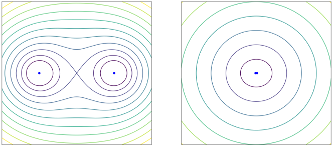
Figure 4.1: Level sets of the function $\rho$ for $M_{+}=M_{-}=1/2$ and $Z=1$ in Cartesian coordinates $(x,y,z)$. The left figure shows the case where $\rho$ is comparable to the value of $Z$. The right figure shows the case $\rho\gg Z$. The blue dots represent the two black hole coordinate positions.

Given the function $\rho$ in Eq. (4.1), we must now make choices for the function $V$ and the tensor $\dot{\gamma}_{ab}$. For $V$ we pick

$$V=1-\frac{27M^{2}}{\rho^{2}},$$ (4.7)

where $M=M_{+}+M_{-}$ is the Bondi mass of the background initial data set in consistency with the spherically symmetric single black hole case in Section 3.2.1. Motivated by the same case (we restrict to $\lambda=0$ in all of what follows), see Eqs. (3.10) and (3.12), we also set

$$\begin{split}\delta\kappa=\frac{\rho(2-V)\eta(\rho\,;M)\partial_{\rho}V+2M(1-V)^{2}+\rho^{2}\partial_{\rho}V}{\rho(1-V)^{2}\eta(\rho\,;M)},\quad\delta q=4\frac{\eta(\rho\,;M)-\rho V}{\rho^{2}(V-1)},\\ \delta Q_{AB}=-\frac{2V}{({1-V})f}(\overset{\star}{k}{}_{AB}-\frac{1}{2}\overset{\star}{k}h_{AB}),\quad\delta p_{A}=0.\end{split}$$ (4.8)

Here $f$, $\overset{\star}{k}_{AB}$ and $\overset{\star}{k}$ are given by the formulas in Section 2.2 and Section 3.1 together with Eqs. (2.10) and (2.11). The particular choice of $\delta Q_{AB}$ here does clearly not agree with Eq. (3.10) except in the single black hole case $M_{-}=0$ or $Z=0$. The rational for this “artificial” choice of $\delta Q_{AB}$ is that it implies that the resulting background tensor field $Q_{AB}$ identically vanishes, while the “more natural” choice $\delta Q_{AB}=0$ would in general violate the divergence condition $D_{A}Q_{BC}(\Omega^{-1})^{AB}=0$ at $\rho=\infty$ of Proposition 3. In any case, we emphasise that in the single black hole case given by $Z=0$ or $M_{-}=0$, this background initial data set reduces to the one considered in Section 3.2.1 (for $\lambda=0$).

We point out here that $M$ is in general not a ‘physical’ mass as our chosen background does not, in general, satisfy the constraints. Only in the special single black hole case $Z=0$ or $M_{-}=0$, the quantity $M$ agrees with Bondi mass.

We also note that with the above choices, $\overset{\star}{k}$ can be shown to satisfy

$$\overset{\star}{k}=-\frac{2}{\rho}+O\left(\frac{1}{\rho^{3}}\right).$$ (4.9)

It is therefore clear that the parabolicity condition Eq. (2.21) holds for all sufficiently large $\rho$. This is consistent with Proposition 3. In numerical calculations we always calculate $\overset{\star}{k}$ in order to verify that the parabolicity condition is satisfied on the whole computational domain. One can also demonstrate that for any $M_{+},M_{-}$ and $Z$ as above, the resulting free data fields $(\kappa,B_{A},h_{AB},h^{AB},Q_{AB})$ satisfy the hypothesis about the free data in Proposition 3 (the hypothesis about the unknown fields $A,q$ and $p_{A}$ can clearly not be verified a-priori). One of the primary goals of the following subsections is to provide numerical evidence that the unknowns $(A,q,p_{A})$ and $p_{A}$ satisfy (at least some of) the a-priori assumptions of Proposition 3. This gives us confidence that the conclusions of Proposition 3, especially that the resulting vacuum initial data sets are asymptotically hyperboloidal and extend smoothly to $t=0$, also hold.

4.2 Numerical implementation

Given a binary black hole background data set as constructed in Section 4.1, the next task is to numerically solve the Cauchy problem of Eqs. (2.16)–(2.18) with free data (and in some cases also the Cauchy data, see below) determined by this background. While the background data sets are given in Cartesian coordinates $(x,y,z)$ on $\Sigma$, or, equivalently, in corresponding spherical coordinates $(r,\theta,\phi)$ using Eq. (4.2), the $2+1$-decomposition underlying Eqs. (2.16)–(2.18) assumes adapted coordinates $(\rho,\vartheta,\varphi)$ where $\rho$ given by Eq. (4.1) labels the leaves of the foliation and $(\vartheta,\varphi)$ are intrinsic polar coordinates on each $\rho=\mathrm{const}$-surface diffeomorphic to $\mathbb{S}^{2}$. As in [18, 19] we choose

$$\vartheta=\theta,\quad\varphi=\phi$$

for simplicity. This together with Eq. (4.1) therefore completely fixes the transformation between the two coordinate systems $(r,\theta,\phi)$ and $(\rho,\vartheta,\varphi)$ on $\Sigma$ and allows us to write the background data sets in Section 4.1 in the required $(\rho,\vartheta,\varphi)$-coordinates. For further details we refer to [18, 19].

Since the computational domain is foliated by $2$-spheres, we can apply the spin-weight formalism following [26, 27, 22, 23, 21, 17]. A brief summary is given in Section A in the appendix. We express the covariant derivative operator $D_{A}$ (defined with respect to the intrinsic metric $h_{AB}$) in terms of the covariant operator $\hat{D}_{A}$ defined with respect to the round unit-sphere metric $\Omega_{AB}$; recall that $D_{A}-\hat{D}_{A}$ can be expressed in terms of smooth intrinsic tensor fields. Using Section A, we can then express the covariant derivative operator $\hat{D}_{A}$ in terms of the $\eth$- and $\eth^{\prime}$-operators. Once all of this has been completed for all terms in Eqs. (2.16)–(2.18), each term of each of these equations ends up with a consistent well-defined spin-weight. Most importantly, however, all terms are explicitly regular: Standard polar coordinate issues at the poles of the $2$-sphere disappear when all quantities are expanded in terms of spin-weighted spherical harmonics and Eqs. (A.5) and (A.6) are used to calculate the intrinsic derivatives. From the numerical point of view this gives rise to a (pseudo)-spectral scheme. We can largely reuse the code presented in [18, 19] subject to three minor changes: (1) the definition of $\rho$ now allows that $Z_{+}\neq Z_{-}$ in agreement with Eq. (4.4), (2) the definition of $V$ is changed agreement with Eq. (4.7), and, (3) the definition of $\dot{\gamma}_{ab}$ is changed in agreement with Eq. (4.8). These three changes do not significantly affect our numerical methods. Once these changes had been made to the code, convergence tests (analogous to the ones presented in [18]) were carried out successfully. All of the following simulations were carried out using the adaptive SciPy ODE solver odeint.

Notice that the background data sets constructed in Section 4.1 are axially symmetric and hence there is no dependence on the angular coordinate $\varphi=\phi$. Motivated by this we restrict to numerical solutions of Eqs. (2.16)–(2.18) with that same symmetry in all of what follows. We can therefore restrict to the axisymmetric case of the spin-weight formalism in Section A.

4.3 Axisymmetric perturbations of single Schwarzschild black hole initial data

In this section now, we use the background data set given in Section 4.1 with the choices $M_{+}=1$, $M_{-}=Z=0$ so that the background initial data set reduces to the spherically symmetric single black case first introduced in Section 3.2.1 with $M=1$ (for $\lambda=0$). This background and therefore the free data for Eqs. (2.16)–(2.18) given by Eq. (3.10) with $V=1-27M^{2}\rho^{-2}$ are therefore spherically symmetric. The fields

$$\mathring{q}=\frac{2\sqrt{3}(1-3\rho^{-1})\sqrt{1+6\rho^{-1}}}{9},\;\;\mathring{A}=\frac{\sqrt{27}}{\rho},\;\;\mathring{p}_{a}=0,$$ (4.10)

agree with the particular solution of Eqs. (2.16)–(2.18) given by Eq. (3.11) (or by Eqs. (3.22) and (3.23) for $\mathcal{C}=0$ and $m=1$) representing single unperturbed spherically symmetric Schwarzschild black hole initial data of unit mass. The purpose of the present subsection is to generate axisymmetric (non-linear) perturbations of this solution by solving Eqs. (2.16)–(2.18) with the same free data, but with the following perturbed Cauchy data imposed at the initial radius $\rho_{0}=5$:

$$\left.q\right|_{\rho=\rho_{0}}=\left.\mathring{q}\right|_{\rho=\rho_{0}}+\epsilon\sin\left(\theta\right),\;\;\left.A\right|_{\rho=\rho_{0}}=\left.\mathring{A}\right|_{\rho=\rho_{0}}+\epsilon\sin\left(\theta\right),\;\;\left.p_{A}\right|_{\rho=\rho_{0}}=0,$$ (4.11)

for some arbitrary constant $\epsilon\in\mathbb{R}$. Especially for small values of $\epsilon$, we can interpret the resulting vacuum initial data sets as (nonlinear) perturbations of single Schwarzschild black hole initial data.

We express Eqs. (2.16)–(2.18) for these free data and Cauchy data numerically in terms of the formalism in Section A:

$$\partial_{\rho}A =-\frac{\rho}{2}\left(\kappa q+\frac{1}{4}q^{2}\right)A^{3}+\frac{1}{2\rho}\left(\left(1+A\eth\left({\eth^{\prime}}\left(A\right)\right)\right)A-\left(1-2p\bar{p}\right)\right),$$ (4.12)

$$\partial_{\rho}q =\frac{1}{\sqrt{2}\rho^{2}}\left({\eth^{\prime}}\left(p\right)+\eth\left(\bar{p}\right)\right)A-\frac{1}{\rho}\left(q-2\kappa\right)+\frac{\sqrt{2}}{\rho^{2}}\left(p{\eth^{\prime}}\left(A\right)+\bar{p}\eth\left(A\right)\right),$$ (4.13)

$$\partial_{\rho}p =\frac{A}{2\sqrt{2}}\eth\left(q\right)-\frac{2}{\rho}p+\frac{1}{\sqrt{2}}\left(\kappa-\frac{1}{2}q\right)\eth\left(A\right),$$ (4.14)

$$\partial_{\rho}\bar{p} =\frac{A}{2\sqrt{2}}{\eth^{\prime}}\left(q\right)-\frac{2}{\rho}\bar{p}+\frac{1}{\sqrt{2}}\left(\kappa-\frac{1}{2}q\right){\eth^{\prime}}\left(A\right),$$ (4.15)

where

$$p=\frac{1}{\sqrt{2}}p_{A}\left(\partial_{\vartheta}^{A}-{\text{i}}\,{\csc\theta}\,\partial_{\varphi}^{A}\right),\quad\bar{p}=\frac{1}{\sqrt{2}}p_{A}\left(\partial_{\vartheta}^{A}+{\text{i}}\,{\csc\theta}\,\partial_{\varphi}^{A}\right),$$ (4.16)

and, see Eq. (3.21) for $M=1$,

$$\kappa=\frac{\rho^{2}+3\rho+9}{\rho^{3/2}\sqrt{27(\rho+6)}}.$$ (4.17)

The quantities $A$ and $q$ have spin-weight zero, while $p$ and $\bar{p}$ have spin-weight $1$ and $-1$, respectively. Our symmetry assumptions (and our particular representation of the bundle of orthonormal frames on $\mathbb{S}^{2}$) allows us to assume that

$$p=\bar{p}.$$

Let us present the numerical results now. To this end we define the $\sup$-norm over $\mathbb{S}^{2}$ for any smooth scalar function $\mathcal{F}(\rho,\vartheta)$ (such as $A$ and $q$ above) as

$$\|\mathcal{F}\|(\rho)=\max_{\vartheta\in[0,\pi]}|\mathcal{F}(\rho,\vartheta)|,$$ (4.18)

while for the covector $p_{A}$, this norm is defined as

$$\|p\|(\rho)=\max_{\vartheta\in[0,\pi]}\sqrt{\left(\Omega^{-1}\right)^{AB}p_{A}(\rho,\vartheta)p_{B}(\rho,\vartheta)}=\max_{\vartheta\in[0,\pi]}\sqrt{p(\rho,\vartheta)\bar{p}(\rho,\vartheta)}.$$ (4.19)

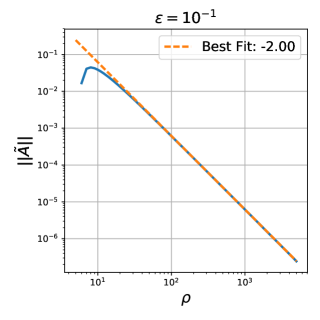
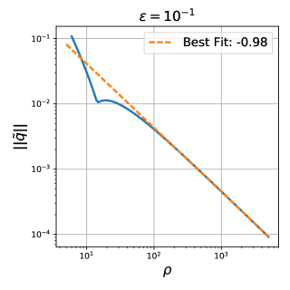
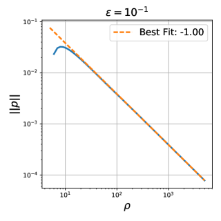
Figure 4.2: The leading order asymptotics for the “single black hole case” obtained with $\epsilon=10^{-1}$, $N=11$ and error tolerance of $10^{-10}$. The definitions of $\tilde{q}$ and $\tilde{A}$ are given in Eq. (4.20). Each numerical curve (solid blue) in the three plots is fitted to the function $C\rho^{k}$ (dashed yellow) for some $C>0$ where “Best fit” gives the best value for $k$.

To discuss the expected behaviour we now introduce the following quantities

$$\tilde{q}=q-\frac{2}{\sqrt{27}M},\quad\tilde{A}=A-\frac{\sqrt{27}M}{\rho}.$$ (4.20)

According to Proposition 2 together with Section 3.1, we expect the following behaviour

$$\left\|\tilde{A}\right\|=O\left(\frac{1}{\rho^{2}}\right),\quad\left\|\tilde{q}\right\|=O\left(\frac{1}{\rho}\right),\quad\|p\|=O\left(\frac{1}{\rho}\right).$$ (4.21)

This is confirmed by the first three plots of Fig. 4.2 for $\epsilon=10^{-1}$, an absolute and relative error tolerance for the adaptive ODE solver of $10^{-10}$, and for $N=11$, where $N$ is the number of spatial points in the $\vartheta$-direction (recall that due to axisymmetry, there is no $\varphi$-dependence). The plots shown in Fig. 4.2 show that our numerically constructed solutions are asymptotic hyperboloidal (at least with minimal regularity at infinity) and are compatible with Proposition 2.

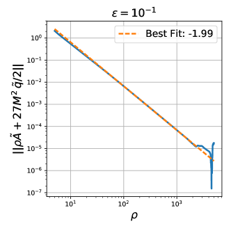
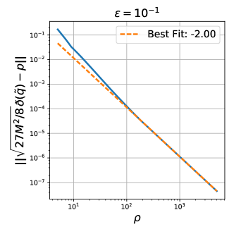
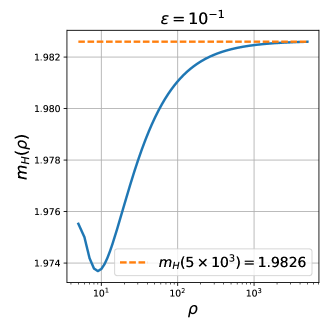
Figure 4.3: Higher order asymptotics and evolution of the Hawking mass $m_{H}$ for the “single black hole case” obtained with the same parameter values as in Fig. 4.2.

Given that our background fields satisfy the assumptions of Proposition 3 we may now wonder to what extent it is possible to also verify the asymptotic expansions Eqs. (3.36)–(3.38) given by that result. To this end we note that Proposition 3 (together with the formulas in Section 2.2) yields that

$$\tilde{q}=\frac{q^{(1)}}{\rho}+O\left(\frac{1}{\rho^{2}}\right),\quad\tilde{A}=-\frac{27M^{2}}{2\rho^{2}}q^{(1)}+O\left(\frac{1}{\rho^{3}}\right),\quad p=\sqrt{\frac{27M^{2}}{8}}\frac{\eth(q^{(1)})}{\rho}+O\left(\frac{1}{\rho^{2}}\right).$$

Combining these, we find that

$$\sqrt{\frac{27M^{2}}{8}}\eth(\tilde{q})-p=O\left(\frac{1}{\rho^{2}}\right),\quad\rho\tilde{A}+\frac{27M^{2}}{2}\tilde{q}=O\left(\frac{1}{\rho^{2}}\right),$$

and hence we have

$$\|\sqrt{27M^{2}/8}\,\eth(\tilde{q})-p\|=O\left(\frac{1}{\rho^{2}}\right),\quad\|\rho\tilde{A}+{27M^{2}}\tilde{q}/2\|=O\left(\frac{1}{\rho^{2}}\right).$$ (4.22)

These theoretically obtained asymptotics are indeed confirmed in the first two plots in Fig. 4.3. Together, Figs. 4.2 and 4.3 verify our theoretical results for $q^{(0)}$, $q^{(1)}$, $A^{(0)}$, $A^{(1)}$, $A^{(2)}$, $p_{B}^{(0)}$ and $p_{B}^{(1)}$. However, the numerical results do not seem to be accurate enough to construct $q^{(2)}$ or $A^{(3)}$.

As mentioned earlier, it turns out that the direct numerical estimation of the Bondi mass via Eqs. (3.31) and (3.32) is unsuccessful. The limit appears to diverge as a consequence of numerical errors. This is why we determine Bondi mass by evolving the quantity $m_{H}$ by means of Eqs. (3.48) and (3.46) simultaneously with Eqs. (4.12)–(4.15). Since the background initial data set is spherically symmetric, so in particular $\overset{\star}{k}=-2/\rho$, the evolution equation for $m_{H}$ takes the form here

$$\partial_{\rho}m_{H}=\frac{\rho^{2}}{8}\underline{F_{[a]}},$$ (4.23)

where we use $\overset{\star}{k}=-2/\rho$, $t=1/\rho$, Eq. (A.8), and

$$\begin{split}\underline{F_{[a]}}=\int_{d\Omega}{\frac{8}{\rho^{2}}p\bar{p}}+{\sqrt{2}}q^{2}\left(\bar{p}\,\eth\left(\frac{A}{q}\right)+{p}\,\eth^{\prime}\left(\frac{A}{q}\right)\right)\rho-\frac{4}{\rho^{2}}A^{-2}\eth(A){\eth^{\prime}}(A)\,d\Omega.\end{split}$$ (4.24)

The numerically calculated function $m_{H}(\rho)$ is shown in the last plot of Fig. 4.3. Here we see that it quickly converges to a constant number approximating the Bondi mass $m$ as $m=m_{H}(\rho)$ for $\rho=5\times 10^{3}$. It is of course natural to wonder how good this approximation is. For this we consider the quantity

$$\mathcal{E}_{A}[m]=|m_{H}(2\rho)-m_{H}(\rho)|,$$ (4.25)

which is calculated for $\rho=5\times 10^{3}$, as an approximation of the absolute (and approximately also relative) error. For our example case with $\epsilon=10^{-1}$ we find

$$m=1.9826,\quad\mathcal{E}_{A}[m]=1.654\times 10^{-6}.$$ (4.26)

Notice that the main error source here is likely the error associated with measuring $m$ at a finite value of $\rho$. However, due to the errors generated by numerically solving the constraints for very large values of $\rho$, we find that evaluating the mass at $\rho=5\times 10^{3}$ is optimal. Indeed, in the first plot of Fig. 4.3 we see that the numerical errors become important at around $\rho\sim 10^{3}$.

4.4 Binary black hole-like initial data sets

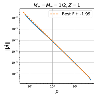
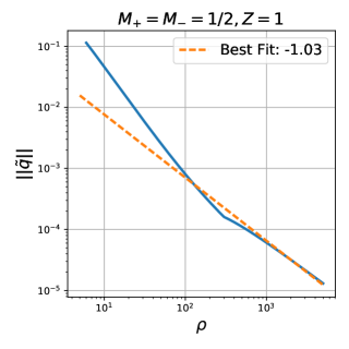
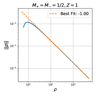
Figure 4.4: The leading order asymptotics for the “binary black hole case” obtained with $M_{+}=M_{-}=1/2$, $\rho_{0}=3$, $N=11$ and numerical error tolerance of $10^{-10}$. Each numerical curve (solid blue) in the three plots is fitted to the function $C\rho^{k}$ (dashed yellow) for some $C>0$ where “Best fit” gives the best value for $k$.

In this subsection we essentially repeat the same numerical experiments as before with two changes: (1), the background initial data set is now determined with parameters $M_{+}=M_{-}=1/2$ and $Z=1$ (an “equal mass binary black hole case”), and (2), instead of the “perturbed” Cauchy data as in Eq. (4.11), we now choose the values obtained from the background data set at $\rho_{0}=5$. For this particular case Eq. (4.6) gives $\rho_{crit}=1$. Our numerical findings, as shown in the first three plots of Fig. 4.4 are again consistent with Eq. (4.21) as expected from Proposition 2. Similarly, the first two plots of Fig. 4.5 are consistent with Eq. (4.22) and therefore, as with the “single black hole case”, support Proposition 3. We interpret this as strong evidence that the vacuum initial data sets we have numerically calculated are asymptotically hyperboloidal.

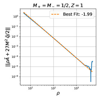
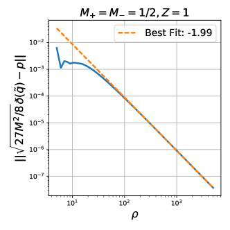
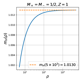
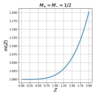
Figure 4.5: Higher order asymptotics and evolution of the Hawking mass $m_{H}$ for the “binary black hole case” obtained with the same parameter values as in Fig. 4.4.

Constructing the Bondi mass in the same way as in Section 4.3 yields the third plot in Fig. 4.5, and

$$m=1.01297,\quad\mathcal{E}_{A}[m]=3.78\times 10^{-6}.$$ (4.27)

For fixed values of $M_{+}$ and $M_{-}$, say, $M_{+}=M_{-}=1/2$ as before, one expects the resulting Bondi masses to depend strongly on the separation parameter $Z$. To investigate this we numerically calculate the resulting vacuum initial data sets and Bondi masses for a range of separation parameter values $Z$. Since we treat $\rho_{0}=5$ as fixed, Eq. (4.6) introduces an upper bound for the possible values for $Z$, namely $Z<\rho_{0}$. The results of our numerical calculations are shown in the last plot of Fig. 4.5. Observe that the Bondi mass turns out to be an increasing function of $Z$. For $Z=0$ (in which the single black hole solution is obtained) we find that $m=1$, as expected. Observe that the case $Z=0$ here is different from the single black hole case in Section 4.3 because the Cauchy data are determined differently. When $Z$ is now increased we find that the Bondi mass becomes larger. This is intuitive as one expects the (negative) gravitational binding energy to become small as the separation distance $Z$ is increased. However, it is interesting to compare this to our results in [18, 19] for asymptotically flat initial data sets, where we found that the ADM mass decreases as a function of the separation distance $Z$.

5 Conclusions

In this paper we discuss the asymptotic behaviour of vacuum initial data sets constructed as solutions of a parabolic-hyperbolic formulation of the vacuum constraint equations. The primary goal of this work is to establish whether or not it is possible to reliably construct asymptotically hyperboloidal initial data sets using Rácz’s parabolic-hyperbolic formalism.

We found that initial data sets constructed as solutions of Rácz’s original parabolic-hyperbolic formulation of the constraints on asymptotically hyperboloidal background initial data sets are, in general, asymptotically hyperboloidal with a well-defined Bondi mass. In particular, no modifications are necessary (in contrast to the asympotically flat case) as long as the background initial data set used to construct the free data for the equations satisfy certain properties at $\rho=\infty$. In fact we provide explicit conditions together with strong evidence guaranteeing that $\log\rho$-terms in expansions at $\rho=\infty$ are completely ruled out and the resulting vacuum initial data sets therefore extend to infinity smoothly. This contrasts the more traditional conformal approach where it was found [28] that asymptotically hyperboloidal initial data sets are in general poly-logarithmic at infinity unless the condition $K=const$ in [28] holds.

Appendix A Spin-weight and spin-weighted spherical harmonics

We say that a function $f$ defined on $\mathbb{S}^{2}$ has spin-weight $s$ if it transforms as $f\to e^{\text{i}s\xi}f$ under a local rotation by an angle $\xi$ in the tangent plane at any point in $\mathbb{S}^{2}$. Let $(\vartheta,\varphi)$ be standard polar coordinates on $\mathbb{S}^{2}$. If $f$ has spin-weight $s$ and is sufficiently smooth, it can be written as

$$f(\vartheta,\varphi)=\sum\limits_{l=|s|}^{\infty}\sum\limits_{m=-l}^{l}f_{lm}\,{}_{s}Y_{lm}(\vartheta,\varphi),$$ (A.1)

where ${}_{s}Y_{lm}(\vartheta,\varphi)$ are the spin-weighted spherical harmonics (SWSH) and where $f_{lm}$ are complex numbers. Using the conventions in [26, 27, 22, 23, 21, 17], these functions satisfy

$$\int\limits_{\mathbb{S}^{2}}\ {}_{s}Y_{l_{1}m_{1}}(\vartheta,\varphi)\>_{s}\overline{Y}_{l_{2}m_{2}}(\vartheta,\varphi)\ d\Omega=\delta_{l_{1}l_{2}}\delta_{m_{1}m_{2}},$$ (A.2)

where $\delta_{lm}$ is the Kronecker delta and $d\Omega$ is the area element of the metric of the round unit sphere. Using this we find that the coefficients $f_{lm}$ in Eq. (A.1) can be calculated as

$$f_{lm}=\int\limits_{\mathbb{S}^{2}}f(\vartheta,\varphi)\,{}_{s}\overline{Y}_{lm}(\vartheta,\varphi)d\Omega.$$ (A.3)

The eth-operators $\eth$ and $\eth^{\prime}$ are defined by

$$\eth f=\partial_{\vartheta}f-\dfrac{\text{i}}{\sin\vartheta}\partial_{\varphi}f-sf\cot\vartheta,\quad\eth^{\prime}f=\partial_{\vartheta}f+\dfrac{\text{i}}{\sin\vartheta}\partial_{\varphi}f+sf\cot\vartheta,$$ (A.4)

for any function $f$ on $\mathbb{S}^{2}$ with spin-weight $s$. We have

$$\eth\hskip 2.84544pt_{s}Y_{lm}(\vartheta,\varphi) =-\sqrt{(l-s)(l+s+1)}\hskip 2.84544pt_{s+1}Y_{lm}(\vartheta,\varphi),$$ (A.5)

$$\eth^{\prime}\hskip 2.84544pt_{s}Y_{lm}(\vartheta,\varphi) =\sqrt{(l+s)(l-s+1)}\hskip 2.84544pt_{s-1}Y_{lm}(\vartheta,\varphi),$$ (A.6)

$$\eth^{\prime}\eth\hskip 2.84544pt_{s}Y_{lm}(\vartheta,\varphi) =-(l-s)(l+s+1)\hskip 2.84544pt_{s}Y_{lm}(\vartheta,\varphi).$$ (A.7)

Thus, using the properties above it is easy to see that $\eth$ raises the spin-weight by one while $\eth^{\prime}$ lowers it by one.

In our discussion we are often interested in the average of a function $f$ with spin-weight $0$ on $\mathbb{S}^{2}$ defined by

$$\underline{f}=\dfrac{1}{4\pi}\int\limits_{\mathbb{S}^{2}}\>fd\Omega.$$ (A.8)

Expressing $f$ in terms of SWSH and using Eq. (A.2) it follows

$$\underline{f} =\dfrac{1}{4\pi}\int\limits_{\mathbb{S}^{2}}\>\sum\limits_{l=0}^{\infty}\sum\limits_{m=-l}^{l}f_{lm}\,{}_{0}Y_{lm}(\vartheta,\varphi)\;d\Omega,$$ (A.9)

$$=\dfrac{\sqrt{4\pi}}{4\pi}\int\limits_{\mathbb{S}^{2}}\>\sum\limits_{l=0}^{\infty}\sum\limits_{m=-l}^{l}f_{lm}\,{}_{0}Y_{lm}(\vartheta,\varphi)\;_{0}\overline{Y}_{00}(\vartheta,\varphi)\;d\Omega,$$

$$=\frac{1}{\sqrt{4\pi}}f_{00},$$

where we have used the fact that ${}_{0}Y_{00}(\vartheta,\varphi)=(4\pi)^{-1/2}$. Another quantity of interest is the $L^{2}$-norm with respect to the standard round metric on $S^{2}$. The Parseval identity states that

$$\|f\|^{2}_{L^{2}(\mathbb{S}^{2})}=\sum_{l=0}^{\infty}\sum_{m=-l}^{l}|f_{lm}|^{2}.$$ (A.10)

Finally we notice that all functions considered in this paper are axially symmetric and therefore do not depend on the angle $\varphi$. For such functions, all coefficients with $f_{lm}$ with $m\not=0$ vanish and we use the following short-hand notation to write Eq. (A.1) as

$$f(\vartheta)=\sum\limits_{l=|s|}^{\infty}f_{l}\,{}_{s}Y_{l}(\vartheta).$$ (A.11)

Appendix B Asymptotically hyperbolodial initial data sets from other evolutionary formulations of the constraints

Although this paper focuses on Rácz’s “original” parabolic-hyperbolic system Eqs. (2.16)–(2.18), we would also like present some brief results about other evolutionary formulations of the constraints. The goal of this Appendix here is to introduce and discuss two other evolutionary formulations of the constraints.

B.1 Other evolutionary formulations of the constraints

B.1.1 A modified parabolic-hyperbolic formulation of the constraints

We start with our “modified” parabolic-hyperbolic formulation of the vacuum constraints which was first presented by us in [19] when considering asymptotically flat initial data sets.

First, recall that $\kappa$ is one of the free data in the formulation introduced in Section 2.1 while $q$ is one of the unknowns. We modify Eqs. (2.16)–(2.18) by introducing a new free data field $\mathcal{R}$ such that

$$\kappa=\mathcal{R}q$$ (B.1)

where $q$ continues to be an unknown. The equations obtained from Eqs. (2.16)–(2.18) by replacing all instances of $\kappa$ with $\mathcal{R}q$ are

$$\overset{\star}{k}\mathcal{L}_{\rho}A+A^{2}D^{C}D_{C}A-\overset{\star}{k}B^{C}D_{C}A=\, \frac{1}{2}A^{3}E+\frac{1}{2}AF,$$ (B.2)

$$\mathcal{L}_{\rho}q-B^{C}D_{C}q-AD_{C}p^{C}-2p^{C}D_{C}A=\, \overset{\star}{k}{}^{CS}Q_{CS}+\frac{1}{2}q\overset{\star}{k}-\overset{\star}{k}\mathcal{R}q,$$ (B.3)

$$\begin{split}\mathcal{L}_{\rho}p_{C}-B^{S}D_{S}p_{C}-A\left(\frac{1}{2}+\mathcal{R}\right)D_{C}q=\,&p_{S}D_{C}B^{S}-AD_{S}{Q^{S}}_{C}+q\mathcal{R}D_{C}A-{Q^{S}}_{C}D_{S}A\\ &+\overset{\star}{k}p_{C}+AqD_{C}\mathcal{R}-\frac{1}{2}qD_{C}A,\end{split}$$ (B.4)

where, $F$ takes the same form as in Eq. (2.20) and $E$ becomes

$$E ={}^{(2)}R-2p^{C}p_{C}-Q_{CS}Q^{CS}+\left(2\mathcal{R}+\frac{1}{2}\right)q^{2}.$$ (B.5)

We refer to these equations as the modified parabolic-hyperbolic system while Eqs. (2.16)–(2.18) is often labelled as the original parabolic-hyperbolic system.

While Eq. (B.1) looks like a minor modification, it has dramatic consequences for the asymptotics of the solutions [19] because of the different way the free data for these equations are specified, see below. First observe that this modification has changed some of the principal part of the system. While the principal part of Eq. (B.2) is unchanged (and is therefore parabolic provided Eq. (2.21) holds as before), the subsystem Eqs. (B.3) – (B.4) turns out to be symmetrisable hyperbolic with symmetriser

$$\left(\begin{array}[]{cc}\frac{1}{2}+\mathcal{R}&0\\ 0&h^{AB}\end{array}\right)$$ (B.8)

provided

$$\frac{1}{2}+\mathcal{R}>0,$$ (B.9)

where $h^{AB}$ is the intrinsic inverse of $h_{AB}$. We refer to Eq. (B.9) as the hyperbolicity condition. It therefore turns out that Eqs. (B.2)–(B.4) is parabolic-hyperbolic provided Eqs. (2.21) and (B.9) hold.

The structure of these equations suggest to group the various fields as follows:

Free data:

The fields $B_{A}$, $Q_{AB}$, $h_{AB}$ and $\mathcal{R}$ are free data everywhere on $\Sigma$.

Unknowns:

The fields $A$, $q$ and $p_{A}$ are the unknowns.

Cauchy data:

The initial values of the fields $A,q$ and $p_{C}$ on some $\rho=\rho_{0}$-surface is the Cauchy data.

It is important to notice that similar to Rácz’s “original” parabolic-hyperbolic system Eqs. (2.16)–(2.18), the PDE conditions Eqs. (2.21) and (B.9) are properties of the free data alone and can therefore be verified before solutions are constructed. In particular, if these conditions for the free data are met, the Cauchy problem in the increasing $\rho$-direction is well-posed. We briefly comment on the claim in [20] that it is sufficient to interpret our modified formulation Eqs. (B.2)–(B.4) of the vacuum constraints (introduced in [19]) as the special case of Rácz’s “original” formulation Eqs. (2.16)–(2.18) where the free field $\kappa$ is chosen to be determined by Eq. (B.1) in terms of some given field $\mathcal{R}$ and the unknown $q$ “on the fly” at each time step of the evolution; see Section 4.3.1 in [20]. While this claim is evident on the one hand (because both the modified and the original formulations represent the same Einstein vacuum constraints), it may also be misleading. The reason is that this point of view neglects the significant role played by the new hyperbolicity condition Eq. (B.9) implied by the new principal part of the resulting PDEs. Indeed it is possible to construct numerical examples which do not converge when Eq. (B.9) is violated.

B.1.2 An algebraic-hyperbolic formulation of the constraints

We end this subsection by discussing Rácz’s algebraic-hyperbolic formulation of the constraints [13]. Based on the same $2+1$-framework discussed in Section 2.1, we now write the Hamiltonian constraint as the following algebraic equation to determine the quantity $\kappa$

$$\kappa=\frac{1}{2q}\left(-^{(3)}R+Q^{AB}Q_{AB}-\frac{1}{2}q^{2}+2p_{C}p^{C}\right),$$ (B.10)

instead of as the PDE (2.16) to determine $A$. To this end we consider $A$ as a free field now (as opposed to the unknown in Rácz’s parabolic-hyperbolic formulation), while $\kappa$ is now determined algebraically from the other fields by Eq. (B.10) (and is therefore not anymore interpreted as the free field of Rácz’s parabolic-hyperbolic formulation). The equations resulting from this are

$$\begin{split}\mathcal{L}_{\rho}p_{C}-B^{A}D_{A}p_{C}&+\frac{A\kappa}{q}D_{C}q-\frac{2A}{q}p_{A}D_{C}p^{A}=\,p_{A}D_{B}B^{A}+\overset{\star}{k}p_{C}+\kappa D_{C}A\\ &-{Q^{A}}_{C}D_{A}A-\frac{1}{2}qD_{C}A-AD_{A}{Q^{A}}_{C}+\frac{A}{2q}D_{C}(-^{(3)}R+Q_{AB}Q^{AB}),\end{split}$$ (B.11)

$$\mathcal{L}_{\rho}q-B^{A}D_{A}q-AD_{A}p^{A}=\overset{\star}{k}{}^{AB}Q_{AB}+\frac{1}{2}q\overset{\star}{k}-\overset{\star}{k}\kappa+2p_{C}D^{C}A,$$ (B.12)

where $\prescript{(3)}{}{R}$ is given by Eq. (2.12) and $\kappa$ by Eq. (B.10). We refer to this as the algebraic-hyperbolic formulation of the Einstein vacuum constraints.

According to [11], the system Eqs. (B.10)–(B.12) is symmetrisable hyperbolic with symmetriser

$$\left(\begin{array}[]{cc}-\frac{\kappa}{q}&0\\ 0&h^{AB}\end{array}\right)$$ (B.15)

provided

$$\kappa q<0.$$ (B.16)

We refer to Eq. (B.16) as the algebraic-hyperbolicity condition. This should not be confused with the hyperbolicity condition Eq. (B.9) associated with our modified parabolic-hyperbolic system in Section B.1.1.

All of this suggests to group the $(2+1)$-fields in the following way for this formulation:

Free data:

The fields $B_{A}$, $Q_{AB}$, $h_{AB}$ and $A$ are the free data everywhere on $\Sigma$.

Unknowns:

The quantities $q$ and $p_{A}$ are considered as the unknowns.

Cauchy data:

The initial values of the fields $q$ and $p_{A}$ on some $\rho=\rho_{0}$-surface is the Cauchy data.

It follows that for arbitrary free data and Cauchy data, for which the algebraic-hyperbolicity condition Eq. (B.16) holds on the initial leaf $\rho=\rho_{0}$, Eqs. (B.10)–(B.12) is a hyperbolic system, and, the Cauchy problem (in both the increasing and decreasing $\rho$-directions) is well-posed. Note, however that the algebraic-hyperbolicity condition Eq. (B.16) is not just a property of the free data. Due to its depends on the unknowns, it is possible to fail during the evolution even if it holds initially.

B.2 Remarks about other evolutionary formulations of the constraints

Given the results of Sections 3.2.1 and 3.2.2 it is natural to wonder whether or not is possible to construct asymptotically hyperboloidal initial data sets using the other evolutionary formulations of the constraints (discussed in Section B.1). This is exactly the issue that we address in the present subsection. In particular, we provide some evidence that the two evolutionary formulations presented in Section B.1 are not well suited to the construction of asymptotically hyperboloidal initial data sets.

B.2.1 Algebraic-hyperbolic formulation

We first discuss the algebraic-hyperbolic formulation, introduced in Section B.1.2. Suppose that we had constructed a solution of the algebraic-hyperbolic constraints Eqs. (B.10)–(B.12) that is asymptotically hyperboloidal in accordance with Proposition 1. As a consequence we would have

$$\kappa q=2\left(\kappa^{(0)}\right)^{2}+O\left(\frac{1}{\rho}\right).$$ (B.17)

It is clear then that the condition (B.16) $\kappa q<0$ would be violated for all sufficiently large $\rho$. In particular, we conclude that the algebraic-hyperbolic formulation does not have a well-posed Cauchy problem near $\rho=\infty$ in the asymptotically hyperboloidal setting. This is consistent with the findings in [30]. We shall therefore not discuss this formulation any further.

B.2.2 Modified parabolic-hyperbolic formulation

Let us now consider the modified parabolic-hyperbolic formulation presented in Section B.1.1. According to [19] the fields

$$\mathcal{R}=\frac{(2-V)\rho}{4\left(1-V\right)}\frac{\partial_{\rho}V}{V},\quad\quad B_{A}=0,\quad Q_{AB}=0,\quad h_{AB}=\rho^{2}\Omega_{AB}$$ (B.18)

and

$$q=\frac{2\mathcal{C}\,V}{\rho\sqrt{1-V}},\quad A=\sqrt{\frac{(1-V)\rho}{\rho-2m-(\rho-2m)V+\rho\,\mathcal{C}^{2}V^{2}}},\quad p_{A}=0,$$ (B.19)

constitute a spherically symmetric solution of the modified parabolic-hyperbolic system Eqs. (B.2)–(B.4), where $\mathcal{C}$ is a free constant and $m$ is the mass.

Suppose now that we set $V=1-\mathcal{V}/\rho^{2}$, for some constant $\mathcal{V}>0$. Then, the solutions Eq. (B.19) have asymptotic radial expansions

$$\begin{split}A=\frac{\sqrt{\mathcal{V}}}{|\mathcal{C}|\rho}+O\left(\frac{1}{\rho^{3}}\right),\quad q=\frac{\mathcal{C}}{\sqrt{\mathcal{V}}}-\frac{\sqrt{\mathcal{V}}\mathcal{C}}{\rho^{2}},\quad\kappa=\mathcal{R}q=\frac{\mathcal{C}}{2\sqrt{\mathcal{V}}}+\frac{\mathcal{C}\sqrt{\mathcal{V}}}{2\rho^{2}},\end{split}$$ (B.20)

and Eq. (B.18) gives

$$\mathcal{R}=\frac{\rho^{2}+\mathcal{V}}{2\rho^{2}-2\mathcal{V}}\implies\frac{1}{2}+\mathcal{R}=\frac{\rho^{2}}{\rho^{2}-\mathcal{V}}.$$ (B.21)

It is a consequence of Proposition 1 the associated initial data set is therefore asymptotically hyperboloidal.

An interesting particular solution is now obtained by setting the Cauchy data equal to the values of the background data set at $\rho=\rho_{0}$. A straightforward calculation shows that the parameter values $\mathcal{C}$ and $m$ corresponding to this particular solution of the vacuum constraints are

$$\mathcal{C}=1,\quad m=\frac{1}{2}\left(\frac{\mathcal{V}-\rho_{0}^{2}}{\rho_{0}}\right).$$ (B.22)

We conclude that if the vacuum initial data set resulting from this is supposed to have a non-negative Bondi mass, we must pick $\mathcal{V}-\rho_{0}^{2}\geq 0$. However, if this is true then, from Eq. (B.21), we get $1/2+\mathcal{R}<0$ (at $\rho=\rho_{0}$) and hence we conclude that the hyperbolicity condition Eq. (B.9) is violated. Again we conclude that the modified parabolic-hyperbolic formulation does in general not have well-posed Cauchy problem in the asymptotically hyperboloidal setting. For this reason, we shall not discuss this formulation any further here.

References

- [1] Yvonne Fourès-Bruhat. Théorème d’existence pour certains systèmes d’équations aux dérivées partielles non linéaires. Acta Math., 88(1):141–225, 1952. DOI: 10.1007/BF02392131.
- [2] Yvonne Choquet-Bruhat and Robert P Geroch. Global aspects of the Cauchy problem in general relativity. Commun. Math. Phys., 14(4):329–335, 1969. DOI: 10.1007/BF01645389.
- [3] Robert A Bartnik and James Isenberg. The Constraint Equations. In The Einstein Equations and the Large Scale Behavior of Gravitational Fields, pages 1–38. Birkhäuser Physics, 2004.
- [4] Thomas W Baumgarte and Stuart L Shapiro. Numerical Relativity. Solving Einstein’s Equations on the Computer. Cambridge University Press, 2010.
- [5] James Dilts, Michael Holst, Tamara Kozareva, and David Maxwell. Numerical Bifurcation Analysis of the Conformal Method. 2017. Preprint. arXiv:1710.03201.
- [6] Michael T. Anderson. On the conformal method for the Einstein constraint equations. 2018. Preprint. arXiv:1812.06320.
- [7] Nigel T Bishop, Richard Isaacson, Manoj Maharaj, and Jeffrey Winicour. Black hole data via a Kerr-Schild approach. Phys. Rev. D, 57(10):6113–6118, 1998. DOI: 10.1103/PhysRevD.57.6113.
- [8] Richard A Matzner, Mijan F Huq, and Deirdre Shoemaker. Initial data and coordinates for multiple black hole systems. Phys. Rev. D, 59(2):024015, 1998. DOI: 10.1103/PhysRevD.59.024015.
- [9] Claudia Moreno, Darío Núñez, and Olivier Sarbach. Kerr–Schild-type initial data for black holes with angular momenta. Class. Quantum Grav., 19(23):6059–6073, 2002. DOI: 10.1088/0264-9381/19/23/312.
- [10] Nigel T Bishop, Florian Beyer, and Michael Koppitz. Black hole initial data from a nonconformal decomposition. Phys. Rev. D, 69(6):325, 2004. DOI: 10.1103/PhysRevD.69.064010.
- [11] István Rácz. Cauchy problem as a two-surface based ‘geometrodynamics’. Class. Quantum Grav., 32(1):015006, 2015. DOI: 10.1088/0264-9381/32/1/015006.
- [12] István Rácz. Is the Bianchi identity always hyperbolic? Class. Quantum Grav., 31(15):155004, 2014. DOI: 10.1088/0264-9381/31/15/155004.
- [13] István Rácz. Constraints as evolutionary systems. Class. Quantum Grav., 33(1):015014, 2016. DOI: 10.1088/0264-9381/33/1/015014.
- [14] István Rácz and Jeffrey Winicour. Black hole initial data without elliptic equations. Phys. Rev. D, 91(12):124013, 2015. DOI: 10.1103/PhysRevD.91.124013.
- [15] László B Szabados. Quasi-Local Energy-Momentum and Angular Momentum in General Relativity. Living Rev. Relativity, 12(4):76, 2009. DOI: 10.1088/0264-9381/14/1a/016.
- [16] Carla Cederbaum, Julien Cortier, and Anna Sakovich. On the center of mass of asymptotically hyperbolic initial data sets. Annales Henri Poincaré, 17(6):1504–1528, 2016. DOI: 10.1007/s00023-015-0438-5.
- [17] Florian Beyer, Leon Escobar, and Jörg Frauendiener. Asymptotics of solutions of a hyperbolic formulation of the constraint equations. Class. Quantum Grav., 34(20):205014, 2017. DOI: 10.1088/1361-6382/aa8be6.
- [18] Florian Beyer, Leon Escobar, Jörg Frauendiener, and Joshua Ritchie. Numerical construction of initial data sets of binary black hole type using a parabolic-hyperbolic formulation of the vacuum constraint equations. Class. Quantum Grav., 36(17):175005, 2019. DOI: 10.1088/1361-6382/ab3482.
- [19] Jörg Frauendiener Florian Beyer and Joshua Ritchie. Asymptotically flat vacuum initial data sets from a modified parabolic-hyperbolic formulation of the Einstein vacuum constraint equations. Phys. Rev. D, 101:084013, Apr 2020. DOI: 10.1103/PhysRevD.101.084013.
- [20] Károly Csukás and István Rácz. Numerical investigations of the asymptotics of solutions to the evolutionary form of the constraints. Class. Quantum Grav., 37(15):155006, 2020. DOI: 10.1088/1361-6382/ab8fce.
- [21] Florian Beyer, Leon Escobar, and Jörg Frauendiener. Criticality of inhomogeneous Nariai-like cosmological models. Phys. Rev. D, 95(8):084030, 2017. DOI: 10.1103/PhysRevD.95.084030.
- [22] Florian Beyer, Boris Daszuta, Jörg Frauendiener, and Ben Whale. Numerical evolutions of fields on the 2-sphere using a spectral method based on spin-weighted spherical harmonics. Class. Quantum Grav., 31(7):075019, 2014. DOI: 10.1088/0264-9381/31/7/075019.
- [23] Florian Beyer, Leon Escobar, and Jörg Frauendiener. Numerical solutions of Einstein’s equations for cosmological spacetimes with spatial topology and symmetry group . Phys. Rev. D, 93(4):043009, 2016. DOI: 10.1103/PhysRevD.93.043009.
- [24] Florian Beyer. A spectral solver for evolution problems with spatial -topology. J. Comp. Phys., 228(17):6496–6513, 2009. DOI: 10.1016/j.jcp.2009.05.037.
- [25] Miguel Alcubierre. Introduction to 3+1 Numerical Relativity. Oxford Science Publications, 2008.
- [26] Roger Penrose and Wolfgang Rindler. Two-Spinor Calculus and Relativistic Fields, volume 1 of Spinors and Space-Time. Cambridge University Press, Cambridge, 1984.
- [27] Florian Beyer, Boris Daszuta, and Jörg Frauendiener. A spectral method for half-integer spin fields based on spin-weighted spherical harmonics. Class. Quantum Grav., 32(17):175013, 2015. DOI: 10.1088/0264-9381/32/17/175013.
- [28] Lars Andersson and Piotr T. Chruściel. Solutions of the constraint equations in general relativity satisfying “hyperboloidal boundary conditions”. Department of Mathematics, Royal Institute of Technology, S10044 Stockholm, Sweden, 1996. URL: homepage.univie.ac.at.
- [29] Roger Penrose and Wolfgang Rindler. Spinor and Twistor Methods in Space-Time Geometry, volume 2 of Spinors and Space-Time. Cambridge University Press, 1986.
- [30] Joshua Ritchie. Asymptotics of solutions in evolutionary formulations of the Einstein constraint equations. Master’s thesis, University of Otago, Febuary 2018.