A norm minimization-based convex vector optimization algorithm

Abstract

We propose an algorithm to generate inner and outer polyhedral approximations to the upper image of a bounded convex vector optimization problem. It is an outer approximation algorithm and is based on solving norm-minimizing scalarizations. Unlike Pascolleti-Serafini scalarization used in the literature for similar purposes, it does not involve a direction parameter. Therefore, the algorithm is free of direction-biasedness. We also propose a modification of the algorithm by introducing a suitable compact subset of the upper image, which helps in proving for the first time the finiteness of an algorithm for convex vector optimization. The computational performance of the algorithms is illustrated using some of the benchmark test problems, which shows promising results in comparison to a similar algorithm that is based on Pascoletti-Serafini scalarization.

Keywords and phrases: convex vector optimization, multiobjective optimization, approximation algorithm, scalarization, norm minimization.

Mathematics Subject Classification (2020): 90B50, 90C25, 90C29.

1 Introduction

In multiobjective optimization, the decision-maker is supposed to consider multiple objective functions simultaneously. In general, these functions conflict in the sense that improving one objective leads to deteriorating some of the others. Consequently, there does not exist a feasible solution which can generate optimal values of all the objectives. Rather, there exists a subset of feasible solutions, called efficient solutions, which map to the so called nondominated points in the objective space. The image of a feasible solution is said to be nondominated if none of the objective functions can be improved in value without degrading some of the other objective values.

In vector optimization, the objective function takes values again in a vector space, namely, the objective space. However, rather than comparing the objective function values componentwise as in the multiobjective case, a more general order relation, which is induced by an ordering cone, is used for this purpose. Clearly, multiobjective optimization can be seen as a special case where the ordering cone is the positive orthant. Assuming that the vector optimization problem (VOP) is a minimization problem with respect to an ordering cone $C$, the concept of nondominated point for a multiobjective optimization problem (MOP) is generalized to minimal point with respect to $C$ in the vector optimization case.

A special class of vector optimization problems is the linear VOPs, where the objective function is linear and the feasible region is a polyhedron. There is rich literature available discussing various methods and algorithms for solving linear VOPs. They deal with the problem by generating either the efficient solutions in the decision space [16, 41] or the nondominated points in the objective space [4, 28, 32]. The reader is referred to the books by Ehrgott [14] and by Jahn [23] for the details of these approaches.

In 1998, Benson proposed an outer approximation algorithm for linear MOPs which generates the set of all nondominated points in the objective space rather than the set of all efficient points in the decision space [4]. Later, this algorithm is extended to solve linear VOPs, see [28]. The main principle of the algorithm is that if one adds the ordering cone to the image of the feasible set, then the resulting set, called the upper image, contains all nondominated points in its boundary. The algorithm starts with a set containing the upper image and iterates by updating the outer approximating set until it is equal to the upper image.

For nonlinear MOPs/VOPs, there is a further subdivision, namely the convex and the nonconvex problems. Note that the methods described for linear MOPs/VOPs may not be directly applicable to these classes as, in general, it is not possible to generate the set of all nondominated/minimal points in the objective space. Therefore, approximation algorithms, which approximate the set of all minimal points in the objective space, are widely explored in the literature, refer for example to the survey paper by Ruzika and Wiecek [42] for the multiobjective case.

For bounded convex vector optimization problems (CVOPs), see Section 3 for precise definitions, there are several outer approximation algorithms in the literature that work on the objective space. In [13], the algorithm in [4] is extended for the case of convex MOPs. Another extension of Benson’s algorithm for the vector optimization case is proposed in [29], which is a simplification and generalization of the algorithm in [13]. This algorithm has already been used for solving mixed-integer convex multiobjective optimization problems [10], as well as problems in stochastic optimization [2] and finance [18, 40]. Recently, in [11], a modification of the algorithm in [29] is proposed. The main idea of these algorithms is to generate a sequence of better approximating polyhedral supersets of the upper image until the approximation is sufficiently fine. This is done by sequentially solving some scalarization models in which the original CVOP is converted into an optimization problem with a single objective. There are many scalarization methods available in the literature for MOPs/VOPs, see for instance the book by Eichfelder [15] as well as the recent papers [7, 24, 27].

In particular, in each iteration of the CVOP algorithms proposed in [11, 13, 29], a Pascoletti-Serafini scalarization [38], which requires a reference point $v$ and a direction vector $d$ in the objective space as its parameters, is solved. For the algorithms in [13] and [29], the reference point $v$ is selected to be an arbitrary vertex of the current outer approximation of the upper image. Moreover, in [13], the direction parameter $d$ is computed depending on the reference point $v$ together with a fixed point in the objective space, whereas it is fixed throughout the algorithm proposed in [29]. In [11], a procedure to select a vertex $v$ as well as a direction parameter $d$, which depends on $v$ and the current approximation, is proposed.

In this study, we propose an outer approximation algorithm (Algorithm 1) for CVOPs, which solves a norm-minimizing scalarization in each iteration. Different from Pascoletti-Serafini scalarization, it does not require a direction parameter; hence, one does not need to fix a direction parameter as in [29], or a point in the objective space in order to compute the direction parameter as in [13]. Moreover, when terminates, the algorithm provides the Hausdorff distance between the upper image and its outer approximation, directly.

The scalarization methods based on a norm have been frequently used in the context of MOPs, see for instance [15]. These methods generally depend on the ideal point at which all objectives of the MOP attain its optimal value, simultaneously. Since the ideal point is not feasible in general, the idea is to find the minimum distance from the ideal point to the image of the feasible region. One of the well-known methods is the weighted compromise programming problem, which utilizes the $\ell_{p}$ norm with $p\geq 1$, see for instance [26, 43]. The most commonly used special case is also known as the weighted Chebyshev scalarization, where the underlying norm is taken as the $\ell_{\infty}$ norm, see for instance [12, 34, 42]. The weight vector in these scalarization problems are taken such that each component is positive. If the weight vector is taken as the vector of ones, then they are simply called compromise programming ($p\geq 1$) and Chebyshev scalarization ($p=+\infty$), respectively.

The scalarization method that is solved in the proposed algorithm works with any norm defined on the objective space. It simply computes the distance, with respect to a fixed norm, from a given reference point in the objective space to the upper image. This is similar to compromise programming, however it has further advantages compared to it:

• The reference point used in the norm-minimizing scalarization is not necessarily the ideal point, which is not well-defined for a VOP. Indeed, within the proposed algorithm, we solve it for the vertices of the outer approximation of the upper image. In weighted compromise programming, finding various nondominated points is done by varying the (nonnegative) weight parameters. It is not straightforward to generalize weighted compromise programming for a vector optimization setting, whereas this can be done directly with the proposed norm-minimizing scalarization.

We discuss some properties of the proposed scalarization under mild assumptions. In particular, we prove that if the feasible region of the VOP is solid and compact, then there exist an optimal solution to it as well as an optimal solution to its Lagrange dual. Moreover, strong duality holds between these solutions. We further prove that using a dual optimal solution, one can generate a supporting halfspace to the upper image. Note that for these results, the ordering cone is assumed to be a closed convex cone that is solid, pointed and nontrivial. However, different from the similar results regarding Pascoletti-Serafini scalarization, see for instance [29], the ordering cone is not necessarily polyhedral.

The main idea of Algorithm 1 is similar to the Benson-type outer approximation algorithms; iteratively, it finds better outer approximations to the upper image and stops when the approximation is sufficiently fine. As already mentioned, it solves the proposed norm-minimizing scalarization model instead of Pascoletti-Serafini scalarization. Hence, it is free of direction-biasedness. Using the properties of the norm-minimizing scalarization, we prove that the algorithm works correctly, that is, given an approximation error $\epsilon>0$, when terminates, the algorithm returns an outer approximation to the upper image such that the Hausdorff distance between the two is less than $\epsilon$.

We also propose a modification of Algorithm 1, namely, Algorithm 2. In addition to its correctness, we prove that if the feasible region is compact, then for a given approximation error $\epsilon>0$, Algorithm 2 stops after finitely many iterations. Note that the finiteness of outer approximation algorithms for linear VOPs are known, see for instance [28]. Also, under compact feasible region assumption, the finiteness of an outer approximation for nonlinear (even for nonconvex) MOPs, proposed in [37], is known. However, to the best of our knowledge, Algorithm 2 is the first CVOP algorithm with a guarantee for finiteness. Compared to the cases of linear VOPs and nonconvex MOPs, proving the finiteness of Algorithm 2 has the following new challenges which we address by our technical analysis:

• Since the upper image is polyhedral for a linear VOP, the algorithms find exact solutions, and finiteness follows by the polyhedrality of the upper image. On the other hand, for a CVOP, we look for approximate solutions of a convex and generally nonpolyhedral upper image. Hence, the proof of finiteness requires completely different arguments.

• The algorithm for nonconvex MOPs in [37] constructs an outer approximation for the upper image by discarding sets of the form $\{v\}-\operatorname{int}\mathbb{R}^{q}_{+}$, where $v$ is a point on the upper image (see Section 2 for precise definitions). In this case, the proof of finiteness relies on a hypervolume argument for certain small hypercubes generated by the outer approximation. In the current work, we deal with CVOPs with general ordering cones and our algorithms construct an outer approximation by intersecting certain supporting halfspaces of the upper image (instead of discarding “point minus cone” type sets). To prove the finiteness of Algorithm 2, we propose a novel hypervolume argument which exploits the relationship between these halfspaces and certain subsets of small norm balls (see Lemma 7.1). Another important challenge in using supporting halfspaces is to guarantee that the vertices of the outer approximations, which are the reference points for the scalarization models, as well as the minimal points of the upper image found by solving these scalarizations throughout the algorithm are within a compact set. Note that this is naturally the case in [37] by the structure of their outer approximations. For our proposed algorithm, we construct sufficiently large compact sets $S$ and $S_{2}$ such that the vertices and the corresponding minimal points of the upper image are within $S$ and $S_{2}$, respectively (see Lemmas 6.3, 7.2 and Remark 6.4).

The rest of the paper is organized as follows. In Section 2, we introduce the notation of the paper and recall some well-known concepts and results in convex analysis. In Section 3, we present the setting for CVOP, discuss an approximate solution concept from the literature. This is followed by a detailed treatment of norm-minimizing scalarizations in Section 4, including some duality results as well as geometric properties of optimal solutions. Sections 5 and 6 are devoted to Algorithms 1 and 2, respectively, where we prove their correctness. The theoretical analysis of Algorithm 2 continues in Section 7, which concludes with the proof of finiteness for this algorithm. We provide several examples and discuss the computational performance of the proposed algorithms on these examples in Section 8. We conclude the paper in Section 9.

2 Preliminaries

In this section, we describe the notations and definitions which will be used throughout the paper. Let $q\in\mathbb{N}:=\{1,2,\ldots\}$. We denote by $\mathbb{R}^{q}$ the $q$-dimensional Euclidean space. When $q=1$, we have the real line $\mathbb{R}:=\mathbb{R}^{1}$, and the extended real line $\overline{\mathbb{R}}:=\mathbb{R}\cup\{+\infty\}\cup\{-\infty\}$. On $\mathbb{R}^{q}$, we fix an arbitrary norm $\lVert\cdot\rVert$, and we denote its dual norm by $\lVert\cdot\rVert_{\ast}$. We will sometimes assume that $\lVert\cdot\rVert=\lVert\cdot\rVert_{p}$ is the $\ell^{p}$-norm on $\mathbb{R}^{q}$, where $p\in[1,+\infty]$. For $y\in\mathbb{R}^{q}$, the $\ell^{p}$-norm of $y$ is defined by $\lVert y\rVert_{p}:=(\sum_{i=1}^{q}\lvert y_{i}\rvert^{p})^{\frac{1}{p}}$ when $p\in[1,+\infty)$, and by $\lVert y\rVert_{p}:=\max_{i\in\{1,\ldots,q\}}\lvert y_{i}\rvert$ when $p=+\infty$. In this case, the dual norm is $\lVert\cdot\rVert_{\ast}=\lVert\cdot\rVert_{p^{\prime}}$, where $p^{\prime}\in[1,+\infty]$ is the conjugate exponent of $p$ via the relation $\frac{1}{p}+\frac{1}{p^{\prime}}=1$. For $\epsilon>0$, we define the closed ball $\mathbb{B}_{\epsilon}:=\{z\in\mathbb{R}^{q}\mid\lVert z\rVert\leq\epsilon\}$ centered at the origin.

Let $f\colon\mathbb{R}^{q}\rightarrow\overline{\mathbb{R}}$ be a convex function and $y_{0}\in\mathbb{R}^{q}$ with $f(y_{0})\in\mathbb{R}$. The set $\partial f(y_{0}):=\{z\in\mathbb{R}^{q}\mid\forall y\in\mathbb{R}^{q}\colon f(y)\geq f(y_{0})+z^{\mathsf{T}}(y-y_{0})\}$ is called the subdifferential of $f$ at $y_{0}$.

For a set $A\subseteq\mathbb{R}^{q}$, we denote by $\operatorname{int}A$, $\operatorname{cl}A$, $\operatorname{bd}A$, $\operatorname{conv}A$, $\operatorname{cone}A$, the interior, closure, boundary, convex hull, conic hull of $A$, respectively. A recession direction of $A$ is a vector $k\in\mathbb{R}^{q}\setminus\{0\}$ satisfying $A+\{\lambda k\in\mathbb{R}^{q}\mid\lambda>0\}\subseteq A$. The set of all recession directions of $A$, $\operatorname{recc}A=\{k\in\mathbb{R}^{q}\mid\forall a\in A,\forall\lambda\geq 0:\>a+\lambda k\in A\}$, is the recession cone of $A$. If $A,B\subseteq\mathbb{R}^{q}$ are nonempty sets and $\lambda\in\mathbb{R}$, then we define the Minkowski operations $A+B:=\{y_{1}+y_{2}\mid y_{1}\in A,y_{2}\in B\}$, $\lambda A:=\{\lambda y\mid y\in A\}$, $A-B:=A+(-1)B$.

Let $C\subseteq\mathbb{R}^{q}$ be a convex cone. The set $C^{+}:=\{z\in\mathbb{R}^{q}\mid\forall y\in C:z^{\mathsf{T}}y\geq 0\}$ is a closed convex cone, and it is called the dual cone of $C$. The cone $C$ is said to be solid if $\operatorname{int}C\neq\emptyset$, pointed if it does not contain any lines, and nontrivial if $\{0\}\subsetneq C\subsetneq\mathbb{R}^{q}$. If $C$ is a solid pointed nontrivial cone, then the relation $\leq_{C}$ on $\mathbb{R}^{q}$ defined by $y_{1}\leq_{C}y_{2}\iff y_{2}-y_{1}\in C$ for every $y_{1},y_{2}\in\mathbb{R}^{q}$ is a partial order. Let $X\subseteq\mathbb{R}^{n}$ be a convex set, where $n\in\mathbb{N}$. A function $\Gamma\colon X\rightarrow\mathbb{R}^{q}$ is said to be $C$-convex if $\Gamma(\lambda x_{1}+(1-\lambda)x_{2})\leq_{C}\lambda\Gamma(x_{1})+(1-\lambda)\Gamma(x_{2})$ for every $x_{1},x_{2}\in X,\lambda\in[0,1]$. In this case, the function $x\mapsto w^{\mathsf{T}}\Gamma(x)$ on $X$ is convex for every $w\in C^{+}$. Let $\mathcal{X}\subseteq X$. Then, the set $\Gamma(\mathcal{X}):=\{\Gamma(x)\mid x\in\mathcal{X}\}$ is the image of $\mathcal{X}$ under $\Gamma$. The function $I_{\mathcal{X}}:\mathbb{R}^{q}\to[0,+\infty]$ defined by $I_{\mathcal{X}}(x)=0$ whenever $x\in\mathcal{X}$ and by $I_{\mathcal{X}}(x)=+\infty$ whenever $x\in\mathbb{R}^{q}\setminus\mathcal{X}$ is called the indicator function of $\mathcal{X}$.

Let $A\subseteq\mathbb{R}^{q}$ be a nonempty set. A point $y\in A$ is called a $C$-minimal element of $A$ if $(\{y\}-C\setminus\{0\})\cap A=\emptyset$. If the cone $C$ is solid, then $y$ is called a weakly $C$-minimal element of $A$ if $(\{y\}-\operatorname{int}C)\cap A=\emptyset$. We denote by $\operatorname{Min}_{C}(A)$ the set of all $C$-minimal elements of $A$, and by $\operatorname{wMin}_{C}(A)$ the set of all weakly $C$-minimal elements of $A$ whenever $C$ is solid.

For each $z\in\mathbb{R}^{q}$, we define $d(z,A):=\inf_{y\in A}\lVert z-y\rVert$. Let $B\subseteq\mathbb{R}^{q}$ be a nonempty set. We denote by $\delta^{H}(A,B)$ the Hausdorff distance between $A,B$. It is well-known that [9, Proposition 3.2]

$$\delta^{H}(A,B)\negthinspace=\negthinspace\max\left\{\sup_{y\in A}d(y,B),\sup_{z\in B}d(z,A)\right\}\negthinspace=\negthinspace\inf\left\{\epsilon>0\mid A\subseteq B+\mathbb{B}_{\epsilon},\ B\subseteq A+\mathbb{B}_{\epsilon}\right\}.$$ (2.1)

Suppose that $A$ is a convex set and let $y\in A$, $w\in\mathbb{R}^{q}\setminus\{0\}$. If $w^{\mathsf{T}}y=\inf_{z\in A}w^{\mathsf{T}}z$, then the set $\{z\in\mathbb{R}^{q}\mid w^{\mathsf{T}}z=w^{\mathsf{T}}y\}$ is called a supporting hyperplane of $A$ at $y$ and the set $\{z\in\mathbb{R}^{q}\mid w^{\mathsf{T}}z\geq w^{\mathsf{T}}y\}\supseteq A$ is called a supporting halfspace of $A$ at $y$.

Suppose that $A$ is a polyhedral closed convex set. The representation of $A$ as the intersection of finitely many halfspaces, that is, as $A=\bigcap_{i=1}^{r}\{y\in\mathbb{R}^{q}\mid(w^{i})^{\mathsf{T}}y\geq a^{i}\}$ for some $r\in\mathbb{N}$, $w^{i}\in\mathbb{R}^{q}\setminus\{0\}$ and $a^{i}\in\mathbb{R}$, $i\in\{1,\dots,r\}$, is called an $H$-representation of $A$. Alternatively, $A$ is uniquely determined by a finite set $\{y^{1},\dots,y^{s}\}\subseteq\mathbb{R}^{q}$ of vertices and a finite set $\{d^{1},\dots,d^{t}\}\subseteq\mathbb{R}^{q}$ of directions via $A=\operatorname{conv}\{y^{1},\dots,y^{s}\}+\operatorname{conv}\operatorname{cone}\{d^{1},\dots,d^{t}\},$ which is called a $V$-representation of $A$.

3 Convex vector optimization

We consider a convex vector optimization problem (CVOP) of the form

$$\text{minimize }\Gamma(x)\text{ with respect to }\leq_{C}\text{ subject to }x\in\mathcal{X},$$ (P)

where $C\subseteq\mathbb{R}^{q}$ is the ordering cone of the problem, $\Gamma\colon X\to\mathbb{R}^{q}$ is the vector-valued objective function defined on a convex set $X\subseteq\mathbb{R}^{n}$, and $\mathcal{X}\subseteq X$ is the feasible region. The conditions we impose on $C,\Gamma,\mathcal{X}$ are stated in the next assumption.

Assumption 3.1.

The following statements hold.

1. $C$ is a closed convex cone that is also solid, pointed, and nontrivial.

2. $\Gamma$ is a $C$-convex and continuous function.

3. $\mathcal{X}$ is a compact convex set with $\operatorname{int}\mathcal{X}\neq\emptyset$.

The set $\mathcal{P}:=\operatorname{cl}(\Gamma(\mathcal{X})+C)$ is called the upper image of (P). Clearly, $\mathcal{P}$ is a closed convex set with $\mathcal{P}=\mathcal{P}+C$.

Remark 3.2.

Note that, under Assumption 3.1, $\Gamma(\mathcal{X})$ is a compact set as the image of a compact set under a continuous function. Then, $\Gamma(\mathcal{X})+C$ is a closed set as the algebraic sum of a compact set and a closed set [1, Lemma 5.2]. Hence, we have $\mathcal{P}=\Gamma(\mathcal{X})+C$.

We recall the notion of boundedness for CVOP next.

Definition 3.3.

[29, Definition 3.1] (P) is called bounded if $\mathcal{P}\subseteq\{y\}+C$ for some $y\in\mathbb{R}^{q}$.

In view of Remark 3.2, it follows that (P) is bounded under 3.1.

The next definition recalls the relevant solution concepts for CVOP.

Definition 3.4.

[21, Definition 7.1] A point $\bar{x}\in\mathcal{X}$ is said to be a (weak) minimizer for (P) if $\Gamma(\bar{x})$ is a (weakly) $C$-minimal element of $\Gamma(\mathcal{X})$. A nonempty set $\bar{\mathcal{X}}\subseteq\mathcal{X}$ is called an infimizer of (P) if $\operatorname{cl}\operatorname{conv}(\Gamma(\bar{\mathcal{X}})+C)=\mathcal{P}$. An infimizer $\bar{\mathcal{X}}$ of (P) is called a (weak) solution of (P) if it consists of only (weak) minimizers.

In CVOP, it may be difficult or impossible to compute a solution in the sense of Definition 3.4, in general. Hence, we consider the following notion of approximate solution.

Definition 3.5.

[11, Definition 3.3] Suppose that (P) is bounded and let $\epsilon>0$. Let $\bar{\mathcal{X}}\subseteq\mathcal{X}$ be a nonempty finite set and define $\mathcal{\bar{P}}:=\operatorname{conv}\Gamma(\bar{\mathcal{X}})+C$. The set $\bar{\mathcal{X}}$ is called a finite $\epsilon$-infimizer of (P) if $\mathcal{\bar{P}}+\mathbb{B}_{\epsilon}\supseteq\mathcal{P}$. The set $\bar{\mathcal{X}}$ is called a finite (weak) $\epsilon$-solution of (P) if it is an $\epsilon$-infimizer that consists of only (weak) minimizers.

For a finite (weak) $\epsilon$-solution $\bar{\mathcal{X}}$, it is immediate from Definition 3.5 that

$$\mathcal{\bar{P}}+\mathbb{B}_{\epsilon}\supseteq\mathcal{P}\supseteq\bar{\mathcal{P}}.$$ (3.1)

Hence, $\bar{\mathcal{X}}$ provides an inner and an outer approximation for the upper image $\mathcal{P}$.

Remark 3.6.

In [11, Definition 3.3] the statement of the definition is slightly different. Instead of $\mathcal{\bar{P}}+\mathbb{B}_{\epsilon}\supseteq\mathcal{P}$, the requirement is given as $\delta^{H}(\mathcal{P},\mathcal{\bar{P}})\leq\epsilon$. However, both yield equivalent definitions. Indeed, by (3.1) we have $\mathcal{P}\subseteq\mathcal{\bar{P}}+\mathbb{B}_{\epsilon}$ as well as $\bar{\mathcal{P}}\subseteq\mathcal{P}\subseteq\mathcal{P}+\mathbb{B}_{\epsilon}$. Then, $\delta^{H}(\mathcal{P},\mathcal{\bar{P}})\leq\epsilon$ follows by (2.1). The converse holds similarly by (2.1).

Given $w\in C^{+}\setminus\{0\}$, the following convex program is the well-known weighted sum scalarization of (P):

$$\text{minimize }w^{\mathsf{T}}\Gamma(x)\text{ subject to }x\in\mathcal{X}. (w)$$ (WS)

The following proposition is a standard result in vector optimization, it formulates the connection between weighted sum scalarizations and weak minimizers.

Proposition 3.7.

[22, Corollary 2.3] Let $w\in C^{+}\setminus\{0\}$. Then, every optimal solution of (WS$(w)$) is a weak minimizer of (P).

For the new notion of approximate solution in Definition 3.5, we prove an existence result.

Proposition 3.8.

Suppose that Assumption 3.1 holds. Then, there exists a solution of (P). Moreover, for every $\epsilon>0$, there exists a finite $\epsilon$-solution of (P).

• The existence of a solution $\bar{\mathcal{X}}$ of (P) follows by [29, Proposition 4.2]. By [29, Proposition 4.3], for every $\epsilon>0$, there exists a finite $\epsilon$-solution of (P) in the sense of [29, Definition 3.3]. By [11, Remark 3.4], an $\epsilon$-solution in the sense of [29, Definition 3.3] is also an $\epsilon$-solution in the sense of Definition 3.5. Hence, the result follows. ∎

4 Norm-minimizing scalarization

In this section, we describe the norm-minimizing scalarization model that we use in our proposed algorithm and provide some analytical results regarding this scalarization.

Let us fix an arbitrary norm $\lVert\cdot\rVert$ on $\mathbb{R}^{q}$ and a point $v\in\mathbb{R}^{q}$. We consider the norm-minimizing scalarization of (P) given by

$$\text{minimize }\lVert z\rVert\text{ subject to }\Gamma(x)-z-v\leq_{C}0,\ x\in\mathcal{X},\ z\in\mathbb{R}^{q}. (v)$$ (P)

Note that this is a convex program.

Remark 4.1.

The optimal value of (P$(v)$) is equal to $d(v,\mathcal{P})$, the distance of $v$ to the upper image $\mathcal{P}$. Indeed, by Remark 3.2, we have

$$d(v,\mathcal{P}) =\inf_{y\in\mathcal{P}}\lVert v-y\rVert=\inf\{\lVert z\rVert\mid v+z\in\mathcal{P},\ z\in\mathbb{R}^{q}\}$$

$$=\inf\left\{\lVert z\rVert\mid v+z\in\{\Gamma(x)\}+C,\ x\in\mathcal{X},\ z\in\mathbb{R}^{q}\right\}$$ (4.1)

$$=\inf\left\{\lVert z\rVert\mid\Gamma(x)-v-z\leq_{C}0,\ x\in\mathcal{X},\ z\in\mathbb{R}^{q}\right\}.$$ (4.2)

In order to derive the Lagrangian dual of (P$(v)$), we first pass to an equivalent formulation of (P$(v)$). To that end, let us define a scalar function $f\colon X\times\mathbb{R}^{q}\to\overline{\mathbb{R}}$ and a set-valued function $G:X\times\mathbb{R}^{q}\rightrightarrows\mathbb{R}^{q}$ by

$$f(x,z):=\lVert z\rVert+I_{\mathcal{X}}(x),\quad G(x,z):=\{\Gamma(x)-z-v\},\quad x\in X,z\in\mathbb{R}^{q}.$$

Note that (P$(v)$) is equivalent to the following problem:

$$\text{minimize }f(x,z)\text{ subject to }G(x,z)\cap-C\neq\emptyset,\ (x,z)\in X\times\mathbb{R}^{q}. {}^{\prime}(v)$$ (P)

To use the results from [28, Section 3.3.1] and [25, Section 8.3.2] for convex programming with set-valued constraints, we define the Lagrangian $L\colon X\times\mathbb{R}^{q}\times\mathbb{R}^{q}\rightarrow\overline{\mathbb{R}}$ for (P${}^{\prime}(v)$) by

$$L(x,z,w):=f(x,z)+\inf_{u\in G(x,z)+C}w^{\mathsf{T}}u,\quad(x,z,w)\in X\times\mathbb{R}^{q}\times\mathbb{R}^{q}.$$ (4.3)

Then, the dual objective function $\phi\colon\mathbb{R}^{q}\rightarrow\overline{\mathbb{R}}$ is defined by

$$\phi(w):=\inf_{x\in X,z\in\mathbb{R}^{q}}L(x,z,w),\quad w\in\mathbb{R}^{q}.$$

By the definitions of $f,G$ and using the fact that $\inf_{c\in C}w^{\mathsf{T}}c=-I_{C^{+}}(w)$ for every $w\in\mathbb{R}^{q}$, we obtain

$$\phi(w)=\begin{cases}\inf_{x\in\mathcal{X},z\in\mathbb{R}^{q}}\left(\lVert z\rVert+w^{\mathsf{T}}(\Gamma(x)-z-v)\right)&\text{if }w\in C^{+},\\ -\infty&\text{otherwise}.\end{cases}$$

Finally, the dual problem of (P${}^{\prime}(v)$) is formulated as

$$\text{maximize }\phi(w)\text{ subject to }w\in\mathbb{R}^{q}. (v)$$ (D)

Then, the optimal value of (D$(v)$) is given by

$$\sup_{w\in\mathbb{R}^{q}}\phi(w) =\sup_{w\in C^{+}}\left(\inf_{x\in\mathcal{X}}w^{\mathsf{T}}\Gamma(x)-\sup_{z\in\mathbb{R}^{q}}\left(w^{\mathsf{T}}z-\lVert z\rVert\right)-w^{\mathsf{T}}v\right)$$ (4.4)

$$=\sup\left\{\inf_{x\in\mathcal{X}}w^{\mathsf{T}}\Gamma(x)-w^{\mathsf{T}}v\mid\lVert w\rVert_{\ast}\leq 1,\ w\in C^{+}\right\}$$

since the conjugate function of $\lVert\cdot\rVert$ is the indicator function of the unit ball of the dual norm $\lVert\cdot\rVert_{\ast}$; see, for instance, [6, Example 3.26].

The next proposition shows the strong duality between (P$(v)$) and (D$(v)$).

Proposition 4.2.

Under Assumption 3.1, for every $v\in\mathbb{R}^{q}$, there exist optimal solutions $(x^{v},z^{v})$ and $w^{v}$ of problems (P$(v)$) and (D$(v)$), respectively, and the optimal values coincide.

• Let us fix some $\tilde{x}\in\mathcal{X}$ and define $\tilde{z}:=\Gamma(\tilde{x})-v$. Clearly, $(\tilde{x},\tilde{z})$ is feasible for (P$(v)$). We consider the following problem with compact feasible region in $\mathbb{R}^{n+q}$:

  $$\text{minimize }\lVert z\rVert\text{ subject to }\Gamma(x)-z-v\leq_{C}0,\ \lVert z\rVert\leq\lVert\tilde{z}\rVert,\ x\in\mathcal{X},\ z\in\mathbb{R}^{q}.$$ (4.5)

  An optimal solution $(x^{*},z^{*})$ for the problem in (4.5) exists by Weierstrass Theorem and $(x^{*},z^{*})$ is also optimal for (P$(v)$). To show the existence of an optimal solution of (D$(v)$), we show that the following constraint qualification in [25, 28] holds for (P$(v)$):

  $$G({\rm dom\,}f)\cap-\operatorname{int}C\neq\emptyset,$$ (4.6)

  where ${\rm dom\,}f:=\{(x,z)\in X\times\mathbb{R}^{q}\mid f(x,z)<+\infty\}$. Since $\operatorname{int}\mathcal{X}\neq\emptyset$ and $\operatorname{int}C\neq\emptyset$ by Assumption 3.1, we may fix $x^{0}\in\operatorname{int}\mathcal{X}$, $y^{0}\in\Gamma(x^{0})+\operatorname{int}C$ and define $z^{0}:=y^{0}-v$. We have $v+z^{0}-\Gamma(x^{0})\in\operatorname{int}C$, equivalently, $G(x^{0},z^{0})\subseteq-\operatorname{int}C.$ As $(x^{0},z^{0})\in{\rm dom\,}f=\mathcal{X}\times\mathbb{R}^{q}$, it follows that (4.6) holds. Moreover, the set-valued map $G:X\times\mathbb{R}^{q}\rightrightarrows\mathbb{R}^{q}$ is $C$-convex [25, Section 8.3.2], that is,

  $$\lambda G(x^{1},z)+(1-\lambda)G(x^{2},z)\subseteq G(\lambda(x^{1},z)+(1-\lambda)(x^{2},z))+C$$ (4.7)

  for every $x^{1},x^{2}\in X$, $z\in\mathbb{R}^{q}$, $\lambda\in[0,1]$. Indeed, by the $C$-convexity of $\Gamma\colon X\rightarrow\mathbb{R}^{q}$, we have

  $$\lambda(\Gamma(x^{1})-z-v)+(1-\lambda)(\Gamma(x^{2})-z-v)\in\Gamma(\lambda x^{1}+(1-\lambda)x^{2})-z-v+C$$

  for every $x^{1},x^{2}\in X$, $z\in\mathbb{R}^{q}$, and $\lambda\in[0,1]$, from which (4.7) follows. Finally, since $f\colon X\times\mathbb{R}^{q}\rightarrow\overline{\mathbb{R}}$ is also convex, by [28, Theorem 3.19], we have strong duality and dual attainment. ∎

Notation 4.3.

From now on, we fix an arbitrary optimal solution $(x^{v},z^{v})$ of (P$(v)$) and an arbitrary optimal solution $w^{v}$ of (D$(v)$). Their existence is guaranteed by Proposition 4.2.

Remark 4.4.

Note that $(x^{v},z^{v},w^{v})$ is a saddle point of the Lagrangian for (P$(v)$) given by (4.3); see [6, Section 5.4.2]. Hence, we have

$$\sup_{w\in\mathbb{R}^{q}}L(x^{v},z^{v},w)=L(x^{v},z^{v},w^{v})=\inf_{x\in\mathcal{X},z\in\mathbb{R}^{q}}L(x,z,w^{v}).$$

The second equality yields that $(w^{v})^{\mathsf{T}}\Gamma(x^{v})=\inf_{x\in\mathcal{X}}(w^{v})^{\mathsf{T}}\Gamma(x)$. Hence, $x^{v}$ is an optimal solution of (WS$(w)$) for $w=w^{v}$.

In the next lemma, we characterize the cases where $z^{v}=0$.

Lemma 4.5.

Suppose that Assumption 3.1 holds. The following statements hold. (a) If $v\notin\mathcal{P}$, then $z^{v}\neq 0$ and $w^{v}\neq 0$. (b) If $v\in\operatorname{bd}\mathcal{P}$, then $z^{v}=0$. (c) If $v\in\operatorname{int}\mathcal{P}$, then $z^{v}=0$ and $w^{v}=0$. In particular, $v\in\mathcal{P}$ if and only if $z^{v}=0$.

• To prove (a), suppose that $v\notin\mathcal{P}$. To get a contradiction, we assume that $z^{v}=0$. Since $(x^{v},z^{v})$ is feasible for (P$(v)$), we have $v=v+z^{v}\in\{\Gamma(x^{v})\}+C\subseteq\mathcal{P}$, contradicting the supposition. Hence, $z^{v}\neq 0$. Moreover, if we had $w^{v}=0$, then the optimal value of (D$(v)$) would be zero and strong duality would imply that $\lVert z^{v}\rVert=0$, that is, $z^{v}=0$. Therefore, we must have $w^{v}\neq 0$.

  To prove (b) and (c), suppose that $v\in\mathcal{P}$. By Remark 3.2, there exists $x\in\mathcal{X}$ such that $\Gamma(x)\leq_{C}v$. Then, $(x,0)$ is feasible for (P$(v)$). Hence, the optimal value of (P$(v)$) is zero so that $\lVert z^{v}\rVert=0$, that is, $z^{v}=0$. Suppose that we further have $v\in\operatorname{int}\mathcal{P}$. Let $\delta\in\operatorname{int}C$ be such that $v-\delta\in\mathcal{P}$. By Remark 3.2, there exists $x^{\delta}\in\mathcal{X}$ such that $\Gamma(x^{\delta})\leq_{C}v-\delta$, which implies $(w^{v})^{\mathsf{T}}\Gamma(x^{\delta})\leq(w^{v})^{\mathsf{T}}v-(w^{v})^{\mathsf{T}}\delta$. Moreover, by strong duality, $\inf_{x\in\mathcal{X}}(w^{v})^{\mathsf{T}}(\Gamma(x)-v)=0$ holds. Combining these gives $0=\inf_{x\in\mathcal{X}}(w^{v})^{\mathsf{T}}(\Gamma(x)-v)\leq(w^{v})^{\mathsf{T}}(\Gamma(x^{\delta})-v)\leq-(w^{v})^{\mathsf{T}}\delta\leq 0$ so that $(w^{v})^{\mathsf{T}}\delta=0$. As $\delta\in\operatorname{int}C$ and $w^{v}\in C^{+}$, we must have $w^{v}=0$. ∎

The next proposition shows that solving (P$(v)$) when $v\notin\operatorname{int}\mathcal{P}$ yields a weak minimizer for problem (P).

Proposition 4.6.

Suppose that 3.1 holds. If $v\notin\operatorname{int}\mathcal{P}$, then $x^{v}$ is a weak minimizer of (P), and $y^{v}:=v+z^{v}\in\operatorname{wMin}_{C}(\mathcal{P})$.

• As $\mathcal{X}$ is nonempty and compact, we have $\mathcal{P}\neq\emptyset$ and $\mathcal{P}\neq\mathbb{R}^{q}$. By [28, Definition 1.45 and Corollary 1.48 (iv)], we have $\operatorname{wMin}_{C}(\mathcal{P})=\operatorname{bd}\mathcal{P}$. First, suppose that $v\in\operatorname{bd}\mathcal{P}$. Then, $z^{v}=0$ by Lemma 4.5. Together with primal feasibility, this implies $\Gamma(x^{v})\leq_{C}v$. As $v\in\operatorname{wMin}_{C}(\mathcal{P})$, by the definition of weakly $C$-minimal element, we have $\Gamma(x^{v})\in\operatorname{wMin}_{C}(\mathcal{P})$. Hence, $x^{v}$ is a weak minimizer of (P) in this case. Next, suppose that $v\notin\mathcal{P}$. Then, $w^{v}\neq 0$ by Lemma 4.5. By Remark 4.4, $x^{v}$ is an optimal solution of (WS$(w)$) for $w=w^{v}\in C^{+}\setminus\{0\}$. Hence, by Proposition 3.7, $x^{v}$ is a weak minimizer of (P).

  Since $(x^{v},z^{v})$ is feasible for (P$(v)$), $y^{v}\in\mathcal{P}$ holds. To get a contradiction, assume that $y^{v}\notin\operatorname{wMin}_{C}(\mathcal{P})$; hence, $y^{v}=v+z^{v}\in\operatorname{int}\mathcal{P}$. Then, there exists $\epsilon>0$ such that $v+z^{v}-\epsilon\frac{z^{v}}{\lVert z^{v}\rVert}\in\mathcal{P}$, which implies the existence of $\bar{x}\in\mathcal{X}$ with $v+z^{v}-\epsilon\frac{z^{v}}{\lVert z^{v}\rVert}\in\{\Gamma(\bar{x})\}+C$. Let $\bar{z}:=(\lVert z^{v}\rVert-\epsilon)\frac{z^{v}}{\lVert z^{v}\rVert}$. Then, $(\bar{x},\bar{z})$ is feasible for (P$(v)$). This is a contradiction as $\lVert\bar{z}\rVert<\lVert z^{v}\rVert$. ∎

The following result shows that a supporting hyperplane of $\mathcal{P}$ at $y^{v}=v+z^{v}$ can be found by using a dual optimal solution $w^{v}$.

Proposition 4.7.

Suppose that Assumption 3.1 holds and $w^{v}\neq 0$. Then, the halfspace

$$\mathcal{H}=\{y\in\mathbb{R}^{q}\mid(w^{v})^{\mathsf{T}}y\geq(w^{v})^{\mathsf{T}}\Gamma(x^{v})\}$$

contains the upper image $\mathcal{P}$. Moreover, $\operatorname{bd}\mathcal{H}$ is a supporting hyperplane of $\mathcal{P}$ both at $\Gamma(x^{v})$ and $y^{v}=v+z^{v}$. In particular, $(w^{v})^{\mathsf{T}}\Gamma(x^{v})=(w^{v})^{\mathsf{T}}y^{v}$.

• We clearly have $\Gamma(x^{v})\in\operatorname{bd}\mathcal{P}\cap\mathcal{H}$ and $y^{v}\in\mathcal{P}\cap\mathcal{H}$. Let $y\in\mathcal{P}$ be arbitrary and $\bar{x}\in\mathcal{X}$ be such that $\Gamma(\bar{x})\leq_{C}y$. Consider the problems (P$(y)$) and (D$(y)$). Clearly, $(\bar{x},0)$ is feasible for (P$(y)$). Moreover, the optimal solution $w^{v}$ of (D$(v)$) is feasible for (D$(y)$). Using weak duality for (P$(y)$) and (D$(y)$), we obtain $0\geq\inf_{x\in\mathcal{X}}(w^{v})^{\mathsf{T}}\Gamma(x)-(w^{v})^{\mathsf{T}}y$. Moreover, from strong duality for (P$(v)$) and (D$(v)$), we have $\lVert z^{v}\rVert=\inf_{x\in\mathcal{X}}(w^{v})^{\mathsf{T}}\Gamma(x)-(w^{v})^{\mathsf{T}}v.$ Hence,

  $$(w^{v})^{\mathsf{T}}y\geq\inf_{x\in\mathcal{X}}(w^{v})^{\mathsf{T}}\Gamma(x)=\lVert z^{v}\rVert+(w^{v})^{\mathsf{T}}v.$$

  Note that $\lVert z^{v}\rVert\geq(w^{v})^{\mathsf{T}}z^{v}$ holds as $\lVert w^{v}\rVert_{*}\leq 1$ by dual feasibility. Then, we obtain $(w^{v})^{\mathsf{T}}y\geq(w^{v})^{\mathsf{T}}y^{v}$. In particular, we have $(w^{v})^{\mathsf{T}}\Gamma(x^{v})\geq(w^{v})^{\mathsf{T}}y^{v}$ as $\Gamma(x^{v})\in\mathcal{P}$. On the other hand, since $\Gamma(x^{v})\leq_{C}y^{v}$ and $w^{v}\in C^{+}$, we also have $(w^{v})^{\mathsf{T}}\Gamma(x^{v})\leq(w^{v})^{\mathsf{T}}y^{v}$. The equality $(w^{v})^{\mathsf{T}}y^{v}=(w^{v})^{\mathsf{T}}\Gamma(x^{v})$ completes the proof as it implies $y\in\mathcal{H}$ (hence $\mathcal{P}\subseteq\mathcal{H}$) as well as $y^{v}\in\operatorname{bd}\mathcal{H}$. ∎

Proposition 4.7 provides a method to generate a supporting halfspace of $\mathcal{P}$ at $\Gamma(x^{v})$ in which one uses an arbitrary dual optimal solution $w^{v}$. The next result shows that if the norm in (P$(v)$) is taken as the $\ell^{p}$-norm for some $p\in[1,+\infty)$, e.g., the Euclidean norm, then it is possible to generate a supporting halfspace to $\mathcal{P}$ at $\Gamma(x^{v})$ using $z^{v}$ instead of $w^{v}$.

Corollary 4.8.

Suppose that 3.1 holds and $\lVert\cdot\rVert=\lVert\cdot\rVert_{p}$ for some $p\in[1,+\infty)$. Assume that $v\notin\mathcal{P}$. Then, the halfspace

$$\mathcal{H}=\Big{\{}y\in\mathbb{R}^{q}\mid\sum_{i=1}^{q}\operatorname{sgn}(z_{i}^{v})\lvert z_{i}^{v}\lvert^{p-1}y_{i}\geq\sum_{i=1}^{q}\operatorname{sgn}(z_{i}^{v})\lvert z_{i}^{v}\lvert^{p-1}\Gamma_{i}(x^{v})\Big{\}}$$

contains the upper image $\mathcal{P}$, where $\operatorname{sgn}$ is the usual sign function. Moreover, $\operatorname{bd}\mathcal{H}$ is a supporting hyperplane of $\mathcal{P}$ both at $\Gamma(x^{v})$ and $y^{v}=v+z^{v}$.

• Consider (P$(v)$) and its Lagrange dual (D$(v)$). Let us define $g(z):=\lVert z\rVert_{p}-(w^{v})^{\mathsf{T}}z$, $z\in\mathbb{R}^{q}$. The arbitrarily fixed dual optimal solution $w^{v}$ satisfies the first order condition with respect to $z$, that is, $0\in\partial g(z^{v})$. By the chain rule for subdifferentials, this is equivalent to

  $$w^{v}\in\Big{(}\sum_{i=1}^{q}\lvert z^{v}_{i}\rvert^{p}\Big{)}^{\frac{1-p}{p}}\big{(}\lvert z^{v}_{1}\rvert^{p-1}S_{1}\times\dots\times\lvert z^{v}_{q}\rvert^{p-1}S_{q}\big{)},$$ (4.8)

  where, for each $i\in\{1,\ldots,q\}$, $S_{i}$ denotes the subdifferential of the absolute value function at $z^{v}_{i}$. Let $i\in\{1,\ldots,q\}$. Note that if $z^{v}_{i}\neq 0$, then we have $S_{i}=\{\operatorname{sgn}(z^{v}_{i})\}$. On the other hand, if $z^{v}_{i}=0$, then for each $s_{i}\in S_{i}$, we have $\lvert z^{v}_{i}\rvert^{p-1}s_{i}=0$. Hence, by (4.8), $w^{v}_{i}=\Big{(}\sum_{i=1}^{q}\lvert z^{v}_{i}\rvert^{p}\Big{)}^{\frac{1-p}{p}}\lvert z_{i}^{v}\rvert^{p-1}\operatorname{sgn}(z_{i}^{v})$. The assertion follows from Proposition 4.7. ∎

5 The algorithm

We propose an outer approximation algorithm for finding a finite weak $\epsilon$-solution to CVOP as in Definition 3.5. The algorithm is based on solving norm minimization scalarizations iteratively. The design of the algorithm is similar to the “Benson-type algorithms” in the literature; see, for instance, [4, 13, 29]. It starts by finding a polyhedral outer approximation $\mathcal{P}^{\text{out}}_{0}$ of $\mathcal{P}$ and iterates in order to form a sequence $\mathcal{P}^{\text{out}}_{0}\supseteq\mathcal{P}^{\text{out}}_{1}\supseteq\ldots\supseteq\mathcal{P}$ of finer approximating sets.

Before providing the details of the algorithm, we impose a further assumption on $C$.

Assumption 5.1.

The ordering cone $C$ is polyhedral.

5.1 implies that the dual cone $C^{+}$ is polyhedral. We denote the set of generating vectors of $C^{+}$ by $\{w^{1},\ldots,w^{J}\}$, where $J\in\mathbb{N}$, i.e., $C^{+}=\operatorname{conv}\operatorname{cone}\{w^{1},\ldots,w^{J}\}$. Moreover, under 3.1, $C^{+}$ is solid since $C$ is pointed. Hence, $J\geq q$.

The algorithm starts by solving the weighted sum scalarizations (WS$(w^{1})$), …, (WS$(w^{J})$). For each $j\in\{1,\ldots,J\}$, the existence of an optimal solution $x^{j}\in\mathcal{X}$ of (WS$(w^{j})$) is guaranteed by 3.1 (b, c). The initial set of weak minimizers is set as ${\mathcal{X}}_{0}:=\{x^{1},\ldots,x^{J}\}$, see Proposition 3.7. The set $\mathcal{V}^{\text{known}}$, which keeps the set of all points $v\in\mathbb{R}^{q}$ for which (P$(v)$) and (D$(v)$) are solved throughout the algorithm, is initialized as the empty set. Moreover, similar to the primal algorithm in [29], the initial outer approximation is set as

$$\mathcal{P}^{\text{out}}_{0}:=\bigcap_{j=1}^{J}\{y\in\mathbb{R}^{q}\mid(w^{j})^{\mathsf{T}}y\geq(w^{j})^{\mathsf{T}}\Gamma(x^{j})\}$$ (5.1)

(see lines 1-3 of Algorithm 1). It is not difficult to see that $\mathcal{P}^{\text{out}}_{0}\supseteq\mathcal{P}$. Indeed, for each $\bar{y}\in\mathcal{P}$, there exists $\bar{x}\in\mathcal{X}$ such that $\Gamma(\bar{x})\leq_{C}\bar{y}$. Then, for each $j\in\{1,\ldots,J\}$, we have $(w^{j})^{\mathsf{T}}\Gamma(\bar{x})\leq(w^{j})^{\mathsf{T}}\bar{y}$ which implies $(w^{j})^{\mathsf{T}}\bar{y}\geq\inf_{x\in\mathcal{X}}(w^{j})^{\mathsf{T}}\Gamma(x)=(w^{j})^{\mathsf{T}}\Gamma(x^{j})$ so that $\bar{y}\in\mathcal{P}^{\text{out}}_{0}$. Moreover, as $C$ is pointed and (P) is bounded, $\mathcal{P}^{\text{out}}_{0}$ has at least one vertex, see [39, Corollary 18.5.3] (as well as [29, Section 4.1]).

At an arbitrary iteration $k\geq 0$ of the algorithm, the set $\mathcal{V}_{k}$ of vertices of the current outer approximation $\mathcal{P}^{\text{out}}_{k}$ is computed first (line 6). Then, for each $v\in\mathcal{V}_{k}$, if not done before, the norm-minimizing scalarization (P$(v)$) and its dual (D$(v)$) are solved in order to find optimal solutions ($x^{v}$,$z^{v}$) and $w^{v}$, respectively (see Proposition 4.2). Moreover, $v$ is added to $\mathcal{V}^{\text{known}}$ (lines 7-10). If the distance $d(v,\mathcal{P})=\lVert z^{v}\rVert$ is less than or equal to the predetermined approximation error $\epsilon>0$, then $x^{v}$ is added to the set of weak minimizers (see Proposition 4.6) and the algorithm continues by considering the remaining vertices of $\mathcal{P}_{k}$ (line 18). Otherwise, the supporting halfspace

$$\mathcal{H}_{k}:=\{y\in\mathbb{R}^{q}\mid(w^{v})^{\mathsf{T}}y\geq(w^{v})^{\mathsf{T}}\Gamma(x^{v})\}$$ (5.2)

of $\mathcal{P}$ at $\Gamma(x^{v})$ is found (see Proposition 4.7); and the current approximation is updated as $\mathcal{P}^{\text{out}}_{k+1}=\mathcal{P}^{\text{out}}_{k}\cap\mathcal{H}_{k}$ (lines 12). The algorithm terminates if all the vertices in $\mathcal{V}_{k}$ are within $\epsilon$ distance to the upper image (lines 5, 15, 16, 22).

Algorithm 1 Outer Approximation Algorithm for (P)

1.  Compute an optimal solution $x^{j}$ of (WS$(w^{j})$) for each $j\in\{1,\ldots,J\}$;

2.  Set $k=0,\mathcal{{X}}_{0}=\{x^{1},\dots,x^{J}\},\mathcal{V}^{\text{known}}=\emptyset$;

3.  Store an $H$-representation of $\mathcal{P}^{\text{out}}_{0}$ according to (5.1);

4.  repeat

5.     Stop $\leftarrow\textbf{true}{}$;

6.     Compute the set $\mathcal{V}_{k}$ of vertices of $\mathcal{P}^{\text{out}}_{k}$ from its $H$-representation;

7.     for $v\in\mathcal{V}_{k}$ do

8.        if $v\notin\mathcal{V}^{\text{known}}$ then

9.           Solve (P$(v)$) and (D$(v)$) to compute $(x^{v},z^{v})$ and $w^{v}$;

10.           $\mathcal{V}^{\text{known}}\leftarrow\mathcal{V}^{\text{known}}\cup\{v\}$;

11.           if $\lVert z^{v}\rVert>\epsilon$ then

12.              $\mathcal{P}^{\text{out}}_{k+1}=\mathcal{P}^{\text{out}}_{k}\cap\mathcal{H}_{k}$;

13.              $\mathcal{X}_{k+1}=\mathcal{X}_{k}$;

14.              $k\leftarrow k+1$;

15.              Stop $\leftarrow\textbf{false}{}$;

16.              break;

17.           else

18.              ${\mathcal{X}}_{k}\leftarrow{\mathcal{X}}_{k}\cup\{x^{v}\}$;

19.           end if

20.        end if

21.     end for

22.  until Stop

23.  return  $\begin{cases}\mathcal{{X}}_{k}&:\text{A finite weak $\epsilon$-solution to \eqref{eq:P}};\\ \mathcal{P}^{\text{out}}_{k}&:\text{An outer approximation of\leavevmode\nobreak\ }\mathcal{P}.\\ \end{cases}$

By the design of the algorithm, for each iteration $k\geq 0$, the set $\mathcal{P}^{\text{out}}_{k}\supseteq\mathcal{P}$ is an outer approximation of the upper image; similarly, we define an inner approximation of $\mathcal{P}$ by

$$\mathcal{P}^{\text{in}}_{k}:=\operatorname{conv}\Gamma(\mathcal{{X}}_{k})+C\subseteq\mathcal{P}.$$ (5.3)

Now, we present two lemmas regarding these inner and outer approximations. The first one shows that, for each $k\geq 0$, the sets $\mathcal{P}^{\text{out}}_{k}$ and $\mathcal{P}^{\text{in}}_{k}$ have the same recession cone, which is the ordering cone $C$. With the second lemma, we see that, in order to compute the Hausdorff distance between $\mathcal{P}^{\text{out}}_{k}$ and $\mathcal{P}$ (or $\mathcal{P}^{\text{in}}_{k}$), it is sufficient to consider the vertices $\mathcal{V}_{k}$ of $\mathcal{P}^{\text{out}}_{k}$.

Lemma 5.2.

Suppose that Assumptions 3.1 and 5.1 hold. Let $k\geq 0$. Then,

$$\operatorname{recc}\mathcal{P}^{\text{out}}_{k}=\operatorname{recc}\mathcal{P}^{\text{in}}_{k}=\operatorname{recc}\mathcal{P}=C.$$

• As $\operatorname{conv}\Gamma(\mathcal{X}_{k})$ is a compact set, we have $\operatorname{recc}\mathcal{P}^{\text{in}}_{k}=C$ directly from (5.3). Similarly, since $\Gamma(\mathcal{X})$ is compact by 3.1 and $\mathcal{P}=\Gamma(\mathcal{X})+C$ by Remark 3.2, we have $\operatorname{recc}\mathcal{P}=C$. Since $\mathcal{P}^{\text{out}}_{k}\supseteq\mathcal{P}$, we have $\operatorname{recc}\mathcal{P}^{\text{out}}_{k}\supseteq\operatorname{recc}\mathcal{P}=C$; see [33, Proposition 2.5]. In order to conclude that $\operatorname{recc}\mathcal{P}^{\text{out}}_{k}=C$, it is enough to show that $\operatorname{recc}\mathcal{P}^{\text{out}}_{0}\subseteq C$. Indeed, we have $\mathcal{P}^{\text{out}}_{k}\subseteq\mathcal{P}^{\text{out}}_{0}$, which implies that $\operatorname{recc}\mathcal{P}^{\text{out}}_{k}\subseteq\operatorname{recc}\mathcal{P}^{\text{out}}_{0}$. To prove $\operatorname{recc}\mathcal{P}^{\text{out}}_{0}\subseteq C$, let $\bar{y}\in\operatorname{recc}\mathcal{P}^{\text{out}}_{0}$. Then, for each $y\in\mathcal{P}^{\text{out}}_{0}$, we have $y+\bar{y}\in\mathcal{P}^{\text{out}}_{0}$. By the definition of $\mathcal{P}^{\text{out}}_{0}$ in (5.1), we have $(w^{j})^{\mathsf{T}}(y+\bar{y})\geq(w^{j})^{\mathsf{T}}\Gamma(x^{j})$ for each $j\in\{1,\dots,J\}$. In particular, as $\Gamma(x^{j})\in\mathcal{P}\subseteq\mathcal{P}^{\text{out}}_{0}$, we have $(w^{j})^{\mathsf{T}}(\Gamma(x^{j})+\bar{y})\geq(w^{j})^{\mathsf{T}}\Gamma(x^{j})$, hence $(w^{j})^{\mathsf{T}}\bar{y}\geq 0$ for each $j\in\{1,\dots,J\}$. By the definition of dual cone and using $(C^{+})^{+}=C$, we have $\bar{y}\in C$. The assertion holds as $\bar{y}\in\operatorname{recc}\mathcal{P}^{\text{out}}_{0}$ is arbitrary. ∎

Lemma 5.3.

Suppose that Assumptions 3.1 and 5.1 hold. Let $k\geq 0$. Then,

$$\delta^{H}(\mathcal{P}^{\text{out}}_{k},\mathcal{P}^{\text{in}}_{k})=\max_{v\in\mathcal{V}_{k}}\ d(v,\mathcal{P}^{\text{in}}_{k})\text{\leavevmode\nobreak\ and\leavevmode\nobreak\ \leavevmode\nobreak\ }\delta^{H}(\mathcal{P}^{\text{out}}_{k},\mathcal{P})=\max_{v\in\mathcal{V}_{k}}\ d(v,\mathcal{P}),$$

where $\mathcal{V}_{k}$ is the set of vertices of $\mathcal{P}^{\text{out}}_{k}$.

• To see the first equality, note that

  $$\delta^{H}(\mathcal{P}^{\text{out}}_{k},\mathcal{P}^{\text{in}}_{k})=\max\bigg{\{}\sup_{y\in\mathcal{P}^{\text{out}}_{k}}\ d(y,\mathcal{P}^{\text{in}}_{k}),\sup_{y\in\mathcal{P}^{\text{in}}_{k}}\ d(y,\mathcal{P}^{\text{out}}_{k})\bigg{\}}=\sup_{y\in\mathcal{P}^{\text{out}}_{k}}\ d(y,\mathcal{P}^{\text{in}}_{k})$$

  as $\mathcal{P}^{\text{in}}_{k}\subseteq\mathcal{P}^{\text{out}}_{k}$. Moreover, since $\operatorname{recc}\mathcal{P}^{\text{in}}_{k}=\operatorname{recc}\mathcal{P}^{\text{out}}_{k}$ by Lemma 5.2, $\delta^{H}(\mathcal{P}^{\text{out}}_{k},\mathcal{P}^{\text{in}}_{k})<\infty$ holds correct; see [17, Lemma 6.3.15]. Since $\mathcal{P}^{\text{out}}_{k}$ is a polyhedron with at least one vertex, $d(\cdot,\mathcal{P}^{\text{in}}_{k})$ is a convex function (see, for instance, [36, Proposition 1.77]) and $\delta^{H}(\mathcal{P}^{\text{out}}_{k},\mathcal{P}^{\text{in}}_{k})<+\infty$, we have

  $$\sup_{y\in\mathcal{P}^{\text{out}}_{k}}\ d(y,\mathcal{P}^{\text{in}}_{k})=\max_{v\in\mathcal{V}_{k}}\ d(v,\mathcal{P}^{\text{in}}_{k})$$

  from [30, Propositions 7-8]. The second equality can be shown similarly by noting that $\delta^{H}(\mathcal{P}^{\text{out}}_{k},\mathcal{P})\leq\delta^{H}(\mathcal{P}^{\text{out}}_{k},\mathcal{P}^{\text{in}}_{k})<\infty$ thanks to $\mathcal{P}^{\text{in}}_{k}\subseteq\mathcal{P}\subseteq\mathcal{P}^{\text{out}}_{k}$. ∎

Theorem 5.4.

Under Assumptions 3.1 and 5.1, Algorithm 1 works correctly: if the algorithm terminates, then it returns a finite weak $\epsilon$-solution to (P).

• For all $j\in\{1,\ldots,J\}$, an optimal solution $x^{j}$ of (WS$(w^{j})$) exists since $\mathcal{X}$ is compact and $x\mapsto(w^{j})^{\mathsf{T}}\Gamma(x)$ is continuous by the continuity of $\Gamma\colon X\rightarrow\mathbb{R}^{q}$ provided by 3.1. Moreover, $x^{j}$ is a weak minimizer of $\eqref{eq:P}$ by Proposition 3.7. Thus, $\mathcal{{X}}_{0}$ consists of weak minimizers.

  Since $\eqref{eq:P}$ is a bounded problem and $C$ is a pointed cone, the set $\mathcal{P}^{\text{out}}_{0}$ contains no lines. Hence, $\mathcal{P}^{\text{out}}_{0}$ has at least one vertex [39, Corollary 18.5.3], that is, $\mathcal{V}_{0}\neq\emptyset$. Moreover, as detailed after equation (5.1), $\mathcal{P}^{\text{out}}_{0}\supseteq\mathcal{P}$, hence we have $v\notin\operatorname{int}\mathcal{P}$ for any $v\in\mathcal{V}_{0}$. As it will be discussed below, for $k\geq 1$, $\mathcal{P}^{\text{out}}_{k}$ is constructed by intersecting $\mathcal{P}^{\text{out}}_{0}$ with supporting halfspaces of $\mathcal{P}$. This implies $\mathcal{V}_{k}\neq\emptyset$ and $\mathcal{V}_{k}\subseteq\mathbb{R}^{q}\setminus\operatorname{int}\mathcal{P}$ hold for any $k\geq 0$.

  By Proposition 4.2, optimal solutions ($x^{v}$,$z^{v}$) and $w^{v}$ to (P$(v)$) and (D$(v)$), respectively, exist. Moreover, by Proposition 4.6, $x^{v}$ is a weak minimizer of $\eqref{eq:P}$. If $\lVert z^{v}\rVert>0$, then $v\notin\mathcal{P}$, hence $w^{v}\neq 0$ by Lemma 4.5. By Proposition 4.7, $\mathcal{H}_{k}$ given by (5.2) is a supporting halfspace of $\mathcal{P}$ at $\Gamma(x^{v})$. Then, since $\mathcal{P}^{\text{out}}_{0}\supseteq\mathcal{P}$ and $\mathcal{P}^{\text{out}}_{k+1}=\mathcal{P}^{\text{out}}_{k}\cap\mathcal{H}_{k}$, we have $\mathcal{P}^{\text{out}}_{k}\supseteq\mathcal{P}$ for all $k\geq 0$.

  Assume that the algorithm stops after $\hat{k}$ iterations. Since $\mathcal{X}_{\hat{k}}$ is finite and consists of weak minimizers, to prove $\mathcal{X}_{\hat{k}}$ is a finite weak $\epsilon$-solution of $\eqref{eq:P}$ as in Definition 3.5, it is sufficient to show that ${\mathcal{P}}^{\text{in}}_{\hat{k}}+\mathbb{B}_{\epsilon}\supseteq\mathcal{P}$, where ${\mathcal{P}}^{\text{in}}_{\hat{k}}=\operatorname{conv}\Gamma(\mathcal{X}_{\hat{k}})+C$.

  Note that by the stopping condition, we have $\lVert z^{v}\rVert\leq\epsilon$, hence $x^{v}\in\mathcal{X}_{\hat{k}}$, for all $v\in\mathcal{V}_{\hat{k}}$. Moreover, since $(x^{v},z^{v})$ is feasible for (P$(v)$), $v+z^{v}\in\{\Gamma(x^{v})\}+C\subseteq\operatorname{conv}\Gamma(\mathcal{X}_{\hat{k}})+C={\mathcal{P}}^{\text{in}}_{\hat{k}}$. Then, by Lemma 5.3,

  $$\delta^{H}({\mathcal{P}}^{\text{out}}_{\hat{k}},\mathcal{P}^{\text{in}}_{\hat{k}})=\max_{v\in\mathcal{V}_{\hat{k}}}\ d(v,\mathcal{{P}}^{\text{in}}_{\hat{k}})=\max_{v\in\mathcal{V}_{\hat{k}}}\inf_{u\in\mathcal{{P}}^{\text{in}}_{\hat{k}}}\lVert u-v\rVert\leq\max_{v\in\mathcal{V}_{\hat{k}}}\lVert z^{v}\rVert\leq\epsilon.$$

  Consequently, ${\mathcal{P}}^{\text{in}}_{\hat{k}}+\mathbb{B}_{\epsilon}\supseteq\mathcal{P}$ follows since $\mathcal{{P}}^{\text{in}}_{\hat{k}}+\mathbb{B}_{\epsilon}\supseteq\mathcal{P}^{\text{out}}_{\hat{k}}\supseteq\mathcal{P}$. ∎

6 The modified algorithm

In this section, we propose a modification of Algorithm 1 and prove its correctness. Recall that, in Theorem 5.4, we show that Algorithm 1 returns a finite weak $\epsilon$-solution, provided that it terminates. The purpose of this section is to propose an algorithm for which we can prove finiteness as well; the proof of finiteness will be presented separately in Section 7.

The main feature of the modified algorithm, Algorithm 2 is that, in each iteration, it intersects the current outer approximation of $\mathcal{P}$ with a fixed halspace $S$ and considers only the vertices of the intersection. As we describe next, the halfspace $S$ is formed in such a way that $\mathcal{P}\cap S$ is compact and $\Gamma(\mathcal{X})\subseteq\mathcal{P}\cap S$.

Algorithm 2 Modified Outer Approximation Algorithm for (P)

1.  Compute an optimal solution $x^{j}$ of (WS$(w^{j})$) for each $j\in\{1,\ldots,J\}$;

2.  Set $k=0,\bar{\mathcal{{X}}}_{0}=\{x^{1},\dots,x^{J}\},\mathcal{V}^{\text{known}}=\emptyset$;

3.  Store an $H$-representation of $\mathcal{P}^{\text{out}}_{0}$ according to (5.1);

4.  Compute the set $\mathcal{V}_{0}$ of vertices of $\mathcal{P}^{\text{out}}_{0}$ from its $H$-representation;

5.  $\bar{\mathcal{P}}^{\text{out}}_{0}=\mathcal{P}^{\text{out}}_{0}$;

6.  for $v\in\mathcal{V}_{0}$ do

7.     Solve (P$(v)$) and (D$(v)$) to compute $(x^{v},z^{v})$, $w^{v}$, and $d(v,\mathcal{P})$;

8.     $\mathcal{V}^{\text{known}}\leftarrow\mathcal{V}^{\text{known}}\cup\{v\}$;

9.     if $\lVert z^{v}\rVert>\epsilon$ then

10.        $\bar{\mathcal{P}}^{\text{out}}_{0}\leftarrow\bar{\mathcal{P}}^{\text{out}}_{0}\cap\{y\in\mathbb{R}^{q}\mid(w^{v})^{\mathsf{T}}y\geq(w^{v})^{\mathsf{T}}\Gamma(x^{v})\}$;

11.     else

12.        $\bar{\mathcal{X}_{0}}\leftarrow\bar{\mathcal{X}}_{0}\cup\{x^{v}\}$;

13.     end if

14.  end for

15.  Compute $\beta$ by Remark 6.1 and $\alpha$ by (6.3);

16.  Store an $H$-representations $S$ according to (6.4);

17.  repeat

18.     Stop $\leftarrow\textbf{true}{}$;

19.     Compute the set $\bar{\mathcal{V}}_{k}$ of vertices of $\bar{\mathcal{P}}^{\text{out}}_{k}\cap S$ from its $H$-representation;

20.     for $v\in\bar{\mathcal{V}}_{k}$ do

21.        Follow lines 8-20 of Algorithm 1 using $\bar{\mathcal{P}}^{\text{out}}_{k}$, $\bar{\mathcal{P}}^{\text{out}}_{k+1}$, $\bar{\mathcal{X}_{k}}$, $\bar{\mathcal{X}}_{k+1}$;

22.     end for

23.  until Stop

24.  return  $\begin{cases}\bar{\mathcal{{X}}}_{k}&:\text{A finite weak $\epsilon$-solution to \eqref{eq:P}};\\ \bar{\mathcal{P}}^{\text{out}}_{k}&:\text{An outer approximation of\leavevmode\nobreak\ }\mathcal{P}.\\ \end{cases}$

For the construction of $S$, let us define

$$\bar{w}:=\frac{\sum_{j=1}^{J}w^{j}}{\lVert\sum_{j=1}^{J}w^{j}\rVert_{\ast}}\in\operatorname{int}C^{+},$$ (6.1)

and fix $\beta\in\mathbb{R}$ such that

$$\beta\geq\sup_{x\in\mathcal{X}}\bar{w}^{\mathsf{T}}\Gamma(x).$$ (6.2)

The existence of such $\beta$ is guaranteed by 3.1 since $\mathcal{X}\subseteq\mathbb{R}^{n}$ is a compact set and $x\mapsto\bar{w}^{\mathsf{T}}\Gamma(x)$ is a continuous function on $X$ under this assumption. Note that $\beta$ is an upper bound on the optimal value of an optimization problem that may fail to be convex, in general. We address some possible ways of computing $\beta$ in Remark 6.1 below.

Remark 6.1.

Note that, $\bar{w}^{\mathsf{T}}\Gamma(x)$ is convex as $\Gamma:X\to\mathbb{R}^{q}$ is $C$-convex and $\bar{w}\in\operatorname{int}C^{+}$. Hence, $\sup_{x\in\mathcal{X}}\bar{w}^{\mathsf{T}}\Gamma(x)$ is a concave minimization problem over a compact convex set $\mathcal{X}$. Concave minimization is a well-known problem type in optimization for which numerous algorithms available in the literature to find a global optimal solution, see for instance [3, 5]. In our case, it is enough to run a single iteration of one such algorithm to find $\beta$.

In addition to $\bar{w}$ and $\beta$, we fix $\alpha\in\mathbb{R}$ such that

$$\alpha>\max_{{v\in\mathcal{V}_{0}}}(\bar{w}^{\mathsf{T}}v-\beta)^{+}+\delta^{H}(\mathcal{P}^{\text{out}}_{0},\mathcal{P}),$$ (6.3)

where $\mathcal{P}^{\text{out}}_{0}$ is the initial outer approximation used in Algorithm 1, $\mathcal{V}_{0}$ is the set of vertices of $\mathcal{P}^{\text{out}}_{0}$, and $a^{+}:=\max\{a,0\}$ for $a\in\mathbb{R}$. By Lemma 5.3, we have $\delta^{H}(\mathcal{P}^{\text{out}}_{0},\mathcal{P})=\max_{v\in\mathcal{V}_{0}}\ d(v,\mathcal{P})$. Moreover, for each $v\in\mathcal{V}_{0}$, we have $d(v,\mathcal{P})=\lVert z^{v}\rVert$, where $(x^{v},z^{v})$ is an optimal solution to (P$(v)$). Hence, $\alpha$ can be computed once (P$(v)$) is solved for each $v\in\mathcal{V}_{0}$. Finally, using $\bar{w},\alpha,\beta$, we define

$$S:=\{y\in\mathbb{R}^{q}\mid\bar{w}^{\mathsf{T}}y\leq\beta+\alpha\}.$$ (6.4)

Algorithm 2 starts with an initialization phase followed by a main loop that is similar to Algorithm 1. The initialization phase starts by constructing $\mathcal{P}^{\text{out}}_{0}$ according to (5.1) (lines 1-4 of Algorithm 2) and computing the set $\mathcal{V}_{0}$ of its vertices. For each $v\in\mathcal{V}_{0}$, the problems (P$(v)$) and (D$(v)$) are solved (line 7). The common optimal value $\lVert z^{v}\rVert=d(v,\mathcal{P})$ is used in the calculation of $\delta^{H}(\mathcal{P}^{\text{out}}_{0},\mathcal{P})$ as described above. Moreover, these problems yield a supporting halfspace of $\mathcal{P}$ which is used to refine the outer approximation (line 10) if $\lVert z^{v}\rVert$ exceeds the predetermined error $\epsilon>0$. Otherwise, the solution of (P$(v)$) is added to the set of weak minimizers (line 12). We denote by $\bar{\mathcal{P}}_{0}^{\text{out}}$ the refined outer approximation that is obtained at the end of the initialization phase.

The main loop of Algorithm 2 (lines 17-23) follows the same structure as Algorithm 1 except that it computes the set $\bar{\mathcal{V}}_{k}$ of all vertices of $\bar{\mathcal{P}}^{\text{out}}_{k}\cap S$ (as opposed to that of $\mathcal{P}^{\text{out}}_{k}$) at each iteration $k\geq 0$ (line 19). The algorithm terminates if all the vertices in $\bar{\mathcal{V}}_{k}$ are within $\epsilon$ distance to $\mathcal{P}$. As opposed to Algorithm 1, in Algorithm 2, the norm-minimizing scalarization (P$(v)$) is not solved for a vertex $v$ of $\bar{\mathcal{P}}^{\text{out}}_{k}$ if it is not in $S$. In Theorem 6.6, we will prove that the modified algorithm works correctly even if it ignores such vertices. The next proposition, even though it is not directly used in the proof of Theorem 6.6, provides a geometric motivation for this result. In particular, it shows that if (P$(v)$) is solved for some $v\notin\operatorname{int}S$, then the supporting halfspace obtained as in Proposition 4.7 supports the upper image at a weakly $C$-minimal but not $C$-minimal element of the upper image.

Proposition 6.2.

Let $v$ be a vertex of $\bar{\mathcal{P}}^{\text{out}}_{k}$ for some $k\geq 1$. If $v\notin\operatorname{int}S$, then $y^{v}=v+z^{v}\in\operatorname{wMin}_{C}(\mathcal{P})\setminus\operatorname{Min}_{C}(\mathcal{P})$.

• Suppose that $v\notin\operatorname{int}S$. As $v$ is a vertex of $\bar{\mathcal{P}}^{\text{out}}_{k}$, we have $v\notin\operatorname{int}\mathcal{P}$. By Proposition 4.6, $y^{v}\in\operatorname{wMin}_{C}(\mathcal{P})$; in particular, $y^{v}\in\mathcal{P}$. Using Remark 3.2, there exist $\tilde{x}\in\mathcal{X},\tilde{c}\in C$ such that $y^{v}=\Gamma(\tilde{x})+\tilde{c}$. Next, we show that $\tilde{c}\neq 0$, which implies $y^{v}\notin\operatorname{Min}_{C}(\mathcal{P})$. From Hölder’s inequality and (6.1), we have $\bar{w}^{\mathsf{T}}(v-y^{v})\leq\lVert y^{v}-v\rVert\lVert\bar{w}\rVert_{*}=\lVert y^{v}-v\rVert=\lVert z^{v}\rVert$. Moreover, using $\bar{\mathcal{P}}^{\text{out}}_{k}\subseteq\mathcal{P}^{\text{out}}_{0}$, we obtain

  $$\lVert z^{v}\rVert=d(v,\mathcal{P})\leq\sup_{v^{\prime}\in\bar{\mathcal{P}}^{\text{out}}_{k}}d(v^{\prime},\mathcal{P})\leq\sup_{v^{\prime}\in\mathcal{P}^{\text{out}}_{0}}d(v^{\prime},\mathcal{P})=\delta^{H}(\mathcal{P},\mathcal{P}^{\text{out}}_{0})<\alpha,$$

  where the last inequality follows from (6.3). Together, these imply $\bar{w}^{\mathsf{T}}y^{v}>\bar{w}^{\mathsf{T}}v-\alpha$. Using (6.4), (6.2) and $v\notin\operatorname{int}S$, we also have $\bar{w}^{\mathsf{T}}v-\alpha\geq\sup_{x\in\mathcal{X}}\bar{w}^{\mathsf{T}}\Gamma(x)$. Now, since $\bar{w}^{\mathsf{T}}y^{v}>\sup_{x\in\mathcal{X}}\bar{w}^{\mathsf{T}}\Gamma(x)$, it must be true that $y^{v}\notin\Gamma(\mathcal{X})$, which implies $\tilde{c}\neq 0$. ∎

It may happen that a vertex of $\bar{\mathcal{P}}^{\text{out}}_{k}$, $k\geq 1$, falls outside $S$. We will illustrate this case in Remark 8.4 of Section 8.

With the following lemma and remark, we show that $S$ satisfies the required properties mentioned at the beginning of this section. Note that Lemma 6.3 implies the compactness of $\mathcal{P}\cap S$ since $\mathcal{P}\subseteq\mathcal{P}^{\text{out}}_{0}$.

Lemma 6.3.

Suppose that Assumptions 3.1 and 5.1 hold. Let $\mathcal{P}^{\text{out}}_{0}$ and $S$ be as in (5.1) and (6.4), respectively. Then, $\mathcal{P}^{\text{out}}_{0}\cap S$ is a compact set.

• Since $\mathcal{P}^{\text{out}}_{0}$ and $S$ are closed sets, $\mathcal{P}^{\text{out}}_{0}\cap S$ is closed. Let $r\in\operatorname{recc}(\mathcal{P}^{\text{out}}_{0}\cap S)$ and $a\in\mathcal{P}^{\text{out}}_{0}\cap S$ be arbitrary. For every $\lambda\geq 0$, we have $a+\lambda r\in\mathcal{P}^{\text{out}}_{0}\cap S$. By the definition of $\mathcal{P}^{\text{out}}_{0}$, this implies

  $$(w^{j})^{\mathsf{T}}(a+\lambda r)\geq(w^{j})^{\mathsf{T}}\Gamma(x^{j})=\inf_{x\in\mathcal{X}}\ (w^{j})^{\mathsf{T}}\Gamma(x),$$ (6.5)

  for each $j\in\{1,\dots,J\}$. On the other hand, by the definition of $S$ in (6.4), we have

  $$\bar{w}^{\mathsf{T}}(a+\lambda r)\leq\beta+\alpha.$$ (6.6)

  Since (6.5) and (6.6) hold for every $\lambda\geq 0$, we have $(w^{j})^{\mathsf{T}}r\geq 0$ for each $j\in\{1,\dots,J\}$ and $\bar{w}^{\mathsf{T}}r=\sum_{j=1}^{J}(w^{j})^{\mathsf{T}}r/\lVert\sum_{j=1}^{J}w^{j}\rVert_{\ast}\leq 0$, respectively. Together, these imply that

  $$(w^{j})^{\mathsf{T}}r=0$$ (6.7)

  for each $j\in\{1,\dots,J\}$. Recall that $J\geq q$ is implied by Assumptions 3.1 and 5.1. Consider the $q\times J$ matrix, say $W$, whose columns are the generating vectors of $C^{+}$. Since $C^{+}$ is solid, which follows from $C$ being pointed, $\operatorname{rank}W=q$, see for instance [8, Theorem 3.1]. Consider a $q\times q$ invertible submatrix $\tilde{W}$ of $W$. From (6.7), we have $\tilde{W}^{\mathsf{T}}r=0\in\mathbb{R}^{q}$, which implies $r=0$. As $r\in\operatorname{recc}(\mathcal{P}^{\text{out}}_{0}\cap S)$ is chosen arbitrarily, $\mathcal{P}^{\text{out}}_{0}\cap S$ is bounded, hence compact. ∎

Remark 6.4.

It is clear by the definition of $S$ that $\Gamma(\mathcal{X})\subseteq S$. Let $k\geq 0$. Since $\mathcal{P}\subseteq\bar{\mathcal{P}}^{\text{out}}_{k}$, we also have $\Gamma(\mathcal{X})\subseteq\bar{\mathcal{P}}^{\text{out}}_{k}\cap S$. Then, using Remark 3.2, we obtain $\mathcal{P}=\Gamma(\mathcal{X})+C\subseteq(\bar{\mathcal{P}}^{\text{out}}_{k}\cap S)+C$. Also note that, if the algorithm terminates, then all the vertices in $\bar{\mathcal{V}}_{k}$ are within $\epsilon$ distance to $\mathcal{P}$.

Remark 6.5.

In line 19 of Algorithm 2, if we compute $\mathcal{V}_{k}\cap S$ instead of $\bar{\mathcal{V}}_{k}$, that is, if we just ignore the vertices of $\bar{\mathcal{P}}_{k}^{\text{out}}$ which are outside $S$, then we cannot guarantee returning a finite weak $\epsilon$-solution. This is because there may exist some vertices of $\bar{\mathcal{P}}_{k}^{\text{out}}$ that are out of $S$ with distance to the upper image being larger than $\epsilon$. Moreover, $\operatorname{conv}(\mathcal{V}_{k}\cap S)+C$ may not contain $\mathcal{P}$. This will be illustrated in Remark 8.4 of Section 8.

Theorem 6.6.

Under Assumptions 3.1 and 5.1, Algorithm 2 works correctly: if the algorithm terminates, then it returns a finite weak $\epsilon$-solution to (P).

• Similar to the proof of Theorem 5.4, the set $\mathcal{\bar{X}}_{0}$ is initialized by weak minimizers of $\eqref{eq:P}$, and $\mathcal{V}_{0}$ is nonempty. Moreover, for each $v\in\mathcal{V}_{0}$, optimal solutions $(x^{v},z^{v})$ and $w^{v}$ exist (Proposition 4.2); $x^{v}$ is a weak minimizer (Proposition 4.6) and $\{y\in\mathbb{R}^{q}\mid(w^{v})^{\mathsf{T}}y\geq(w^{v})^{\mathsf{T}}\Gamma(x^{v})\}$ is a supporting halfspace of $\mathcal{P}$ at $\Gamma(x^{v})$ (Proposition 4.7). Hence, $\bar{\mathcal{P}}^{\text{out}}_{0}\supseteq\mathcal{P}$ is an outer approximation and $\mathcal{\bar{X}}_{0}$ consists of weak minimizers. By the definition of $S$, we have $\mathcal{V}_{0}\subseteq S$. Hence, the set $\bar{\mathcal{V}}_{0}$ is nonempty.

Considering the main loop of the algorithm, we know by Proposition 4.2 that optimal solutions ($x^{v}$,$z^{v}$) and $w^{v}$ to (P$(v)$) and (D$(v)$), respectively, exist. Moreover, if $\lVert z^{v}\rVert\geq\epsilon$, then $w^{v}\neq 0$ by Lemma 4.5. Hence, by Proposition 4.7, $\mathcal{H}_{k}$ given by (5.2) is a supporting halfspace of $\mathcal{P}$. This implies $\bar{\mathcal{P}}^{\text{out}}_{k}\supseteq\mathcal{P}$ for all $k\geq 0$. Since $\bar{\mathcal{P}}^{\text{out}}_{k}\supseteq\mathcal{P}\supseteq\Gamma(\mathcal{X})$ and $S\supseteq\Gamma(\mathcal{X})$, see Remark 6.4, the set $\bar{\mathcal{P}}^{\text{out}}_{k}\cap S$ is nonempty. Moreover, as $\bar{\mathcal{P}}^{\text{out}}_{k}\subseteq\mathcal{P}^{\text{out}}_{0}$, it is true that $\bar{\mathcal{P}}^{\text{out}}_{k}\cap S$ is compact by Lemma 6.3. Then, $\bar{\mathcal{V}}_{k}$ is nonempty for all $k\geq 0$. Note that every vertex $v\in\bar{\mathcal{V}}_{k}$ satisfies $v\notin\operatorname{int}\mathcal{P}$. Indeed, since $v$ is a vertex of $\bar{\mathcal{P}}^{\text{out}}_{k}\cap S$, it must be true that $v\in\operatorname{bd}\mathcal{H}_{\bar{k}}$ for some $\bar{k}\leq k$. The assertion follows since $\operatorname{bd}\mathcal{H}_{\bar{k}}$ is a supporting hyperplane of $\mathcal{P}$. Then, by Proposition 4.6, $x^{v}$ is a weak minimizer of (P).

Assume that the algorithm stops after $\hat{k}$ iterations. Clearly, $\bar{\mathcal{X}}_{\hat{k}}$ is finite and consists of weak minimizers. By Definition 3.5, it remains to show that $\bar{\mathcal{P}}^{\text{in}}_{\hat{k}}+\mathbb{B}_{\epsilon}\supseteq\mathcal{P}$ holds, where $\bar{\mathcal{P}}^{\text{in}}_{\hat{k}}:=\operatorname{conv}\Gamma(\bar{\mathcal{X}}_{\hat{k}})+C$. By the stopping condition, for every $v\in\bar{\mathcal{V}}_{\hat{k}}$, we have $\lVert z^{v}\rVert\leq\epsilon$, hence $x^{v}\in\bar{\mathcal{X}}_{\hat{k}}$. Moreover, since $(x^{v},z^{v})$ is feasible for (P$(v)$),

$$v+z^{v}\in\{\Gamma(x^{v})\}+C\subseteq\operatorname{conv}\Gamma(\bar{\mathcal{X}}_{\hat{k}})+C=\bar{\mathcal{P}}^{\text{in}}_{\hat{k}}.$$ (6.8)

By Remark 6.4, it is true that $\mathcal{\bar{P}}^{\text{in}}_{\hat{k}}\subseteq\mathcal{P}\subseteq(\bar{\mathcal{P}}^{\text{out}}_{\hat{k}}\cap S)+C$. Moreover, as $\operatorname{conv}\Gamma(\bar{\mathcal{X}}_{\hat{k}})$ and $\bar{\mathcal{P}}^{\text{out}}_{\hat{k}}\cap S$ are compact sets, $\operatorname{recc}\mathcal{\bar{P}}^{\text{in}}_{\hat{k}}=\operatorname{recc}((\bar{\mathcal{P}}^{\text{out}}_{\hat{k}}\cap S)+C)=C$. By repeating the arguments in the proof of Lemma 5.3, it is easy to check that

$$\delta^{H}(\mathcal{\bar{P}}^{\text{in}}_{\hat{k}},(\bar{\mathcal{P}}^{\text{out}}_{\hat{k}}\cap S)+C)=\max_{v\in\bar{\mathcal{V}}_{\hat{k}}^{C}}\ d(v,\mathcal{\bar{P}}^{\text{in}}_{\hat{k}}),$$

where $\bar{\mathcal{V}}_{\hat{k}}^{C}$ denotes the set of all vertices of $(\bar{\mathcal{P}}^{\text{out}}_{\hat{k}}\cap S)+C$. Observe that every vertex $v$ of $(\bar{\mathcal{P}}^{\text{out}}_{\hat{k}}\cap S)+C$ is also a vertex of $\bar{\mathcal{P}}^{\text{out}}_{\hat{k}}\cap S$, that is, $\bar{\mathcal{V}}_{\hat{k}}^{C}\subseteq\bar{\mathcal{V}}_{\hat{k}}$. Then, we obtain

$$\delta^{H}(\mathcal{\bar{P}}^{\text{in}}_{\hat{k}},(\bar{\mathcal{P}}^{\text{out}}_{\hat{k}}\cap S)+C)\leq\max_{v\in\bar{\mathcal{V}}_{\hat{k}}}\ d(v,\mathcal{\bar{P}}^{\text{in}}_{\hat{k}})=\max_{v\in\bar{\mathcal{V}}_{\hat{k}}}\inf_{u\in\mathcal{\bar{P}}^{\text{in}}_{\hat{k}}}\lVert u-v\rVert\leq\max_{v\in\bar{\mathcal{V}}_{\hat{k}}}\lVert z^{v}\rVert\leq\epsilon,$$

where the penultimate inequality follows by Equation 6.8. Since

$$\mathcal{\bar{P}}^{\text{in}}_{\hat{k}}+\mathbb{B}_{\epsilon}\supseteq(\bar{\mathcal{P}}^{\text{out}}_{\hat{k}}\cap S)+C\supseteq\mathcal{P},$$ (6.9)

$\bar{\mathcal{P}}^{\text{in}}_{\hat{k}}+\mathbb{B}_{\epsilon}\supseteq\mathcal{P}$ follows. ∎

7 Finiteness of the modified algorithm

The correctness of Algorithms 1 and 2 are proven in Theorems 5.4 and 6.6, respectively. In this section, we prove the finiteness of Algorithm 2. We provide two technical results before proceeding to the main theorem.

Lemma 7.1.

Suppose that Assumptions 3.1 and 5.1 hold. Let $v\notin\mathcal{P}$ and $\mathcal{H}$ be the halfspace defined by Proposition 4.7. If $\lVert z^{v}\rVert\geq\epsilon$, then $B\cap\mathcal{H}=\emptyset$, where $B:=\left\{y\in\{v\}+C\mid\lVert y-v\rVert\leq\frac{\epsilon}{2}\right\}$.

• Consider (P$(v)$) and its Lagrange dual (D$(v)$). The arbitrarily fixed dual optimal solution $w^{v}$ satisfies the first order condition with respect to $z$, which can be expressed as $w^{v}\in\partial\lVert z^{v}\rVert$. Note that the subdifferential of $\lVert\cdot\rVert$ at $z^{v}$ has the variational characterization

  $$\partial\lVert z^{v}\rVert=\left\{w\in\mathbb{R}^{q}\mid\sup\{(w^{\prime})^{\mathsf{T}}z^{v}\mid\lVert w^{\prime}\rVert_{\ast}\leq 1\}=w^{\mathsf{T}}z^{v},\ \lVert w\rVert_{\ast}\leq 1\right\},$$

  which follows by applying [39, Theorem 23.5]. Since the dual norm of $\lVert\cdot\rVert_{\ast}$ is $\lVert\cdot\rVert$,

  $$w^{v}\in\partial\lVert z^{v}\rVert=\{w\in\mathbb{R}^{q}\mid\lVert z^{v}\rVert=w^{\mathsf{T}}z^{v},\ \lVert w\rVert_{\ast}\leq 1\},$$ (7.1)

  Let $\bar{y}\in\mathcal{H}$ be arbitrary. From the definition of $\mathcal{H}$ and (7.1), we have $(w^{v})^{\mathsf{T}}\bar{y}\geq(w^{v})^{\mathsf{T}}(v+z^{v})=(w^{v})^{\mathsf{T}}v+\lVert z^{v}\rVert$. Equivalently, $(w^{v})^{\mathsf{T}}(\bar{y}-v)\geq\lVert z^{v}\rVert$. On the other hand, from Hölder’s inequality and (7.1), we have $\lvert(w^{v})^{\mathsf{T}}(\bar{y}-v)\rvert\leq\lVert w^{v}\rVert_{\ast}\lVert\bar{y}-v\rVert\leq\lVert\bar{y}-v\rVert$. If $\lVert z^{v}\rVert\geq\epsilon$, then from the last two inequalities, we obtain $\lVert\bar{y}-v\rVert\geq\lvert(w^{v})^{\mathsf{T}}(\bar{y}-v)\rvert\geq\lVert z^{v}\rVert\geq\epsilon$. Therefore, $\bar{y}\notin B$, which implies $B\cap\mathcal{H}=\emptyset$. ∎

Lemma 7.2.

Suppose that Assumptions 3.1 and 5.1 hold. Let $k\geq 0$, $v$ be a vertex of $\bar{\mathcal{P}}^{\text{out}}_{k}$, $S$ be as in (6.4); and define

$$S_{2}:=\{y\in\mathbb{R}^{q}\mid\bar{w}^{\mathsf{T}}y\leq\beta+2\alpha\},$$

where $\bar{w},\beta,\alpha$ are defined by (6.1), (6.2), (6.3), respectively. If $v\in S$, then $v+z^{v}\in\operatorname{int}S_{2}$.

• Let $\tilde{\mathcal{V}}_{k}$ denote the set of all vertices of $\bar{\mathcal{P}}^{\text{out}}_{k}$. It is given that $v\in\tilde{\mathcal{V}}_{k}$. Using Remark 4.1 and the arguments in the proof of Lemma 5.3, we obtain $\delta^{H}(\mathcal{P},\bar{\mathcal{P}}^{\text{out}}_{k})=\max_{\tilde{v}\in\tilde{\mathcal{V}}_{k}}d(\tilde{v},\mathcal{P})\geq d(v,\mathcal{P})=\lVert z^{v}\rVert$. From (6.3) and the inclusion $\mathcal{P}^{\text{out}}_{0}\supseteq\bar{\mathcal{P}}^{\text{out}}_{k}$, we have $\delta^{H}(\mathcal{P},\bar{\mathcal{P}}^{\text{out}}_{k})\leq\delta^{H}(\mathcal{P},\mathcal{P}^{\text{out}}_{0})<\alpha$, which implies $\lVert z^{v}\rVert<\alpha$. Then, using Hölder’s inequality together with $\lVert\bar{w}\rVert_{*}=1$, we obtain $\bar{w}^{\mathsf{T}}z^{v}\leq\lVert z^{v}\rVert\lVert\bar{w}\rVert_{*}=\lVert z^{v}\rVert<\alpha$. On the other hand, $v\in S$ implies that $\bar{w}^{\mathsf{T}}v\leq\beta+\alpha$. Then, $v+z^{v}\in\operatorname{int}S_{2}$ follows since $\bar{w}^{\mathsf{T}}(v+z^{v})<\beta+2\alpha$. ∎

Theorem 7.3.

Suppose that Assumptions 3.1 and 5.1 hold. Algorithm 2 terminates after a finite number of iterations.

• By the construction of the algorithm, the number of vertices of $\bar{\mathcal{P}}^{\text{out}}_{k}$ is finite for every $k\geq 0$. It is sufficient to prove that there exists $K\geq$ 0 such that for every vertex $v\in\bar{\mathcal{V}}_{K}$ of $\bar{\mathcal{P}}^{\text{out}}_{K}\cap S$, we have $\lVert z^{v}\rVert\leq\epsilon$. To get a contradiction, assume that for every $k\geq 0$, there exists a vertex $v^{k}\in\bar{\mathcal{V}}_{k}$ such that $\lVert z^{v^{k}}\rVert>\epsilon$. For convenience, an optimal solution $(x^{v^{k}},z^{v^{k}})$ of (P($v^{k}$)) is denoted by $(x^{k},z^{k})$ throughout the rest of the proof. Let $S_{2}$ be as in Lemma 7.2. Then, following similar arguments presented in the proof of Lemma 6.3, one can show that $\mathcal{P}^{\text{out}}_{0}\cap S_{2}$ is compact.

  Let $k\geq 0$ be arbitrary. We define $B^{k}:=\left\{y\in\{v^{k}\}+C\mid\lVert y-v^{k}\rVert\leq\frac{\epsilon}{2}\right\}$. Note that $B^{k}$ is a compact set in $\mathbb{R}^{q}$ and, as $C$ is solid by 3.1, $B^{k}$ has a positive volume, which is free of the choice of $k$. Next, we show that $B^{k}\subseteq\mathcal{P}^{\text{out}}_{0}\cap S_{2}$. Repeating the arguments in the proof of Lemma 5.2, it can be shown that $\operatorname{recc}\bar{\mathcal{P}}^{\text{out}}_{k}=C$. Then, since $v^{k}\in\bar{\mathcal{P}}^{\text{out}}_{k}$, it holds

  $$\{v^{k}\}+C\subseteq\bar{\mathcal{P}}^{\text{out}}_{k}\subseteq\mathcal{P}^{\text{out}}_{0}.$$ (7.2)

  Hence, $B^{k}\subseteq\mathcal{P}^{\text{out}}_{0}$. To see $B^{k}\subseteq S_{2}$, let $y\in B^{k}$. From Hölder’s inequality and (6.1),

  $$\bar{w}^{\mathsf{T}}(y-v^{k})\leq\lVert y-v^{k}\rVert\lVert\bar{w}\rVert_{*}=\lVert y-v^{k}\rVert\leq\frac{\epsilon}{2}.$$ (7.3)

  As there exists $v^{0}\in\bar{\mathcal{V}}_{0}$ with $\lVert z^{0}\rVert>\epsilon$, it holds true that $\delta^{H}(\mathcal{P},\mathcal{P}^{\text{out}}_{0})>\epsilon$. From (6.3), it follows that $\alpha>\epsilon$. Then, from (7.3), we obtain $\bar{w}^{\mathsf{T}}(y-v^{k})\leq\frac{\epsilon}{2}<\alpha$. Since $v^{k}\in S$, this implies $\bar{w}^{\mathsf{T}}y<\bar{w}^{\mathsf{T}}v^{k}+\alpha\leq\beta+2\alpha$, hence $y\in S_{2}$.

  Next, we prove that $B^{i}\cap B^{j}=\emptyset$ for every $i,j\geq$ 0 with $i\neq j$. Assume without loss of generality that $i<j$. Thus, $\bar{\mathcal{P}}^{\text{out}}_{j}\subseteq\bar{\mathcal{P}}^{\text{out}}_{i+1}$. From Lemma 7.1, we have $B^{i}\cap\mathcal{H}_{i}=\emptyset$, where $\mathcal{H}_{i}$ is the supporting halfspace at $\Gamma(x^{i})$ as obtained in Proposition 4.7. This implies $B^{i}\cap\bar{\mathcal{P}}^{\text{out}}_{j}=\emptyset$ as we have $\bar{\mathcal{P}}^{\text{out}}_{j}\subseteq\bar{\mathcal{P}}^{\text{out}}_{i+1}=\bar{\mathcal{P}}^{\text{out}}_{i}\cap\mathcal{H}_{i}\subseteq\mathcal{H}_{i}$. On the other hand, we have $B^{j}\subseteq\bar{\mathcal{P}}^{\text{out}}_{j}$ from (7.2). Thus, $B^{i}\cap B^{j}=\emptyset$. These imply that there is an infinite number of non-overlapping sets, having strictly positive fixed volume, contained in a compact set $\mathcal{P}^{\text{out}}_{0}\cap S_{2}$, a contradiction. ∎

We conclude this section with a convergence result regarding the Hausdorff distance between the upper image and its polyhedral approximations.

Corollary 7.4.

Suppose that Assumptions 3.1 and 5.1 hold. Let $\epsilon=0$ and Algorithm 2 be modified by introducing a cutting order based on selecting a farthest away vertex (instead of an arbitrary vertex) in line 20. Then,

$$\lim_{k\to\infty}\delta^{H}(\bar{\mathcal{P}}^{\text{in}}_{k},\mathcal{P})=\lim_{k\to\infty}\delta^{H}((\bar{\mathcal{P}}^{\text{out}}_{k}\cap S)+C,\mathcal{P})=0,$$

where $\bar{\mathcal{P}}^{\text{in}}_{k}:=\operatorname{conv}\Gamma(\bar{\mathcal{X}}_{k})+C$, the sets $\bar{\mathcal{X}}_{k},\bar{\mathcal{P}}^{\text{out}}_{k}$ are as described in Algorithm 2, and $S$ is given by (6.4).

• Note that Algorithm 2 is finite by Theorem 7.3 for an arbitrary vertex selection rule, hence, also when a farthest away vertex is selected in line 20. Therefore, given $\varepsilon>0$, there exists $K(\varepsilon)\in\mathbb{N}$ such that the set $\bar{\mathcal{X}}_{K(\varepsilon)}$ is a finite weak $\varepsilon$-solution as in Definition 3.5 and $\delta^{H}(\bar{\mathcal{P}}^{\text{in}}_{K(\varepsilon)},\mathcal{P})\leq\varepsilon$ by Remark 3.6. Let us consider the modified algorithm (with $\epsilon=0$). If $\delta^{H}(\bar{\mathcal{P}}^{\text{in}}_{k},\mathcal{P})=0$ for some $k\in\mathbb{N}$, then it is clear that $\lim_{k\to\infty}\delta^{H}(\bar{\mathcal{P}}^{\text{in}}_{k},\mathcal{P})=0$. Suppose that $\delta^{H}(\bar{\mathcal{P}}^{\text{in}}_{k},\mathcal{P})>0$ for every $k\in\mathbb{N}$. With the farthest away vertex selection rule, when we run the algorithm with $\epsilon=0$ and $\epsilon=\varepsilon>0$, the two work in the same way until the one with $\epsilon=\varepsilon$ stops. Hence, they find the same inner approximation $\bar{\mathcal{P}}^{\text{in}}_{K(\varepsilon)}$ at step $K(\varepsilon)$. Let $k_{0}:=K(\varepsilon)$. By an induction argument, for every $n\in\mathbb{N}$, the inequality $\delta^{H}(\bar{\mathcal{P}}^{\text{in}}_{k_{n}},\mathcal{P})\leq\frac{\varepsilon}{n}$ will be satisfied by the algorithm with $\epsilon=0$ for some $k_{n}>k_{n-1}$. Hence, $\lim_{n\rightarrow\infty}\delta^{H}(\bar{\mathcal{P}}^{\text{in}}_{k_{n}},\mathcal{P})=0$, which implies that $\lim_{k\to\infty}\delta^{H}(\bar{\mathcal{P}}^{\text{in}}_{k},\mathcal{P})=0$ by the monotonicity of $(\delta^{H}(\bar{\mathcal{P}}^{\text{in}}_{k},\mathcal{P}))_{k\in\mathbb{N}}$.

Moreover, similar to the discussion in the proof of Theorem 6.6, see (6.9), it can be shown that $\delta^{H}((\bar{\mathcal{P}}^{\text{out}}_{k}\cap S)+C,\mathcal{P})\leq\delta^{H}(\bar{\mathcal{P}}^{\text{in}}_{k},\mathcal{P})$ holds for each $k\in\mathbb{N}$. Hence, $\lim_{k\to\infty}\delta^{H}((\bar{\mathcal{P}}^{\text{out}}_{k}\cap S)+C,\mathcal{P})=0$. ∎

Remark 7.5.

In Corollary 7.4, choosing the farthest away vertex in each iteration is critical. Indeed, without this rule, the algorithm run with $\epsilon=0$ and $\epsilon=\varepsilon>0$ may not work in the same way due to line 11 in Algorithm 2. In such a case, we may not use Theorem 7.3 to argue that the algorithm with $\epsilon=0$ satisfies $\delta^{H}(\bar{\mathcal{P}}^{\text{in}}_{k},\mathcal{P})\leq\varepsilon$ for some $k\in\mathbb{N}$. Indeed, it might happen in case of non-polyhedral $\mathcal{P}$ that the algorithm keeps updating the outer approximation by focusing only on one part of $\mathcal{P}$. Thus, the Hausdorff distance at the limit may not be zero.

8 Examples and computational results

In this section, we examine few numerical examples to evaluate the performance of Algorithms 1 and 2 in comparison with the primal algorithm (referred to as Algorithm 3 here) in [29]. The algorithms are implemented using MATLAB R2018a along with CVX, a package to solve convex programs [20, 19], and bensolve tools [32] to solve the scalarization and vertex enumeration problems in each iteration, respectively. The tests are performed using a 3.6 GHz Intel Core i7 computer with a 64 GB RAM.

We consider three examples: Example 8.1 is a standard illustrative example with a linear objective function, see [13, 29], in which both the feasible region and its image are the Euclidean unit ball centered at the vector $e=(1,\ldots,1)^{\mathsf{T}}\in\mathbb{R}^{q}$. In Example 8.2, the objective functions are nonlinear while the constraints are linear; in Example 8.3, nonlinear terms appear both in the objective function and constraints [13, Examples 5.8, 5.10], [35].

Example 8.1.

We consider the following problem for $q\in\{2,3,4\}$, where $C=\mathbb{R}_{+}^{q}$:

minimize $$\Gamma(x)=x\text{\leavevmode\nobreak\ \leavevmode\nobreak\ with respect to}\leq_{C}$$

subject to $$\lVert x-e\rVert_{2}\leq 1,\>\>x\in\mathbb{R}^{q}.$$ (8.1)

Example 8.2.

Let $a^{1}=(1,1)^{\mathsf{T}},a^{2}=(2,3)^{\mathsf{T}},a^{3}=(4,2)^{\mathsf{T}}$. Consider

minimize $$\Gamma(x)=(\lVert x-a^{1}\rVert_{2}^{2},\lVert x-a^{2}\rVert_{2}^{2},\lVert x-a^{3}\rVert_{2}^{2})^{\mathsf{T}}\text{\leavevmode\nobreak\ \leavevmode\nobreak\ with respect to}\leq_{\mathbb{R}_{+}^{3}}$$

subject to $$x_{1}+2x_{2}\leq 10,\>\>0\leq x_{1}\leq 10,\>\>0\leq x_{2}\leq 4,\>\>x\in\mathbb{R}^{2}.$$ (8.2)

Example 8.3.

Let $\hat{b}^{1}=(0,10,120),\hat{b}^{2}=(80,-448,80),\hat{b}^{3}=(-448,80,80)$ and $b^{1},b^{2},b^{3}\in\mathbb{R}^{n}$. Consider

minimize $$\Gamma(x)=(\lVert x\rVert_{2}^{2}+b^{1}x,\lVert x\rVert_{2}^{2}+b^{2}x,\lVert x\rVert_{2}^{2}+b^{3}x)^{\mathsf{T}}\text{\leavevmode\nobreak\ \leavevmode\nobreak\ with respect to}\leq_{\mathbb{R}_{+}^{3}}$$

subject to $$\lVert x\rVert_{2}^{2}\leq 100,\>\>0\leq x_{i}\leq 10\text{\leavevmode\nobreak\ for\leavevmode\nobreak\ }i\in{\color[rgb]{0,0,0}\{1,\dots,n\}},\>\>x\in\mathbb{R}^{n}.$$ (8.3)

1. Let $n=3$ and $b^{1}=\hat{b}^{1},b^{2}=\hat{b}^{2},b^{3}=\hat{b}^{3}$.

2. Let $n=9$ and $b^{1}=(\hat{b}^{1},\hat{b}^{1},\hat{b}^{1}),b^{2}=(\hat{b}^{2},\hat{b}^{2},\hat{b}^{2}),b^{3}=(\hat{b}^{3},\hat{b}^{3},\hat{b}^{3})$.

We solve these examples with Algorithms 1 and 2, where the norm in (P$(v)$) is taken as the $\ell_{p}$ norm for $p\in\{1,2,\infty\}$. An outer approximation of the upper image for each example is shown in Figure 1. For Algorithm 3, the fixed direction vector for the scalarization model is taken as $\frac{e}{\lVert e\rVert_{p}}\in\mathbb{R}^{q}$, again for $p\in\{1,2,\infty\}$. This way, it is guaranteed that when Algorithm 3 returns a finite weak $\epsilon$-solution in the sense of [29, Definition 3.3], this solution is also a finite weak $\epsilon$-solution in the sense of Definition 3.5 for the corresponding norm-ball, see [11, Remark 3.4]. We solve Examples 8.2 and 8.3 for the approximation errors as chosen by Ehrgott et al. in [13] for the same examples.

The computational results are presented in Tables 1-3, which show the approximation error ($\epsilon$), the algorithm (Alg), the cardinality of finite weak $\epsilon$-solution ($\lvert\bar{\mathcal{X}}\rvert$), the number of optimization problems (Opt), and the number of vertex enumeration problems (En) solved through the algorithm, along with the respective times taken to solve these problems (T${}_{\text{opt}}$, T${}_{\text{en}}$), as well as the total runtime of the algorithm (T), where T${}_{\text{opt}}$, T${}_{\text{en}}$ and T are in seconds.

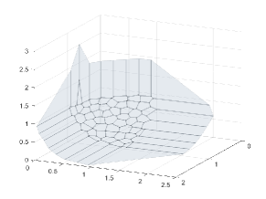
(a) Example 8.1 with $\epsilon=0.01$

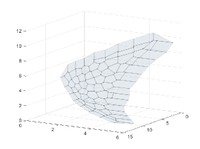
(b) Example 8.2 with $\epsilon=0.05$

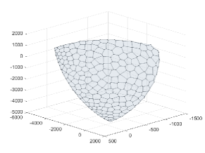
(c) Example 8.3 with $\epsilon=5$

Figure 1: Outer approximations obtained from Algorithm 1 using $\ell_{2}$ norm

Note that we could not run the algorithms in a few settings. We cannot solve Example 8.1, $q=4$ for $\epsilon=0.1$ by Algorithms 1 and 2 when $p=2$, and by Algorithms 2 and 3 when $p=\infty$. Similarly, we cannot solve Example 8.2 by Algorithm 3 for any $p\in\{1,2,\infty\}$. Moreover, we cannot solve this example by Algorithm 1 when $p=\infty$ for both $\epsilon$ values and when $p=1$ for $\epsilon=0.01$. Since it is not possible to provide a comparison, we do not report the results for $p=\infty$ in Table 2. Finally, Example 8.3 cannot be solved by Algorithms 1 and 2 when $p=1$. Hence, Table 3 does not show the results for $p=1$ for any setting. The main reason that the algorithms cannot solve these instances is the limitations of bensolve tools in vertex enumeration.

Table 1: Computational results for Example 8.1

		$q$=3							$q$=4
$p$	Alg	$\epsilon$	$\lvert\bar{\mathcal{X}}\rvert$	Opt	T${}_{\text{opt}}$	En	T${}_{\text{en}}$	T	$\epsilon$	$\lvert\bar{\mathcal{X}}\rvert$	Opt	T${}_{\text{opt}}$	En	T${}_{\text{en}}$	T
1	1	0.05	33	52	13.29	20	0.31	13.68	0.5	30	41	11.66	12	0.22	11.95
	2		42	59	15.59	17	0.26	15.99		57	69	19.27	11	0.28	19.71
	3		56	89	17.32	34	1.02	18.56		33	44	9.71	12	0.20	9.97
2	1		29	45	10.49	17	0.23	10.79		29	34	8.70	6	0.07	8.80
	2		44	61	14.24	17	0.24	14.68		94	99	25.98	5	0.07	26.20
	3		32	50	9.76	19	0.27	10.10		31	42	9.18	12	0.19	9.43
$\infty$	1		21	34	8.15	14	0.16	8.35		8	9	2.34	2	0.02	2.38
	2		37	51	12.39	13	0.15	12.61		11	15	4.23	1	0.02	4.39
	3		21	34	6.76	14	0.15	6.96		8	9	2.05	2	0.02	2.09
1	1	0.01	175	262	69.13	88	20.17	92.99	0.1	143	177	52.94	34	2.67	56.25
	2		161	235	62.55	73	10.56	75.28		232	273	78.37	38	5.05	84.42
	3		256	397	76.54	142	113.29	212.22		412	510	111.49	91	48.25	165.40
2	1		128	196	46.51	69	8.41	56.52		-
	2		145	209	49.42	64	6.56	57.29		-
	3		139	213	41.49	75	10.39	53.88		208	265	57.93	46	5.08	63.67
$\infty$	1		93	145	35.34	53	3.44	39.47		68	82	22.59	12	0.22	22.87
	2		107	154	37.20	47	2.43	40.15		-
	3		87	137	26.72	51	3.03	30.36		-

Table 2: Computational results for Example 8.2

$\epsilon$	$p$	Alg	$\lvert\bar{\mathcal{X}}\rvert$	Opt	T${}_{\text{opt}}$	En	T${}_{\text{en}}$	T
0.05	1	1	188	310	107.26	87	19.30	130.34
		2	157	233	79.79	70	9.88	91.94
	2	1	145	225	70.22	76	11.46	84.07
		2	141	206	61.72	64	7.18	70.47
0.01	1	1	-
		2	772	1187	401.00	340	3197.85	4276.37
	2	1	869	1421	420.01	311	2302.12	3171.41
		2	655	957	285.04	279	1529.54	2162.02

Table 3: Computational results for Example 8.3

			$n$=3						$n$=9
$\epsilon$	$p$	Alg	$\lvert\bar{\mathcal{X}}\rvert$	Opt	T${}_{\text{opt}}$	En	T${}_{\text{en}}$	T	$\lvert\bar{\mathcal{X}}\rvert$	Opt	T${}_{\text{opt}}$	En	T${}_{\text{en}}$	T
10	2	1	502	943	285.43	132	100.12	401.95	1561	2754	1159.60	225	753.05	2046.88
		2	958	3924	1194.30	137	122.28	1339.09	1770	4213	1819.70	218	733.58	2682.37
		3	305	965	259.85	164	211.23	502.43	2718	4520	1772.08	259	1324.24	3295.96
	inf	1	197	592	179.71	106	41.61	227.61	1231	2106	901.81	152	150.43	1076.14
		2	199	1206	390.99	100	36.67	432.99	3638	9222	4045.45	166	219.60	4301.63
		3	180	586	157.46	101	33.60	196.24	2628	5057	1994.39	164	202.33	2231.07
5	2	1	1178	3127	932.65	245	1059.10	2175.25	4461	7968	3371.91	390	8008.67	12795.23
		2	1207	5557	1702.79	259	1488.53	3441.28	7052	15662	6546.29	409	9908.03	18268.17
		3	579	3932	1049.79	309	3046.66	4529.37	7046	11149	4307.21	476	16898.76	23603.25
	inf	1	412	1740	526.33	185	325.59	907.19	3153	4538	1889.06	294	2164.45	4390.16
		2	465	2655	837.24	188	374.95	1268.01	3570	8155	3482.44	305	2589.99	6470.71
		3	342	1412	380.10	185	352.70	787.48	3146	4712	1845.91	300	2455.39	4663.98

In line with the theory, Tables 1-3 illustrate that Opt, En as well as T increase when a smaller approximation error is used, irrespective of the algorithm considered.

According to Table 1, for $p=1$ in terms of all performance measures, Algorithms 1 and 2 perform better than Algorithm 3, except for $q=4,\epsilon=0.5$ for which Algorithms 1 and 3 have similar performances. For $p\in\{2,\infty\}$, Algorithms 1 and 3 perform similar to each other and better than Algorithm 2 in terms of Opt, T${}_{\text{opt}}$ and T. When we compare Algorithms 1 and 2, we observe that Algorithm 2 solves a larger number of optimization problems (Opt) compared to Algorithm 1 in all settings except $p=1,\epsilon=0.01$. The reason may be that the former algorithm deals with a higher number of vertices, coming from the intersection of $\bar{\mathcal{P}}^{\text{out}}_{k}$ with $\operatorname{bd}S$, $k\geq 0$ (line 19 of Algorithm 2).

Table 2 indicates that, in solving Example 8.2, Algorithm 2 performs better than Algorithm 1 with respect to all indicators.

Finally, for Example 8.3 when we compare the performances under $n=3$ with $p=2$, Algorithm 1 works better compared to the others in terms of Opt, En and T. Under $n=3$ with $p=\infty$, the same holds for Algorithm 3, see Table 3. However, under $n=9$, Algorithm 1 performs better than the others in all instances.

When we compare the results for Example 8.3(a) and (b), we observe that even with the same precision level $\epsilon$, the number of minimizers is at least twice as and generally much higher than the number of minimizers in Example 8.3(a), which also affects the total times. The reason may be that due to the increase in the dimension of the feasible region and the structure of the objective functions, the range of the objective function changes and the difficulty of the problem increases in Example 8.3(b).

From the results of the test problems above, we deduce a comparable performance of our proposed algorithms compared to Algorithm 3.

Next, we consider Example 8.1 for $q\in\{2,3\}$ with different ordering cones than the positive orthant, see Table 4 and Figure 2. These cones are given below in terms of their generating vectors:

$$C_{1} =\operatorname{conv}\operatorname{cone}\{(1,2)^{\mathsf{T}},(2,1)^{\mathsf{T}}\},$$

$$C_{2} =\operatorname{conv}\operatorname{cone}\{(2,-1)^{\mathsf{T}},(-1,2)^{\mathsf{T}}\},$$

$$C_{3} =\operatorname{conv}\operatorname{cone}\{(4,2,2)^{\mathsf{T}},(2,4,2)^{\mathsf{T}},(4,0,2)^{\mathsf{T}},(1,0,2)^{\mathsf{T}},(0,1,2)^{\mathsf{T}},(0,4,2)^{\mathsf{T}}\},$$

$$C_{4} =\operatorname{conv}\operatorname{cone}\{(-1,-1,3)^{\mathsf{T}},(2,2,-1)^{\mathsf{T}},(1,0,0)^{\mathsf{T}},(0,-1,2)^{\mathsf{T}},(-1,0,2)^{\mathsf{T}},(0,1,0)^{\mathsf{T}}\}.$$

Note that we have $C_{1}\subsetneq\mathbb{R}^{2}_{+}\subsetneq C_{2}=C_{1}^{+}$ and $C_{3}$ $\subsetneq\mathbb{R}^{3}_{+}\subsetneq C_{4}=C_{3}^{+}$. We solve these examples with Algorithms 1 and 2, where the norm in (P$(v)$) is the $\ell_{2}$ norm. As before, due to the limitations of bensolve tools, Table 4 does not show the result for Algorithm 2 when the ordering cone is $C_{3}$ and $\epsilon=0.01$. According to Table 4, for $C_{1}$ and $C_{2}$, Algorithms 1 and 2 are comparable in terms of T. For $C_{3}$ with $\epsilon=0.05$, Algorithm 2 gives smaller T. However, for $C_{4}$, Algorithm 1 has better runtime.

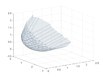
(a) $C_{3}$

(b) $C_{4}$

Figure 2: Outer approximations obtained from Algorithm 1 using $\ell_{2}$ norm for Example 8.1 with $q=3$ under different cones

Table 4: Computational results for Example 8.1 with different ordering cones and $p=2$

		$q$ = 2								$q$ = 3
Alg	$\epsilon$	$C$	$\lvert\bar{\mathcal{X}}\rvert$	Opt	T${}_{\text{opt}}$	En	T${}_{\text{en}}$	T	$\epsilon$	$C$	$\lvert\bar{\mathcal{X}}\rvert$	Opt	T${}_{\text{opt}}$	En	T${}_{\text{en}}$	T
1	0.005	$C_{1}$	19	34	6.95	16	0.12	7.12	0.05	$C_{3}$	62	89	20.54	28	0.79	21.50
2			21	36	7.51	15	0.11	7.69			57	77	18.27	18	0.35	18.82
1		$C_{2}$	6	9	1.87	4	0.02	1.91		$C_{4}$	22	29	6.57	8	0.08	6.68
2			8	11	2.30	3	0.02	2.36			28	34	7.90	4	0.04	8.01
1	0.001	$C_{1}$	37	69	14.39	32	0.45	14.96	0.01	$C_{3}$	229	346	80.66	117	62.00	154.04
2			36	67	14.09	31	0.44	14.69			-
1		$C_{2}$	10	17	3.44	8	0.05	3.52		$C_{4}$	71	107	24.99	37	1.45	26.78
2			12	19	4.04	7	0.04	4.13			90	123	28.94	31	1.05	30.31

We conclude this section by a remark that illustrates the necessity of intersecting $\bar{\mathcal{P}}_{k}^{\text{out}}$ with $S$ in Algorithm 2.

Remark 8.4.

As noted before in Section 6, it is possible that some vertices of $\bar{\mathcal{P}}_{k}^{\text{out}}$ falls outside $S$. Consider Example 8.1 with $q=3$. Note that $\Gamma(\mathcal{X})$ is the unit ball centered at $e\in\mathbb{R}^{3}$, and $\mathcal{P}_{0}$ is the positive orthant. In the initialization phase of Algorithm 2, we obtain $S=\{y\in\mathbb{R}^{3}\mid\bar{w}^{\mathsf{T}}y\leq 3.56\}$, where $\bar{w}=\frac{1}{\sqrt{3}}e$. For illustrative purposes, consider the supporting halfspace $\mathcal{H}=\{y\in\mathbb{R}^{q}\mid w^{\mathsf{T}}y\geq 0.68\}$ of the upper image, where the normal direction is $w=(1,1,0.1)^{\mathsf{T}}$. This would support the upper image at the $C$-minimal point $(0.2947,0.2947,0.9295)^{\mathsf{T}}$. Note that $\operatorname{bd}\mathcal{H}$ intersects with $\mathcal{P}_{0}$ to give three vertices: $v^{1}=(0.68,0,0)^{\mathsf{T}}$, $v^{2}=(0,0.68,0)^{\mathsf{T}}$, $v^{3}=(0,0,6.8)^{\mathsf{T}}$. Clearly, $v^{1},v^{2}\in S$ and $v^{3}\notin S$. Moreover, as stated in Remark 6.5 the approximation generated by $v^{1},v^{2}$, namely, $\operatorname{conv}(\{v^{1},v^{2}\})+\mathbb{R}_{+}^{3}$ does not contain the upper image; see Figure 3.

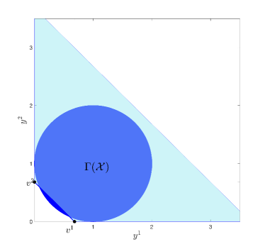
Figure 3: Projections of $\Gamma(\mathcal{X})$ (dark blue), $\operatorname{conv}(\{v^{1},v^{2}\})+\mathbb{R}_{+}^{3}$ (light blue) from Remark 8.4 on the $y_{3}=0$ plane

We practically encounter vertices which fall outside $S$, for instance, while running Algorithm 1 for Example 8.1 with $q=3$, $p=2$ and $\epsilon=0.01$. Figure 4 shows the outer approximation, after iteration $k=37$, with one of the vertices outside $\mathcal{P}_{0}^{\text{out}}\cap S$.

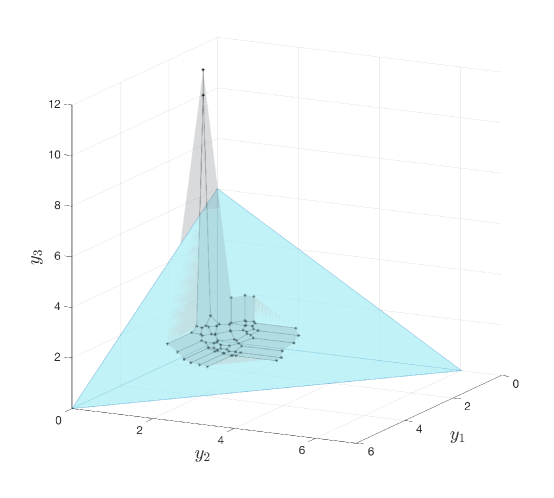
Figure 4: Outer approximation $\mathcal{P}_{k}^{\text{out}}$, $k=37$ (vertices and representative points on unbounded edges indicated by black markers) for Example 8.1 obtained using Algorithm 1 (for $p=2$ and $\epsilon=0.01$) has one vertex outside $S$ (blue).

9 Conclusions

In this study, we have proposed an algorithm for CVOPs which is based on a norm-minimizing scalarization. It is different from the similar class of algorithms available in the literature in the sense that it does not need a direction parameter as an input. We have also proposed a modification of the algorithm and proved its finiteness under the assumption of compact feasible region. Using benchmark test problems, the computational performance of the new algorithms is found to be comparable to a CVOP algorithm in the recent literature which uses the Pascoletti-Serafini scalarization.

References

- [1] Charalambos D. Aliprantis and Kim C. Border. Infinite Dimensional Analysis: A Hitchhiker’s Guide. Springer, 2006.
- [2] Çağın Ararat, Özlem Çavuş, and Ali İrfan Mahmutoğulları. Multi-objective risk-averse two-stage stochastic programming problems. arXiv preprint 1711.06403, 2017.
- [3] Harold P. Benson. Concave minimization: theory, applications and algorithms. In Reiner Horst and Panos M Pardalos, editors, Handbook of Global Optimization, pages 43–148. Springer, 1995.
- [4] Harold P. Benson. An outer approximation algorithm for generating all efficient extreme points in the outcome set of a multiple objective linear programming problem. Journal of Global Optimization, 13(1):1–24, 1998.
- [5] Harold P. Benson and Reiner Horst. A branch and bound-outer approximation algorithm for concave minimization over a convex set. Computers & Mathematics with Applications, 21(6-7):67–76, 1991.
- [6] Stephen P. Boyd and Lieven Vandenberghe. Convex Optimization. Cambridge University Press, 2004.
- [7] Regina Sandra Burachik, C. Yalçın Kaya, and M. M. Rizvi. A new scalarization technique and new algorithms to generate pareto fronts. SIAM Journal on Optimization, 27(2):1010–1034, 2017.
- [8] Fennell Burns, Miroslav Fiedler, and Emilie Haynsworth. Polyhedral cones and positive operators. Linear Algebra and its Applications, 8(6):547–559, 1974.
- [9] Aura Conci and Carlos Kubrusly. Distances between sets - a survey. Advances in Mathematical Sciences and Applications, 26(1), 2017.
- [10] Marianna De Santis, Gabriele Eichfelder, Julia Niebling, and Stefan Rocktäschel. Solving multiobjective mixed integer convex optimization problems. SIAM Journal on Optimization, 30(4):3122–3145, 2020.
- [11] Daniel Dörfler, Andreas Löhne, Christopher Schneider, and Weißing Benjamin. A Benson-type algorithm for bounded convex vector optimization problems with vertex selection. Optimization Methods and Software, 2021.
- [12] Matthias Ehrgott. Multicriteria Optimization, volume 491. Springer Science & Business Media, 2005.
- [13] Matthias Ehrgott, Lizhen Shao, and Anita Schöbel. An approximation algorithm for convex multi-objective programming problems. Journal of Global Optimization, 50(3):397–416, 2011.
- [14] Matthias Ehrgott and Margaret M. Wiecek. Mutiobjective programming. In José Figueira, Salvatore Greco, and Matthias Ehrgott, editors, Multiple Criteria Decision Analysis: State of the Art Surveys, pages 667–708. Springer, 2005.
- [15] Gabriele Eichfelder. Adaptive Scalarization Methods in Multiobjective Optimization. Springer, 2008.
- [16] James P. Evans and Ralph E. Steuer. A revised simplex method for linear multiple objective programs. Mathematical Programming, 5(1):54–72, 1973.
- [17] Francisco Facchinei and Jong-Shi Pang. Finite-Dimensional Variational Inequalities and Complementarity Problems. Springer Science & Business Media, 2007.
- [18] Zachary Feinstein and Birgit Rudloff. A recursive algorithm for multivariate risk measures and a set-valued bellman’s principle. Journal of Global Optimization, 68, 2017.
- [19] Michael C. Grant and Stephen P. Boyd. Graph implementations for nonsmooth convex programs. In Vincent D. Blondel, Stephen P. Boyd, and Hidenori Kimura, editors, Recent Advances in Learning and Control, Lecture Notes in Control and Information Sciences, pages 95–110. Springer-Verlag Limited, 2008. http://stanford.edu/~boyd/graph_dcp.html.
- [20] Michael C. Grant and Stephen P. Boyd. CVX: Matlab software for disciplined convex programming, version 2.2., 2020.
- [21] Frank Heyde and Andreas Löhne. Solution concepts in vector optimization: a fresh look at an old story. Optimization, 60(12):1421–1440, 2011.
- [22] Johannes Jahn. Scalarization in vector optimization. Mathematical Programming, 29(2):203–218, 1984.
- [23] Johannes Jahn. Vector Optimization. Springer, 2nd edition, 2011.
- [24] Refail Kasimbeyli, Zehra Kamisli Ozturk, Nergiz Kasimbeyli, Gulcin Dinc Yalcin, and Banu Icmen Erdem. Comparison of some scalarization methods in multiobjective optimization. Bulletin of the Malaysian Mathematical Sciences Society, 42(5):1875–1905, 2019.
- [25] Akhtar A. Khan, Christiane Tammer, and Constantin Zălinescu. Set-valued Optimization: An Introduction with Applications. Springer, 2016.
- [26] JiGuan G. Lin. On min-norm and min-max methods of multi-objective optimization. Mathematical Programming, 103(1):1–33, 2005.
- [27] C. G. Liu, K. F. Ng, and W. H. Yang. Merit functions in vector optimization. Mathematical Programming, 2009.
- [28] Andreas Löhne. Vector Optimization with Infimum and Supremum. Springer Science & Business Media, 2011.
- [29] Andreas Löhne, Birgit Rudloff, and Firdevs Ulus. Primal and dual approximation algorithms for convex vector optimization problems. Journal of Global Optimization, 60(4):713–736, 2014.
- [30] Andreas Löhne and Andrea Wagner. Solving DC programs with a polyhedral component utilizing a multiple objective linear programming solver. Journal of Global Optimization, 69(2):369–385, 2017.
- [31] Andreas Löhne and Benjamin Weißing. Equivalence between polyhedral projection, multiple objective linear programming and vector linear programming. Mathematical Methods of Operations Research, 84(2):411–426, 2016.
- [32] Andreas Löhne and Benjamin Weißing. The vector linear program solver bensolve–notes on theoretical background. European Journal of Operational Research, 260(3):807–813, 2017.
- [33] Dinh The Luc. Theory of Vector Optimization. Springer, 1989.
- [34] Kaisa Miettinen. Nonlinear Multiobjective Optimization, volume 12. Springer Science & Business Media, 2012.
- [35] Kaisa Miettinen, Marko M. Mäkelä, and Katja Kaario. Experiments with classification-based scalarizing functions in interactive multiobjective optimization. European Journal of Operational Research, 175(2):931–947, 2006.
- [36] Boris S. Mordukhovich and Nguyen Mau Nam. An easy path to convex analysis and applications. Synthesis Lectures on Mathematics and Statistics, 6(2):1–218, 2013.
- [37] Soghra Nobakhtian and Narjes Shafiei. A Benson type algorithm for nonconvex multiobjective programming problems. TOP, 25(2):271–287, 2017.
- [38] Adriano Pascoletti and Paolo Serafini. Scalarizing vector optimization problems. Journal of Optimization Theory and Applications, 42(4):499–524, 1984.
- [39] R. Tyrrell Rockafellar. Convex Analysis, volume 28. Princeton university press, 1970.
- [40] Birgit Rudloff and Firdevs Ulus. Certainty equivalent and utility indifference pricing for incomplete preferences via convex vector optimization. Mathematics and Financial Economics, 15:397–430, 2021.
- [41] Birgit Rudloff, Firdevs Ulus, and Robert Vanderbei. A parametric simplex algorithm for linear vector optimization problems. Mathematical Programming, 163(1-2):213–242, 2017.
- [42] Stefan Ruzika and Margaret M. Wiecek. Approximation methods in multiobjective programming. Journal of Optimization Theory and Applications, 126(3):473–501, 2005.
- [43] Milan Zeleny. Compromise programming. In Milan Zeleny and James L. Cochrane, editors, Multiple Criteria Decision Making, pages 373–391. University of South Carolina Press, 1973.