Discrete Vector Bundles with Connection and the Bianchi Identity

Abstract.

We develop a combinatorial theory of vector bundles with connection that is natural with respect to appropriate mappings of the base space. The base space is a simplicial complex, the main objects defined are discrete vector bundle valued cochains and the main operators we develop are a discrete exterior covariant derivative and a combinatorial wedge product. Key properties of these operators are demonstrated and it is shown that they are natural with respect to the mappings referred to above. We also formulate a well-behaved definition of metric compatible discrete connections. A characterization is given for when a discrete vector bundle with connection is trivializable or has a trivial lower rank subbundle. This machinery is used to define discrete curvature as linear maps and we show that our formulation satisfies a discrete Bianchi identity. Recently an alternative framework for discrete vector bundles with connection has been given by Christiansen and Hu. We show that our framework reproduces and extends theirs when we apply our constructions on a subdivision of the base simplicial complex.

1. Introduction

Some numerical approaches to partial differential equations rely on combinatorial models for differential geometric objects. These models often encode intricate structures that are of interest from a purely mathematical point of view. Such structures are particularly rich if one demands that algebraic identities from geometry be faithfully encoded in the combinatorial model.

A fundamental example comes from the algebraic identities relating the divergence, gradient, and curl. These identities can be phrased (and generalized) in terms of the exterior derivative and Hodge star operators acting on differential forms. There are robust combinatorial models for the Hodge-de Rham complex in which the standard algebraic identities hold, e.g., $d\circ d=0$ and the Leibniz rule [15, 2, 3, 22, 42]. These combinatorial models have met success in a wide variety of applications, e.g., computational electromagnetism [7, 21], elasticity [5, 4, 30], numerical relativity [37, 30], fluid mechanics [25, 31, 35, 34, 26, 40], quantum electrodynamics [36] and many other areas of physics and geometry [1]. Contemplating the ensuing combinatorial wedge product leads to ever more sophisticated algebraic structures whose utility depends on the desired application. For example, the failure of the combinatorial wedge to be associative leads to $A_{\infty}$-structures, e.g., see [20, 18, 17].

This paper initiates a generalization of these combinatorial models to differential forms with values in a vector bundle with connection. Specifically, we construct a combinatorial exterior covariant derivative and combinatorial wedge product that satisfy the algebraic identities one expects, e.g., the Bianchi identity. Out of these definitions emerges a combinatorial expression of curvature which also behaves as one expects: curvature measures the failure of parallel transport to be independent of the path, and is the local obstruction to a trivialization.

One of the eventual goals of this theory is the development of coordinate-independent numerical methods for partial differential equations. Of particular interest are Einstein’s equation and the Yang–Mills equations. These examples require a framework beyond a combinatorial Hodge-de Rham complex. In this paper, we explore one such framework, that of connections on vector bundles. A related direction is to combine complexes to create new complexes using Bernstein-Gelfand-Gelfand (BGG) constructions [1, 8]. This yields various elasticity complexes (e.g. the Kröner complex, also known as the linearized Calabi complex in geometry), the Hessian and div-div complexes that are used for biharmonic problems and Einstein equations and an approach to construct differential complexes with higher order differentials [1]. One potential application of our framework is in combinatorial discretization of vector de Rham complexes that are used extensively in the BGG construction. Another avenue could be the formulation of a BGG-type construction in the discrete setting for the case of non-flat connections. Hints of the relationship between BGG and discrete vector bundles are in the related discrete vector bundle construction of Christiansen and Hu [13].

Just as there are multiple approaches to the combinatorial de Rham complex, there are multiple approaches to its generalizations. In all cases, one combines structures in a preferred combinatorial model of the de Rham complex with ideas from lattice gauge theory following Wilson [41] (see also [32]). Our approach generalizes discrete exterior calculus (DEC), a combinatorial model for the de Rham complex that encodes algebraic identities and also can be directly compared to finite element methods; see §2 below. With this direct comparison to established numerical methods, we expect the theory developed below to be amenable to applications in physics and engineering.

A related theory for combinatorial covariant exterior derivatives (but not the wedge product) has been recently developed by Christiansen and Hu [13]. In §11 we show that their constructions can be extracted and extended by applying our theory to a special class of simplicial complexes. On these complexes, aspects of the combinatorial constructions can be made more elegant. Some aspects of [13] can be viewed as a new approach to simplicial gauge theory and this is the latest in a series of papers on computational gauge theory and related topics by Christiansen and co-authors which combine ideas from lattice gauge theory and finite element methods [9, 11, 12, 10]. A recent finite element based approach to discretization of Levi-Civita connection is in [6].

Review of vector bundle valued forms in smooth geometry

Let $E$ be a vector bundle over a smooth manifold $M$. Consider the vector space of $E$-valued differential $k$-forms $\Lambda^{k}(M;E)$ and the graded vector space $\Lambda^{\bullet}(M;E)\cong\bigoplus_{k}\Lambda^{k}(M;E)$ of $E$-valued forms. The graded algebra $\Lambda^{\bullet}(M)$ of differential forms acts on $\Lambda^{\bullet}(M;E)$ through linear maps

(1) $$\Lambda^{k}(M;E)\times\Lambda^{l}(M)\to\Lambda^{k+l}(M;E),\qquad(\alpha,w)\mapsto\alpha\wedge w$$

for each $k$ and $l$. If we equip $E$ with a connection $\nabla\colon\Gamma(E)\to\Lambda^{1}(M;E)$, the exterior covariant derivative extends $\nabla$ to a degree +1 map $d_{\nabla}$ on $E$-valued forms

(2) $$\Gamma(E)=\Lambda^{0}(M;E)\stackrel{{\scriptstyle\nabla=d_{\nabla}}}{{\longrightarrow}}\Lambda^{1}(M;E)\stackrel{{\scriptstyle d_{\nabla}}}{{\to}}\Lambda^{2}(M;E)\stackrel{{\scriptstyle d_{\nabla}}}{{\to}}\Lambda^{3}(M;E)\to\cdots$$

This extension $d_{\nabla}$ is designed to be compatible with the de Rham differential $d\colon\Lambda^{k}(M)\to\Lambda^{k+1}(M)$ by way of the Leibniz rule,

(3) $$d_{\nabla}(\alpha\wedge w)=d_{\nabla}\alpha\wedge w+(-1)^{|\alpha|}\alpha\wedge dw.$$

When $E$ is the trivial line bundle and $\nabla$ is the trivial connection, we have $(\Lambda^{k}(M;E),d_{\nabla})=(\Lambda^{k}(M),d)$, and (3) becomes the usual Leibniz rule for the de Rham differential. For a general connection, one important difference from the de Rham complex is that $d_{\nabla}\circ d_{\nabla}$ need not be zero, and hence (2) need not be a cochain complex. Indeed, the vanishing of $d_{\nabla}\circ d_{\nabla}$ is equivalent to $\nabla$ being a flat connection. The failure of flatness is measured by the operator

(4) $$F:=d_{\nabla}\circ d_{\nabla}\in\Lambda^{2}(M;{\rm End}(E))$$

called the curvature of $\nabla$, where the endomorphism bundle ${\rm End}(E)$ is the vector bundle over $M$ whose fiber at $x$ is the space of linear endomorphisms of the fiber $E_{x}$. The curvature $F$ acts on $E$-valued forms via the linear maps

(5) $$F\colon\Lambda^{k}(M;E)\to\Lambda^{k+2}(M;E).$$

The structures (1)-(5) are natural in the manifold $M$: a smooth map $f\colon N\to M$ determines a map of the sequences (2) for $E$ on $M$ and $f^{\ast}E$ on $N$ using the connections $\nabla$ and $f^{\ast}\nabla$. This map is compatible with the induced map of de Rham complexes and the curvature of $f^{*}\nabla$ is $f^{*}F$, the pullback of the curvature of $\nabla$. Furthermore, $d_{\nabla}$ commutes with $f^{*}$ in the sense that $f^{*}d_{\nabla}=d_{f^{*}\nabla}f^{*}$, and similarly the wedge product commutes with $f^{*}$. This generalizes naturality of the de Rham complex.

Statement of results

This paper develops a theory of discrete vector bundles with connection over simplicial complexes with properties mirroring (1)-(5) that are appropriately natural with respect to maps of simplicial complexes. We constraint the theory by requiring that it specialize to the metric-free part of DEC in the case of a trivial bundle with trivial connection.

We now summarize our two main theorems. One concerns the structure preserving discretization of the framework for differential geometry using vector bundles described above. The second result is about the application of this discrete framework to trivializability and reduction of structure group. We state the theorems below and prove these in various propositions later in the paper. The terminology used is defined later in the appropriate sections. Additional results relating our framework to that of Christiansen and Hu [13] are in §11.

Theorem 1.1 (Structure-preserving discretization).

Let $X^{\prime}$ and $X$ be simplicial complexes, $(E,\nabla)$ a discrete vector bundle with connection over $X$, and $f:X^{\prime}\to X$ an abstract simplicial map. We construct operations

$$F \in C^{2}(X;{\rm Hom}(E))$$

$$\nabla :\Gamma(E)=C^{0}(X;E)\to C^{1}(X;E)$$

$$d_{\nabla} :C^{k}(X;E)\to C^{k+1}(X;E)$$

$$\wedge :C^{k}(X;E)\times C^{l}(X)\to C^{k+l}(X;E)$$

$$C^{k}(X ;{\rm Hom}(E))\times C^{l}(X;E)\to C^{k+l}(X;E)$$

$$d_{\nabla} :C^{k}(X;{\rm Hom}(E))\to C^{k+1}(X;{\rm Hom}(E))$$

such that

1. (Leibniz rule, Proposition 7.2, Cor. 7.3) For $\alpha\in C^{k}(X;E)$ and $w\in C^{l}(X)$, and $k,l$ nonnegative integers

   $$d_{\nabla}(\alpha\wedge w)=d_{\nabla}\alpha\wedge w+(-1)^{k}\alpha\wedge dw\,,$$

2. (Naturality, Proposition 6.3 and 7.4) $f^{\ast}(\alpha\wedge w)=f^{\ast}\alpha\wedge f^{\ast}w$, and $f^{\ast}d_{\nabla}=d_{f^{\ast}\nabla}f^{\ast}$,

3. (Curvature, Proposition 8.7) $d_{\nabla}d_{\nabla}\alpha=F\;\alpha$, and

4. (Bianchi identity, Proposition 8.8) $d_{\nabla}F=0$.

The naturality results above reduce to results about DEC for a real line bundle and trivial connection.

In the case of a bundle with metric, we show in Proposition 7.8 that metric compatibility of the discrete connection is equivalent to a Leibniz rule.

We define a flat discrete connection $\nabla$ to be one for which parallel transport is the same for simple homotopic paths. On the other hand, the curvature $F$ of the connection is defined as $d_{\nabla}^{2}$. The following shows vanishing curvature is equivalent to a flat connection, and furthermore that curvature obstructs trivializability.

Theorem 1.2 (Trivializability, Cor. 4.11 and Proposition 8.5).

Given a discrete vector bundle with connection $(E,\nabla)$ over a simply connected simplicial complex $X$, the following are equivalent: (i) $(E,\nabla)$ is trivializable; (ii) $(E,\nabla)$ is flat; and (iii) $F=0$.

The above follows from a result for connected but (possibly) not simply connected simplicial complexes, namely that a flat discrete vector bundle with connection is determined by a homomorphism out of its fundamental group, $\pi_{1}(X)\to{\rm GL}_{n}$.

In §5 we also describe conditions under which a bundle can be trivialized only partially, e.g., when it admits a trivializable subbundle. We phrase these results in terms of reduction of structure group relative to a subgroup $G<{\rm GL}_{n}$. Reduction to $\{e\}<{\rm GL}_{n}$ is equivalent to trivializability.

The relationship between the discrete vector bundle constructions of Christiansen and Hu [13] and our constructions are summarized in Proposition 11.1. An interesting fact in this context is the relationship between Leibniz rule and discrete curvature which is discussed in §9 and §11.5. In Proposition 11.18, under appropriate hypotheses, we show Leibniz rule for a wedge product that we define for a slight extension of the discrete vector bundle construction of Christiansen and Hu.

2. Background: Discrete exterior calculus and naturality

DEC is a combinatorial framework for discretizing scalar-valued differential forms and exterior calculus operators in a way that faithfully encodes expected algebraic identities, e.g., the Leibniz rule for the de Rham differential. Riemannian metric is encoded in DEC via a primal and dual cell complex incorporating orthogonality and lengths, areas, volumes etc.

The input data for DEC is a simplicial complex $X$ with additional decorations and properties. The discrete notions of differential form, exterior derivative, and wedge product only depend on the simplicial complex, importing standard methods from simplicial algebraic topology. When incorporating features that depend on a metric (e.g., a discretization of the Hodge star operator) essentially one requires that $X$ approximates a manifold. This assumption is appropriate given the desired applications: DEC has been used mostly as a method for solving partial differential equations (PDEs) on simplicial approximations of embedded orientable manifolds.

With the above in mind, below we will assume that $X$ arises as an approximation of an embedded manifold. In particular, each top dimensional simplex is embedded in $\mathbb{R}^{N}$ individually, and combinatorial data specifies how these are glued to each other. This may be presented by embedding the entire approximation of the manifold as a complex of dimension $n$ embedded in $\mathbb{R}^{N}$ for some $N\geq n$. A common example is a piecewise-linear (PL) approximation of a surface in $\mathbb{R}^{3}$. But the coordinate-independent aspect of DEC does not require such a global embedding. All the operations and objects are local to the simplices and their neighbors. In DEC, the top dimensional simplices of the simplicial approximation of an orientable manifold are oriented consistently and the lower dimensional simplices are oriented arbitrarily.

For simplicial complexes $X$ and $Y$ recall that an abstract simplicial map $f\colon X\to Y$ is of the form $f(\{v_{0},\ldots,v_{k}\})=\{f^{(0)}(v_{0}),\ldots,f^{(0)}(v_{k})\}$ for some map $f^{(0)}:X^{(0)}\to Y^{(0)}$ (called the vertex map of $f$) such that $v_{0},\ldots v_{k}$ spanning a simplex in $X$ implies $f(\{v_{0},\ldots,v_{k}\})$ spans one in $Y$. See for instance [29]. For us, abstract simplicial maps will be analogous maps between ordered simplices. That is, the sets $\{v_{0},\ldots,v_{k}\}$ (simplices) above are replaced by ordered sets $[v_{0},\ldots,v_{k}]$ (oriented simplices).

Given a differential form $\alpha\in\Lambda^{k}(M)$, its discrete analog in DEC is the $k$-cochain $\int_{\textvisiblespace}\alpha$ which takes values in $\mathbb{R}$ when evaluated on $k$-dimensional chains, that is, the result of a de Rham map [16]. The space of real-valued $k$-cochains on simplicial complex $X$ will be denoted $C^{k}(X)$. The coboundary operator on cochains plays the role of discrete exterior derivative ($d$), the cup product ($\smile$) plays the role of tensor product and the antisymmetrized cup product plays the role of a discrete wedge product ($\wedge$). Thus $d$ satisfies a Leibniz rule with respect to $\wedge$ since the coboundary operator does so with respect to $\smile$. Discrete Hodge star construction involves a Poincaré dual complex of $X$ using circumcenters and is not relevant to this paper. See [22] for details.

The discrete $d$ and $\wedge$ commute with pullback by abstract simplicial maps. Thus such maps play the role that smooth maps play in calculus on smooth manifolds.

3. Discrete Vector Bundles with Connection

Definition 3.1.

Given a simplicial complex $X$, a real (respectively, complex) discrete vector bundle with connection over $X$ consists of the following:

1. for each vertex $i\in X^{(0)}$, a finite-dimensional real (respectively, complex) vector space $E_{i}$ called the fiber at $i$; and

2. for each edge $[ij]\in X^{(1)}$, an invertible linear map $U_{ji}\colon E_{i}\to E_{j}$ called parallel transport from $i$ to $j$.

We require the compatibility condition that $U_{ij}=U_{ji}^{-1}$.

Sometimes we will refer to a discrete vector bundle with connection over $X$ simply as a vector bundle over $X$. The rank of a vector bundle on a connected component of $X$ is the (necessarily constant) dimension of the fibers. Given a subcomplex $Y\subset X$, the restriction of a bundle is a discrete vector bundle with connection gotten from the obvious restriction of the data (1) and (2) above.

We note that one is always free to choose a basis for the vector space at each fiber, giving isomorphisms $\mathbb{R}^{n}\cong E_{i}$ or $\mathbb{C}^{n}\cong E_{i}$ for each $i$. Borrowing terminology from the physics literature, we refer choices of such isomorphisms as a choice of gauge. After a choice of gauge has been made, the parallel transport maps are determined by matrices in ${\rm GL}_{n}(\mathbb{R})$ for real vector bundles or ${\rm GL}_{n}(\mathbb{C})$ for complex vector bundles. Below we use the notation ${\rm GL}_{n}$ to denote either ${\rm GL}_{n}(\mathbb{R})$ or ${\rm GL}_{n}(\mathbb{C})$, i.e., for statements that hold over both $\mathbb{R}$ and $\mathbb{C}$.

The notion of a discrete vector bundle without connection is not a particularly useful one: dropping the parallel transport maps gives vector spaces $E_{i}$ at each vertex that have no geometric relationship with each other.

Definition 3.2.

Let $X$ be a simplicial complex with a total ordering on the vertices. For each $k$-simplex in $X$, we choose the lowest numbered vertex to be the origin vertex of the $k$-simplex. With this choice fixed for all $k$-simplices in $X$, a vector bundle valued $k$-cochain $\alpha$ assigns to each oriented $k$-simplex $\sigma$ of $X$ a vector $\langle\alpha,\sigma\rangle_{l}\in E_{l}$ where $l$ is the origin vertex of $\sigma$. The evaluation on $\sigma$ with the opposite orientation is required to return the same value but with the opposite sign. The vector space of $k$-cochains is denoted $C^{k}(X;E)$. A section $s$ is a vector bundle valued 0-cochain, i.e., a vector $s_{i}\in E_{i}$ for each vertex.

Remark 3.3.

We describe how origin vertices arise when discretizing smooth objects. Let $E\to M$ be a smooth vector bundle over a smooth manifold $M$ with a chosen oriented triangulation. We discretize a smooth vector bundle valued differential $k$-form $\hat{\alpha}\in\Lambda^{k}(M;E)$ as follows. For each $k$-simplex $\mathbb{R}^{k}\supseteq\sigma\hookrightarrow M$, choose a vertex $l\in\sigma$, and an orientation of the vector space $E_{l}$ (which is canonical if the vector bundle $E\to M$ is oriented). There is a linear contracting homotopy from $\sigma$ to $l$ that gives an isomorphism of vector bundles $E|_{\sigma}\simeq\sigma\times E_{l}$ over $\sigma$. This isomorphism identifies the restriction $\hat{\alpha}|_{\sigma}$ with a vector space valued differential form $\hat{\alpha}|_{\sigma}\in\Lambda^{k}(\sigma;E_{l})$, for which the integral $\int_{\sigma}\hat{\alpha}$ is well-defined. Define the $k$-cochain $\alpha\in C^{k}(X;E)$ by the formula $\langle\alpha,\sigma\rangle_{l}:=\int_{\sigma}\hat{\alpha}\in E_{l}$. The cochain $\alpha\in C^{k}(X;E)$ is the discretization of $\hat{\alpha}$ relative to the chosen origin vertices $l\in\sigma$ for each $\sigma\hookrightarrow M$. We note that the discretization of a section $\hat{\alpha}\in\Lambda^{0}(M;E)=\Gamma(E)$ is canonical, but for $k>0$ the discretization depends on a choice of origin vertex.

Origin vertices can be recorded in a number of ways. Below, we will choose a total ordering on the vertices of $X$ and then take the lowest numbered vertex in each simplex as the origin for that simplex. (However, see Remark 3.4 below.) Hence, our computations will depend on this choice; however, on a given simplex computations only depend on the choices of origins on sub-simplices. When a global ordering is fixed, or the origin vertices are clear from context, the subscript $l$ in $\langle\alpha,\sigma\rangle_{l}$ from Definition 3.2 will be dropped.

Remark 3.4.

A priori, choices of origin vertex are additional data, possibly determined by the total ordering on vertices. However, certain triangulations can have canonical origin vertices without requiring a total ordering on vertices. One such structure is obtained via a subdivision and is used starting in §10. Such a structure is an important piece of the approach to discrete vector bundles with connection taken by Christiansen and Hu [13]; we discuss how their framework fits with ours in §11. We first develop our framework in this section and §6-9 with the assumption of a total ordering on vertices and then drop this restriction starting in §10.

In addition to their natural role in discretizing smooth objects, particular choices of origin vertices (such as the one we have chosen) appear to be useful in avoiding a curvature obstruction to Leibniz rule. See §9 and §11.5.

For $\tau\in S_{k+1}$ a permutation and $\sigma=[v_{0},\ldots,v_{k}]$ an oriented simplex, let $\tau(\sigma)$ be the oriented simplex $[v_{\tau(0)},\ldots,v_{\tau(k)}]$. We have the formula $\langle\alpha,\tau(\sigma)\rangle_{l}=\operatorname{sgn}(\tau)\langle\alpha,\sigma\rangle_{l}$ relating the evaluations, where $\operatorname{sgn}(\tau)$ is the sign of the permutation $\tau$.

In constructions we will often need to transport the value of a $k$-cochain to a (non-origin) vertex. We use the notation

$$\langle\alpha,\sigma\rangle_{i}:=U_{il}\langle\alpha,\sigma\rangle_{l}\in E_{i},$$

where the origin vertex of $\sigma$ is $l$.

In what follows we will often write $i$ for vertex $v_{i}$ and dispense with the commas unless needed. Thus the oriented simplex $[v_{0},\ldots,v_{k}]$ may be written as $[0\,...\,k]$, an edge $[v_{i},v_{j}]$ may be written as $[ij]$ etc. In examples, the value $\langle\alpha,[v_{0},\ldots,v_{k}]\rangle_{l}$ of a cochain may be shortened to $\alpha_{0\,...\,k}$ when $l$ is clear from the context or is not important.

Definition 3.5.

The covariant derivative (or connection) is a map $\nabla\colon C^{0}(X;E)\to C^{1}(X;E)$ which to a section $s$ assigns the vector bundle valued 1-cochain defined by its value on edges $[ij]$ by

(6) $$\langle\nabla s,[ij]\rangle_{i}:=U_{ij}s_{j}-s_{i}\in E_{i}.$$

The defining feature of the covariant derivative in smooth geometry is a Leibniz rule with respect to multiplying a section of a bundle by a function on the base. In our discrete setting this is proved in Proposition 7.2 after we have introduced a discrete wedge product and therefore justifies our terminology in the above definition.

The covariant derivative completely determines the data (2) in Definition 3.1. As such, following the convention in differential geometry we use the notation $(E,\nabla)$ to refer to a discrete vector bundle with connection over a simplicial complex $X$.

Definition 3.6.

Let $f\colon X\to X^{\prime}$ be an abstract simplicial map, $(E,\nabla)$ a discrete vector bundle with connection over $X$, and $(E^{\prime},\nabla^{\prime})$ be a discrete vector bundle with connection over $X^{\prime}$. A map of discrete vector bundles covering $f$, denoted $\tilde{f}\colon(E,\nabla)\to(E^{\prime},\nabla^{\prime})$, is a collection of linear maps $\tilde{f}_{l}\colon E_{l}\to E^{\prime}_{f(l)}$, one for each $l\in X^{(0)}$ so that the following diagram commutes

whenever there is an edge from vertex $i$ to $j$. In particular, if an edge $[ij]$ in $X$ is sent to a vertex in $X^{\prime}$ under $f$ (so $f(i)=f(j)$), we assign $U_{f(j),f(i)}=\operatorname{Id}_{E_{f(i)}}$ to be the identity map.

A map of discrete vector bundles with connection is an isomorphism if the simplicial map $f\colon X\to X^{\prime}$ is an isomorphism and $\tilde{f}_{i}:E_{i}\to E^{\prime}_{f(i)}$ is an isomorphism for all $i\in X^{(0)}$. An isomorphism of $(E,\nabla)$ covering the identity map on $X$ is called an automorphism of $(E,\nabla)$. If a choice of gauge has been fixed, then an automorphism is also called a gauge transformation.

We note that a gauge transformation is specified by the data of an element of ${\rm GL}_{n}$ at each vertex.

Example 3.7.

We explain how gauge transformations act on parallel transport matrices by way of an example. Consider the 1-dimensional simplicial complex $X$ with three vertices $0,1,2$ and three edges $[01],[12],[02]$, i.e., a triangle. A discrete vector bundle with connection on $X$ is the data of three vector spaces $E_{i}$, $i=0,1,2$ and three linear maps $U_{ji}\colon E_{i}\to E_{j}$. A choice of basis for each $E_{i}$ identifies $U_{ji}$ with a matrix, and we use the same notation $U_{ji}\in{\rm GL}_{n}$ to denote the matrix. A gauge transformation is the data of three matrices $g_{i}\in{\rm GL}_{n}$, $i=0,1,2$. The action on the parallel transport matrices is

(7) $$U_{ji}\mapsto g_{j}U_{ji}g_{i}^{-1}.$$

The formula (7) for the action of gauge transformations on parallel transport matrices applies to general discrete vector bundles with connection over an arbitrary simplicial complex $X$, where $g_{i}\in{\rm GL}_{n}$ is the data of the gauge transformation at each vertex of $X$, and $U_{ji}$ is the parallel transport matrix on an edge $[ij]$ in $X$.

We now describe two basic operations on discrete vector bundles with connection imported from the smooth theory.

Definition 3.8.

Given two discrete vector bundles with connection $(E,\nabla)$ and $(E^{\prime},\nabla^{\prime})$ over a simplicial complex $X$, their Whitney sum denoted $(E,\nabla)\oplus(E^{\prime},\nabla^{\prime})$ or $(E\oplus E^{\prime},\nabla\oplus\nabla^{\prime})$ is the discrete vector bundle with connection whose fibers are $E_{i}\oplus E^{\prime}_{i}$ and whose parallel transport maps assign to the edge $[ij]$ the linear map $U_{ji}\oplus U_{ji}^{\prime}\colon E_{i}\oplus E_{i}^{\prime}\to E_{j}\oplus E_{j}^{\prime}$.

Definition 3.9.

Let $(E,\nabla)$ be a vector bundle with connection on a simplicial complex $Y$ and $f\colon X\to Y$ an abstract simplicial map. We define the pullback bundle $f^{*}(E,\nabla)=(f^{*}E,f^{*}\nabla)$ as the following discrete vector bundle with connection over $X$. The fiber of $f^{*}E$ at each vertex $i\in X^{(0)}$ is the vector space $E_{f(i)}$ and the connection $f^{*}\nabla$ is defined by assigning to each edge $[ij]\in X^{(1)}$ the parallel transport map:

$$U_{ji}=\begin{cases}U_{f(j),f(i)}&\text{if $[f(i),f(j)]\in Y^{(1)}$}\\ \operatorname{Id}_{E_{f(i)}}=\operatorname{Id}_{E_{f(j)}}&\text{otherwise.}\end{cases}$$

There is an evident map $\tilde{f}\colon(f^{*}E,f^{*}\nabla)\to(E,\nabla)$ covering $f\colon X\to Y$ defined fiberwise by $\tilde{f}_{i}=\tilde{f}|_{E_{i}}\colon(f^{*}E)_{i}\to E_{f(i)}$ as the identity map.

Remark 3.10.

The choice of origin vertices in the pullback bundle $(f^{*}E,f^{*}\nabla)$ is partly determined by the origin vertices in $(E,\nabla)$. For a $k$-simplex $\sigma=[v_{0}\,...\,v_{k}]$ in $Y$, with origin vertex $v_{i}$, each $\tau$ in the preimage of $\sigma$ has as origin vertex any vertex in the preimage of $v_{i}$.

Example 3.11.

Let $X$ be the 1-dimensional complex of the boundary of a triangle $[u_{0},u_{1},u_{2}]$ and $Y$ a 1-dimensional complex consisting of the edge $[v_{0},v_{1}]$ with parallel transport map $U_{10}$. See Figure 1 (A). If $f:X\to Y$ is the abstract simplicial map defined by $u_{0}\mapsto v_{0}$, $u_{1}\mapsto v_{1}$ and $u_{2}\mapsto v_{0}$ then the parallel transport maps of the pullback bundle are $U_{10}$, $\operatorname{Id}_{E_{0}}$ and $U_{01}=U_{10}^{-1}$ for the edges $[u_{0},u_{1}]$, $[u_{0},u_{2}]$ and $[u_{1},u_{2}]$, respectively. The last one is $U_{01}$ since the edge $[u_{1},u_{2}]$ is oriented from $u_{1}$ to $u_{2}$ and maps to the edge $[v_{1},v_{0}]$.

The following result verifies that the pullback in discrete vector bundles satisfies the analogous universal property of the pullback of vector bundles over smooth manifolds. The proof is straightforward and left to the reader.

Proposition 3.12.

Suppose that $(E^{\prime},\nabla^{\prime})\to(E,\nabla)$ is a map of discrete vector bundles covering map $f\colon X^{\prime}\to X$ of simplicial complexes. Then there is a unique map $(E^{\prime},\nabla^{\prime})\to(f^{*}E,f^{*}\nabla)$ of discrete vector bundles with connection over $X^{\prime}$ (i.e., over identity map of $X^{\prime}$).

The above universal property uniquely characterizes the pullback $f^{*}(E,\nabla)$ up to unique isomorphism. This allows one to verify many of the standard properties of pullbacks using the same arguments as for vector bundles on smooth manifolds. For example, for maps $f\colon X\to Y$, $g\colon Y\to Z$ of simplicial complexes and $(E,\nabla)$ a discrete vector bundle with connection on $Z$, there is a unique isomorphism between the discrete vector bundles with connection $f^{*}g^{*}(E,\nabla)$ and $(g\circ f)^{*}(E,\nabla)$ over $X$.

We define pullbacks of $E$-valued cochains as follows.

Definition 3.13.

Given $\alpha\in C^{k}(Y;E)$, an abstract simplicial map $f\colon X\to Y$ and a $k$-simplex $[u_{0}\,...\,u_{k}]$ in $X$, the pullback of $\alpha$, denoted $f^{*}\alpha$, is the $f^{*}E$-valued cochain defined by:

$$\langle f^{*}\alpha,[u_{0}\,...\,u_{k}]\rangle_{u_{i}}\mathrel{\mathop{:}}=\begin{cases}\langle\alpha,f([u_{0}\,...\,u_{k}])\rangle_{f(u_{i})}&\text{if $f([u_{0}\,...\,u_{k}])$ is a $k$-simplex in $Y$}.\\ 0&\text{otherwise}\,.\end{cases}$$

Here we require that $u_{i}$ be a vertex of $[u_{0}\,...\,u_{k}]$ and $f(u_{i})$ the origin vertex of $f([u_{0}\,...\,u_{k}])$. We note that this choice $u_{i}$ of origin vertex is unique when the evaluation of $f^{*}\alpha$ is nonzero.

Example 3.14.

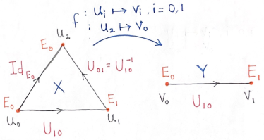
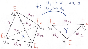
(A)		(B)

Figure 1. (A) Fibers and transports in $X$ are obtained from $Y$ via abstract simplicial map $f:X\to Y$ shown. A transport map in $X$ is identity map when an edge like $[u_{0}u_{2}]$ collapses under $f$. See Definition 3.9 and Example 3.11. (B) Pullback of a 1-cochain $\alpha$ from $Y$ to $X$. The signs for the values in $X$ depend on the assumed orientation in $X$. For example, the value on $[u_{1}u_{3}]$ is $-\alpha_{01}$ since the edge maps to $[v_{1}v_{0}]$. The origin vertices in $X$ are selected from preimages of origin vertices in $Y$. Such pulled back origin vertices are unique for simplices that do not collapse. See Definition 3.13 and Example 3.14.

Let $X$ be the three-dimensional abstract simplicial complex with vertices, $u_{0},u_{1},u_{2},u_{3}$ (tetrahedron) and $Y$ the two-dimensional complex with vertices $v_{0}$, $v_{1}$, $v_{2}$ (triangle), and $(E,\nabla)$ a discrete vector bundle with connection on $Y$. See Figure 1(B). Assume that all the simplices are oriented by increasing vertex index numbers. For example, $[u_{0},u_{2},u_{3}]$ is the positive orientation for that triangle, etc. Let $f:X\to Y$ be the abstract simplicial map with the vertex map $u_{i}\mapsto v_{i}$ for $i=0,1,2$ and $u_{3}\mapsto v_{0}$. Thus $[u_{0},u_{3}]\mapsto v_{0}$, $[u_{1},u_{3}]\mapsto[v_{1},v_{0}]$, $[u_{2},u_{3}]\mapsto[v_{2},v_{0}]$, $[u_{0},u_{1},u_{2}]\mapsto[v_{0},v_{1},v_{2}]$ etc.. The pullback bundle $f^{\ast}E$ on $X$ has fiber $E_{0}$ at vertices $u_{0}$ and $u_{3}$ and fibers $E_{1}$ and $E_{2}$ at $u_{1}$ and $u_{2}$, respectively. Let the origin vertices in $Y$ be the lowest indexed vertices in each simplex, e.g., origin of $[v_{0},v_{1},v_{2}]$ is $v_{0}$, origin of $[v_{1},v_{2}]$ is $v_{1}$ etc. Then the origin vertices for the edges in $X$ can be chosen to be: $u_{0}$ for $[u_{0},u_{1}]$ and $[u_{0},u_{2}]$, $u_{0}$ or $u_{3}$ for $[u_{0},u_{3}]$, $u_{1}$ for $[u_{1},u_{2}]$ and $u_{3}$ for $[u_{1},u_{3}]$ and $[u_{2},u_{3}]$. The origin vertices for the triangles in $X$ can be chosen to be $u_{0}$ for $[u_{0},u_{1},u_{2}]$, $u_{0}$ or $u_{3}$ for $[u_{0},u_{1},u_{3}]$ and $[u_{0},u_{2},u_{3}]$ and $u_{3}$ for $[u_{1},u_{2},u_{3}]$. The origin vertex for the tetrahedron in $X$ can be chosen to be $u_{0}$ or $u_{3}$.

Let $\alpha\in C^{1}(Y;E)$. We compute its pullback to the 1-cochain $f^{\ast}\alpha$ on $X$. For the edges of the triangle $[u_{0},u_{1},u_{2}]$, $\langle f^{\ast}\alpha,[u_{0},u_{1}]\rangle_{u_{0}}=\langle\alpha,f([u_{0},u_{1}])\rangle_{f(u_{0})}=\langle\alpha,[v_{0},v_{1}]\rangle_{v_{0}}$ and similarly for $[u_{0},u_{2}]$ and $[u_{1},u_{2}]$. Since the tetrahedron edge $[u_{0},u_{3}]$ collapses to the vertex $v_{0}$ the pullback to this edge is 0 for dimensional reason, i.e., $\langle f^{\ast}\alpha,[u_{0},u_{3}]\rangle_{u_{0}}=\langle\alpha,f([u_{0},u_{3}])\rangle_{f(u_{0})}=\langle\alpha,[v_{0}]\rangle_{v_{0}}=0$. The same is true if $u_{3}$ is used as the origin vertex for $[u_{0},u_{3}]$. The evaluation of the pullback to the remaining two edges $[u_{1},u_{3}]$ and $[u_{2},u_{3}]$ will involve a sign change. Specifically $\langle f^{\ast}\alpha,[u_{1},u_{3}]\rangle_{u_{3}}=\langle\alpha,f([u_{1},u_{3}])\rangle_{f(u_{3})}=\langle\alpha,[v_{1},v_{0}]\rangle_{v_{0}}=-\langle\alpha,[v_{0},v_{1}]\rangle_{v_{0}}$. Similarly $\langle f^{\ast}\alpha,[u_{2},u_{3}]\rangle_{u_{3}}=\langle\alpha,f([u_{2},u_{3}])\rangle_{f(u_{3})}=-\langle\alpha,[v_{0},v_{2}]\rangle_{v_{0}}$ since the edge $[u_{2},u_{3}]$ of the tetrahedron $X$ maps to the edge $[v_{2},v_{0}]$ of the triangle $Y$.

4. Flat vector bundles and trivializability

Suppose we are given a discrete vector bundle with a choice of gauge, i.e., each fiber is equipped with a choice of basis determining an isomorphism $E_{i}\cong\mathbb{R}^{n}$ or $\mathbb{C}^{n}$. Changing the basis has the effect of conjugating the parallel transport matrices as in (7). In good cases, there are choices of basis in which these parallel transport matrices can be simplified. Most optimistically, one might ask to transform the parallel transport matrices into identity matrices. This is formalized in the notion of a trivialization of a discrete vector bundle with connection, defined as follows.

Definition 4.1.

The rank $n$ trivial real (respectively, complex) discrete vector bundle with connection over $X$ has fiber $\mathbb{R}^{n}$ (respectively, $\mathbb{C}^{n}$) at each vertex, and the identity $\operatorname{Id}_{\mathbb{R}^{n}}$ (respectively $\operatorname{Id}_{\rm\mathbb{C}^{n}}$) parallel transport maps on each edge of $X$. We use the notation $\underline{\mathbb{R}}^{n}$ (respectively, $\underline{\mathbb{C}}^{n}$) to denote the trivial discrete vector bundle with connection. A bundle $(E,\nabla)$ over $X$ is trivializable if it is isomorphic to the trivial bundle. A choice of isomorphism with the trivial bundle is a trivialization. Equivalently, a bundle $(E,\nabla)$ is trivializable if there is a choice of basis for each fiber $E_{i}\cong\mathbb{R}^{n}$ (or $E_{i}\cong\mathbb{C}^{n}$) such that every parallel transport map is the identity matrix.

We will not consider trivializations of discrete vector bundles without connection. Hence, we are interested in discrete analogs of geometric obstructions to trivializability in smooth geometry (namely, curvature) rather than topological ones (e.g., Chern classes).

Curvature of a vector bundle with connection on a smooth manifold can be understood in terms of parallel transport along infinitesimal loops. With this in mind, obstructions to the existence of a trivialization of a discrete vector bundle with connection will be constructed out of parallel transport along loops and paths in the underlying simplicial complex. We therefore start with the following definitions of paths and loops borrowed from graph theory.

Definition 4.2.

A path $\gamma$ in a simplicial complex $X$ is a sequence of vertices $v_{0},\ldots,v_{k}$ such that $[v_{i},v_{i+1}]$ is an edge in $X$, for $i=0,\ldots,k-1$. The edges $[v_{i},v_{i+1}]$ are then called edges of $\gamma$. A loop is a path such that $v_{0}=v_{k}$. The base point of a loop is the vertex $v_{0}$.

Note that vertices and edges of a path may be repeated. That is, a path may self-intersect at vertices and edges.

Definition 4.3.

Given a discrete vector bundle with connection $(E,\nabla)$, the parallel transport along a path $\gamma$ is the composition of the parallel transport maps (adjusted according to edge orientations) encountered along the edges of $\gamma$ in the order they appear. The holonomy $\text{hol}(\gamma)$ of a loop $\gamma$ is the parallel transport along the loop considered as a path from $v_{0}$ to itself.

The following definition is adapted from simple homotopy theory [14].

Definition 4.4.

An elementary simple homotopy of a path $v_{0},\ldots,v_{i}^{\prime},v_{i},v_{i}^{\prime\prime},\dots,v_{k}$ in a simplicial complex $X$ is a path $v_{0},\ldots,v_{i}^{\prime},v_{i}^{\prime\prime},\dots,v_{k}$ where the vertices $v_{i},v_{i}^{\prime},v_{i}^{\prime\prime}$ determine a 2-simplex in $X$. Two paths are simply homotopic if one can be obtained from the other by a finite sequence of elementary simply homotopies that leave the endpoints fixed.

Definition 4.5.

A discrete vector bundle with connection is flat (or the connection is flat) if the parallel transport between any two points only depends on the simple homotopy class of the path connecting the two points.

Later we shall give an equivalent characterization in terms of vanishing curvature, see Proposition 8.5. The flatness property defined above is straightforward to check for a given discrete vector bundle with connection using the following result.

Lemma 4.6.

A connection is flat if and only if holonomy around every 2-simplex is the identity.

Proof.

If the holonomy around every 2-simplex is the identity, then parallel transport is invariant under elementary simple homotopies. Hence, parallel transport only depends on the simple homotopy class of the path. The converse is obvious. ∎

For the remainder of this section we will assume that $X$ is connected; this implies the existence of a spanning tree in the 1-skeleton $X^{(1)}$ of $X$.

Lemma 4.7.

Given a vector bundle $(E,\nabla)$ over a connected simplicial complex $X$, its restriction over any spanning tree of $X^{(1)}$ is trivializable.

Proof.

Fix a spanning tree $T$ of $X^{(1)}$. Choose a basis for the fiber $E_{0}$ at the root $0$ of $T$. Then for every other vertex $i$ of $X$ take the unique basis of $E_{i}$ determined by the parallel transport of the basis of $E_{0}$ to $E_{i}$. The uniqueness of this parallel transport map follows from the uniqueness of paths between vertices of a tree. The resulting bases provide isomorphisms from $E_{i}$ to $\mathbb{R}^{n}$ for each $k$. Furthermore, the parallel transport matrices in this choice of gauge are identity matrices by construction. ∎

Definition 4.8.

The fundamental group $\pi_{1}(X,0)$ of a simplicial complex $X$ with respect to a base vertex $0$ is the set of loops in $X$ based at $0$ modulo the equivalence relation of simply homotopy. This set is endowed with a group structure inherited from concatenation of loops.

Given a flat discrete vector bundle with connection $(E,\nabla)$ over a connected simplicial complex $X$ with a chosen basepoint $0$, consider the map of sets

(8) $$\rho\colon\pi_{1}(X,0)\to{\rm GL}(E_{0})\qquad[\gamma]\mapsto\text{hol}(\gamma).$$

Lemma 4.9.

The map (8) is a homomorphism of groups. For basepoints $0$ and $0^{\prime}$, we obtain homomorphisms $\rho\colon\pi_{1}(X,0)\to{\rm GL}(E_{0})$ and $\rho^{\prime}\colon\pi_{1}(X,0^{\prime})\to{\rm GL}(E_{0^{\prime}})$ that are compatible via isomorphisms $\pi_{1}(X,0)\to\pi_{1}(X,0^{\prime})$ and ${\rm GL}(E_{0})\to{\rm GL}(E_{0^{\prime}})$ uniquely specified by a homotopy class of path joining $0$ and $0^{\prime}$.

Proof.

First we observe that the map is well-defined because the discrete vector bundle with connection is assumed to be flat. Next, we recall that the group structure on $\pi_{1}(X,0)$ comes from concatenation of loops, $(\gamma,\gamma^{\prime})\mapsto\gamma*\gamma^{\prime}$. From the definition of holonomy as a composition of parallel transport matrices, it is immediate that $\text{hol}(\gamma*\gamma^{\prime})=\text{hol}(\gamma)\circ\text{hol}(\gamma^{\prime})$ and the first statement follows. If $0$ and $0^{\prime}$ are different choices of basepoint a choice of path from $0$ to $0^{\prime}$ determines a change-of-basepoint isomorphism $\pi_{1}(X,0)\to\pi_{1}(X,0^{\prime})$ gotten by pre- and post-composing a loop based at $0$ with the path from $0$ to $0^{\prime}$. By construction, this isomorphism only depends on the homotopy class of the path. Parallel transport along the path from $0$ to $0^{\prime}$ gives an isomorphism ${\rm GL}(E_{0})\to{\rm GL}(E_{0^{\prime}})$. Flatness of the connection guarantees that this isomorphism only depends on the homotopy class of the path. ∎

We have the following trivializability result.

Proposition 4.10.

A discrete vector bundle with connection $(E,\nabla)$ over a connected simplicial complex $X$ is trivializable if and only if (i) $(E,\nabla)$ is flat, and (ii) the homomorphism (8) is trivial for one (and hence any) choice of basepoint.

Proof.

For ease of notation, we treat the case of a real vector bundle; the complex case is identical. Suppose $(E,\nabla)$ is trivializable. Choose a trivialization whose data are specified by isomorphisms $\varphi_{i}:E_{i}\to\mathbb{R}^{n}$ for each vertex. Then relative to these choices of basis, the parallel transport matrices are identity matrices. Then it is clear that the holonomy around any loop $\gamma$ (not just homotopically trivial one) is the identity map for any choice of basepoint. This proves the forward implication. Conversely, suppose conditions (i) and (ii) are satisfied. Then choose a spanning tree $T$ of $X^{(1)}$ rooted at vertex 0 and trivialize according to Lemma 4.7. Note that this trivialization fixes an isomorphism $\varphi_{i}:E_{i}\to\mathbb{R}^{n}$ and hence a basis of $E_{i}$ for each vertex $i$. Now let $e$ be an edge not in $T$ and $\gamma$ be a loop containing $e$ such that every other edge in $\gamma$ is in $T$. Since the parallel transport matrices on $T$ are identities and (8) is assumed to be the trivial homomorphism, $U_{e}$ is also the identity matrix. This completes the proof. ∎

A connected simplicial complex $X$ is simply connected if $\pi_{1}(X,0)=\{e\}$. The following corollary to Proposition 4.10 shows that flatness completely determines trivializability in the simply connected case.

Corollary 4.11.

Given a discrete vector bundle with connection $(E,\nabla)$ over a simply connected simplicial complex $X$, then $(E,\nabla)$ is trivializable if and only if $(E,\nabla)$ is flat.

5. Reduction of structure group and trivial subbundles

The following definition will allow us to consider intermediate versions of trivializability of a discrete vector bundle with connection.

Definition 5.1.

Let $G$ be a subgroup of ${\rm GL}_{n}(\mathbb{R})$ (respectively, ${\rm GL}_{n}(\mathbb{C})$). A real discrete vector bundle with connection $(E,\nabla)$ has structure group $G$ if the fibers $E_{i}$ of $E$ are all the vector space $\mathbb{R}^{n}$ (respectively $\mathbb{C}^{n}$) and the parallel transport matrices are elements of $G$. A discrete vector bundle with connection has reduction to structure group $G$ if it is isomorphic to a discrete vector bundle with structure group $G$.

Example 5.2.

For a discrete vector bundle with connection $(E,\nabla)$, reduction of structure group to the trivial group $\{e\}<{\rm GL}_{n}$ is equivalent to a choice of trivialization.

Example 5.3.

Recall Definition 3.8 of the Whitney sum of discrete vector bundles with connection. Given a rank $n$ discrete vector bundle with connection, there exists a rank $k$ discrete vector bundle with connection $(E^{\prime},\nabla^{\prime})$, a rank $(n-k)$ discrete vector bundle with connection $(E^{\prime\prime},\nabla^{\prime\prime})$ and an isomorphism $(E,\nabla)\cong(E^{\prime},\nabla^{\prime})\oplus(E^{\prime\prime},\nabla^{\prime\prime})$ if and only if there is a reduction to block diagonal structure group,

(9) $$G:=\left\{\left[\begin{array}[]{cc}A&0\\ 0&B\end{array}\right]\in{\rm GL}_{n}\mid A\in{\rm GL}_{k},B\in{\rm GL}_{n-k}\right\}\,.$$

Example 5.4.

Suppose that the fibers of a discrete vector bundle with connection are equipped with the structure of inner product spaces. Then parallel transport maps preserve the inner products if and only if there exists a reduction of structure group to ${\rm O}(n)<{\rm GL}_{n}(\mathbb{R})$. Similar remarks apply in the complex case for Hermitian forms and reduction to the unitary group, ${\rm U}(n)<{\rm GL}_{n}(\mathbb{C})$.

The above example prompts the following definition; we will return to this in more detail at the end of §7.

Definition 5.5.

Let $(E,\nabla)$ be a discrete vector bundle with connection. A metric on $E$ is the structure of an inner product space on each vector space $E_{i}$. The connection $\nabla$ is metric compatible if the parallel transport matrices $U_{ji}$ are inner product preserving linear maps for every edge $[ij]$. Equivalently, a connection is metric compatible if it has structure group ${\rm O}(n)<{\rm GL}_{n}(\mathbb{R})$, the orthogonal group.

Special cases of reduction of structure group recover classical problems in linear algebra.

Example 5.6.

Consider the discrete vector bundle with connection on a triangle $[012]$ from Example 3.7 with parallel transport matrices $A=U_{10}$ and identity matrices $I=U_{21}=U_{20}$ for the other edges. Gauge transformations $g_{i}=P$ that are equal at all vertices then have the effect

$$U_{10}=A\mapsto P^{-1}AP,\quad U_{21}=U_{20}=I\mapsto PIP^{-1}=I.$$

Hence in this example, questions about the reduction of structure group amount to similarity transformations for the matrix $A$. Explicitly, for a subgroup $G<{\rm GL}_{n}$, we ask whether there exists $B\in G$ and $P\in{\rm GL}_{n}$ with $P^{-1}AP=B$.

Definition 5.7.

Given a discrete vector bundle with connection $(E,\nabla)$ over a simplicial complex $X$ a subbundle is a discrete vector bundle with connection $(E^{\prime},\nabla^{\prime})$ over $X$ and a map of discrete vector bundles $(E^{\prime},\nabla^{\prime})\to(E,\nabla)$ over $\operatorname{Id}_{X}$ whose maps on fibers are inclusion of subspaces $E_{i}^{\prime}\subset E_{i}$ for each vertex $i\in X^{(0)}$. We use the notation $(E^{\prime},\nabla^{\prime})\subset(E,\nabla)$ to denote a subbundle.

Note that the definition of a map of discrete vector bundles with connection requires the parallel transport matrices for a subbundle to satisfy $U_{ji}|_{E_{i}^{\prime}}(E_{i}^{\prime})\subseteq E_{j}^{\prime}\subset E_{j}$ for all edges $[ij]\in X^{(1)}$.

Definition 5.8.

Arank $k$ trivial subbundle of a discrete vector bundle with connection is a subbundle $(E^{\prime},\nabla^{\prime})\subset(E,\nabla)$ and an isomorphism from $(E^{\prime},\nabla^{\prime})$ to $\underline{\mathbb{R}}^{k}$, the trivial rank $k$ discrete vector bundle with connection (or $\underline{\mathbb{C}}^{k}$ in the complex case).

An intermediate question to trivializability of a discrete vector bundle with connection is the following. Given a discrete vector bundle with connection $(E,\nabla)$ what is the largest $k$ for $(E,\nabla)$ has a rank $k$ trivial subbundle?

Proposition 5.9.

A discrete vector bundle with connection $(E,\nabla)$ has a rank $k$ trivial subbundle if and only if it admits a reduction of structure group to the subgroup of block upper-triangular matrices of the form

(10) $$G:=\left\{\left[\begin{array}[]{cc}\operatorname{Id}_{k}&*\\ 0&A\end{array}\right]\in{\rm GL}_{n}\mid A\in{\rm GL}_{n-k}\right\}\,$$

where $*$ is an arbitrary $k\times(n-k)$ matrix.

Proof.

If the reduction of structure group exists, then the block upper-triangular form of $G$ yields an evident rank $k$ trivial subbundle given by the inclusions $\mathbb{R}^{k}\subset\mathbb{R}^{n}$. Conversely, suppose that $(E,\nabla)$ has a rank $k$ trivial subbundle. This gives the data of an injection $\mathbb{R}^{k}\hookrightarrow E_{i}$ for each fiber $E_{i}$, where the first $k$ basis vectors are the previously chosen basis for the image of $\mathbb{R}^{k}\hookrightarrow E_{i}$. Extend the image of the basis vector of $\mathbb{R}^{k}$ in $E_{i}$ to a basis of $E_{i}$ for each $i$. In this choice of gauge, the parallel transport matrices then take the form (10). ∎

Definition 5.10.

A section $s$ of a discrete vector bundle with connection is parallel if $\nabla s=0$. A set of parallel sections $\{s^{1},s^{2},\dots,s^{k}\}$ is linearly independent if the restriction to each fiber $E_{v}$ gives a linearly independent set $\{s^{1}_{v},s^{2}_{v},\dots,s^{k}_{v}\}$.

Corollary 5.11.

A discrete vector bundle with connection $(E,\nabla)$ admits a rank $k$ trivial subbundle if and only if there exists a set of $k$ linearly independent parallel sections.

Proof.

Extend the linearly independent set $\{s^{1}_{v},s^{2}_{v},\dots,s^{k}_{v}\}$ at each $E_{v}$ to a basis. In this choice of gauge, parallel transport matrices take the form (10) and the result follows. ∎

6. Wedge Product and Naturality

We define a combinatorial wedge product between vector bundle valued and scalar valued cochains by a cup product. In contrast, the combinatorial wedge product for scalar valued cochains in DEC incorporates an anti-symmetrization of the cup product [22]. This difference is due to a curvature obstruction that arises in the discrete vector bundle case. This will be elaborated upon in §9. We show that the combinatorial wedge product is natural with respect to pullbacks under simplicial maps of the base simplicial complex. The anti-commutativity result follows from the corresponding cup product result for scalar-valued cochains. As in DEC, the wedge product is not associative. Just as the lack of associativity of the discrete wedge product is related to $A_{\infty}$-algebras, we expect the curvature obstruction to Leibniz rule in the presence of anti-symmetrization to lead to algebraic structures that may turn out to be interesting on their own.

As mentioned in Remark 3.4 all constructions including the ones in this section will first be done assuming a total ordering on vertices of $X$. This restriction will be removed starting from §10.

In §7 we define a discrete exterior covariant derivative $d_{\nabla}$ and show that the discrete wedge product satisfies the Leibniz rule with respect to $d_{\nabla}$.

Definition 6.1.

Given a vector bundle valued cochain $\alpha\in C^{k}(X;E)$ and scalar-valued cochain $w\in C^{l}(X)$ their wedge product $\alpha\wedge w$ is defined by its evaluation on a $(k+l)$-simplex at the origin vertex as

(11) $$\langle\alpha\wedge w,[0\,...\,k+l]\rangle_{0}:=\langle\alpha\smile w,[0\,...\,k+l]\rangle_{0}=\langle\alpha,[0\,...\,k]\rangle_{0}\,\langle w,[k\,...\,k+l]\rangle$$

Remark 6.2.

To ensure that $\alpha\wedge w$ is a cochain the LHS of (11) should change sign according to the permutation of the simplex it is evaluated on. This is achieved by requiring that if $\tau\in S_{k+l+1}$ is a permutation and the LHS is evaluated on $[\tau(0),\ldots,\tau(k+l)]$ then

$$\langle\alpha\wedge w,[\tau(0),\ldots,\tau(k+l)]\rangle_{0}:=\operatorname{sgn}(\tau)\langle\alpha\wedge w,[0\,...\,k+l]\rangle_{0}=\operatorname{sgn}(\tau)\langle\alpha,[0\,...\,k]\rangle_{0}\;\langle w,[k\,...\,k+l]\rangle\,.$$

From the definition of the cup product and pullbacks one has the following naturality result.

Proposition 6.3 (Naturality of wedge product).

Let $X,Y$ be simplicial complexes, $(E,\nabla)$ a discrete vector bundle with connection over $Y$ and $f:X\to Y$ an abstract simplicial map. Then for any $\alpha\in C^{k}(Y;E)$ and $w\in C^{l}(Y)$ and simplex $[u_{0}\,...\,u_{k+l}]$ in $X$ with origin vertex $u_{0}$

(12) $$\langle f^{\ast}(\alpha\wedge w),[u_{0}\,...\,u_{k+l}]\rangle_{u_{0}}=\langle f^{\ast}\alpha\wedge f^{\ast}w,[u_{0}\,...\,u_{k+l}]\rangle_{u_{0}}$$

Proof.

Since the wedge product is defined using the cup product this naturality property follows from the definitions since

$$\langle f^{\ast}(\alpha\smile w),[u_{0}\,...\,u_{k+l}]\rangle_{u_{0}} =\langle\alpha\smile w,f([u_{0}\,...\,u_{k+l}])\rangle_{f(u_{0})}=\langle\alpha\smile w,[f(u_{0})\,...\,f(u_{k+l})]\rangle_{f(u_{0})}$$

$$=\langle\alpha,[f(u_{0})\,...\,f(u_{k})]\rangle_{f(u_{0})}\;\;\langle w,[f(u_{k})\,...\,f(u_{k+l})]\rangle$$

$$=\langle f^{\ast}\alpha,[u_{0}\,...\,u_{k}]\rangle_{u_{0}}\langle f^{\ast}w,[u_{k}\,...\,u_{k+l}]\rangle$$

$$=\langle f^{\ast}\alpha\smile f^{\ast}w,[u_{0}\,...\,u_{k+l}]\rangle_{u_{0}}\,.$$

For dimensional reasons, both sides are 0 if the vertex map of $f$ is not a bijection. ∎

7. Discrete exterior covariant derivative

The covariant derivative $\nabla$ in smooth geometry is initially defined as an an operator on sections of a smooth vector bundle. It has a natural extension to the exterior covariant derivative $d_{\nabla}$, an operator on vector bundle valued differential forms as in (2). This extension has important geometric content, e.g., $d_{\nabla}$ squares to the curvature of the connection.

Similarly, the discrete covariant derivative was initially defined as an operator on sections in Definition 3.5. In this section we extend it to vector bundle valued $k$-cochains for $k>0$. This generalization is the simplicial interpretation of the operator defined in infinitesimal context by Kock [27]. We show here that this simplicial interpretation satisfies Leibniz rule with respect to the discrete wedge product defined in §6 and it commutes with pullback by abstract simplicial maps.

As above, throughout this section $(E,\nabla)$ denotes a discrete vector bundle with connection over a simplicial complex $X$.

Definition 7.1.

Let $\alpha\in C^{k-1}(X;E)$ be a $(k-1)$-cochain. The discrete exterior covariant derivative of $\alpha$ is the $k$-cochain $d_{\nabla}\alpha\in C^{k}(X;E)$ defined by

(13) $$\langle d_{\nabla}\alpha,[0\,...\,k]\rangle_{0}\mathrel{\mathop{:}}=U_{01}\langle\alpha,[1\,...\,k]\rangle_{1}+\sum_{i=1}^{k}(-1)^{i}\langle\alpha,[0\,...\,\hat{i}\,...\,k]\rangle_{0}\,$$

for $\sigma=[0\,...\,k]$ a $k$-simplex in $X$.

As mentioned in §3 Leibniz rule is a defining property of covariant derivative and expresses compatibility of the exterior covariant derivative with the de Rham differential. This is also the case for the exterior covariant derivative. We first prove this for sections and then extend it to higher degree cochains.

Proposition 7.2 (Leibniz rule for sections).

For any $f\in C^{0}(X)$, section $s\in C^{0}(X;E)$ and edge $[ij]$ in $X$ with origin vertex $i$:

(14) $$\langle\nabla(f\wedge s),[ij]\rangle_{i}=\langle df\wedge s+f\wedge\nabla s,[ij]\rangle_{i}\,.$$

Proof.

The LHS is $U_{ij}(f_{j}s_{j})-f_{i}s_{i}$. On the RHS

$$\langle df\wedge s,[ij]\rangle_{i} =\langle df,[ij]\rangle U_{ij}s_{j}=(f_{j}-f_{i})U_{ij}s_{j}$$

$$\langle f\wedge\nabla s,[ij]\rangle_{i} =f_{i}\langle\nabla s,[ij]\rangle_{i}=f_{i}(U_{ij}s_{j}-s_{i})\,.$$

Thus

$$\langle df\wedge s,[ij]\rangle_{i}+\langle f\wedge\nabla s,[ij]\rangle_{i} =(f_{j}-f_{i})U_{ij}s_{j}+f_{i}(U_{ij}s_{j}-s_{i})$$

$$=U_{ij}(f_{j}s_{j})-f_{i}s_{i}\,.$$

∎

Proposition 7.3 (Leibniz rule).

The operators $d_{\nabla}$ and $d$ satisfy a Leibniz rule with respect to the wedge product of $\alpha\in C^{k}(X;E)$ and $w\in C^{l}(X)$. That is:

(15) $$\langle d_{\nabla}(\alpha\wedge w),[0\,...\,k{+}l{+}1]\rangle_{0}=\langle d_{\nabla}\alpha\wedge w,[0\,...\,k{+}l{+}1]\rangle_{0}+(-1)^{k}\langle\alpha\wedge dw,[0\,...\,k{+}l{+}1]\rangle_{0}$$

Proof.

Since the discrete wedge product for identity permutation is just the cup product the proof is written using the latter. By definition of $d_{\nabla}$, the LHS of (15) is

$$U_{01}\langle\alpha\smile w,[1\,...\,k{+}l{+}1]\rangle_{1}+\sum_{i=1}^{k{+}l{+}1}(-1)^{i}\langle\alpha\smile w,[0\,...\,\hat{i}\,...\,k{+}l{+}1]\rangle_{0}\,.$$

Next we evaluate the cup products. The summation above is split into two so that the omitted index is either in the evaluation of $\alpha$ or in the evaluation of $w$. Thus the LHS of (15) becomes:

(16) $$U_{01}\langle\alpha,[1\,...\,k+1]\rangle_{1}\;\langle w,[k{+}1\,...\,k{+}l{+}1]\rangle+\sum_{i=1}^{k}(-1)^{i}\langle\alpha,[0\,...\,\hat{i}\,...\,k{+}1]\rangle_{0}\;\langle w,[k{+}1\,...\,k{+}l{+}1]\rangle+\\ \sum_{i=k{+}1}^{k{+}l{+}1}(-1)^{i}\langle\alpha,[0\,...\,k]\rangle_{0}\;\langle w,[k\,...\,\hat{i}\,...\,k{+}l{+}1]\rangle\,.$$

The first term on the RHS of (15) is

$$\langle d_{\nabla}\alpha,[0\,...\,k+1]\rangle_{0}\;\langle w,[k+1\,...\,k{+}l{+}1]\rangle\,,$$

which expands to

$$U_{01}\langle\alpha,[1\,...\,k{+}1]\rangle_{1}\;\langle w,[k+1\,...\,k{+}l{+}1]\rangle+\sum_{i=1}^{k+1}(-1)^{i}\langle\alpha,[0\,...\,\hat{i}\,...\,k{+}1]\rangle_{0}\;\langle w,[k{+}1\,...\,k{+}l{+}1]\rangle\,.$$

In preparation for a cancellation we will separate out the last term in the summation above, which yields

(17) $$U_{01}\langle\alpha,[1\,...\,k{+}1]\rangle_{1}\;\langle w,[k{+}1\,...\,k{+}l{+}1]\rangle\;+\\ \sum_{i=1}^{k}(-1)^{i}\langle\alpha,[0\,...\,\hat{i}\,...\,k{+}1]\rangle_{0}\;\langle w,[k{+}1\,...\,k{+}l{+}1]\rangle+(-1)^{k+1}\langle\alpha,[0\,...\,k]\rangle_{0}\;\langle w,[k{+}1\,...\,k{+}l{+}1]\rangle\,.$$

The second term of the RHS of (15) with the sign $(-1)^{k}$ included evaluates to

$$(-1)^{k}\langle\alpha,[0\,...\,k]\rangle_{0}\;\langle dw,[k\,...\,k{+}l{+}1]\rangle=(-1)^{k}\langle\alpha,[0\,...\,k]\rangle_{0}\;\sum_{i=k}^{k+l+1}(-1)^{(i-k)}\langle w,[k\,...\,\hat{i}\,...\,k{+}l{+}1]\rangle\,.$$

Separating out the first term in the summation above yields

(18) $$(-1)^{k}\langle\alpha,[0\,...\,k]\rangle_{0}\;(-1)^{0}\langle w,[k{+}1\,...\,k{+}l{+}1]\rangle+\\ (-1)^{k}\sum_{i=k+1}^{k+l+1}\langle\alpha,[0\,...\,k]\rangle_{0}\;(-1)^{(i-k)}\langle w,[k\,...\,\hat{i}\,...\,k{+}l{+}1]\rangle\,.$$

On adding (17) and (18) the last term in (17) and the first term in (18) cancel and the result is  (16). ∎

The fact that the exterior derivative for de Rham complex commutes with pullback by smooth maps is the generalization of chain rule of calculus. Such a naturality property is satisfied by the discrete exterior covariant derivative, with smooth maps replaced by abstract simplicial maps.

Proposition 7.4 (Naturality of $d_{\nabla}$).

Let $(E,\nabla)$ be a discrete vector bundle with connection on a simplicial complex $Y$, and $f:X\to Y$ an abstract simplicial map. Then for any $\alpha\in C^{k}(Y;E)$ and $(k+1)$-simplex $[u_{0}\,...\,u_{k+1}]$ in $X$ with origin vertex $u_{0}$:

(19) $$\langle f^{\ast}d_{\nabla}\alpha,[u_{0}\,...\,u_{k+1}]\rangle_{u_{0}}=\langle d_{\nabla}f^{\ast}\alpha,[u_{0}\,...\,u_{k+1}]\rangle_{u_{0}}\,.$$

Proof.

Let $f([u_{0}\,...\,u_{k+1}])$ be an $l$-simplex in $Y$. There are two cases to consider: $l=k+1$ or $l<k+1$. For the case of $l=k+1$, (19) follows in a straightforward manner from definitions of the discrete pullback bundle and discrete exterior covariant derivative. The case $l<k+1$ arises when at least two of the vertices of $[u_{0}\,...\,u_{k+1}]$ map to the same vertex in $Y$. Since vertex labels are arbitrary, suppose without loss of generality that $f(u_{0})=f(u_{1})=v_{0}$. There may be other vertices that map to a common vertex, but it is enough to consider just one pair. The LHS of (19) is then 0. In the pullback bundle $f^{\ast}E$ over $X$ the parallel transport map on the edge $[u_{0},u_{1}]$ is $\operatorname{Id}_{E_{0}}$ where $E_{0}$ is the fiber over vertex $v_{0}$ in $Y$. Thus RHS of (19) is

$$\langle\alpha,f([u_{1}\,...\,u_{k+1}])\rangle_{u_{1}}+\sum_{j=1}^{k+1}(-1)^{j}\langle\alpha,f([u_{0}\,...\,\widehat{u_{j}}\,...\,u_{k+1}])\rangle_{u_{0}}\,.$$

If $l<k$ then each term in the above expression is 0. If $l=k$ then the above expression reduces to

$$\langle\alpha,f([u_{1}\,...\,u_{k+1}])\rangle_{u_{1}}-\langle\alpha,f([u_{0}\widehat{u_{1}}\,...\,u_{k+1}])\rangle_{u_{0}}\,,$$

which is 0 since $f(u_{0})=f(u_{1})$ and the transport map from $u_{1}$ to $u_{0}$ is identity. ∎

Corollary 7.5.

Given simplicial complexes $X$ and $Y$, abstract simplicial map $f:X\to Y$ and a scalar-valued cochain $\alpha\in C^{k}(Y)$, pullback by $f$ commutes with the discrete exterior derivative, that is, $f^{\ast}d=d\;f^{\ast}$.

Proof.

This follows by noting that the definition of the discrete exterior derivative $d$ is the same as that for $d_{\nabla}$ when $U_{01}=\operatorname{Id}_{E_{0}}$ and the rank of the bundle over $X$ is 1. ∎

Example 7.6.

Let $X$, $Y$, $(E,\nabla)$, $f:X\to Y$ and $\alpha\in C^{1}(Y;E)$ be as in Example 3.14. We will check that $\langle d_{\nabla}f^{\ast}\alpha,[u_{i},u_{j},u_{k}]\rangle_{u}=\langle f^{\ast}d_{\nabla}\alpha,[u_{i},u_{j},u_{k}]\rangle_{u}$ for all triangles $[u_{i},u_{j},u_{k}]$ of $X$, where $u$ is a pulled back origin vertex in $[u_{i},u_{j},u_{k}]$. For $Y$ let the origin vertices be the lowest indexed vertices in each simplex. For $f^{\ast}E$, the origin vertices are pulled back from $E$ on $Y$.

The transport maps of the pullback bundle $f^{\ast}E$ over $X$ are $U_{10},U_{20}$ and $U_{21}$ on edges $[u_{0},u_{1}]$, $[u_{0},u_{2}]$ and $[u_{1},u_{2}]$, respectively. On the other three edges of $X$ the transport maps are $\operatorname{Id}_{E_{0}}$ on $[u_{0},u_{3}]$, $U_{01}=U_{10}^{-1}$ on $[u_{1},u_{3}]$ and $U_{02}=U_{20}^{-1}$ on $[u_{2},u_{3}]$. Now we compute, using the evaluations of the pullback from Example 3.14. On $[u_{0},u_{1},u_{2}]$ the pulled back origin vertex is $u_{0}$ and

$$\langle d_{\nabla}f^{\ast}\alpha,[u_{0},u_{1},u_{2}]\rangle_{u_{0}} =U_{01}\langle f^{\ast}\alpha,[u_{1},u_{2}]\rangle_{u_{1}}-\langle f^{\ast}\alpha,[u_{0},u_{2}]\rangle_{u_{0}}+\langle f^{\ast}\alpha,[u_{0},u_{1}]\rangle_{u_{0}}$$

$$=U_{01}\langle\alpha,[v_{1},v_{2}]\rangle_{v_{1}}-\langle\alpha,[v_{0},v_{2}]\rangle_{v_{0}}+\langle\alpha,[v_{0},v_{1}]\rangle_{v_{0}}$$

$$=\langle d_{\nabla}\alpha,[v_{0},v_{1},v_{2}]\rangle_{v_{0}}=\langle f^{\ast}d_{\nabla}\alpha,[u_{0},u_{1},u_{2}]\rangle_{u_{0}}\,.$$

The origin vertex of $[u_{1},u_{2},u_{3}]$ resulting from the pullback is $u_{3}$ since $f([u_{1},u_{2},u_{3}])=[v_{1},v_{2},v_{0}]$ whose origin is $v_{0}=f(u_{3})$. On this simplex the LHS is

$$\langle d_{\nabla}f^{\ast}\alpha,[u_{1},u_{2},u_{3}]\rangle_{u_{3}}=\langle f^{\ast}\alpha,[u_{2},u_{3}]\rangle_{u_{3}}-\langle f^{\ast}\alpha,[u_{1},u_{3}]\rangle_{u_{3}}+U_{01}\langle f^{\ast}\alpha,[u_{1},u_{2}]\rangle_{u_{1}}\,.$$

Note that the pulled back origin vertex for $[u_{2},u_{3}]$ is $u_{3}$ since $f([u_{2},u_{3}])$ is $[v_{2},v_{0}]$ whose origin vertex is $v_{0}$. The transport map used above is $U_{01}$ since $f^{\ast}E$ has that map associated with the edge $[u_{1},u_{3}]$. Thus the LHS is

$$\langle\alpha,[v_{2},v_{0}]\rangle_{v_{0}}-\langle\alpha,[v_{1},v_{0}]\rangle_{v_{0}}+U_{01}\langle\alpha,[v_{1},v_{2}]\rangle_{v_{1}}\,,$$

Which equals the RHS $\langle d_{\nabla}\alpha,[v_{1},v_{2},v_{0}]\rangle_{v_{0}}$. On $[u_{0},u_{1},u_{3}]$ the pulled back origin vertex is $u_{0}$ and

$$\langle d_{\nabla}f^{\ast}\alpha,[u_{0},u_{1},u_{3}]\rangle_{u_{0}} =\langle f^{\ast}\alpha,[u_{1},u_{3}]\rangle_{u_{3}}-\langle f^{\ast}\alpha,[u_{0},u_{3}]\rangle_{u_{0}}+\langle f^{\ast}\alpha,[u_{0},u_{1}]\rangle_{u_{0}}$$

$$=\langle\alpha,[v_{1},v_{0}]\rangle_{v_{1}}-0+\langle\alpha,[v_{0},v_{1}]\rangle_{v_{0}}$$

$$=0\,.$$

Finally, on the remaining simplex $[u_{0},u_{2},u_{3}]$ we can use either $u_{0}$ or $u_{3}$ as the pulled back origin vertex since this triangle collapses on to the edge $[v_{0},v_{2}]$ whose origin is $v_{0}$ to which both $u_{0}$ and $u_{3}$ map. Using $u_{0}$ as the origin,

$$\langle d_{\nabla}f^{\ast}\alpha,[u_{0},u_{2},u_{3}]\rangle_{u_{0}} =\langle f^{\ast}\alpha,[u_{2},u_{3}]\rangle_{u_{3}}-\langle f^{\ast}\alpha,[u_{0},u_{3}]\rangle_{u_{0}}+\langle f^{\ast}\alpha,[u_{0},u_{2}]\rangle_{u_{0}}$$

$$=\langle\alpha,[v_{2},v_{0}]\rangle_{v_{0}}-0+\langle\alpha,[v_{0},v_{2}]\rangle_{v_{0}}=0\,,$$

which equals the RHS $\langle f^{\ast}d_{\nabla}\alpha,[u_{0},u_{2},u_{3}]\rangle_{u_{0}}$ which is $\langle d_{\nabla}\alpha,[v_{0},v_{2}]\rangle_{v_{0}}=0$.

Metric compatible connections

Suppose that the fibers of a smooth vector bundle $E\to M$ are equipped with a smoothly-varying inner product $\langle-,-\rangle$. Then a connection $\nabla$ on $E$ is metric compatible if there is an equality of 1-forms,

(20) $$d\langle s,s^{\prime}\rangle=\langle\nabla s,s^{\prime}\rangle+\langle s,\nabla s^{\prime}\rangle\in\Lambda^{1}(M)$$

using the inner product of vector bundle valued forms determined by the inner product on fibers discussed in the next paragraph. One consequence of metric compatibility in the smooth case is that parallel transport with respect to $\nabla$ yields an inner product preserving map on the fibers of $E$. This characterization in terms of parallel transport fits nicely in the discrete framework, as already seen in Definition 5.5. We now seek to show that this previous definition is equivalent to an appropriate discretization of the formula (20).

Before turning to this discrete theory, we recall a construction of the inner product on smooth forms used in (20). Let $\alpha\in\Lambda^{k}(M;E)$ and $\beta\in\Lambda^{l}(M;E)$ for a smooth vector bundle $\pi:E\to M$ of rank $r$. Let $x^{i}$, $i=1,\ldots,n$ be coordinates of $M$ in a coordinate domain $U$ containing $p\in M$ and let $v^{s}$, $s=1,\ldots,r$ be a local frame of $E$ in an open subset of $\pi^{-1}(U)$. In local coordinates, $\alpha=\alpha_{Is}\,dx^{I}\otimes v^{s}$ and $\beta=\beta_{Jt}\,dx^{J}\otimes v^{t}$ where we have used the multi-index notation [29, Chapter 14]. Then $\alpha\wedge\beta$ is a vector bundle valued form in the vector bundle $E\otimes E$ and in local coordinates

$$\alpha\wedge\beta=\alpha_{Is}\beta_{Jt}\,dx^{I}\wedge dx^{J}\otimes v^{s}\otimes v^{t}\,$$

using the Einstein summation notation. Suppose the fibers of $E$ come equipped with an inner product $\langle-,-\rangle$. Then we have the local definition,

(21) $$\langle\alpha,\beta\rangle:=\alpha_{Is}\beta_{Jt}\,dx^{I}\wedge dx^{J}\langle v^{s},v^{t}\rangle\in\Lambda^{k+l}(M)$$

of the inner product as a $(k+l)$-form on $M$.

The above discussion carries over neatly to the discrete case, leading to formula for metric compatible connections as in (20). We start with the definition.

Given a discrete vector bundle with connection $(E,\nabla)$ with metric (as in Definition 5.5), let $u\cdot v$ denote the inner product for $u,v\in E_{i}$. The formula (21) together with the averaging interpretation of wedge products of scalar cochains leads to the correct discrete definition of the inner product on vector bundle valued discrete cochains. We only require the following special cases for 0- and 1-cochains.

Definition 7.7.

Given $\alpha\in C^{1}(X;E)$ and $s,s^{\prime}\in C^{0}(X;E)$ the inner product $\alpha\cdot s\in C^{1}(X)$ of the 1-cochain and section is defined as

$$\langle\alpha\cdot s,[01]\rangle_{0}=\langle s\cdot\alpha,[01]\rangle_{0}\mathrel{\mathop{:}}=\langle\alpha,[01]\rangle_{0}\cdot\frac{s_{0}+U_{01}s_{1}}{2}\,.$$

The inner product between the sections $s$ and $s^{\prime}$ is $s\cdot s^{\prime}\in C^{0}(X)$ and its value at a vertex $0$ is $s_{0}\cdot s^{\prime}_{0}$.

The use of the average value for the section is consistent with the DEC interpretation of a wedge product of a 1-cochain and a 0-cochain.

Proposition 7.8 (Metric compatibility).

Let $(E,\nabla)$ be a discrete vector bundle with metric. Then the connection is metric compatible if and only if for all $s,s^{\prime}\in C^{0}(X;E)$,

(22) $$d(s\cdot s^{\prime})=\nabla s\cdot s^{\prime}+s\cdot\nabla s^{\prime}.$$

i.e., the discrete version of (20) holds.

Proof.

We will only prove the real case, so that the parallel transport maps are assumed to be orthogonal. Let $[01]$ be an edge in $X$. Then the evaluation of the LHS on the edge is $\langle d(s\cdot s^{\prime}),[01]\rangle$ is $s_{1}\cdot s^{\prime}_{1}$ - $s_{0}\cdot s^{\prime}_{0}$. Evaluating the RHS on this edge

$$\langle\nabla s\cdot s^{\prime},[01]\rangle_{0}+\langle s\cdot\nabla s^{\prime},[01]\rangle_{0}=\langle\nabla s,[01]\rangle_{0}\cdot\frac{s^{\prime}_{0}+U_{01}s^{\prime}_{1}}{2}+\frac{s_{0}+U_{01}s_{1}}{2}\cdot\langle\nabla s^{\prime},[01]\rangle_{0}\,.$$

Then using the definition of $\nabla s$, the cross terms in the resulting RHS expression cancel and the remaining terms add up to $(U_{01}s_{1})\cdot(U_{01}s^{\prime}_{1})-s_{0}\cdot s^{\prime}_{0}$ which is the same as LHS since $U_{01}$ is orthogonal. Running this argument backwards, we see that (22) implies that $(U_{01}s_{1})\cdot(U_{01}s^{\prime}_{1})=s_{1}\cdot s_{1}^{\prime}$, i.e., the parallel transport matrices are orthogonal with respect to the inner products on fibers. ∎

8. The curvature homomorphism

As mentioned in the Introduction, in the smooth theory, the curvature operator $d_{\nabla}\circ d_{\nabla}=F$ is in $\Lambda^{2}(M;{\rm End}(E))$, the space of endomorphism-valued 2-forms. A common theme in DEC and discretizations developed in this paper is “spreading out” of pointwise definable objects when they are discretized. For example, differential $k$-forms are replaced by simplicial cochains taking values on $k$-simplices rather than at a point. The exterior derivative is replaced by the coboundary operator that acts on $k$-cochains.

A similar theme repeats in our discretization of endomorphism-valued forms, of which the curvature operator $F$ is the main example. Our combinatorial framework for a discrete bundle analogous to $\Lambda^{k}(M;{\rm End}(E))$ consists of mappings between different vertices and so we will call these homomorphism valued. We will take these to be from the highest numbered vertex to the lowest. Remark 3.4 applies in this setting too. Once the restriction on total ordering of vertices of $X$ is removed starting in §10 simplices will have a canonical lowest and highest numbered vertex.

In smooth theory curvature is an endomorphism of the form $\Lambda^{\bullet}(M;E)\to\Lambda^{\bullet+2}(M;E)$ which is linear over $\Lambda^{\bullet}(M)$. Inspired by this we define a discretization of endomorphism valued forms as follows.

Definition 8.1.

A homomorphism-valued $k$-cochain $A$ is a map $C^{\bullet}(X;E)\to C^{\bullet+k}(X;E)$, linear over $C^{\bullet}(X)$ whose value at each $k$-simplex $[0\,...\,k]$ is a linear map $E_{k}\to E_{0}$. We will refer to the vertices $k$ and 0 as the source and destination vertices respectively, of $[0\,...\,k]$. The space of homomorphism-valued $k$-cochains is denoted $C^{k}(X;{\rm Hom}(E))$. Given $A\in C^{k}(X;{\rm Hom}(E))$ and $\alpha\in C^{l}(X;E)$ the action of $A$ on $\alpha$ is defined as:

(23) $$\langle A\;\alpha,[0\,...\,k+l]\rangle_{0}:=\langle A,[0\,...\,k]\rangle_{0,k}\;\langle\alpha,[k\,...\,k+l]\rangle_{k}\;.$$

The subscript $0,k$ above keeps track of the fact that the evaluation of $A$ on the simplex $[0\,...\,k]$ is a homomorphism from the fiber at the source vertex $k$ to the fiber at the destination vertex 0 which is also the origin vertex on the LHS. Following the convention adopted for the parallel transports we will sometimes write $0k$ instead of $0,k$.

Remark 8.2.

As in Remark 6.2 the evaluation of LHS of (23) should change sign according to the permutation of the simplex. Thus we require as before that for a permutation $\tau\in S_{k+l+1}$

$$\langle A\;\alpha,[\tau(0),\ldots,\tau(k+l)]\rangle_{0}=\operatorname{sgn}(\tau)\langle A\;\alpha,[0\,...\,k+l]\rangle_{0}:=\operatorname{sgn}(\tau)\langle A,[0\,...\,k]\rangle_{0,k}\;\langle\alpha,[k\,...\,k+l]\rangle_{k}\,.$$

Remark 8.3.

Before we define a discrete curvature operator consider the following simple computation. Let $s\in C^{0}(X;E)$ be a section. Then the value of $d_{\nabla}^{2}s=d_{\nabla}\nabla s$ on a triangle $[012]$ is $\langle d_{\nabla}d_{\nabla}s,[012]\rangle_{0}=U_{01}\langle d_{\nabla}s,[12]\rangle_{1}-\langle d_{\nabla}s,[02]\rangle_{0}+\langle d_{\nabla}s,[01]\rangle_{0}=U_{01}(U_{12}s_{2}-s_{1})-(U_{02}s_{2}-s_{0})+(U_{01}s_{1}-s_{0})=(U_{01}U_{12}-U_{02})s_{2}$. Since $d_{\nabla}^{2}=F$ in the smooth theory, this computation suggests the following definition for discrete curvature $F$.

Definition 8.4.

Given a discrete vector bundle with connection $(E,\nabla)$ over $X$ with parallel transport maps denoted by $U$, the discrete curvature is a homomorphism-valued 2-cochain, $F\in C^{2}(X;{\rm Hom}(E))$, defined on a triangle $[012]$ by

(24) $$\langle F,[012]\rangle_{02}=U_{01}U_{12}-U_{02}\,.$$

We will also write $\langle F,[012]\rangle$ as $F_{012}$ when the source and destination vertices are understood.

A change in orientation of the triangle results in a sign change according to the sign of the permutation. For example, $\langle F,[012]\rangle_{02}=\langle F,[120]\rangle_{02}=-\langle F,[102]\rangle_{02}$ etc.

This definition of discrete curvature may at first appear too restrictive since it is defined for triangles only. In contrast, in discrete differential geometry of surfaces the discrete (Gaussian) curvature of a PL surface is often associated with a region around a vertex [28]. (For example, the Voronoi dual region of a vertex is used in [28].) Indeed one criticism of an earlier version of this paper that appeared in [6] was “As such, it leads to a notion of curvature that is associated with triangles rather than $(d-2)$-simplices.”

In fact when we remove the restriction of a total ordering on vertices of $X$ by using a subdivision, we will be able to use the above definition on the subdivision to obtain curvature on any codimension 2 objects. The discrete curvature defined in [13] is associated with codimension-2 simplices. We will show in §11.4 that the discrete curvature associated with a codimension-2 simplex $\sigma$ in simplicial complex $X$ in the framework of [13] is the sum of curvatures on those triangles of a subdivision $\operatorname{sd}X$ of $X$ that constitute a Poincaré dual of $\sigma$.

According to Definition 8.4 the action of the curvature homomorphism is to move a vector along two paths in a triangle and compare the resulting transported vectors. This is unlike the more common “holonomy minus identity” definition of curvature which is the measure of how much a vector is changed when it is brought all of the way around a loop back to its starting point. On a triangle these two variants are related by a parallel transport since $U_{20}F_{012}=U_{20}U_{01}U_{12}-\operatorname{Id}_{E_{2}}$ and it is the formula in (24) that the computation in Remark 8.3 suggests.

The next proposition shows that the characterization of flat connections in terms of curvature is similar to that in the smooth case; the proof is straightforward and left to the reader.

Proposition 8.5.

A discrete vector bundle with connection is flat (in the sense of Definition 4.5) if and only if its curvature vanishes, $F=0$.

We generalize the discrete exterior covariant derivative to homomorphism-valued cochains as follows.

Definition 8.6.

Let $A\in C^{k}(X;{\rm Hom}(E))$. Then the evaluation of $d_{\nabla}A\in C^{k+1}(X;{\rm Hom}(E))$ on a simplex $[0\,...\,k+1]$ is

(25) $$\langle d_{\nabla}A,[0\,...\,k+1]\rangle_{0,k+1}\mathrel{\mathop{:}}=U_{01}\langle A,[1\,...\,k+1]\rangle_{1,k+1}+\sum_{i=1}^{k}\left[(-1)^{i}\langle A,[0\,...\,\hat{i}\,...\,k+1]\rangle_{0,k+1}\right]+\\ (-1)^{k+1}\langle A,[0\,...\,k]\rangle_{0,k}\,U_{k,(k+1)}\,.$$

This is similar to $d_{\nabla}$ of vector bundle valued cochains except for the modification in the last term. This is needed since $\langle A,[1\,...\,k+1]\rangle_{1,k+1}$ and $\langle A,[0\,...\,\hat{i}\,...\,k+1]\rangle_{0,k+1}$ are maps from $E_{k+1}$ whereas $\langle A,[0\,...\,k]\rangle_{0,k}$ is a map from $E_{k}$. Thus a transport from $k+1$ to $k$ is needed in the last term in (25).

Recall that in the smooth setting, for any vector bundle valued form $\alpha$, acting by $d_{\nabla}$ twice is the same as acting on $\alpha$ with the curvature. An analogous result is true in the discrete setting.

Proposition 8.7 ($d_{\nabla}^{2}=F$).

Given $(E,\nabla)$ a discrete vector bundle with connection over $X$, $\alpha\in C^{(k-1)}(X;E)$, $k\geq 1$ and a $(k+1)$-dimensional simplex $[0\,...\,k+1]$

(26) $$\langle d_{\nabla}d_{\nabla}\alpha,[0\,...\,k+1]\rangle_{0}=\langle F\alpha,[0\,...\,k+1]\rangle_{0}\,.$$

Proof.

The first application of $d_{\nabla}$ yields

(27) $$\langle d_{\nabla}d_{\nabla}\alpha,[0\,...\,k+1]\rangle_{0}=U_{01}\langle d_{\nabla}\alpha,[12\,...\,k+1]\rangle_{1}+\sum_{i=1}^{k+1}(-1)^{i}\langle d_{\nabla}\alpha,[01\,...\,\hat{i}\,...\,k+1]\rangle_{0}\,.$$

The first term on the RHS in (27) is $U_{01}\langle d_{\nabla}\alpha,[12\,...\,k+1]\rangle_{1}=$

(28) $$U_{01}\left(U_{12}\langle\alpha,[2\,...\,k+1]\rangle_{2}+\sum_{i=2}^{k+1}(-1)^{i-1}\langle\alpha,[12\,...\,\hat{i}\,...\,k+1]\rangle_{1}\right)\,.$$

Separating the first term from the summation term in RHS in (27) we have

(29) $$(-1)\langle d_{\nabla}\alpha,[02\,...\,k+1]\rangle_{0}+\sum_{i=2}^{k+1}(-1)^{i}\langle d_{\nabla}\alpha,[01\,...\,\hat{i}\,...\,k+1]\rangle_{0}\,.$$

Using the definition of $d_{\nabla}$ for the first term in (29) that term $(-1)\langle d_{\nabla}\alpha,[02\,...\,k+1]\rangle_{0}=$

(30) $$(-1)U_{02}\langle\alpha,[2\,...\,k+1]\rangle_{2}-\sum_{i=2}^{k+1}(-1)^{i-1}\langle\alpha,[02\,...\,\hat{i}\,...\,k+1]\rangle_{0}\,.$$

Expanding $d_{\nabla}$ in the second term in (29) $\displaystyle\sum_{i=2}^{k+1}(-1)^{i}\langle d_{\nabla}\alpha,[01\,...\,\hat{i}\,...\,k+1]\rangle_{0}=$

(31) $$U_{01}\sum_{i=2}^{k+1}(-1)^{i}\langle\alpha,[12\,...\,\hat{i}\,...\,k+1]\rangle_{1}+\\ \sum_{i=2}^{k+1}\left(\sum_{j=1}^{i-1}(-1)^{i+j}\langle\alpha,[012\,...\,\hat{j}...\hat{i}\,...\,k+1]\rangle_{0}\right.\left.+\sum_{j=i+1}^{k+1}(-1)^{i+j-1}\langle\alpha,[012\,...\,\hat{i}...\hat{j}\,...\,k+1]\rangle_{0}\right)\,.$$

Thus the LHS of (26) is the sum of (28), (30) and (31). The first term in (28) and the first term in (30) combine to give the curvature $F$:

$$U_{01}U_{12}\langle\alpha,[2\,...\,k+1]\rangle_{2}-U_{02}\langle\alpha,[2\,...\,k+1]\rangle_{2}=\langle F,[012]\rangle_{02}\langle\alpha,[2\,...\,k+1]\rangle_{2}=\langle F\alpha,[0\,...\,k+1]\rangle_{0}\;.$$

The summation term of (28) cancels the first summation term of (31). The terms that remain unaccounted for are the summation term in (30) and the double summation terms in (31). The $j=1$ term in the first double sum in (31) is $\sum_{i=2}^{k+1}(-1)^{i+1}\langle\alpha,[02\,...\,\hat{i}\,...\,k+1]\rangle_{0}$ which cancels with the second term in (30). Thus it finally remains to show that

(32) $$\sum_{i=2}^{k+1}\left(\sum_{j=2}^{i-1}(-1)^{i+j}\langle\alpha,[012\,...\,\hat{j}...\hat{i}\,...\,k+1]\rangle_{0}\right.\left.+\sum_{j=i+1}^{k+1}(-1)^{i+j-1}\langle\alpha,[012\,...\,\hat{i}...\hat{j}\,...\,k+1]\rangle_{0}\right)=0\,.$$

This just requires an accounting of the indices as follows. Let

$$I_{1} ={\left\{{(i,j)}\ \left|\ {2\leq i\leq k+1,\;2\leq j\leq i-1}\vphantom{(i,j)}\right.\right\}}$$

$$I_{2} ={\left\{{(i,j)}\ \left|\ {2\leq i\leq k+1,\;i+1\leq j\leq k+1}\vphantom{(i,j)}\right.\right\}}$$

be the set of indices in the two double sums in (32). Then it is clear that $(i,j)\in I_{1}$ if and only if $(j,i)\in I_{2}$. Thus the two double sums have exactly the same terms with opposite signs and hence add up to 0. ∎

A straightforward consequence of the definitions of curvature and $d_{\nabla}$ above is a combinatorial Bianchi identity.

Proposition 8.8 (Bianchi identity).

The discrete curvature satisfies the Bianchi identity $d_{\nabla}F=0$.

Proof.

Consider a tetrahedron $[0123]$. By Definition 8.6

$$\langle d_{\nabla}F,[0123]\rangle_{0} =U_{01}F_{123}-F_{023}+F_{013}-F_{012}U_{23}$$

$$=U_{01}(U_{12}U_{23}-U_{13})-(U_{02}U_{23}-U_{03})+(U_{01}U_{13}-U_{03})-(U_{01}U_{12}-U_{02})U_{23}=0$$

∎

Remark 8.9.

The above combinatorial Bianchi identity is not because $F$ is constant on each triangle. Since $F$ is a 2-cochain, $d_{\nabla}F$ is a 3-cochain and hence it has to be evaluated on tetrahedra. Thus the triangles of a tetrahedron are all involved in the cancellation that leads to the Bianchi identity.

Finally we show that the $d_{\nabla}$ on $C^{\bullet}(X;{\rm Hom}(E))$ and on $C^{\bullet}(X;E)$ are compatible with each other via a Leibniz rule.

Proposition 8.10.

Given $A\in C^{k}(X;{\rm Hom}(E)$ and $\alpha\in C^{l}(X;E)$

(33) $$\langle d_{\nabla}\left(A\,\alpha\right),[0\,...\,k+l+1]\rangle_{0} =\langle d_{\nabla}A,[0\,...\,k+1]\rangle_{0,k+1}\,\langle\alpha,[k+1\,...\,k+l+1]\rangle_{k+1}$$

$$\qquad+(-1)^{k}\langle A,[0\,...\,k]\rangle_{0,k}\,\langle d_{\nabla}\alpha,[k\,...\,k+l+1]\rangle_{k}\;.$$

Proof.

The LHS of (33) is

$$U_{01}\langle A\,\alpha,[1\,...\,k+l+1]\rangle_{1}+\sum_{i=1}^{k+l+1}(-1)^{i}\langle A\,\alpha,[0\,...\,\hat{i}\,...\,k+l+1]\rangle_{0}\,.$$

Using (23), the above is

(34) $$U_{01}\langle A,[1\,...\,k+1]\rangle_{1,k+1}\; \langle\alpha,[k+1\,...\,k+l+1]\rangle_{k+1}$$

$$+\sum_{i=1}^{k}(-1)^{i}\langle A,[0\,...\,\hat{i}\,...\,k+1]\rangle_{0,k+1}\;\langle\alpha,[k+1\,...\,k+l+1]\rangle_{k+1}$$

$$+\sum_{i=k+1}^{k+l+1}(-1)^{i}\langle A,[0\,...\,k]\rangle_{0,k}\;\langle\alpha,[k\,...\,\hat{i}\,...\,k+l+1]\rangle_{k}\,.$$

Next we add and subtract $(-1)^{k+1}\langle A,[0\,...\,k]\rangle_{0,k}\;U_{k,k+1}\langle\alpha,[k+1\,...\,k+l+1]\rangle_{k+1}$ to (34). The added term combines with the first two terms of (34), extending the summation $\sum_{i=1}^{k}$ to $i=k+1$ which can then be recognized as $\langle d_{\nabla}A,[0\,...\,k+1]\rangle_{0,k+1}\;\langle\alpha,[k+1\,...\,k+l+1]\rangle_{k+1}$. The subtracted term has sign $-(-1)^{k+1}=(-1)^{k}$ and this is combined with the last summation $\sum_{i=k+1}^{k+l+1}$ to extend that sum to start from $i=k$. With that the resulting summation is recognized as $(-1)^{k}\langle A,[0\,...\,k]\rangle_{0,k}\;\langle d_{\nabla}\alpha,[k\,...\,k+l+1]\rangle_{k}$. ∎

9. Curvature obstruction to anti-symmetrization of cup product

In §6 we defined the discrete wedge product of a vector bundle with a scalar valued cochain as a cup product. This is in contrast with DEC in which the wedge product was defined as anti-symmetrized cup product [22]. We now show via an example that anti-symmetrizing would result in the appearance of curvature as an obstruction to Leibniz rule. On the other hand, without ant-symmetrization Leibniz rule holds as proved in Prop 7.3.

Example 9.1.

Let $(E,\nabla)$ be a discrete vector bundle over $X$, the simplicial complex of tetrahedron $[0123]$, $\alpha\in C^{1}(X;E)$ and $w\in C^{1}(X)$. If the wedge product $\alpha\wedge w$ were to be defined with an anti-symmetrization by summing with signs over all permutations in $S_{4}$ there will be terms $\operatorname{sgn}\tau\langle d_{\nabla}(\alpha\smile w),[\tau(0)\tau(1)\tau(2)\tau(3)]\rangle$ for $\tau\in S_{4}$. For half the permutations a curvature obstruction appears that prevents Leibniz rule for being satisfied for that permutation. For example, consider $\tau$ corresponding to the oriented tetrahedron $[0231]$. The computation below shows that

(35) $$\langle d_{\nabla}(\alpha\smile w),[0231]\rangle_{0}=\langle d_{\nabla}\alpha\smile w,[0231]\rangle_{0}-\langle\alpha\smile dw,[0231]\rangle_{0}\,,$$

if and only if $U_{01}U_{12}=U_{02}$. That is, the Leibniz rule for this term in the anti-symmetrization would hold if and only if there is no curvature in the triangle $[012]$. The LHS of(35) is

(36) $$U_{01}\langle\alpha\smile w,[231]\rangle_{1} -\langle\alpha\smile w,[031]\rangle_{0}+\langle\alpha\smile w,[021]\rangle_{0}-\langle\alpha\smile w,[023]\rangle_{0}=$$

$$U_{01}U_{12}\alpha_{23}w_{31}-\alpha_{03}w_{31}+\alpha_{02}w_{21}-\alpha_{02}w_{23}\,,$$

and the RHS of (35) is

(37) $$\langle d_{\nabla}\alpha,[023]\rangle_{0}w_{31} -\alpha_{02}\langle dw,[231]\rangle=$$

$$U_{02}\alpha_{23}w_{31}-\alpha_{03}w_{31}+\alpha_{02}w_{31}-\alpha_{02}w_{31}+\alpha_{02}w_{21}-\alpha_{02}w_{23}\,.$$

Now note that the RHS of (36) and (37) are equal iff $U_{01}U_{12}\alpha_{23}w_{31}=U_{02}\alpha_{23}w_{31}$ from which the conclusion about curvature obstruction follows.

A straightforward but tedious check shows that when the terms corresponding to the evaluations on other permutations of $[0123]$ are considered together with signs there is no global cancellation in the antisymmetrization that would yield a Leibniz rule free of curvature obstruction. Thus in order for the Leibniz rule to apply without restriction we have chosen to define the wedge product in Definition 6.1 as a cup product and not anti-symmetrized it in the way it is done in DEC [22].

10. Dual cell complex and canonical vertices

Let $X$ be an oriented PL manifold simplicial complex of dimension $n$. We now describe a canonical way to single out origin and destination vertices without the need for a global total ordering of the vertices of the complex. This is inspired by the discrete vector bundles with connection in Christiansen and Hu [13] and used in slightly different way in our framework. In contrast with [13] the idea is to use two complexes as in DEC: the original simplicial complex called primal complex $X$ and a dual cell complex $\star X$ determined from a subdivision of $X$ in a standard way which is recalled below. The vertices of the subdivision of a simplex can be given a canonical partial ordering which we will use to determine a canonical origin and destination vertex for each simplex, removing the requirement of having a total ordering on the vertices of $X$.

Let $\operatorname{sd}X$ be a subdivision complex of $X$. An example of $\operatorname{sd}X$ is the barycentric subdivision complex [33, pp. 85-87]. The role of the barycenter of a simplex may be replaced by some other point associated with the simplex, usually but not necessarily in the interior. We will call this point the center of the simplex (called the inpoint in [13, Section 2.1].) Looking ahead to anticipated future developments (of incorporating the Riemannian metric of the base manifold into the discrete setting as in DEC) the center may be, for example, the circumcenter in a completely well-centered triangulation [39, 38] or in a Delaunay triangulation [24, 23].

Given a simplex $\sigma$ if $\tau$ is a face of $\sigma$ we will write $\tau\prec\sigma$ or $\sigma\succ\tau$. (This includes $\tau=\sigma$, a simplex is a face of itself.) Denoting by $\sigma^{k}$ a $k$-simplex of $X$, following the notation of Munkres [33, page 87] let $\hat{\sigma}^{k}$ denote the center of the simplex. We will also use $c(\sigma^{k})$, $c_{\sigma^{k}}$ or $c_{\sigma}$ to denote this center. For a specific simplex, say $[012]$, we will write $c(012)$ or $c_{012}$ for its center, dropping the square brackets. The set of vertices of $\operatorname{sd}X$ then are the centers $\hat{\sigma}^{k}$ for all simplices $\sigma^{k}$ of $X$ for all $0\leq k\leq n$ . The simplices of $\operatorname{sd}X$ can be organized into a dual cell complex $\star X$ such that there is a bijection between $k$-simplices of the primal simplicial complex $X$ and $(n-k)$-cells of the dual cell complex $\star X$. For details see [33, pp. 377-379] and [22, Chapter 2].

Let $\sigma^{0}\prec\sigma^{1}\prec\ldots\prec\sigma^{n}$ be simplices of dimensions $0,1,\ldots,n$ in $X$. Then for any integers $k,l$, $0\leq k\leq l\leq n$, a typical simplex of $\operatorname{sd}X$ is $\{\hat{\sigma}^{k},\hat{\sigma}^{k+1},\ldots,\hat{\sigma}^{l}\}$. Such a simplex will be called an elementary dual simplex of $\sigma^{k}$ in $\sigma^{l}$. (These are called barycentric simplices in [13, Section 2.1].) See for instance [33, Section 64] and [22]. For each $\sigma^{k}\prec\sigma^{l}$ pair there are $(l-k)!$ such simplices and this collection will be denoted by $\star\sigma^{k}\cap\sigma^{l}$. The dual cell $\star\sigma^{k}$ of $\sigma^{k}$ is a cell in the dual complex $\star X$. It has dimension $n-k$ and is built from all the elementary dual simplices in $\star\sigma^{k}\cap\sigma^{n}$ using all $\sigma^{n}$ containing $\sigma^{k}$ as a face. This is the reason for the name elementary dual simplex. Example 10.1 lists some of these objects for a simple complex. Each elementary dual of a vertex of $\sigma^{k}$ will also be referred to as a subdivision simplex of $\sigma^{k}$ since it is obtained by a subdivision of $\sigma^{k}$. These are all of dimension $k$.

Given $\sigma^{k}\prec\sigma^{l}$ the support volume $V_{\sigma^{k}\prec\sigma^{l}}$ of $\sigma^{k}$ in $\sigma^{l}$ is an $l$-dimensional cell constructed from $\sigma^{k}$ and $\star\sigma^{k}\cap\sigma^{l}$. For a specific pair of simplices, for example, $[01]\prec[012]$ we will write the support volume of $[01]$ in $[012]$ as $V_{01\prec 012}$. For a manifold simplicial complex of dimension $n$ embedded in $\mathbb{R}^{N}$, $n\leq N$ if the support volumes $V_{\sigma^{k}\prec\sigma^{n}}$ are collected together using all $\sigma^{n}\succ\sigma^{k}$ the resulting $n$-dimensional cell is referred to as $V_{\sigma^{k}}$. The support volume $V_{\sigma^{k}\prec\sigma^{l}}$ is the convex hull (constructed in the affine space of $\sigma^{l}$) of $\sigma^{k}$ and $\star\sigma^{k}\cap\sigma^{l}$. See [22, p. 17] for illustrations of support volumes in two and three dimensions and the next example for support volume of an edge in a tetrahedron.

Example 10.1.

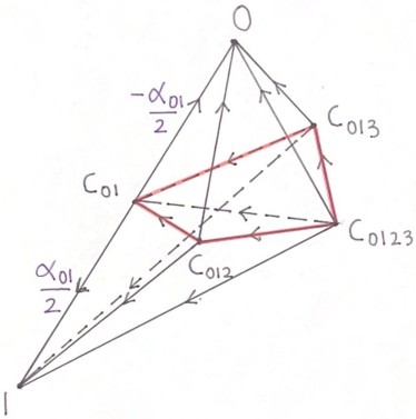
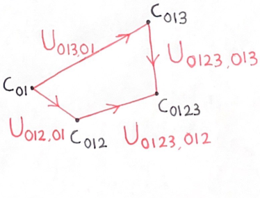
(A)		(B)

Figure 3. (A) Support volume of edge $[01]$ in a tetrahedron $[0123]$ (not shown). The CH-bundle curvature in the tetrahedron associated with this edge is the difference in transport along $c_{01}\to c_{012}\to c_{0123}$ and the transport along $c_{01}\to c_{013}\to c_{0123}$. This is recovered in our framework by subdividing the tetrahedron and computing $d_{\nabla}^{2}$ of a subdivided 1-form extended to some values following Remark 11.5 on subdivision edges that were not part of an original edge. (B) CH-bundle transports from the edge to the center of tetrahedron shown on the boundary of the dual of the edge.

Let $X$ be a simplicial complex of a tetrahedron $[0123]$. The elementary duals of, say vertex 0, are as follows. There is $(0-0)!=1$ elementary dual vertex of 0 in itself and it is $c_{0}=0$. There is $(1-0)!=1$ elementary dual edge of 0 in edge $[01]$ and it is $[c_{01},0]$. The elementary dual of 0 in edge $[02]$ is $[c_{02},0]$ etc. In a triangle, such as $[012]$, there are $(2-0)!=2$ elementary dual triangles of 0: $[c_{012},c_{01},0]$ and $[c_{012},c_{02},0]$. Similarly there are two such elementary dual triangles of 0 in each triangle containing 0. There are $(3-0)!=6$ elementary dual tetrahedra of 0 in $[0123]$. These are $[c_{0123}\,c_{012}\,c_{01}\,0]$, $[c_{0123}\,c_{012}\,c_{02}\,0]$, $[c_{0123}\,c_{013}\,c_{01}\,0]$, $[c_{0123}\,c_{013}\,c_{03}\,0]$, $[c_{0123}\,c_{023}\,c_{02}\,0]$ and $[c_{0123}\,c_{023}\,c_{03}\,0]$. There are $(3-1)!=2$ elementary dual triangles of $[01]$ in $[0123]$ and these are $[c_{0123}\,c_{012}\,c_{01}]$ and $[c_{0123}\,c_{013}\,c_{01}]$. The support volume $V_{01\prec 0123}$ of the edge $[01]$ in the tetrahedron consists of the four tetrahedra $[c_{0123}\,c_{012}\,c_{01}\,0]$, $[c_{0123}\,c_{013}\,c_{01}\,0]$, $[c_{0123}\,c_{012}\,c_{01}\,1]$ and $[c_{0123}\,c_{013}\,c_{01}\,1]$. See Figure 3 for an illustration of this support volume.

10.1. Vertex ordering and orientation in subdivision complex

For any $0\leq k\leq l\leq n$, the vertices of every elementary dual simplex of $\sigma^{k}$ in $\sigma^{l}$ will be defined to be totally ordered by a canonical total order given by $\hat{\sigma}^{l}<\hat{\sigma}^{l-1}<\ldots<\hat{\sigma}^{k}$. That is, the vertices are ordered in decreasing dimension of the simplex of which they are centers. With such a total ordering per simplex, the vertices of $\operatorname{sd}X$ acquire a partial order. For each $\sigma$ in $X$ the vertices of $\operatorname{sd}\sigma$ acquire the partial ordering as $\hat{\tau}^{j}<\hat{\tau}^{i}$ if $\tau^{i}\prec\tau^{j}$, $i<j$ for all simplices $\tau^{i}$ and $\tau^{j}$ in $\sigma$.

Example 10.2.

For a tetrahedron $\sigma=[0123]$, its subdivision $\operatorname{sd}\sigma$ consists of the vertex set $\{c_{0}=0,c_{1}=1,c_{2}=2,c_{3}=3,c_{01},c_{02},c_{03},c_{12},c_{13},c_{23},c_{012},c_{013},c_{023},c_{123},c_{0123}\}$ which become ordered as $0,1,2,3>c_{01},c_{02},c_{03},c_{12},c_{13},c_{23}>c_{012},c_{013},c_{023},c_{123}>c_{0123}$. Each of the 24 elementary dual tetrahedra in $\operatorname{sd}\sigma$ has a canonical total ordering on its vertices using the descending dimension ordering described above. For example, the vertices of the elementary dual tetrahedron $[c_{0123}\,c_{012}\,c_{01}\,0]$ are ordered in the order listed. Similarly, the vertices of any elementary dual simplex at any dimension $\leq 3$ are now totally ordered. For example, the vertices of $[c_{012}\,c_{01}\,0]$ are ordered as listed.

Given a primal simplex $\sigma^{k}$ the dual cell $\star\sigma^{k}$ and the support volume $V_{\sigma^{k}}$ inherit an orientation from the primal complex $X$. If the top dimensional simplices of $X$ are consistently oriented (as should be the case for an oriented manifold simplicial complex) the orientation of the entire cell $\star\sigma^{k}$ can be determined by first determining orientation of a single elementary dual simplex in $\star\sigma^{k}\cap\sigma^{n}$ for some $\sigma^{n}\succ\sigma^{k}$. Similarly for the support volume. See [22, Remark 2.5.1] for a procedure for assigning an orientation to the elementary dual simplices and hence to the dual cells in $\star X$ based on the orientations in $X$. This procedure is based on two ideas. The first idea is that the orientation of a $k$-dimensional elementary dual simplex $\tau$ in a subdivision of a $k$-dimensional primal simplex $\sigma$ can be compared to that of $\sigma$ since both $\tau$ and $\sigma$ are subsets of the $k$-dimensional affine space defined by either. The second idea is that given $\sigma^{k}\prec\sigma^{n}$, the simplices in the subdivision of $\sigma^{k}$ and those in the dual $\star\sigma^{k}\cap\sigma^{n}$ can be combined to form a top dimensional simplex whose orientation can be compared with that of $\sigma^{n}$. The next example illustrates how to orient a support volume once one elementary dual simplex orientation is fixed. This example uses a combinatorial procedure that supplements the discussion in [22].

Example 10.3.

As described in Example 10.1 the support volume of edge $[01]$ in tetrahedron $[0123]$ consists of the four elementary dual tetrahedra $[c_{0123}\,c_{012}\,c_{01}\,0]$, $[c_{0123}\,c_{013}\,c_{01}\,0]$, $[c_{0123}\,c_{012}\,c_{01}\,1]$ and $[c_{0123}\,c_{013}\,c_{01}\,1]$. In this example we will orient these starting with an orientation of $\tau=[c_{0123}\,c_{012}\,c_{01}\,0]$. Suppose the primal tetrahedron has the orientation of $[0123]$. Then following the ideas of [22, Section 2.5] the correct orientation of $\tau$ is as written above. To now orient $[c_{0123}\,c_{013}\,c_{01}\,0]$ we compare the orientations induced on the shared triangle $[c_{0123}\,c_{01}\,0]$. This is obtained by deleting vertex $c_{012}$ from $\tau$ and $c_{013}$ from $[c_{0123}\,c_{013}\,c_{01}\,0]$. This results in the same induced orientation for the shared triangle which should not be the case if the $n$-dimensional support volume object is to be consistently oriented. Thus the correct orientation is $-[c_{0123}\,c_{013}\,c_{01}\,0]$. This process can be continued until the remaining two tetrahedra of the support volume are oriented correctly. The correctly oriented tetrahedra are then $[c_{0123}\,c_{012}\,c_{01}\,0]$, $-[c_{0123}\,c_{013}\,c_{01}\,0]$, $-[c_{0123}\,c_{012}\,c_{01}\,1]$ and $[c_{0123}\,c_{013}\,c_{01}\,1]$ which together yield a consistently oriented support volume of $[01]$ in $[0123]$.

11. Relationship with Christiansen-Hu discrete vector bundles

Much of the work in this section was initially inspired by the elegant formalism of Christiansen and Hu [13]. We were pleased to discover that their definition of discrete covariant derivative and discrete curvature can be realized within our setup for a particular class of simplicial complex and a subspace of our $k$-cochains. This also suggested to us how curvature of a PL surface could be associated with the dual cell of a vertex, as is common in discrete differential geometry. See [28, 6] and references therein. More generally, we will be able to associate curvature of any simplex $\sigma^{k}$ with respect to a simplex $\sigma^{k+2}$ containing it.

While we fix a fiber per simplex by selecting an origin vertex per simplex Christiansen and Hu use an unspecified point in each simplex for placing the fibers. We will refer to Christiansen-Hu discrete vector bundles with connection as CH-bundles. While CH-bundles are defined for CW complexes, we will restrict to simplicial complexes. In a CH-bundle $E^{\textrm{CH}}$ over a simplicial complex $X$ the $k$-cochains will be referred to as $\alpha^{\textrm{CH}}\in C^{k}(X;E^{\textrm{CH}})$ and the discrete exterior covariant derivative as $d_{\nabla}^{\,\textrm{CH}}$. (This is denoted by $\delta_{t}$ in [13, Section 1.2].)

In this section we show that given $(E^{\textrm{CH}},\nabla^{\,\textrm{CH}})$ over $X$ there exists $(E,\nabla)$, a discrete vector bundle with connection (in our framework) over a subdivision $\operatorname{sd}X$ of $X$, in which all the objects and operators of CH-bundles can be reproduced. This is the content of Proposition 11.1. In §11.5 we discuss wedge product in the context of CH-bundles. In our framework a cup product is used as wedge product in Definition 6.1. However a naive duplication of this definition for the CH-bundles does not work. The use of a cup product leads to a curvature obstruction for Leibniz rule in the CH-bundles case. This is the content of Example 11.14. We then show a simple extension of CH-bundles which permits a new definition of a wedge product by assembling it from a subdivision. Under an appropriate hypothesis on subdivision this product then satisfies the Leibniz rule without any curvature obstruction. This is the content of Proposition 11.18.

Proposition 11.1 (Reproducing CH-bundles).

Given a CH-bundle $(E^{\textrm{CH}},\nabla^{\,\textrm{CH}})$ over a simplicial complex $X$, a CH-bundle cochain $\alpha^{\textrm{CH}}\in C^{k}(X;E^{\textrm{CH}})$ and a CH-bundle curvature homomorphism $F^{\textrm{CH}}$, there exists $(E,\nabla)$, a discrete vector bundle with connection over a subdivision $\operatorname{sd}X$ of $X$, and a cochain $\alpha\in C^{k}(\operatorname{sd}X;E)$ such that

1. $\langle d_{\nabla}^{\,\textrm{CH}}\alpha^{\textrm{CH}},\sigma^{k+1}\rangle_{c(\sigma^{k+1})}=\sum_{s\in\operatorname{sd}\sigma}\langle d_{\nabla}\alpha,s\rangle_{c(\sigma^{k+1})}$, where $s\in\operatorname{sd}X$ are of the same dimension and orientation as $\sigma^{k+1}\in X$, and

2. $\langle d^{2}_{\nabla}\alpha,V_{\sigma^{k}\prec\sigma^{k+2}}\rangle_{c(\sigma^{k+2})}=\langle F^{\textrm{CH}},\sigma^{k}\prec\sigma^{k+2}\rangle\langle\alpha,\sigma^{k}\rangle_{c(\sigma^{k})}$.

In (i) the terms $\langle d_{\nabla}\alpha,s\rangle_{c(\sigma)}$ are all in the fiber at the center of $\sigma$. This is because for all the $k$-simplices $s\in\operatorname{sd}\sigma$ the origin vertex is the center of $\sigma$ according to Remark 11.6. In (ii) the term $V_{\sigma^{k}\prec\sigma^{k+2}}$ is the support volume in $X$ of the codimension-2 face $\sigma^{k}$ of $\sigma^{k+2}\in X$ and $\langle F^{\textrm{CH}},\sigma^{k}\prec\sigma^{k+2}\rangle$ means evaluation of the CH-bundle curvature associated with $\sigma^{k}$ in $\sigma^{k+2}$. This is a homomorphism from the fiber at $c(\sigma^{k})$ to that at $c(\sigma^{k+2})$.

Before giving the proof we give some constructions needed to prove these propositions and some examples to illustrate the main ideas of the proof that follows.

11.1. Parallel transports on a subdivision

Transports in the CH-bundle $E^{\textrm{CH}}$ over simplicial complex $X$ are $U_{c(\sigma^{k+1})\,c(\sigma^{k})}$ from center $c(\sigma^{k})$ of a $k$-dimensional simplex $\sigma^{k}$ to $c(\sigma^{k+1})$ where $\sigma^{k}\prec\sigma^{k+1}$ and $0\leq k<n$ . In the corresponding bundle $E$ over $\operatorname{sd}X$ in our framework, the transports are $U_{c(\sigma^{l})c(\sigma^{k})}$, with $0\leq k<l\leq n$, and $\sigma^{k}\prec\sigma^{l}$. These are defined to be the transports of $E^{\textrm{CH}}$ if $l=k+1$. For $l\neq k+1$, in constructing $E$ these maps are set to be arbitrary isomorphisms between the fibers $E_{c(\sigma^{k})}$ and $E_{c(\sigma^{l})}$. The terms involving these maps cancel when used in reproducing CH-bundles in our framework and hence can be arbitrary. One possibility is to determine these parallel transport via the same discretization or other process that was used in determining the parallel transports needed in CH-bundles. Sometimes we will write the transport $U_{c(\sigma^{k+1})\,c(\sigma^{k})}$ as $U_{\sigma^{k+1}\sigma^{k}}$ or $U_{\sigma^{k+1},\sigma^{k}}$ for notational simplicity. Furthermore, as before we will drop the square brackets when referring to a specific simplex by its vertices in a transport map. For example $U_{012,02}$ instead of $U_{[012],[02]}$ which in turn stands for $U_{c(012),\,c(02)}$.

Example 11.2.

Let $X$ be the simplicial complex of a tetrahedron $[0123]$. Transports in $E^{\textrm{CH}}$ over $X$ are the following:

1. $U_{c(e)\,c(v)}$ where $e\in\{[01],[02],[03],[12],[13],[23]\}$ is an edge of $[0123]$ and $v$ is a vertex of that edge. For a vertex $v$ the center $c(v)=v$.

2. $U_{c(f)\,c(e)}$ where $f$ is any of the four triangles of $[0123]$ and $e$ is an edge of that triangle.

3. $U_{c(0123)\,c(f)}$ where $f$ is any triangle of $[0123]$.

These may be written in the simpler notation as $U_{e,v}$, $U_{f,e}$, $U_{0123,f}$, respectively. Transports in $E$ over $X$ are the ones above and in addition $U_{c(f),v}$, $U_{c(0123),v}$ and $U_{c(0123),c(e)}$ and these are all arbitrary isomorphisms between the appropriate fibers or are obtained by the same procedure that yielded the original CH-bundle transports.

11.2. Cochains on a subdivision

Corresponding to $k$-cochains in $E^{\textrm{CH}}$ over $X$ we define $k$-cochains in $E$ over a subdivision $\operatorname{sd}X$ by defining a map $\mathcal{S}_{k}:C^{k}(X;E^{\textrm{CH}})\to C^{k}(\operatorname{sd}X;E)$ as follows. The same notation and definition is used for scalar valued cochains, that is for $\mathcal{S}_{k}:C^{k}(X)\to C^{k}(\operatorname{sd}X)$.

Definition 11.3.

Let $\alpha^{\textrm{CH}}\in C^{k}(X;E^{\textrm{CH}})$ and $\sigma$ a $k$-simplex in $X$. Let $s_{i}\in\operatorname{sd}X$, $i\in\{1,\ldots,(k+1)!\}$ be the collection of $k$-simplices in the subdivision $\operatorname{sd}\sigma$ and let these be oriented the same as $\sigma$. Define $\alpha:=\mathcal{S}_{k}(\alpha^{\textrm{CH}})\in C^{k}(\operatorname{sd}X;E)$, the cochain subdivision of $\alpha^{\textrm{CH}}$ by defining its value on $s_{i}$ as $\langle\alpha,s_{i}\rangle:=a_{i}\langle\alpha^{\textrm{CH}},\sigma\rangle$ where $0<a_{i}<1$ are fractions such that $\sum_{i=1}^{(k+1)!}a_{i}=1$. See Remark 11.4 on how to choose these fractions. If $s\in\operatorname{sd}X$ is a $k$-simplex that is not in $\operatorname{sd}\sigma$ for any $k$-simplex $\sigma$ of $X$ then define $\langle\alpha,s\rangle$ following Remark 11.5. The same definition applies to cochain subdivision of scalar valued cochains $C^{k}(X)$.

Remark 11.4.

How the fractions $a_{i}$ of Definition 11.3 are chosen may depend on future applications and/or the type of centers used. For reproducing $d_{\nabla}^{\,\textrm{CH}}$ and the curvature $E^{\textrm{CH}}$ of CH-bundles any choice works as long as the fractions sum to 1 over the subdivisions of a simplex. For simplicity we use $a_{i}^{\sigma}=1/(k+1)!$ for all $s_{i}$ in given $\operatorname{sd}\sigma\subset\operatorname{sd}X$ in all examples in this paper. An alternative could be, for example, to partition according to the proportion of $k$-dimensional volumes $|s_{i}|/|\sigma|$. For a given $k$-form that is being discretized could discretize following Remark 3.3 not on $X$ but on the subdivision. Of course that is not relevant when a given cochain is being subdivided.

Remark 11.5.

The values of $\langle\alpha,s\rangle$ when $s$ is not obtained from a subdivision of a simplex in $X$ do not have any constraints as far as reproduction of $d_{\nabla}^{\,\textrm{CH}}$ and $E^{\textrm{CH}}$ using our framework is concerned. However for defining a wedge product for CH-bundles in §11.5 the values for such simplices should in some way depend on the data. For example, $\langle\alpha,s\rangle$ may be obtained from an interpolation and integration procedure as follows. Using the local trivialization described in Remark 3.3 the components of $\alpha^{\textrm{CH}}$ can be interpolated using, for example, Whitney forms [7, 16] to obtain a smooth vector bundle valued form in a top dimensional simplex containing $s$. This can then be discretized as in Remark 3.3 to obtain $\langle\alpha,s\rangle$. As in Remark 11.4 a given vector bundle valued $k$-form could also be discretized on the subdivision.

Remark 11.6.

Given a $\sigma^{k}\prec\sigma^{l}$ we will choose $\hat{\sigma}^{l}$ as the origin vertex for all the elementary duals of $\sigma^{k}$ in $\sigma^{l}$ and choose $\hat{\sigma}^{k}$ as the destination vertex. The partial ordering of vertices in $\operatorname{sd}X$ described in §10.1 is designed so that with the choice of the origin vertex made here, the subdivided parts of a cochain in $E^{\textrm{CH}}$ over $X$ are elements of the same vector space in $E$ over $\operatorname{sd}X$.

The following example illustrates the partitioning of cochain values as well as the point about the origin vertices. See also Figure 2.

Example 11.7.

Let $X$ be the simplicial complex of a triangle $[012]$, and consider cochains $\alpha^{\textrm{CH}}\in C^{0}(X;E^{\textrm{CH}})$, $\beta^{\textrm{CH}}\in C^{1}(X;E^{\textrm{CH}})$ and $\gamma^{\textrm{CH}}\in C^{2}(X;E^{\textrm{CH}})$. If $\alpha^{\textrm{CH}}$ takes the values $\alpha_{i}$ on vertex $i=0,1,2$, the corresponding $\alpha\in C^{0}(\operatorname{sd}X;E)$ in our framework is defined to have the same values at vertices 0,1 and 2 and values at the other vertices of $\operatorname{sd}X$ following Remark 11.5.

Let $\beta_{01}=\langle\beta^{\textrm{CH}},[01]\rangle$ be the value of the 1-cochain on edge $[01]$ which is an element of $E_{c(01)}$ in the CH-bundle. The associated cochain $\beta\in C^{1}(\operatorname{sd}X;E)$ takes on values on the two edges $[c_{01}0]$ and $[c_{01}1]$ of $\operatorname{sd}X$ obtained by subdividing $[01]$ in $X$. These values are $\langle\beta,[c_{01}0]\rangle=-\beta_{01}/2\in E_{c(01)}$ and $\langle\beta,[c_{01}1]\rangle=\beta_{01}/2\in E_{c(01)}$. Then if the value on the original edge $[01]$ is needed, it is $\langle\beta,[01]\rangle=-\langle\beta,[c_{01}0]\rangle+\langle\beta,[c_{01}1]\rangle=\beta_{01}$. The addition is allowed since both parts of the original $\beta_{01}$ are elements of the same vector space $E_{c(01)}$ in the subdivision. The minus sign used with $\langle\beta,[c_{01}0]\rangle$ has to do with orientation rules described in §10.1.

For the edges $e$ of $\operatorname{sd}X$ that do not result from the subdivision of an edge of $X$ the values $\langle\beta,e\rangle$ are obtained as in Remark 11.5. The edges between the center of the triangle and centers of edges and vertices are all examples of such edges as shown in Figure 2 (A).

Finally consider a 2-cochain $\gamma^{\textrm{CH}}\in C^{2}(X;E^{\textrm{CH}})$ with the associated cochain $\gamma\in C^{2}(\operatorname{sd}X;E)$. Assuming equal partitioning, the value $\langle\gamma^{\textrm{CH}},[012]\rangle$ in $E_{c[012]}$ is partitioned into $(2+1)!$ parts as

(38) $$-\langle\gamma,[c_{012}c_{01}0]\rangle=\langle\gamma,[c_{012}c_{02}0]\rangle=\langle\gamma,[c_{012}c_{01}1]\rangle=-\langle\gamma,[c_{012}c_{12}1]\rangle=\langle\gamma,[c_{012}c_{12}2]\rangle\\ =-\langle\gamma,[c_{012}c_{02}2]\rangle=\frac{1}{6}\langle\gamma^{\textrm{CH}},[012]\rangle\,.$$

All these triangles in the subdivision of $[012]$ share the vertex $c_{012}$ at the center of the original triangle $[012]$ and thus the values of $\gamma$ on the smaller triangles all reside at the same vertex $c_{012}$ in the bundle $E$ over $\operatorname{sd}X$. This is the origin vertex for all these small triangles since $c_{012}$ is the smallest in the total ordering of vertices of each of the small triangles as per §10.1.

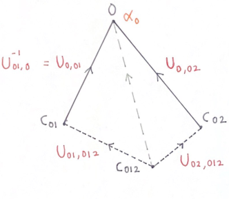
(A)		(B)

Figure 2. (A) Cochains in our framework obtained from CH-bundle cochains. For example, the CH bundle 1-cochain $\beta$ with value $\beta_{01}$ on $[01]$ results in $\beta_{01}/2$ magnitude values on the subdivision. The signs depend on the orientation of the smaller edges. Magnitudes need not be equal, but must add up to $\beta_{01}$. Values on dashed edges are set as per Remark 11.5 and are not shown. Due to the ordering of centers, all the values in a subdivided simplex are in the fiber at the center and add up to the value on the undivided simplex, reproducing the CH-bundle setup when added. For example, all the $\gamma$ values for the small triangles are in the fiber at the center $c_{012}$ of the triangles. See Example 11.7. (B) The support volume of vertex 0 used in the curvature computation in Example 11.10.

11.3. Reproducing CH-bundle exterior covariant derivative

Let $\alpha^{\textrm{CH}}\in C^{k}(X;E^{\textrm{CH}})$ and $\alpha\in C^{k}(\operatorname{sd}X;E)$ the corresponding cochain in our framework as in §11.2. As stated in Proposition 11.1

$$\langle d_{\nabla}^{\,\textrm{CH}}\alpha^{\textrm{CH}},\sigma^{k+1}\rangle=\sum_{s\in\operatorname{sd}\sigma^{k+1}}\langle d_{\nabla}\alpha,s\rangle\,,$$

where $s\in\operatorname{sd}X$ is oriented the same as $\sigma^{k+1}\in X$. The next example illustrates this with for 0-cochain.

Example 11.8.

Let $X$ and $\alpha^{\textrm{CH}}$ be as in Example 11.7. Then $\langle d_{\nabla}\alpha,[c_{01}0]\rangle=U_{01,0}\alpha_{0}-\alpha_{c_{01}}$ and $\langle d_{\nabla}\alpha,[c_{01}1]\rangle=U_{01,1}\alpha_{1}-\alpha_{c_{01}}$. To compare with $\langle d_{\nabla}^{\,\textrm{CH}}\alpha^{\textrm{CH}},[01]\rangle$ we must add the two above values with an appropriate sign since the chain $[01]=[0\,c_{01}]+[c_{01}\,1]=-[c_{01}\,0]+[c_{01}\,1]$. Thus

$$\langle d_{\nabla}\alpha,[01]\rangle =-\langle d_{\nabla}\alpha,[c_{01}\,0]\rangle+\langle d_{\nabla}\alpha,[c_{01}\,1]\rangle$$

$$=-U_{01,0}\alpha_{0}+\alpha_{c_{01}}+U_{01,1}\alpha_{1}-\alpha_{c_{01}}=U_{01,1}\alpha_{1}-U_{01,0}\alpha_{0}$$

which is the same as $\langle d_{\nabla}^{\,\textrm{CH}}\alpha^{\textrm{CH}},[01]\rangle$.

Remark 11.9.

Note that the values of $\alpha$ on vertices of $\operatorname{sd}X$ that are not vertices of $X$ cancel. This is an example of the general phenomena in reproducing $d_{\nabla}^{\,\textrm{CH}}$ using $d_{\nabla}$ in that the values of the $k$-cochain on $k$-simplices of $\operatorname{sd}X$ that do not arise from subdividing a $k$-simplex of $X$ cancel. See proof of Proposition 11.1(i).

11.4. Reproducing CH-bundle curvature

Given a $k$-dimensional simplex $\sigma$, $2\leq k\leq n$ and a codimension 2 face $\tau$ of $\sigma$, the CH-bundles curvature defined in [13] is a homomorphism defined on the pair $\tau\prec\sigma$ and we will rephrase this in terms of primal-dual complexes. For CH-bundles the curvature is associated with the 2-dimensional cell that would be the dual of $\tau$ in $\sigma$. We will rephrase this curvature associated with $\tau$ in $\sigma$ by defining it on $\star\tau\cap\sigma$ as follows. Let $\rho_{+}$ and $\rho_{-}$ be the two codimension 1 faces of $\sigma$ that contain $\tau$. Then the CH-bundle curvature $F^{\textrm{CH}}$ is $U_{\sigma\,\rho_{+}}\,U_{\rho_{+}\,\tau}-U_{\sigma\,\rho_{-}}U_{\rho_{-}\,\tau}$. The plus-minus labelling of $\rho_{\pm}$ depends on the orientations. It is shown in [13] that $F^{\textrm{CH}}=d_{\nabla}^{\,\textrm{CH}}\circ d_{\nabla}^{\,\textrm{CH}}$. We show here that the curvature in a CH-bundle $E^{\textrm{CH}}$ over $X$ can be reproduced using $d_{\nabla}$ on $E$ over $\operatorname{sd}X$ in our framework. This formulated in Proposition 11.1 above as

$$\langle d^{2}_{\nabla}\alpha,V_{\sigma^{k}\prec\sigma^{k+2}}\rangle=\langle F^{\textrm{CH}},\sigma^{k}\prec\sigma^{k+2}\rangle\langle\alpha,\sigma^{k}\rangle\,,$$

where $\langle F^{\textrm{CH}},\sigma^{k}\prec\sigma^{k+2}\rangle$ is the CH-bundle curvature $F^{\textrm{CH}}$ on the codimension-2 face $\sigma^{k}$ of a dimension $k+2$ simplex $\sigma^{k+2}$.

Since $d_{\nabla}^{2}$ raises the degree of a cochain by 2, for $\alpha\in C^{k}(\operatorname{sd}X,E)$ the cochain $d_{\nabla}^{2}\alpha$ has to be evaluated on a cell of dimension $k+2$. If $\tau\prec\sigma$ is the pair of simplices with $\tau$ a codimension 2 face of $\sigma$ then we will recover the curvature associated with this pair by evaluating $d_{\nabla}^{2}\alpha$ on the support volume $V_{\tau\prec\sigma}$. The next example shows this computation for the simplest case, in which $k=0$.

Example 11.10.

Let $X$ be the simplicial complex of a triangle $[012]$. Then the curvature associated with vertex 0 in the CH-bundles theory is the homomorphism valued object $F=U_{012,02}\,U_{02,0}-U_{012,01}\,U_{01,0}$. This can be reproduced on $\operatorname{sd}X$ in our framework as follows. See also the accompanying Figure 2(B). Let $\alpha^{\textrm{CH}}$ be the 0-cochain of Example 11.8. We will compute $\langle d_{\nabla}^{2}\alpha,V_{0\prec 012}\rangle$ in our framework and see that this is the same as $F\alpha$ thus reproducing the curvature of CH-bundles using our framework. The cell $V_{0\prec 012}$ on which the evaluation is being done is of dimension 2 and is the same as $\star 0$, the dual of the vertex 0 in the triangle in this case. We start with

(39) $$\langle d_{\nabla}^{2}\alpha,V_{0\prec 012}\rangle=\langle d_{\nabla}^{2}\alpha,[0\,c_{01}\,c_{012}]\rangle+\langle d_{\nabla}^{2}\alpha,[c_{012}\,c_{02}\,0]\rangle\,,$$

where the two terms on the RHS are evaluated at $c_{012}$ since that comes first in the partial order of §10.1. The two triangles in $\operatorname{sd}X$ that constitute $\star 0$ are oriented counterclockwise to match the orientation of $[012]$. The first term on the RHS is

$$\langle d_{\nabla}^{2}\alpha,[0\,c_{01}\,c_{012}]\rangle=\langle d_{\nabla}\alpha,[c_{01}\,c_{012}]\rangle-\langle d_{\nabla}\alpha,[0\,c_{012}]\rangle+U_{012,01}\langle d_{\nabla}\alpha,[0\,c_{01}]\rangle\,.$$

The first two RHS terms above are in the vector space at $c_{012}$ so do not need to be transported. Thus

(40) $$\langle d_{\nabla}^{2}\alpha,[0\,c_{01}\,c_{012}]\rangle =\alpha_{c_{012}}-U_{012,01}\alpha_{c_{01}}-(\alpha_{c_{012}}-U_{012,0}\alpha_{0})+U_{012,01}(\alpha_{c_{01}}-U_{01,0}\alpha_{0})$$

$$=U_{012,0}\alpha_{0}-U_{012,01}\,U_{01,0}\,\alpha_{0}\,.$$

The second term in the RHS of (39) is

$$\langle d_{\nabla}^{2}\alpha,[c_{012}\,c_{02}\,0]\rangle=U_{012,02}\langle d_{\nabla}\alpha,[c_{02}\,0]\rangle-\langle d_{\nabla}\alpha,[c_{012}\,0]\rangle+\langle d_{\nabla}\alpha,[c_{012}\,c_{02}]\rangle\,.$$

As in the expansion of the first term of (39), the terms on edges with one vertex at $c_{012}$ do not need to be transported. Thus

(41) $$\langle d_{\nabla}^{2}\alpha,[c_{012}\,c_{02}\,0]\rangle =U_{012,02}(U_{02,0}\alpha_{0}-\alpha_{c_{02}})-(U_{012,0}\alpha_{0}-\alpha_{c_{012}})+(U_{012,02}\alpha_{c_{02}}-\alpha_{c_{012}})$$

$$=U_{012,02}\,U_{02,0}\,\alpha_{0}-U_{012,0}\alpha_{0}\,.$$

Putting (40) and (41) together in (39)

$$\langle d_{\nabla}^{2}\alpha,V_{0\prec 012}\rangle=(U_{012,02}\,U_{02,0}-U_{012,01}\,U_{01,0})\alpha_{0}\,,$$

which is precisely $F\alpha_{0}$ as in CH-bundles.

Remark 11.11.

As in Remark 11.9 the above example illustrates that the values of $\alpha$ on vertices of $\operatorname{sd}X$ that are not vertices of $X$ cancel. As before, this is also a general phenomena in all dimensions. See Proof of Proposition 11.1.

To illustrate the reproduction of the CH-bundle curvature and the cancelation phenomena remarked above in higher dimensions the next example shows the computation of the curvature associated with an edge in a tetrahedron, i.e., when $k=1$.

Example 11.12.

Let $X$ be the simplicial complex of a tetrahedron $[0123]$ and $\alpha^{\textrm{CH}}\in C^{1}(X;E^{\textrm{CH}})$ and $\mathcal{S}_{1}(\alpha^{\textrm{CH}})=\alpha\in C^{1}(\operatorname{sd}X;E)$ the corresponding cochain in our framework. Following the procedure in §11.2 the 1-cochain $\alpha$ in the vector bundle over the subdivision $\operatorname{sd}X$ is obtained by setting its value on edges of the subdivision that are not part of an original edge of $X$ as in Remark 11.5. On the edges in $\operatorname{sd}X$ that are the result of subdivision of edges of $X$, the value of $\alpha$ is set by dividing the value of $\alpha^{\textrm{CH}}$ on the parent edge between the smaller edges of $\operatorname{sd}X$ as in Remark 11.4. Thus for example, if $\alpha^{\textrm{CH}}_{01}=\langle\alpha^{\textrm{CH}},[01]\rangle$ in the CH-bundle, in $(\operatorname{sd}X;E)$ we can take the magnitude of the evaluation of $\alpha$ on the smaller edges $[c_{01}\,0]$ and $[c_{01}\,1]$ to be such that they add up to the magnitude of $\alpha^{\textrm{CH}}$ and then $\langle\alpha^{\textrm{CH}},[01]\rangle=\langle\alpha,[01]\rangle=-\langle\alpha,[c_{01}\,0]\rangle+\langle\alpha,[c_{01}\,1]\rangle$.

The CH-bundle curvature associated with edge $[01]$ in $[0123]$ is $U_{0123,013}\,U_{013,01}-U_{0123,012}\,U_{012,01}$ and is associated with the dual of edge $[01]$ in $[0123]$. We will reproduce this by computing the 3-cochain $d_{\nabla}^{2}\alpha$ on the support volume $V_{01\prec 0123}$ of the edge in the tetrahedron. A consistent orientation of the four elementary dual tetrahedra in $V_{01\prec 0123}$ that agrees with the orientation of the containing tetrahedron $[0123]$ was given in Example 10.3. Two of the subdivision tetrahedra in $V_{01\prec 0123}$ form the underlying space of $\star 0\cap V_{01\prec 0123}$ and the other two that of $\star 1\cap V_{01\prec 0123}$. The two tetrahedra in $\star 0\cap V_{01\prec 0123}$ are $[c_{0123}\,c_{012}\,c_{01}\,0]$ and $[c_{0123}\,c_{013}\,c_{01}\,0]$ corresponding to the two triangles $[012]$ and $[013]$ containing the edge $[01]$. Similarly, the two tetrahedra in $\star 1\cap V_{01\prec 0123}$ are $[c_{0123}\,c_{012}\,c_{01}\,1]$ and $[c_{0123}\,c_{013}\,c_{01}\,1]$.

The CH-bundle curvature associated with the edge $[01]$ is reproduced by

(42) $$\langle d_{\nabla}^{2}\alpha,V_{01\prec 0123}\rangle=\langle d_{\nabla}^{2}\alpha,[c_{0123}\,c_{012}\,c_{01}\,0]\rangle-\langle d_{\nabla}^{2}\alpha,[c_{0123}\,c_{013}\,c_{01}\,0]\rangle-\\ \langle d_{\nabla}^{2}\alpha,[c_{0123}\,c_{012}\,c_{01}\,1]\rangle+\langle d_{\nabla}^{2}\alpha,[c_{0123}\,c_{013}\,c_{01}\,1]\rangle\,,$$

where the signs for the terms in the RHS follow the orientation in Example 10.3. All terms on both sides are in the fiber at $c_{0123}$. The first term on the RHS is

(43) $$U_{0123,012}\langle d_{\nabla}\alpha,[c_{012}\,c_{01}\,0]\rangle-\langle d_{\nabla}\alpha,[c_{0123}\,c_{01}\,0]\rangle+\langle d_{\nabla}\alpha,[c_{0123}\,c_{012}\,0]\rangle-\langle d_{\nabla}\alpha,[c_{0123}\,c_{012}\,c_{01}]\rangle\,,$$

in which the last three terms do not need to be transported since they are in the fiber at $c_{0123}$. The other three terms in (42) are similar with the appropriate substitutions for the digits. The terms in (43) evaluate to the following:

$$U_{0123,012}\langle d_{\nabla}\alpha,[c_{012}\,c_{01}0]\rangle =U_{0123,012}\big{(}U_{012,01}\langle\alpha,[c_{01}\,0]\rangle-\langle\alpha,[c_{012}\,0]\rangle+\langle\alpha,[c_{012}\,c_{01}]\rangle\big{)}$$

$$-\langle d_{\nabla}\alpha,[c_{0123}\,c_{01}\,0]\rangle =-\big{(}U_{0123,01}\langle\alpha,[c_{01}\,0]\rangle-\langle\alpha,[c_{0123}\,0]\rangle+\langle\alpha,[c_{0123}\,c_{01}]\rangle\big{)}$$

$$\langle d_{\nabla}\alpha,[c_{0123}\,c_{012}\,0]\rangle =U_{0123,012}\langle\alpha,[c_{012}\,0]\rangle-\langle\alpha,[c_{0123}\,0]\rangle+\langle\alpha,[c_{0123}\,c_{012}]\rangle$$

$$-\langle d_{\nabla}\alpha,[c_{0123}\,c_{012}\,c_{01}]\rangle =-\big{(}U_{0123,012}\langle\alpha,[c_{012}\,c_{01}]\rangle-\langle\alpha,[c_{0123}\,c_{01}]\rangle+\langle\alpha,[c_{0123}\,c_{012}]\rangle\big{)}$$

Adding these yields

$$\langle d_{\nabla}^{2}\alpha,[c_{0123}\,c_{012}\,c_{01}\,0]\rangle=U_{0123,012}U_{012,01}\langle\alpha,[c_{01}0]\rangle-U_{0123,01}\langle\alpha,[c_{01}0]\rangle\,,$$

and the other three terms on the RHS in (42) yield similar expressions with appropriate digit substitutions. Substituting these in the RHS of (42) and collecting terms yields

$$\langle d_{\nabla}^{2}\alpha,V_{01\prec 0123}\rangle=\bigl{(}U_{0123,012}U_{012,01}-U_{0123,013}U_{013,01}\bigr{)}\langle\alpha,[c_{01}0]\rangle+\\ \bigl{(}U_{0123,013}U_{013,01}-U_{0123,012}U_{012,01}\bigr{)}\langle\alpha,[c_{01}1]\rangle\,.$$

Finally using the fact that $\langle\alpha,[c_{01}0]\rangle=-\alpha_{01}/2$ and $\langle\alpha,[c_{01}1]\rangle=\alpha_{01}/2$ we have

(44) $$\langle d_{\nabla}^{2}\alpha,V_{01\prec 0123}\rangle=\bigl{(}U_{0123,013}U_{013,01}-U_{0123,012}U_{012,01}\bigr{)}\alpha_{01}\,.$$

As indicated in Remark 11.4, the fact that $\langle\alpha,[01]\rangle$ has been partitioned into two equal parts in the above computation is not important. Any two positive fractions that add up to 1 would have sufficed.

The transport in (44) is precisely the CH-bundle curvature associated with the edge $[01]$ in tetrahedron $[0123]$. As in the CH-bundle case, the curvature is the difference in transport from the center of edge $[01]$ to center of $[0123]$. The transport $U_{0123,013}U_{013,01}$ is along two edges of the boundary of the combinatorial quadrilateral that is the dual of the edge $[01]$. The transport $U_{0123,013}U_{013,01}$ is along the other two edges of the quadrilateral boundary.

The statement of Proposition 11.1(ii) involves simplices $\sigma^{k}$ and $\sigma^{k+2}$. This is because the discrete curvature homomorphism makes sense for any codimension-2 simplex. In the Examples 11.10 and 11.12 the higher dimension is $n$, the top dimension. To clarify the more general geometric picture we next consider the case of $n=7$ and $k=2$.

Example 11.13.

Let $X$ be the simplicial complex of the simplex $[0\,...\,7]$ and $[012]$ a triangle in $X$. Then the value of a 2-cochain $\alpha^{\textrm{CH}}\in C^{2}(X;E^{\textrm{CH}})$ in the CH-bundle is subdivided according to Remark 11.4. This results in values of the corresponding cochain $\mathcal{S}_{2}(\alpha^{\textrm{CH}})=\alpha\in C^{2}(\operatorname{sd}X;E)$ in our framework on the smaller subdivision triangles $s\in[012]$. For the evaluation $\langle d^{2}_{\nabla}\alpha,V_{\sigma^{k}\prec\sigma^{k+2}}\rangle_{c(\sigma^{k+2})}$ in Proposition 11.1 we have to choose a specific dimension 4 simplex containing $[012]$. Suppose this is $[01234]$. Then the support volume $V_{012\prec 01234}$ consists of 12 dimension 4 elementary dual simplices. These come in 6 pairs of 2 simplices, with each of the 6 corresponding to a subdivision triangle of $[012]$. For example, one such subdivision triangle is $[c_{012}\,c_{01}\,0]$ (see Figure 2). The pair of 4 dimensional simplices associated with this subdivision triangle are $[c_{01234}\,c_{0123}\,c_{012}\,c_{01}\,0]$ and $[c_{01234}\,c_{0124}\,c_{012}\,c_{01}\,0]$. The triangle $[012]$ is the face of exactly two tetrahedra in $[01234]$. These are $[0123]$ and $[0124]$ and the centers of these two are used in the pair of 4-dimensional simplices given above.

In general, for a fixed $k$-simplex $\sigma^{k}$ that is a face of a fixed $(k+2)$-dimensional simplex $\sigma^{k+2}$ the $(k+2)$-dimensional simplices that make up the support volume $V_{\sigma^{k}\prec\sigma^{k+2}}$ are all the simplices of the form

(45) $$[c(\sigma^{k+2})\,c(\sigma^{k+1})\,c(\sigma^{k})\,c(\sigma^{k-1})\,\ldots c(\sigma^{1})\,c(\sigma^{0})]\,.$$

Here only $\sigma^{k+2}$ and $\sigma^{k}$ are fixed and we consider all possibilities for the simplices of the other dimensions such that $\sigma^{0}\prec\sigma^{1}\prec\ldots\prec\sigma^{k+2}$. As we will see in the proof of Proposition 11.1(ii), in the computation of $\langle d^{2}_{\nabla}\alpha,V_{\sigma^{k}\prec\sigma^{k+2}}\rangle_{c(\sigma^{k+2})}$ the transports will involve the first 3 centers in (45) and the subdivision simplices will involve the last $k+1$ centers in (45).

We now give the proof of Proposition 11.1. In this proof we will use the following conventions and notation. Whenever a symbol for a simplex makes it first appearance its dimension will be in the superscript unless it is stated in text. Any oriented $k$-simplex $s$ induces an orientation on each of its $(k-1)$-dimensional face $t$ which can be symbolically deduced by deleting a vertex in the vertex ordering of $s$. If the orientation induced agrees with the given orientation of $t$ then the term $o(t,s)$ that appears in the proof below is $+1$ and otherwise it is $-1$. The origin vertex of a simplex $t$ will be denoted $v(t)$.

Proof of Proposition 11.1(i).

Using the definition of $d_{\nabla}$ the RHS of (i) is

$$\sum_{s\in\operatorname{sd}\sigma}\langle d_{\nabla}\alpha,s\rangle_{c(\sigma)}=\sum_{s\in\operatorname{sd}\sigma}\;\sum_{t^{k}\prec s}o(t,s)U_{c(\sigma),v(t)}\langle\alpha,t\rangle_{v(t)}\,.$$

If $t\cap\partial\sigma=\emptyset$ then the origin vertex $v(t)$ of $t$ is the center $c(\sigma)$ according to Remark 11.6. If $t\cap\partial\sigma\neq\emptyset$ then $t\in\tau^{k-1}\prec\sigma$ in $\partial\sigma$ and then the origin vertex of $t$ is $c(\tau)$ by Remark 11.6.

The RHS of the sum above can be split into two summations, one over $t$ s.t. $t\cap\partial\sigma=\emptyset$ and the other over the rest. The the RHS above becomes

(46) $$\sum_{s\in\operatorname{sd}\sigma}\bigg{(}\sum_{\begin{subarray}{c}t\prec s\\ r\cap\partial\sigma=\emptyset\end{subarray}}o(t,s)\langle\alpha,t\rangle_{c(\sigma)}\bigg{)}+\sum_{s\in\operatorname{sd}\sigma}\bigg{(}\sum_{\begin{subarray}{c}t\prec s\\ t\cap\partial\sigma\neq\emptyset\end{subarray}}o(t,s)U_{c(\sigma),v(t)}\langle\alpha,t\rangle_{v(t)}\bigg{)}\,.$$

The first summation term of (46) can be reordered and written in terms of the $(k-1)$-simplices $t$ as

$$\sum_{\begin{subarray}{c}t\in\operatorname{sd}\sigma\\ t\cap\partial\sigma=\emptyset\end{subarray}}o(t,s^{+})\langle\alpha,t\rangle_{c(\sigma)}+o(t,s^{-})\langle\alpha,t\rangle_{c(\sigma)}\,,$$

where $s^{+}$ and $s^{-}$ are the two $k$-dimensional simplices of $\operatorname{sd}\sigma$ with the shared face $t$. Since $o(t,s^{+})=-o(t,s^{-})$ the terms in this sum are all 0. The second summation term of (46) can be reordered so that the terms are collected according to the $k$-dimensional faces $\tau$ of $\sigma$ containing the $k$-dimensional simplices $t$ of $\operatorname{sd}\sigma$. For all $t$ in such a $\tau$ the orientations will all agree with $o(\tau,\sigma)$. For such a $t$ the origin vertex $v(t)=c(\tau)$ so the second summation of (46) becomes

$$\sum_{\tau\prec\sigma}\sum_{t\in\operatorname{sd}\tau}o(\tau,\sigma)U_{c(\sigma),c(\tau)}\langle\alpha,t\rangle_{c(\tau)} =\sum_{\tau\prec\sigma}o(\tau,\sigma)U_{c(\sigma),c(\tau)}\sum_{t\in\operatorname{sd}\tau}\langle\alpha,t\rangle_{c(\tau)}$$

$$=\sum_{\tau\prec\sigma}o(\tau,\sigma)U_{c(\sigma),c(\tau)}\langle\alpha^{\textrm{CH}},\tau\rangle_{c(\tau)}=\langle d_{\nabla}^{\,\textrm{CH}}\alpha^{\textrm{CH}},\sigma\rangle_{c(\sigma)}$$

∎

Proof of Proposition 11.1(ii).

With $\sigma^{k}\prec\sigma^{k+2}$ both fixed there are exactly two $(k+1)$-simplices, say $\sigma^{k+1}_{+}$ and $\sigma^{k+1}_{-}$ such that $\sigma^{k}\prec\sigma^{k+1}_{\pm}\prec\sigma^{k+2}$. Now consider one of the $(k+1)!$ subdivision $k$-simplices of $\sigma^{k}$. For each such subdivision simplex $s=[c(\sigma^{k})\,\ldots\,c(\sigma^{1})\,c(\sigma^{0})]$ there are two $(k+2)$-dimensional simplices in $V_{\sigma^{k}\prec\sigma^{k+2}}$ containing $s$ and these are $\tau_{\pm}=[c(\sigma^{k+2})\,c(\sigma_{\pm}^{k+1})\,c(\sigma^{k})\,\ldots\,c(\sigma^{1})\,c(\sigma^{0})]$. By Remark 11.6 the origin vertex of all the $(k+2)$-dimensional simplices in $V_{\sigma^{k}\prec\sigma^{k+2}}$ is $c(\sigma^{k+2})$ and the origin vertex of all the subdivision $k$-simplices of $\sigma^{k}$ is $c(\sigma^{k})$. By the proof of Proposition 8.7

$$\langle d_{\nabla}^{2}\alpha,\tau_{\pm}\rangle_{c(\sigma^{k+2})}=\big{(}U_{c(\sigma^{k+2}),\,c(\sigma^{k+1}_{\pm})}\,U_{c(\sigma^{k+1}_{\pm}),\,c(\sigma^{k})}-U_{c(\sigma^{k+2}),\,c(\sigma^{k})}\big{)}\;\langle\alpha,\tau_{\pm}\rangle_{c(\sigma^{k})}\,.$$

Since $\tau_{\pm}$ are oriented consistently when the evaluations on $\tau_{+}$ and $\tau_{-}$ are added the term involving $U_{c(\sigma^{k+2}),\,c(\sigma^{k})}$ cancels. By construction, these values add the evaluation of $\alpha$ on the subdivision simplices of $\sigma^{k}$ add up to $\alpha^{\textrm{CH}},\sigma^{k}$. See §11.2. Thus adding the evaluations on all the pairs like $\tau_{\pm}$ completes the proof. ∎

11.5. Wedge product for CH-bundles

Given $\alpha\in C^{k}(X;E)$ and $w\in C^{l}(X)$ we showed in §9 that in our framework, wedge product $\alpha\wedge w$ cannot be defined as anti-symmetrization of cup product due to an obstruction in the form of curvature. This was the reason we defined the wedge product in Definition 6.1 using a cup product. With that choice, in our framework of choosing lowest vertex number as the origin for simplices we saw in Proposition 7.2 and 7.3 that Leibniz rule is indeed satisfied.

Here we first show that for CH-bundles a curvature obstruction to Leibniz rule appears even when a cup product is used without anti-symmetrization in the definition of a wedge product. We show this next with an example. This motivates Definition 11.15 of a wedge product for CH-bundles that is constructed by assembling it from our wedge product on the subdivision. We then show in Proposition 11.18 that with this definition a Leibniz rule is satisfied without any curvature obstructions assuming some conditions on cochain subdivision.

Example 11.14.

Let $E^{\textrm{CH}}$ be a CH-bundle over $X$, the simplicial complex of a tetrahedron $[0123]$ with cochains $\alpha\in C^{1}(X;E^{\textrm{CH}})$ and $w\in C^{1}(X)$. (Since all cochains in this example are in a CH-bundle we will write $\alpha$ instead of $\alpha^{\textrm{CH}}$ etc.) In this example we uncover some necessary conditions for Leibniz rule to be true when $d_{\nabla}^{\,\textrm{CH}}$ is applied to $\alpha\smile w$ and evaluated on the tetrahedron $[0123]$. That is, we want to find conditions that lead to

(47) $$d_{\nabla}^{\,\textrm{CH}}(\alpha\smile w)=d_{\nabla}^{\,\textrm{CH}}\alpha\smile w-\alpha\smile dw$$

when both sides are evaluated on $[0123]$. Using the definition of $d_{\nabla}^{\,\textrm{CH}}$ the value of the LHS $\langle d_{\nabla}^{\,\textrm{CH}}(\alpha\smile w),[0123]\rangle$ is

$$U_{0123,123}\langle\alpha\smile w,[123]\rangle-U_{0123,023}\langle\alpha\smile w,[023]\rangle+U_{0123,013}\langle\alpha\smile w,[013]\rangle-U_{0123,012}\langle\alpha\smile w,[012]\rangle\,,$$

which finally evaluates to

(48) $$U_{0123,123}U_{123,12}\alpha_{12}w_{23}-U_{0123,023}U_{023,02}\alpha_{02}w_{23}+\\ U_{0123,013}U_{013,01}\alpha_{01}w_{13}-U_{0123,012}U_{012,01}\alpha_{01}w_{12}\,.$$

The first term on the RHS of (47) yields

$$\langle d_{\nabla}^{\,\textrm{CH}}\alpha\smile w,[0123]\rangle =U_{0123,012}\langle d_{\nabla}^{\,\textrm{CH}}\alpha,[012]\rangle w_{23}$$

(49) $$=U_{0123,012}U_{012,12}\alpha_{12}w_{23}-U_{0123,012}U_{012,02}\alpha_{02}w_{23}+U_{0123,012}U_{012,01}\alpha_{01}w_{23}\,$$

and the second term on the RHS of (47) yields

$$-\langle\alpha\smile dw,[0123]\rangle =-U_{0123,01}\alpha_{01}\langle dw,[123]\rangle$$

(50) $$=-U_{0123,01}\alpha_{01}w_{23}+U_{0123,01}\alpha_{01}w_{13}-U_{0123,01}\alpha_{01}w_{12}\,.$$

The necessary and sufficient conditions for (48) to equal the sum of (11.14) and (50) are obtained by matching terms and these conditions are

$$U_{0123,123}U_{123,12} =U_{0123,012}U_{012,12}$$

$$U_{0123,023}U_{023,02} =U_{0123,012}U_{012,12}$$

$$U_{0123,013}U_{013,01} =U_{0123,01}$$

$$U_{0123,012}U_{012,01} =U_{0123,01}\,.$$

The last two can be combined to yield the following necessary conditions for Leibniz rule to hold in this case:

$$U_{0123,123}U_{123,12}-U_{0123,012}U_{012,12} =0$$

$$U_{0123,023}U_{023,02}-U_{0123,012}U_{012,12} =0$$

$$U_{0123,013}U_{013,01}-U_{0123,012}U_{012,01} =0\,.$$

These are the discrete curvatures associated with the edges of the triangle $[012]$ in the CH-bundles framework. Thus for Leibniz rule (47) to be satisfied on the tetrahedron $[0123]$ these curvatures must vanish.

Let $\alpha^{\textrm{CH}}\in C^{k}(X;E^{\textrm{CH}})$, $w^{\textrm{CH}}\in C^{l}(X)$ be CH-bundle cochains and $\alpha\in C^{k}(\operatorname{sd}X;E)$ and $w\in C^{l}(\operatorname{sd}X)$ the corresponding cochains in our framework. We define a wedge product for CH-bundles as follows.

Definition 11.15.

For a $(k+l)$-simplex $\tau$

$$\langle\alpha^{\textrm{CH}}\wedge w^{\textrm{CH}},\tau\rangle_{c(\tau)}:=\sum_{s\in\operatorname{sd}\tau}\langle\alpha\wedge w,s\rangle_{c(\tau)}\,,$$

where $s$ are all the $(k+l)$-dimensional simplices in $\operatorname{sd}\sigma$ and these are all oriented the same as $\tau$.

Example 11.16.

For $k=l=1$ and $\sigma=[012]$ the wedge product $\langle\alpha^{\textrm{CH}}\wedge w^{\textrm{CH}},[012]\rangle$ is

$$-\langle\alpha\wedge w,[c_{012}\,c_{01}\,0]\rangle+\langle\alpha\wedge w,[c_{012}\,c_{01}\,1]\rangle+\langle\alpha\wedge w,[c_{012}\,c_{02}\,0]\rangle-\langle\alpha\wedge w,[c_{012}\,c_{02}\,2]\rangle\\ -\langle\alpha\wedge w,[c_{012}\,c_{12}\,1]\rangle+\langle\alpha\wedge w,[c_{012}\,c_{12}\,2]\rangle\,.$$

The signs are for orienting the smaller triangles in $\operatorname{sd}[012]$ the same as $[012]$.

Remark 11.17.

When defining the map $\mathcal{S}_{k}:C^{k}(X;E^{\textrm{CH}})\to C^{k}(\operatorname{sd}X;E)$ in Definition 11.3 we did not place any constraints on the values $\langle\alpha,s\rangle$ on $k$-simplices $s$ of $\operatorname{sd}X$ that do not lie in a $k$-simplex of $X$. However, if the wedge product defined above has to have some relationship to the given cochain data then a scheme such as the interpolation and integration or an initial discretization on subdivision suggested in Remark 11.5 will be required. In the hypothesis of Proposition 11.18 we give another constraint that is useful for proving a Leibniz rule for the above defined CH-bundle wedge product.

With this definition of a wedge product for CH-bundles a curvature obstruction to Leibniz rule of the type demonstrated in Example 11.14 no longer exists. For $\alpha^{\textrm{CH}},w^{\textrm{CH}},\alpha,w$ as above the Leibniz rule holds as shown below under certain constraints on the $\mathcal{S}_{k}$ operators.

Proposition 11.18.

Let $S_{k}$ and $\mathcal{S}_{k+1}$ of Definition 11.3 commute with the discrete exterior derivative and covariant derivative operators. That is assume $\mathcal{S}_{k+1}\,d_{\nabla}^{\,\textrm{CH}}=d_{\nabla}\,\mathcal{S}_{k}$ and $\mathcal{S}_{k+1}\,d=d\,\mathcal{S}_{k}$. Then for a $(k+l+1)$-simplex $\sigma$

$$\langle d_{\nabla}^{\,\textrm{CH}}(\alpha^{\textrm{CH}}\wedge w^{\textrm{CH}}),\sigma\rangle_{c(\sigma)}=\langle d_{\nabla}^{\,\textrm{CH}}\alpha^{\textrm{CH}}\wedge w^{\textrm{CH}},\sigma\rangle_{c(\sigma)}+(-1)^{k}\langle\alpha^{\textrm{CH}}\wedge dw^{\textrm{CH}},\sigma\rangle_{c(\sigma)}\,.$$

Proof.

Run the proof of Proposition 11.18(i) in reverse with the following changes. Use $\alpha^{\textrm{CH}}\wedge w^{\textrm{CH}}$ instead of $\alpha^{\textrm{CH}}$, $\alpha\wedge w$ instead of $\alpha$ and $\sigma$ of dimension $k+l+1$ instead of $k+1$. Then it follows that

$$\langle d_{\nabla}^{\,\textrm{CH}}(\alpha^{\textrm{CH}}\wedge w^{\textrm{CH}}),\sigma\rangle_{c(\sigma)}=\sum_{s^{k+l+1}\in\operatorname{sd}\sigma}\langle d_{\nabla}(\alpha\wedge w,s\rangle_{c(\sigma)}\,.$$

Then using Proposition 7.3, the Leibniz rule for our framework, the above RHS is

$$\sum_{s\in\operatorname{sd}\sigma}\langle d_{\nabla}\alpha\wedge w,s\rangle_{c(\sigma)}+(-1)^{k}\langle\alpha\wedge dw,s\rangle_{c(\sigma)}\,.$$

Now we show that $\sum_{s\in\operatorname{sd}\sigma}\langle d_{\nabla}\alpha\wedge w,s\rangle_{c(\sigma)}=\langle d_{\nabla}^{\,\textrm{CH}}\alpha^{\textrm{CH}}\wedge w^{\textrm{CH}},\sigma\rangle_{c(\sigma)}$ and similarly for the second term above. Let $\beta=d_{\nabla}\alpha$. Define $\beta^{\textrm{CH}}$ by adding the values of $\beta$ on the subdivision simplices of $\partial\sigma$. Then by the commutativity assumption $\beta^{\textrm{CH}}=d_{\nabla}^{\,\textrm{CH}}\alpha^{\textrm{CH}}$. Similarly for the second term. ∎

Remark 11.19.

It is not known if $\mathcal{S}_{k}$ operators with the commuting property exist. As we have shown, reproducing $d_{\nabla}^{\,\textrm{CH}}$ and curvature of CH-bundles using our framework is possible without any such commuting assumption. Extending CH-bundles by defining a wedge product as above appears to require commuting. It is possible that there are other ways to define a wedge product for CH-bundles without requiring it.

11.6. Relationship with cellular sheaves

In recent work in topological data analysis and applied topology cellular sheaves have played an important role [19]. We now show that if our subdivision construction is used and curvature is absent then the resulting vector bundle structure is a special case of cellular sheaves in which the fiber vector spaces are all isomorphic and in which the base space is a simplicial complex. In general, cellular sheaves are defined over CW-complexes and allow for the fiber vector spaces dimension to vary from point to point.

We first note that CH-bundles, even in the absence of curvature do not satisfy the usual definition of a cellular sheaves. Consider for example a triangle $[012]$ and a CH-bundle $E^{\textrm{CH}}$ over it. For this to be a cellular sheaf one requires that the transports satisfy the following type of compositions starting with each of the three vertices. For example, one requires $U_{012,0}=U_{012,01}\circ U_{01,0}$. See [19, page 180]. But in a CH-bundle, $U_{012,0}$ is not even defined. Thus one must start with a subdivision and allow for transports on all edges of the subdivision, not just for those connecting simplices differing in dimension by 1 as CH-bundle requires. Once the definition of CH-bundles is expanded in this way, the curvature must be 0 for the expanded definition of CH-bundles to be a cellular sheaf.

12. Conclusion and outlook

We have given a combinatorial discretization of vector bundles with connection. Using $d_{\nabla}$ as the building block, curvature emerges from the discretization as a homomorphism valued cochain and it satisfies a discrete Bianchi identity. While we have studied the notion of a bundle metric, we did not discuss Riemannian metric here. In this setting we showed various properties satisfied by the operators and objects that mimic, to some extent, the corresponding properties in the smooth setting. In the process we discovered a curvature obstruction to Leibniz rule if wedge product is defined via an anti-symmetrization of cup product. In DEC it is known that anti-symmetrization of cup product results in violation of associativity in a discrete wedge product. This then leads one to study algebraic structures such as $A_{\infty}$-algebras where the failure of associativity and such higher order failures are taken as objects in building structures that are interesting in their own right. It is possible that the curvature obstruction also points to some such interesting structures waiting to be discovered in the discrete setting. Leaving that for the future we proceeded to build the framework using a cup like product for wedge which then satisfies a Leibniz rule without any curvature obstructions.

Our approach to discretization is to try and define discrete objects and operators while attempting to satisfy as much of the structure as possible from the smooth setting. In DEC this approach was supplemented by using DEC to numerically solve partial differential equations to verify and improve discretization choices. This approach has led to some confidence that cochains, coboundary operator, anti-symmetrized cup product and primal-dual complexes are a reasonable approach to discretizations of differential forms, exterior derivative, wedge product and Hodge start operators. In contrast, here we have taken a (somewhat informal) category theoretic type approach to our discretization. This leads one to ask about naturality of various operators (e.g., commuting with pullback) which forces the question of morphisms. We discovered that the role of smooth maps between manifolds appears to be taken on in the discrete setting by abstract simplicial maps between simplicial complexes. In hindsight, this appears to be reasonable because abstract simplicial maps can collapse simplices, thus bring vertices closes together, but not take them further apart. A proper use of category theory is a promising future step, for example to discover uniqueness and universal properties. In addition, a DEC like approach involving numerical methods for situations requiring vector bundles with connection is an obvious next step in taking the discretization program further.

Organizing the discrete connection as we have, by placing fibers at vertices is not the only way to organize such a discrete theory. For example, Christiansen and Hu [13] place the fibers at a simplex of every dimension. This also leads to a discrete Bianchi identity and other properties. We showed that starting with a discrete bundle in their framework on a simplicial complex all their objects and operators can be reproduced by applying our framework on a subdivision of the complex. We showed that a curvature obstruction to Leibniz rule exists if one tries to naively extend our wedge product definition to their framework. However, by slightly expanding the definition of their vector bundles, under certain assumptions on subdivision of cochains we defined a wedge product for their framework for which Leibniz rule is true.

Relating our framework to CH-bundles led us to defining cochains on a subdivision which removed the need for a total ordering on the vertices in our framework. The use of subdivisions also allows us to define curvature for any pair of related simplices differing in dimension by 2. Since the dual cell complex of DEC is built using a circumcentric subdivision, future work on incorporating metric, for example for defining discrete Levi-Civita connections, could also benefit from the subdivision framework.

Acknowledgement: ANH was supported in part by NSF DMS-2208581 and by KAUST Office of Sponsored Research under Award URF/1/3723-01-01. DBE was supported in part by NSF DMS-2205835. We thank Georg Sprenger comments on an earlier version of this paper and Snorre Christiansen for discussions and comments on the current and previous versions. ANH also thanks Vidit Nanda, Otto Sumray and Abhinav Natarajan for a discussion on cellular sheaves.

References

- [1] Douglas N Arnold and Kaibo Hu “Complexes from complexes” In Foundations of Computational Mathematics Springer, 2021, pp. 1–36 DOI: 10.1007/s10208-021-09498-9
- [2] Douglas N. Arnold, Richard S. Falk and Ragnar Winther “Finite element exterior calculus, homological techniques, and applications” In Acta Numerica 15 Cambridge University Press, 2006, pp. 1–155
- [3] Douglas N. Arnold, Richard S. Falk and Ragnar Winther “Finite element exterior calculus: from Hodge theory to numerical stability” In Bull. Amer. Math. Soc. (N.S.) 47.2, 2010, pp. 281–354 DOI: 10.1090/S0273-0979-10-01278-4
- [4] Douglas N. Arnold, Richard S. Falk and Ragnar Winther “Mixed finite element methods for linear elasticity with weakly imposed symmetry” In Mathematics of Computation 76.260, 2007, pp. 1699–1723 DOI: 10.1090/S0025-5718-07-01998-9
- [5] Douglas N. Arnold and Ragnar Winther “Mixed finite elements for elasticity” In Numer. Math. 92.3, 2002, pp. 401–419
- [6] Yakov Berchenko-Kogan and Evan S. Gawlik “Finite Element Approximation of the Levi-Civita Connection and Its Curvature in Two Dimensions” In Foundations of Computational Mathematics, 2022 DOI: 10.1007/s10208-022-09597-1
- [7] Alain Bossavit “Whitney forms : A class of finite elements for three-dimensional computations in electromagnetism” In IEE Proceedings 135, Part A.8, 1988, pp. 493–500
- [8] Andreas Čap and Kaibo Hu “BGG sequences with weak regularity and applications”, 2023 arXiv:2203.01300 [math.NA]
- [9] Snorre H. Christiansen “Constraint preserving schemes for some gauge invariant wave equations” In SIAM J. Sci. Comput. 31.2, 2009, pp. 1448–1469
- [10] Snorre H. Christiansen and Tore G. Halvorsen “A simplicial gauge theory” In J. Math. Phys. 53.3, 2012, pp. 033501\bibrangessep17
- [11] Snorre H. Christiansen and Tore Gunnar Halvorsen “Convergence of lattice gauge theory for Maxwell’s equations” In BIT 49.4, 2009, pp. 645–667
- [12] Snorre H. Christiansen and Tore Gunnar Halvorsen “Discretizing the Maxwell-Klein-Gordon equation by the lattice gauge theory formalism” In IMA J. Numer. Anal. 31.1, 2011, pp. 1–24
- [13] Snorre H. Christiansen and Kaibo Hu “Finite Element Systems for vector bundles : elasticity and curvature” In Foundations of Computational Mathematics 23, 2023, pp. 545–596 DOI: 10.1007/s10208-022-09555-x
- [14] Marshall M. Cohen “A course in simple-homotopy theory” Graduate Texts in Mathematics, Vol. 10 Springer-Verlag, New York-Berlin, 1973, pp. x+144
- [15] Jozef Dodziuk “Combinatorial and continuous Hodge theories” In Bull. Amer. Math. Soc. 80, 1974, pp. 1014–1016
- [16] Jozef Dodziuk “Finite-difference approach to the Hodge theory of harmonic forms” In Amer. J. Math. 98.1, 1976, pp. 79–104
- [17] V. Dolotin, A. Morozov and Sh. Shakirov “An structure on simplicial complexes” 10.1007/s11232-008-0093-9 In Theoretical and Mathematical Physics 156 Springer New York, 2008, pp. 965–995
- [18] V. Dolotin, A. Morozov and Sh. Shakirov “Higher nilpotent analogues of -structure” In Physics Letters B 651.1, 2007, pp. 71–73
- [19] Robert W Ghrist “Elementary applied topology” Createspace Seattle, 2014
- [20] V…. Gugenheim “On Chen’s iterated integrals” In Illinois Journal of Mathematics 21.3 Duke University Press, 1977, pp. 703–715 DOI: 10.1215/ijm/1256049021
- [21] R. Hiptmair “Canonical construction of finite elements” In Math. Comp. 68.228, 1999, pp. 1325–1346
- [22] Anil N. Hirani “Discrete Exterior Calculus”, 2003 URL: http://resolver.caltech.edu/CaltechETD:etd-05202003-095403
- [23] Anil N. Hirani, Kaushik Kalyanaraman and Evan VanderZee “Corrigendum to “Delaunay Hodge Star” [Comput Aided Des 45 (2013) 540 – 544]” In Computer-Aided Design 96, 2018, pp. 59–60 DOI: 10.1016/j.cad.2017.09.005
- [24] Anil N. Hirani, Kaushik Kalyanaraman and Evan B. VanderZee “Delaunay Hodge Star” In Computer-Aided Design 45.2, 2013, pp. 540–544 DOI: 10.1016/j.cad.2012.10.038
- [25] Anil N. Hirani, Kalyana B. Nakshatrala and Jehanzeb H. Chaudhry “Numerical Method for Darcy Flow Derived Using Discrete Exterior Calculus” In International Journal for Computational Methods in Engineering Science & Mechanics 16.3, 2015, pp. 151–169 DOI: 10.1080/15502287.2014.977500
- [26] Pankaj Jagad, Abdullah Abukhwejah, Mamdouh Mohamed and Ravi Samtaney “A primitive variable discrete exterior calculus discretization of incompressible Navier–Stokes equations over surface simplicial meshes” In Physics of Fluids 33.1 AIP Publishing LLC, 2021, pp. 017114
- [27] Anders Kock “Combinatorics of curvature, and the Bianchi identity” In Theory and Applications of Categories 2.7, 1996, pp. 69–89
- [28] Hana Kourimská “Polyhedral surfaces of constant curvature and discrete uniformization” Technische Universität Berlin, 2020
- [29] John M. Lee “Introduction to topological manifolds” 202, Graduate Texts in Mathematics Springer, New York, 2011, pp. xviii+433 DOI: 10.1007/978-1-4419-7940-7
- [30] Lizao Li “Regge finite elements with applications in solid mechanics and relativity”, 2018
- [31] Mamdouh S. Mohamed, Anil N. Hirani and Ravi Samtaney “Discrete exterior calculus discretization of incompressible Navier–Stokes equations over surface simplicial meshes” In Journal of Computational Physics 312, 2016, pp. 175–191 DOI: 10.1016/j.jcp.2016.02.028
- [32] I. Montvay and G. Munster “Quantum fields on a lattice” Cambridge: Cambridge University Press, 1997
- [33] James R. Munkres “Elements of Algebraic Topology” Menlo Park: Addison–Wesley Publishing Company, 1984, pp. ix+454
- [34] Ingo Nitschke, Sebastian Reuther and Axel Voigt “Discrete exterior calculus (DEC) for the surface Navier-Stokes equation” In Transport processes at fluidic interfaces, Adv. Math. Fluid Mech. Birkhäuser/Springer, Cham, 2017, pp. 177–197
- [35] Artur Palha and Marc Gerritsma “A mass, energy, enstrophy and vorticity conserving (MEEVC) mimetic spectral element discretization for the 2D incompressible Navier–Stokes equations” In Journal of Computational Physics 328 Elsevier, 2017, pp. 200–220 DOI: 10.1016/j.jcp.2016.10.009
- [36] Dung N. Pham, Wentao Fan, Michael G. Scheer and Hakan E. Türeci “DEC-QED: A flux-based 3D electrodynamic modeling approach to superconducting circuits and materials”, 2023 arXiv:2212.12775 [quant-ph]
- [37] Vincent Quenneville-Bélair “A new approach to finite element simulations of general relativity”, 2015 URL: https://hdl.handle.net/11299/175309
- [38] Evan VanderZee et al. “Geometric and Combinatorial Properties of Well-Centered Triangulations in Three and Higher Dimensions” In Computational Geometry: Theory and Applications 46.6, 2013, pp. 700–724 DOI: 10.1016/j.comgeo.2012.11.003
- [39] Evan VanderZee, Anil N. Hirani, Damrong Guoy and Edgar A. Ramos “Well-Centered Triangulation” In SIAM Journal on Scientific Computing 31.6 SIAM, 2010, pp. 4497–4523 DOI: 10.1137/090748214
- [40] Minmiao Wang, Pankaj Jagad, Anil N. Hirani and Ravi Samtaney “Discrete exterior calculus discretization of two-phase incompressible Navier-Stokes equations with a conservative phase field method” In Journal of Computational Physics 488 Elsevier BV, 2023 DOI: 10.1016/j.jcp.2023.112245
- [41] Kenneth G. Wilson “Confinement of quarks” In Phys. Rev. D 10 American Physical Society, 1974, pp. 2445–2459 DOI: 10.1103/PhysRevD.10.2445
- [42] S. Wilson “Cochain algebra on manifolds and convergence under refinement” In Topology and its Applications 154.9, 2007, pp. 1898–1920