TWIST-GAN: Towards Wavelet Transform and Transferred GAN for Spatio-Temporal Single Image Super Resolution

Abstract.

Single Image Super-resolution (SISR) produces high-resolution images with fine spatial resolutions from a remotely sensed image with low spatial resolution. Recently, deep learning and generative adversarial networks (GANs) have made breakthroughs for the challenging task of single image super-resolution (SISR). However, the generated image still suffers from undesirable artifacts such as, the absence of texture-feature representation and high-frequency information. We propose a frequency domain-based spatio-temporal remote sensing single image super-resolution technique to reconstruct the HR image combined with generative adversarial networks (GANs) on various frequency bands (TWIST-GAN). We have introduced a new method incorporating Wavelet Transform (WT) characteristics and transferred generative adversarial network. The LR image has been split into various frequency bands by using the WT, whereas, the transfer generative adversarial network predicts high-frequency components via a proposed architecture. Finally, the inverse transfer of wavelets produces a reconstructed image with super-resolution. The model is first trained on an external DIV2 K dataset and validated with the UC Merceed Landsat remote sensing dataset and Set14 with each image size of 256x256. Following that, transferred GANs are used to process spatio-temporal remote sensing images in order to minimize computation cost differences and improve texture information. The findings are compared qualitatively and qualitatively with the current state-of-art approaches. In addition, we saved about 43% of the GPU memory during training and accelerated the execution of our simplified version by eliminating batch normalization layers.

1. Introduction

Notably, there are numerous archived fine spatial resolution remotely sensed images accessible the worldwide. These archived fine spatial resolution datasets may provide a valuable prior land cover pattern, resulting in the spatio-temporal mapping. Since many HR images can be generated within one LR image, the Single Image Super-Resolution (SISR) is considered an ill-posed problem. Although SISR has several advancements, the question remains: how can photo realistic effects be retrieved by more natural textures and less noisy objects. To that end, new approaches and learning strategies are being introduced successively (Hanif et al., 2020). It should be noted that a learning method generates an HR image by learning a nonlinear mapping from LR-to-HR through a deep neural network. In this approach, we chose to expand the intended method by using the advanced method Generative Adversarial Network for image super-resolution (SRGAN).

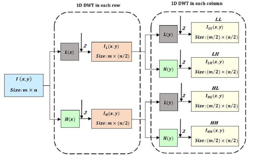
Figure 1. 2D-DWT single-level for I, which can be split into two stages. First, on each row of I, $(m\times n)$ is implemented and second intermediate subbands $[m\times(m/n)]$gain 1-DWT is implemented into two intermediate subbands.

Spatio-temporal data collection is a rapidly evolving field in which powerful computer processors (GPUs) for large-data analysis are used. Space-time databases contain data collected in a given place and time over both space and time that define an occurrence. A variety of spatio-temporal applications with rich details needs to convert LR images to HR images, such as target detection (Naqvi et al., 2020), recognition, and other high-resolution images (Deeba et al., 2021). Incorporated by a technology called super-resolution (SR), a number of researchers chose to reconstruct high-resolution (HR) images from low-resolution (LR) images instead of focusing on physical imaging (Deeba et al., 2020a). Ultimate spatio-temporal objects would be preserved and handled by a spatial database management system (SDBMS), which provides spatial capacities, including spatial data and operations models. The artifacts of space or time are not limited to 2D or 3D geometrical data. Spatio-temporal deep learning is becoming widely attractive and is essential to increase the resolution to retrieve the information from distinct applications such as GPS devices, internet-based map services, weather services, digital Earth, and satellite. The SISR is used to restore the high-resolution (HR) image in relation to the low-resolution (LR) issue (Deeba et al., 2020a) (Irani and Peleg, 1991) (Deeba et al., 2020b), given that the information on high frequencies must include HR images. Super-resolution can be commonly used in several applications, like medical imaging (Shi et al., 2013), satellite imaging (Thornton et al., 2006) (Dharejo et al., 2021), and health, safety, and monitoring (Zou and Yuen, 2011)(Nazir et al., 2020), where high-frequency requirements are quite relevant. SISR is a skewed problem, as it is appropriate to expect more HR pixels than the corresponding LR image (Yang et al., 2014). The example-based approach has been adapted to use this additional information by current methods, which either explore the self-similarities (Freedman and Fattal, 2011)(Yang et al., 2013), or map the LR counterpart in HR patches using external samples (Kim and Kwon, 2010)(Chang et al., 2004)(Timofte et al., 2013).

Further, to use sparse coding before assuming that an image might be a well-designed dictionary, the image will be a reasonable reference and is commonly used for sparse-code methods (Lu et al., 2013b)(Lu et al., 2013a). With the rapid growth of deep learning theory in recent years, deep neural networks have been widely used in various spatio-temporal remote sensing tasks; such as the remote sensing images scene-classification (Lu et al., 2017c), hyperspectral target image detection (Lu et al., 2017b), image classification (Lu et al., 2017a), and in multi spectral change detection (Zhang et al., 2018). Due to their good learning ability, DL-based methods have also been used to solve SR-based inverse problems, and the discovery of non-DL-based SR methods has been enhanced (Glasner et al., 2009)(Ma et al., 2019)(Dharejo et al., 2019)(Timofte et al., 2014). To significantly predict LR and HR image pairs nonlinear mapping, Dong et al. (Dong et al., 2014) uses CNNs and beats the non-DL-based SR methods.

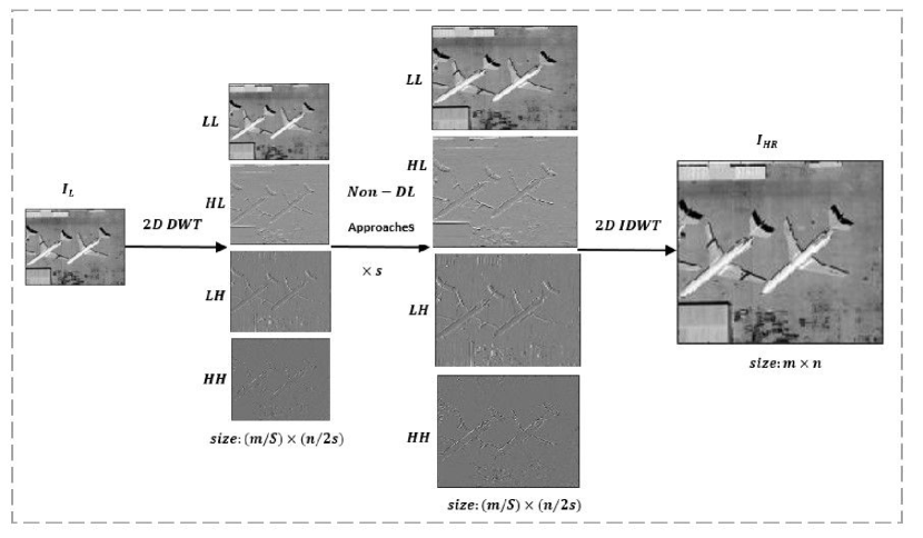
Figure 2. Flow chart of the method based on non-DL SR DWT. First, through the non-DL SR method, we decompose the LR image $I_{LR}$ into four wavelet components, and then increase the scale. Finally, combine the inverse 2-DWT operation as a super-resolution subband into the reconstructed HR image $I_{HR}$

Shi et al.(Shi et al., 2016) proposed a powerful CNN sub-pixel (ESPCN) that can minimize runtime by providing the LR image as input and preparing the network input HR image function map (rather than interpolating the LR version image). Dong et al. (Dong et al., 2016) proposed an accelerated lightweight network structure known as Super-Resolution Convolutional Neural Network (SRCNN). Kim et al. (Kim et al., 2016a) have shown a profound super-resolution network based on the achievement of highly deep networks (He et al., 2016) trained on ImageNet (Krizhevsky et al., 2017). They have used multiple HR and LR images with upgrade factors to minimize computation complexity speed up training. Kim et al. (Kim et al., 2016b) introduced more convolution layers to avoid adding a new parameter as the network depth was increased, and implemented the Deep Recurring Neural Network [DRCN]. Later the Deep Residual Network (DRRN) was proposed by Tai et al. (Tai et al., 2017), which attempts through residual learning, to build large but concise networks. As for the spatio-temporal remote sensing image resolution concerned, by using a generative model, Haut et al. (Haut et al., 2018) recognize image distribution and suggested a supervised method of SISR. Local and global residual learning (Lei et al., 2017) is incorporated into the reconstruction of supervised remote sensing images. Reconstruction with super-resolution can also help to distinguish hyperspectral images (Hao et al., 2018). Most existing SISR DL-based methods perform reconstructing the spatial domain and aim to increase LR pixels resolution and their HR image equivalents. In DL-based SISR strategies, this technique has been neglected, although it seems easier to restore missing high-frequency data within the frequency domain. Figure. 1 shows the single-level 2D-DWT method for $\boldsymbol{I}$, resulting in four subbands.

The wavelets have unique features, like sparse wavelet subbands; therefore, multi-scale modeling helps represent the image in better quality. Wavelet transform (WT) can extract information and perform multi-resolution analysis, often used in signal processing (Aballe et al., 1999)(Mallat and Hwang, 1992)(Abbate et al., 1995). The shift in wavelets has also been a very significant and efficient way for a multi-resolution image to be represented and stored (Mallat, 1996). It displays the spatial and textual details of the image on different levels. A wavelet method for compressing remote sensing images (Tian et al., 2011), a flexible Galerkin-Wavelet approach for restoring objects at a limited-angle tomography, is included in several remote sensing transformations (Lu et al., 2010). he wavelet transformation was widely adopted to support spatio-temporal imagery spatial resolution (Chan et al., 2003)(Kinebuchi et al., 2001)(Kim et al., 2007)(Li et al., 2010).The combination of wavelet transform and interpolation algorithm completes SR spatio-temporal remote sensing image task (Tao et al., 2003). Spatio-temporal remote sensing images data is acquired using our method from a multi-temporal and multi-viewpoint dataset, which can be considered a type of spatio-temporal remote sensing image. Non-redundant information can be obtained from a spatio-temporal remote-sensing image, enhancing useful information in the spatial domain and improving texture-feature representation. For this reason, it is an effective method for super-resolution reconstruction that utilizes the important information given by the spatio-temporal remote sensing image. As a result, the performance with which remote-sensing image data is used can be realistically enhanced. In this paper, a three-level super-resolution remote sensing image technique is proposed by combining transform wavelet and transferred generative adversarial networks detail enhancement based on spatio-temporal remote-sensing images. The first part incorporates the division in four subbands of the LR image through a 2-D discrete wavelet transform (DWT) and replacing the LR image with the low-frequency subband. Together the four subbands are inserted into the proposed network, as shown in Figure 4. Our proposed transmitted adversary network goal is to predict the residually improved HR wavelet component of the four corresponding sub-bands of single image super-resolution using basic generative adversarial network (SRGAN) architecture(Ledig et al., 2017). We mainly used the Transferred GAN to remove the redundant layers to decrease the memory burden and speed up the network. We train our model with an external data set DIV2K (Timofte et al., 2017) from previous knowledge of transfer learning and then fin-tune the network with remote sensing image datasets. Finally, by using the inverse 2D-IDWT transform, the HR reconstruction images are obtained. It is noticed that the network has become simpler by eliminating the redundant layers, and the computational network speed is much improved. Our paper has four main key contributions:

1. The proposed method is spatio-temporal remote sensing frequency-domain SISR to take full advantage of displaying images at different frequency bands (wavelet sub-bands).

2. The batch normalization layers are removed to minimize memory usage, processing burden, and enhance accuracy, unlike previous GAN-based SR approaches.

3. Our model is designed to cope with inadequate training in a transfer-learning way to implement deep learning techniques for spatio-temporal remote-sensing applications.

4. To further improve the performance, the low-frequency wavelet portion is replaced with a more accurate LR image. The results indicate that the proposed approach outperforms most state-of-the-art techniques to validate objective and subjective assessment accuracy.

The continuation of our paper is structured as Wavelet Transform (WT) details are in session II. The proposed approach is defined in session III. The experimental setup, qualitative, and quantitative analysis are in session IV, and they finally concluded in session V.

2. Background

We process the obtained spatio-temporal remote-sensing images in order to fully exploit complementary information between spatio-temporal remote-sensing images and create SR reconstruction images containing much detailed textures. We will briefly present the Wavelet Transform (WT) theory in this section and the conventional SISR approach based on DWT.

2.1. An Overview of Wavelet Transform

When the signal is decomposed in an ascending hierarchy, the wavelet transform collects time and frequency information (Li et al., 2006). The stable 1-D WT (1D-CWT) of the signal x(c) is given in equation (1),

(1) $$F(a,b)=\int_{-\infty}^{\infty}x(c)\psi_{a,b}(c)dc$$

Where $\psi_{a},_{b}(c)$ is the version of the mother wavelet dilated and translated as, environment.

(2) $$\psi_{a},_{b}(c)=\frac{1}{\sqrt{a}}\psi{\left(\frac{c-a}{b}\right)}$$

Where a and b are parameters for dilation regulation that regulate the Wavelet translation dilation. DWT is more proper to use to analyze discrete signals (Aha et al., 2005) instead of using the CWT. The $\leq x[d]$ discrete signal is set to 1D-DWT

(3) $$G(k,l)=\sum_{d=-\infty}^{\infty}x[d]\psi k,l(d)$$

Where $\psi k,l(d)$ the mother wavelet is dilated and translated version and can be measured as,

(4) $$\psi k,l(d)=2^{\frac{-k}{2}}\psi[2^{-k}d-l]$$

In reality, DWT would be used to transmit the input signal through the low-pass filter L(e) and high-pass filters H(e). Then to decrease its approximation and the accuracy of the input signal by 2 (Ledig et al., 2017). The Haar wavelets are defined as, L(e) and H(e),

(5) $$L(e)=\begin{cases}1,&e=0,1\\ 0,&otherwise\\ \end{cases}H(e)=\begin{cases}1,&e=0\\ -1,&e=0\\ 0,&otherwise\\ \end{cases}$$

For the 2-D image I, the pixel value of the xth and yth column should be indicated by I(x, y). 2D-DWT I is independently considered in each dimension accordingly; in columns and row sites, another term is used 1D-DWT. The 2D-DWT is divided into four substrates representing the average components; LL,LR, HL, HH.

2.2. SR Based on the Discrete Wavelet Transform (DWT)

The ability to properly reconstruct information is limited to interpolation-based SR methods. Since high-frequency domain information cannot be recovered well during SR, the result is not exact. Edges must be kept to increase super-resolved image performance. The DWT was used to maintain the image elements high frequency; for some of its high-frequency components, the $\boldsymbol{LL}$ portion with DWT decomposition, and the$\boldsymbol{LR}$, $\boldsymbol{HL}$ , and $\boldsymbol{HH}$ components are also structural data. DWT is combined with Non-DL SR methods by conventional DWT-based SR methods.

Let $I_{G}$ indicate the image of grounds truth HR in $m\times n$ by, and $I_{L}$ denote LR in size $\left(\frac{m}{s}\right)\times\left(\frac{n}{s}\right))$ by the same size (s), which is a scale factor. Allow the $\boldsymbol{I_{LR}}$ reflect LR up-scale performance, with m×n size, via bicubic interpolation, and $\boldsymbol{I_{HR}}$ to display the HR image reconstructed, with $\boldsymbol{m\times n}$ size.

1. Figure. 2 illustrates the DWT non-DL SR method’s flowchart, consisting of three steps; 2D-DWT, i.e., LL, HL, LH, and HH, decomposes IL into four separate subbands.

2. For each of the four subbands, a particular non-DL SR method is adopted for increasing their spatial resolution in s times.

3. The HR image of IHR is reconstructed, employing a discrete reverse WT (IDWT).

2.3. Generative Adversarial Networks

Generator G, which transforms a sample from a random uniform distribution to a given data, discriminator D, which calculates the probability of a sample being distributed by a data sample; (Dai et al., 2017) (GANs) is a two-characteristic class of data dispersion models. The game-theoretical min-max concepts are the origin of the generator and discriminator. They are usually taught in tandem by combining D and G instruction. Although GANs can visually attract images with high-frequency details, GANs still face many unanswered challenges, which means they are challenging to train. Recently, researchers have analyzed different aspects of GANs, such as the use of an accurate variable (Mirza and Osindero, 2014), training optimization (Salimans et al., 2016), and the use of task-specific cost functions (Creswell and Bharath, 2016). In addition, Shahin et al. (Mahdizadehaghdam et al., 2019) explore an alternative viewpoint on discrimination, which is different from the traditional view of probabilism as the paradigm of discrimination. In Figure 3, the most generic GAN architecture is given.

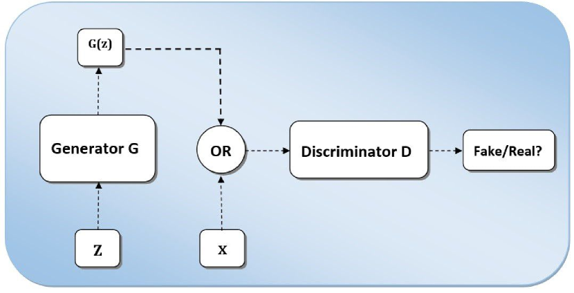
Figure 3. The general architecture of GAN.

3. Methodology

Once the corresponding wavelet elements are accurately predicted, high-quality HR images can be recovered from the LR image with comprehensive texture details and global topology information. Compared to CNN models, GANs have improved their performance and thus increased the quality of the image. GANs can enhance the consistency, appearance, and colour of images, build faces, and perform many more interesting tasks; GAN achieves good extraction and representation capacity. It thus can transform the reconstruction process of an HR image into the prediction of its wavelet portion. The two above facts allow us to put the TWIST-GAN schemes for the super-resolution challenge together with a GAN network and WT. The Figure.4 shows the entire architecture of Spatio-Temporal Remote Sensing Super-Resolution Combined with the Transferred Generative Adversarial Network and Wavelet Transformation (TWIST-GAN). It can be divided as the part disassembled, the part predicted, and the part reconstructed.

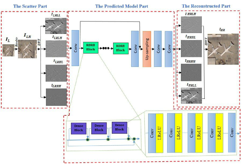
Figure 4. The method flow chart proposed by TWIST-GAN includes three parts; decompose parts, predict elements and reconstruct parts. The decomposed part decomposes the interpolated version of the LR image into four components of the LR wavelet. The prediction part uses a designed GAN-based SR network to estimate the LR counterpart’s HR wavelet component. 2D-IDWT is used to generate super-resolution images based on the HR wavelet components of the reconstructed part. The residual blocks are substituted with RRDB blocks. It is worth noting that RDDB contains dense blocks with ReLU and no BN layer.

3.1. Wavelet-based Scatter Part

Wavelet has various numerical methods that allow valuable information to be extracted from the signal and signals to be evaluated with different resolutions. Wavelet is an efficient multi-resolution solution for different imaging resolutions, such as high frequency and low-frequency images (Lu et al., 2017c)(Lu et al., 2017b)(Lu et al., 2017a)(Zhang et al., 2018). The image is separated into independent details by means of a wavelet transformation. The wavelet coefficients can be interpreted as vectors for the image. The high-frequency components can mirror the differences in the frequency in different directions to increase the texture detail. We train image coefficient wavelets to achieve the objective of reconstruction of remote sensing image super-resolution. Discrete packet wavelet decomposition and two-dimensional image reconstruction often used Haar wavelet as a wavelet base feature. It has a simple function, and the application is growing, particularly the reinforced symmetry that will allow us to avoid phase distortion during image decomposition.

We first obtain the ILR from the LR image IL for the first part that is disassembled. We decompose by using Haar wavelet decomposition into four wavelet components ILRLL, ILRLH, ILRHL, and ILRHH. From Figure. 2, Compared to IL, it can be seen that ILRLL has less detail, so we replaced the ILRLL component with IL, which is an input to the network that further helped boost the super-resolution quality. The disassembled part can be summarized as:

• Zoomed-in IL to obtain ILR using bicubic interpolation with a scale factor of ×s

• By sung 2D-DWT decomposition, ILR can be decomposed into ILRLL, ILRLH, ILRHL, and ILRHH.

• Load IL, ILRLH, ILRHL, and ILRHH into the GAN network that has been designed.

3.2. Predicted Model Part

The model TWIST-GAN with the structure provided in Figure.2 is used in the predicted portion to predict the wavelet components of the HR image from their LR counterparts, denoted by $\boldsymbol{I_{HRLL}},\boldsymbol{I_{HRLH}},\boldsymbol{I_{HRHL}},and\boldsymbol{I_{HRHH}}$. Alternatively, the SRGAN and proposed architectures are shown in Figure. 5(a,b), respectively. The batch normalization layers are omitted, providing more apparent evidence that the residual component batch normalization layers in the proposed architecture have been omitted. As indicated in EDSR (Dharejo et al., 2019), batch normalization (BN) layers are removed to decrease memory utilization and computational complexity. The entire TWIST-GAN network architecture is shown in Figure.4.

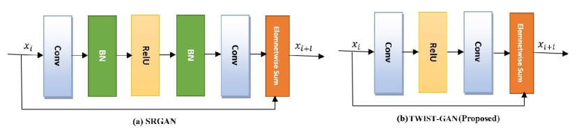
Figure 5. Comparison of the block architecture. (a) SRGAN’s block architecture (b) The proposed method’s block architecture.

In the same framework, we overlay a residual network in the generative network.The residual network’s core component is that the deep network can effectively control the generative model and reduce GAN preparation complexity. Recent research has developed residual high-performance networks for low and high-speed computer vision tasks. Although SRRes Net can be successfully implemented and deliver excellent efficiency in SRGAN, we work to simplify the network even further, although keeping good performance. To normalize the characteristics and reduce the heterogeneity (Lim et al., 2017), Nah et al. (Nah et al., 2017) have implemented the elimination of batch normalization layers from the network. However, the Batch Normalization (BN) layers are useful for the classification task, but the BN layers are not appropriate for the super-resolution task, as shown in Figure.5. As our strategic growth, the simplified network can display better image resolution performance than the original version. In addition, the batch normalization layers cost a lot of GPU memory and slow down the device rate. We can somewhat save about 43% of GPU memory during the workout and speed up running with our simplified version.

3.3. The Reconstruction Part

To reconstruct the HR super-resolved image IHR, we use a 2D-IDWT inverse wavelet onto four components $\boldsymbol{IHRLL},\boldsymbol{IHRLH},\boldsymbol{IHRHL},and\boldsymbol{IHRHH}.$

3.4. Network Architecture

We proposed TWIST-GAN by inspiring model SRGAN (Ledig et al., 2017), the configuration of the discriminator D is the same in our method as in SRGAN, but the G generator is changed to boost the SR outcome, as shown below:

1. The residual block is replaced by the residual-in-residual block called RDDB to use dense connections and multi-layer residual networks (Wang et al., 2018)

2. We have found from SRGAN that GAN suffers from training instability, so the original GAN is replaced with WGAN (Gulrajani et al., 2017) to resolve this deficiency. We are complementing G planning and helping to produce more realistic results.

3. From EDSR (Lim et al., 2017), we found that eliminating the layers of batch normalization can improve the network in terms of results and computation complexity.

RDDB can be defined as residual learning applied at different points to form a residual-in-residual (RDDB) structure. Short distances between a layer and each layer are built within each dense block; the block’s data flow could be linked. We use 25 RRBD blocks in our context. In addition to improving G architecture, BN layers are excluded. Removal of BN layers will bring several benefits. To eliminate the network complexity, BN-layers would first standardize the functionality. Secondly, BN layers consume extensive memory processing and GPU commonly. This can improve the network’s performance, particularly with limited computational resources, by removing batch normalization layers. When the network is very deep, and with an adversary’s learning (Wang et al., 2018), unnecessary artifacts may be added because of BN levels. For the above factors, the BN layer has been eliminated.

4. Experiment

4.1. Train the network via Transfer learning

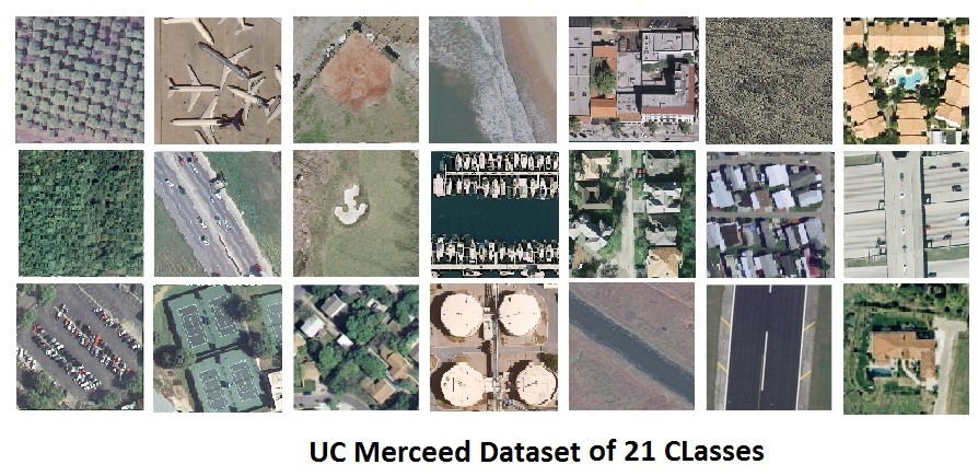
Figure 7. UC Merceed dataset uses 21 classes to evaluate our approach, and each class has 100 images with 256x256 pixel images.

The super-resolution of deep-learning spatio-temporal remote sensing images has more problems than the natural one. The research ideas of sufficiently strong samples are the foundation of deep learning. However, many high-quality satellite images that meet these criteria are not easy to obtain. Consequently, knowledge transfer from external data sets has received tremendous interest due to the continuous deep learning establishment. Transfer learning focuses on solving various problems in conjunction with areas using shared information, which leads to addressing tasks in an area based on experience gained from other environments. If only a few training samples are available, we may apply external knowledge through translation learning to the target domain.An external DIV2K dataset (Timofte et al., 2017) is used to prepare the proposed model in this paper. DIV2K is a contemporary image retrieval repository. There are 1,000 natural objects, all between 2000 and 1400 pixels, with a reasonable resolution. We prepare for the proposed model, especially, provide qualified training, and optimize the network. Participating images chosen from the objective datasets for the DIV2k training boost the per-trained network (Timofte et al., 2017). The pre-training network is optimized by obtaining images for training from the UC Merced dataset, a typical dataset of 256x256 pixel remote sensing image classification scenes, as shown in Figure.7. UC Merced contains a total of 21 natural images, with 100 images of each type. Finally, we choose the order targeting airplane and 80 airplane images as targets training samples, so the remaining 20 are used for testing. Figure.6 shows all the curves of performance grouped according to their respective test scales.

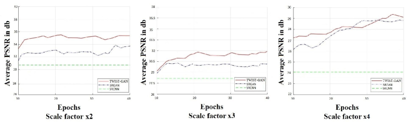
Figure 6. Concerning the progressively increased network depth, the output curves of the proposed TWIST-GAN on the UC Merceed dataset. As the test baselines, SRCNN and SRGAN are used. Note that SRCNN’s output will decrease with the increase in its depth, but we purposely fix the results to their corresponding peak values for better comparison. For SRGAN, for the sake of fairness, the experimental findings recorded in Figure 3are used directly.

4.2. Training Details

Above all, we explain the meaning of the relevant symbols. Let $\boldsymbol{X_{i}}$ represents the image of $\boldsymbol{ith}$ ground-truth HR $X_{i}-$, $X_{i-LH}$, $X_{i-HL}$, $X_{i-HH}$ denoting vector variants $\boldsymbol{X_{i}}$ wavelet components and $\hat{x}_{i}=[x_{i-}^{T},X_{i-LH}^{T},X_{i-HL}^{T},X_{i-HH}^{T}]^{T}$ denote how these components are concatenated. Similarly, for the reconstructed image, let $\boldsymbol{H_{i}}$ represents the $\boldsymbol{ith}$ reconstructed HR image. Where $x_{i}-,h_{i-LH},h_{i-HL},h_{i-HH}$ denoting vector variants of $H_{i}$ and h $\hat{h}_{i}=[h_{i-}^{T},h_{i-LH}^{T},h_{i-HL}^{T},h_{i-HH}^{T}]^{T}$ denote how these components are concatenated. In the training process, bicubic interpolation on 800 HR (down-sampling factor 2, 3, and 4) images have been used to obtain the LR image. During the Sub-image scale 256x256 training, the HR image is randomly trimmed into shape. The network reconstructs the image by learning the mapping relation between the LR image’s wavelet coefficients and the wavelet coefficients of the HR image. The network parameters are defined as the network learning rate is 0.0002, and the number of iterations is 28,000.
SISR task is to know a mapping function $X=gw(Y)$ between both the LR image $\boldsymbol{Y}$ and the HR image $\boldsymbol{X}$, where the network parameter is defined by $\boldsymbol{W}$. We measure the loss $\boldsymbol{l_{2}}$ of the wavelet components, different from other DL-based SR methods, the SR method measures the Euclidean distance between the real HR image and the reconstructed HR image as a loss. The technique to restore the real image and HR is as follows.

(6) $$loss=\frac{1}{N_{B}}\sum_{i=-1}^{N_{B}}\|\hat{x}_{i}-\hat{h}_{i}\|_{2}^{2}$$

Where $N_{B}$ refers to batch size. The proposed approach describes its overall objective function as,

(7) $$arg_{W}^{min}=\sum_{i=-1}^{N_{B}}\|\hat{x}_{i}-\hat{h}_{i}\|_{2}^{2}+\lambda\|\boldsymbol{W}\|_{2}^{2}$$

The first terminology is fidelity, meaning that the HR wavelet’s restored portion approximates the ground truth’s HR portion (Lu et al., 2013b). The second term is a regularization term to prevent overfitting, and the coefficient $\lambda$ is used to simplify the problem to simulate two terms together. The proposed approach is implemented in TensorFlow using a single 8-GB NVIDIA GTX1080 GPU, costing training five days and a day in relation and fine-tuning separately. We understand that our approach takes more time than SRCNN (Dong et al., 2016), VDSR (Kim and Kwon, 2010), and SRGAN (Ledig et al., 2017), DRCN (Kim et al., 2016a), respectively, for training. This is because the network we have designed is more complicated than the networks used in comparative approaches. However, the proposed method could yield better outcomes than the approaches compared.

(8) $$M(X,H)=\dfrac{1}{mn}\sum_{p=1}^{m}\sum_{q=1}^{n}(X(p,q)-H(p,q))^{2}$$

(9) $$PSNR(X,H)=10lg\frac{255^{2}}{MSE(X,H)}$$

Where m and n correspond to the image’s width and height, the larger the PSNR, the better quality image. Structure Similarity Index: To evaluate the structural similarity between the ground truth HR and the reconstructed HR image H, the Structural Similarity Index (SSIM) (Nah et al., 2017) is used, and defined as follows:

(10) $$SSIM(X,H)=l(X,H)c(X,H)s(X,H)$$

(11) $$l(X,H)=\frac{2\mu X\mu H+C_{1}}{\mu_{X}^{2}+\mu_{H}^{2}+C_{1}},c(X,H)=\frac{2\sigma X\sigma H+C_{2}}{\sigma_{X}^{2}+\sigma_{H}^{2}+C_{2}},s(X,H)=\frac{\sigma X\sigma H+C_{3}}{\sigma X\sigma H+C_{3}}$$

Where $\mu X$ and $\mu H$ express the mean value of $X$ and $H$, respectively, $\sigma X$ and $\sigma H$ show the standard deviation of $X$ and $H$, respectively, $\sigma XH$ is the covariance between $X$ and $H$, and $C_{1}$, $C_{2}$, and $C_{3}$ are constants. A higher SSIM value indicates superior quality.

4.3. Experimental results and analysis

We compared the research method with the SRGAN (Ledig et al., 2017) algorithm’s performance. On the training set DIV2K, we reproduced the suggested algorithm. The results of the SRGAN algorithm differ significantly from the test results since the different training sets. To assess the accuracy of the restored images with precision. In our method, we used PSNR, SSIM, FSIM, and UIQ as test indexes.Peak Signal-to-Noise Ratio (PSNR): The peak signal-to-noise ratio (PSNR) (Hore and Ziou, 2010) is an image quality measure and relies on the mean square error (MSE) between ground truth and the reconstructed image that can be expressed as:

Table 1. The PSNR value of HR reconstructed image (db) compared to the latest methods

Image	Scale	Bicubic	SRCNN	FSRCNN	ESPCN	VDSR	SRGAN	Proposed
			(Dong et al., 2014)	(Dong et al., 2016)	(Shi et al., 2016)	(Kim and Kwon, 2010)	(Ledig et al., 2017)	(TWIST-GAN)
airplane41	x2	28.56	31.88	33.01	32.78	34.14	34.18	35.15
	x3	25.66	28.13	29.47	29.19	30.27	30.36	31.23
	x4	24.12	25.97	26.21	25.22	27.24	27.45	28.28
airplane47	x2	29.16	30.89	32.12	33.07	34.43	34.33	34 .61
	x3	26.61	27.93	28.67	29.90	30.67	30.55	32.03
	x4	25.34	24.91	25.71	26.45	27.88	27.76	27.91
airplane90	x2	28.45	31.66	31.94	31.86	33.34	33.77	35.16
	x3	25.89	27.83	29.06	28.59	29.47	29.66	29.86
	x4	24.16	25.32	25.61	24.68	26.84	27.05	27.93
runway22	x2	27.24	30.11	30.39	31.19	33.38	33.68	34.25
	x3	24.16	27.13	28.07	28.59	29.46	29.96	31.01
	x4	23.82	23.17	24.81	25.32	26.49	26.95	27.18
Test Dataset	x2	32.16	32.98	33.81	34.08	34.26	34.31	35.21
(Zebra)	x3	28.32	29.13	30.49	31.14	31.79	30.76	31.10
	x4	27.02	28.95	29.01	29.22	29.29	29.41	29.83

Table 2. The SSIM value of HR reconstructed image compared to the latest methods

Image	Scale	Bicubic	SRCNN	FSRCNN	ESPCN	VDSR	SRGAN	Proposed
			(Dong et al., 2014)	(Dong et al., 2016)	(Shi et al., 2016)	(Kim et al., 2016a)	(Ledig et al., 2017)	(TWIST-GAN)
airplane41	x2	0.9156	0.9485	0.9521	0.9501	0.9537	0.9557	0.9607
	x3	0.8346	0.8764	0.8862	0.8831	0.8877	0.8979	0.9117
	x4	0.7672	0.8026	0.8165	0.8128	0.8189	0.8155	0.8607
airplane47	x2	0.9388	0.9596	0.9604	0.9589	0.9616	0.9625	0.9634
	x3	0.8616	0.8873	0.8911	0.8877	0.8961	0.8977	0.8987
	x4	0.7992	0.8133	0.8241	0.8185	0.8294	0.8319	0.8337
airplane90	x2	0.9142	0.9468	0.9512	0.9505	0.9529	0.9553	0.9587
	x3	0.8327	0.8735	0.8823	0.8811	0.8839	0.8956	0.8981
	x4	0.7672	0.8009	0.8119	0.8110	0.8231	0.8353	0.8391
runway22	x2	0.8786	0.9179	0.9231	0.9188	0.9310	0.9354	0.9401
	x3	0.7849	0.8254	0.8472	0.8352	0.8584	0.8631	0.9012
	x4	0.7132	0.7321	0.7525	0.7218	0.7618	0.7708	0.8417
Test Dataset	x2	0.9046	0.9322	0.9387	0.9373	0.9450	0.9527	0.9617
(Zebra)	x3	0.8126	0.8678	0.8705	0.8695	0.8789	0.8878	0.9123
	x4	0.7576	0.7916	0.8226	0.8213	0.8294	0.8514	0.8632

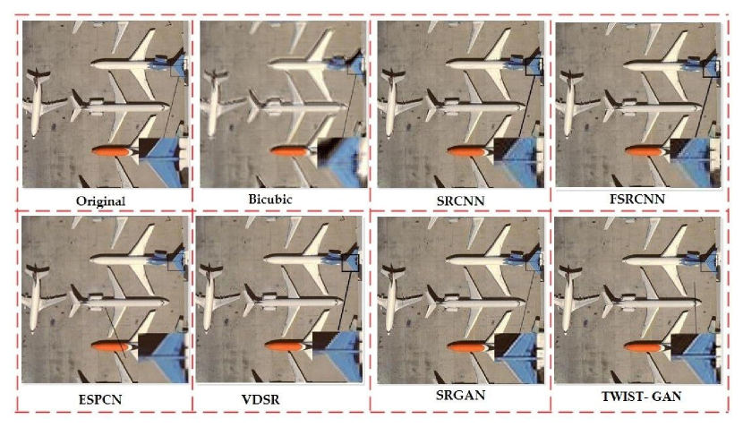
Figure 8. Comparison of reconstructed HR images of ”airplane 90.jpg” obtained from UCMerced LandUse dataset class ”airplane” with 256x256 pixel images using different methods with a scale factor of x2.

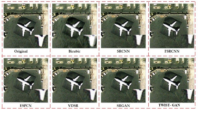
Figure 9. Comparison of reconstructed HR images of ”airplane 41.jpg” obtained from UCMerced LandUse dataset class ”airplane” with 256x256 pixel images using different methods with a scale factor of x2.

As shown in Figures. 8, 9, 10, 11, we evaluated our model on UCMerceed Landuse remote sensing dataset and also compared it with multiple methods, SRCNN dong01, FSRCNN dong02, EPCN shi01, VDSR kim01, and SRGAN lideg01. We also verify our outcome with the test dataset from set14, shown in Figure. 12. In visual as well as objective terms, the endorsed approach has been shown to perform better than all other strategies.We use FSIM and UIQ to evaluate the reconstructed image and analyze the details to evaluate the reconstructed image’s accuracy more effectively. Table. 3 and Table. 4 demonstrate the effects of our test images on FSI Mand UIQ. The better the restored image’s quality, the closer the value of FSIM and UIQ is to 1. We propose a wavelet and GAN-based super-resolution reconstruction algorithm to enhance the restored image and HR image generation’s objective evaluation with a richer texture.

Table 3. The FSIM value of HR reconstructed image compared to the latest methods

Image	Scale	Bicubic	SRCNN	FSRCNN	ESPCN	VDSR	SRGAN	Proposed
			(Dong et al., 2014)	(Dong et al., 2016)	(Shi et al., 2016)	(Kim et al., 2016a)	(Ledig et al., 2017)	(TWIST-GAN)
airplane41	x2	0.896	0.935	0.942	0.937	0.948	0.952	0.965
	x3	0.814	0.878	0.879	0.877	0.896	0.907	0.917
	x4	0.757	0.807	0.815	0.808	0.825	0.834	0.852
airplane47	x2	0.902	0.938	0.943	0.931	0.946	0.951	0.954
	x3	0.825	0.884	0.888	0.879	0.893	0.906	0.913
	x4	0.769	0.819	0.826	0.817	0.837	0.838	0.847
airplane90	x2	0.889	0.931	0.940	0.933	0.944	0.948	0.959
	x3	0.809	0.874	0.875	0.872	0.893	0.903	0.912
	x4	0.752	0.803	0.812	0.804	0.821	0.830	0.848
runway22	x2	0.881	0.918	0.924	0.917	0.928	0.927	0.933
	x3	0.807	0.853	0.861	0.860	0.867	0.892	0.907
	x4	0.735	0.799	0.807	0.802	0.817	0.821	0.849
Test Dataset	x2	0.892	0.931	0.938	0.931	0.942	0.948	0.951
(Zebra)	x3	0.812	0.874	0.882	0.872	0.891	0.902	0.912
	x4	0.754	0.802	0.819	0.797	0.821	0.829	0.847

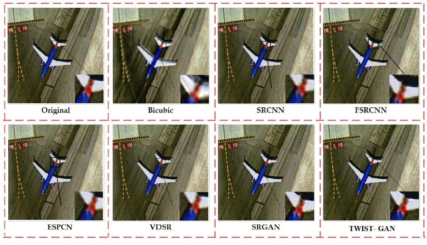
Figure 10. Comparison of reconstructed HR images of ”airplane 47.jpg” obtained from UCMerced LandUse dataset class ”airplane” with 256x256 pixel images using different methods with a scale factor of x2.

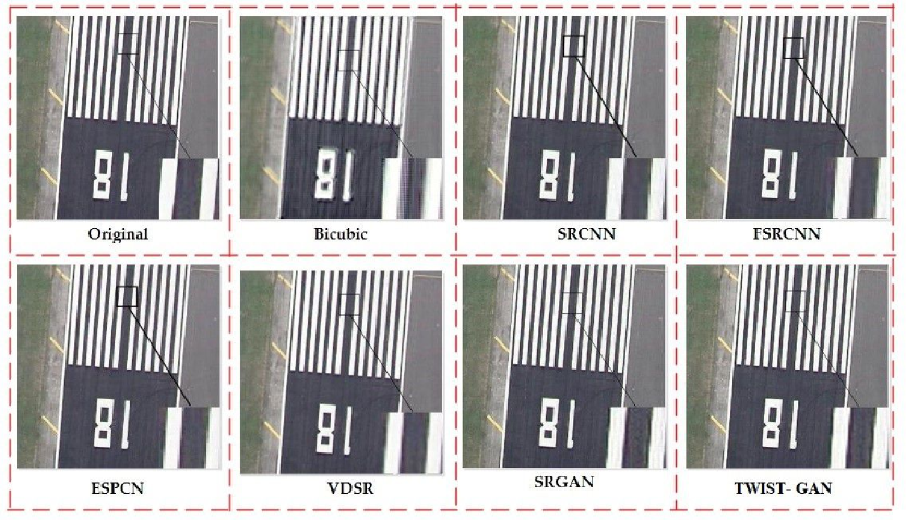
Figure 11. Comparison of reconstructed HR images of ”runway 22.jpg” obtained from UCMerced LandUse dataset class ”runway” with 256x256 pixel images using different methods with a scale factor of x2.

Table 4. The UIQ value of HR reconstructed image compared to the latest methods

Image	Scale	Bicubic	SRCNN	FSRCNN	ESPCN	VDSR	SRGAN	Proposed
			(Dong et al., 2014)	(Dong et al., 2016)	(Shi et al., 2016)	(Kim et al., 2016a)	(Ledig et al., 2017)	(TWIST-GAN)
airplane41	x2	0.889	0.928	0.932	0.931	0.938	0.948	0.957
	x3	0.808	0.865	0.867	0.866	0.893	0.902	0.914
	x4	0.749	0.798	0.806	0.802	0.819	0.830	0.848
airplane47	x2	0.901	0.929	0.935	0.931	0.941	0.948	0.950
	x3	0.818	0.872	0.881	0.875	0.891	0.902	0.911
	x4	0.755	0.817	0.823	0.814	0.833	0.834	0.844
airplane90	x2	0.883	0.926	0.930	0.928	0.937	0.939	0.943
	x3	0.805	0.861	0.866	0.865	0.873	0.896	0.905
	x4	0.748	0.796	0.804	0.797	0.807	0.826	0.839
runway22	x2	0.887	0.916	0.922	0.915	0.925	0.924	0.929
	x3	0.805	0.851	0.860	0.858	0.864	0.890	0.904
	x4	0.746	0.796	0.804	0.799	0.814	0.818	0.843
Test Dataset	x2	0.888	0.917	0.925	0.916	0.927	0.926	0.932
(Zebra)	x3	0.807	0.855	0.862	0.859	0.866	0.893	0.906
	x4	0.747	0.799	0.807	0.803	0.818	0.820	0.846

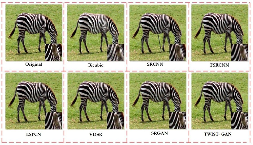
Figure 12. Comparison of reconstructed HR images of ”freeway 39.jpg” obtained from set14 dataset class ”zebra” with resized 256x256 pixel images using different methods with a scale factor of x2.

The run-time of all algorithms is illustrated in Table. 5. The running time of the conventional algorithm is longer than that of the deep learning algorithms. Bicubic shows the shortest time-consuming because it only has interpolation operations. SRCNN and VDS take a longer time between LR and HR image patch pairs. SRGAN and ESPCN models have a wide range of convolutional layers, so they all take a long time to train TWIST-GAN to reduce network depth by eliminating BN layers and not increasing network time complexity. Although FSRCNN performs better, it does not perform well in visual quality, such as PSNR and SSIM. We performed experiments with the same hardware setup, and carried out all algorithms: Intel Core i7-6700K C3.20 GHz CPU via an NVIDIA GTX1080 GPU 8 GB RAM.

Table 5. Total running time of different algorithms on UCMerced dataset.

Algorithms	Bicubic	SRCNN	FSRCNN	ESPCN	VDSR	SRGAN	Proposed
		(Dong et al., 2014)	(Dong et al., 2016)	(Shi et al., 2016)	(Kim et al., 2016a)	(Ledig et al., 2017)	(TWIST-GAN)
Running/Time	10.269	15.144	12.025	14.301	17.442	16.278	13.935

4.4. Model Convergence

Our TWIST-GAN improves SRGAN by training multiple networks to characterize wavelets. We compare their training convergence speeds. The experiments are carried out in the same network setup and computing environment. The curves of convergence regarding PSNR are shown in Figure.13. Within 8 to 104of the SRGAN is converged to our TWIST-GAN optima with better accuracy of 4 to 104iterations. TWIST-GAN restores the entire aerial image straight away, and transfers the whole aerial image.

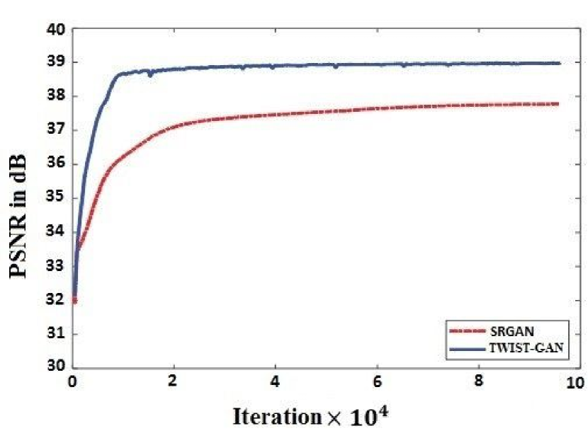
Figure 13. Comparison of reconstructed HR images of ”freeway 39.jpg” obtained from set14 dataset class ”zebra” with resized 256x256 pixel images using different methods with a scale factor of x2.

5. CONCLUSION

We propose a method to provide the super-resolution performance of remote sensing images by wavelet transformation and transferred generative adversarial network. The computational cost of our approach is minimized, and the similarity of spatio-temporal remote-sensing data is increased by preprocessing spatio-temporal remote-sensing data. The method is validated by several sets of experiments conducted on common remote sensing data. We first trained our network on the high-resolution DIV2K dataset, and then applied transfer learning techniques to train and test the remote sensing images on the UC Merceed dataset. The objective and subjective results demonstrate the significance of our proposed approach. The experimental results suggest that the proposed method can effectively develop the objective assessment limitations, and the reconstructed images are more realistic images with more texture details. This demonstrates that our proposed algorithm got the advantage of wavelet packet transformation and Transfer GAN in spatio-temporal remote sensing image super-resolution. Although the proposed method is effective, it can still be improved by applying other techniques in future work, such as multi-resolution discrete wavelet transform and dual-tree complex wavelet transform. High-frequency data from natural image data sets can be extracted using these techniques.

6. Acknowledgments

This work was supported in part by the Key Research Program of Frontier Sciences, CAS, and Grant number ZDBS-LY-DQC016, Beijing Natural Science Foundation under Grant No. 4212030, Beijing Nova Program of Science and Technology under Grant No. Z191100001119090, Natural Science Foundation of China under Grant No. 61836013 and, Youth Innovation Promotion Association CAS.

References

- (1)
- Aballe et al. (1999) A Aballe, M Bethencourt, FJ Botana, and M Marcos. 1999. Using wavelets transform in the analysis of electrochemical noise data. Electrochimica Acta 44, 26 (1999), 4805–4816.
- Abbate et al. (1995) A Abbate, J Frankel, and P Das. 1995. Wavelet transform signal processing for dispersion analysis of ultrasonic signals. In 1995 IEEE Ultrasonics Symposium. Proceedings. An International Symposium, Vol. 1. IEEE, Seattle, WA, USA, 751–755.
- Aha et al. (2005) David W Aha, David McSherry, and Qiang Yang. 2005. Advances in conversational case-based reasoning. The knowledge engineering review 20, 3 (2005), 247.
- Chan et al. (2003) Raymond H Chan, Tony F Chan, Lixin Shen, and Zuowei Shen. 2003. Wavelet algorithms for high-resolution image reconstruction. SIAM Journal on Scientific Computing 24, 4 (2003), 1408–1432.
- Chang et al. (2004) Hong Chang, Dit-Yan Yeung, and Yimin Xiong. 2004. Super-resolution through neighbor embedding. In Proceedings of the 2004 IEEE Computer Society Conference on Computer Vision and Pattern Recognition, 2004. CVPR 2004., Vol. 1. IEEE, Washington, DC, USA, I–I.
- Creswell and Bharath (2016) Antonia Creswell and Anil A Bharath. 2016. Task specific adversarial cost function. arXiv preprint arXiv:1609.08661 abs/1609.08661 (2016), 0–0.
- Dai et al. (2017) Guoxian Dai, Jin Xie, and Yi Fang. 2017. Metric-based generative adversarial network. In Proceedings of the 25th ACM international conference on Multimedia. ACM, Mountain View, California, USA, 672–680.
- Deeba et al. (2020a) Farah Deeba, She Kun, Fayaz Ali Dharejo, and Yuanchun Zhou. 2020a. Sparse representation based computed tomography images reconstruction by coupled dictionary learning algorithm. IET Image Processing 14, 11 (2020), 2365–2375.
- Deeba et al. (2020b) Farah Deeba, She Kun, Fayaz Ali Dharejo, and Yuanchun Zhou. 2020b. Wavelet-Based Enhanced Medical Image Super Resolution. IEEE Access 8 (2020), 37035–37044.
- Deeba et al. (2021) Farah Deeba, Yuanchun Zhou, Fayaz Ali Dharejo, Muhammad Ashfaq Khan, Bhagwan Das, Xuezhi Wang, and Yi Du. 2021. A plexus-convolutional neural network framework for fast remote sensing image super-resolution in wavelet domain. IET Image Processing 0, 0 (2021), 0–0.
- Dharejo et al. (2019) Fayaz Ali Dharejo, Yuanchun Zhou, Farah Deeba, and Yi Du. 2019. A color enhancement scene estimation approach for single image haze removal. IEEE Geoscience and Remote Sensing Letters 17, 9 (2019), 1613–1617.
- Dharejo et al. (2021) Fayaz Ali Dharejo, Yuanchun Zhou, Farah Deeba, Munsif Ali Jatoi, Yi Du, and Xuezhi Wang. 2021. A remote-sensing image enhancement algorithm based on patch-wise dark channel prior and histogram equalisation with colour correction. IET image Processing 15, 1 (2021), 47–56.
- Dong et al. (2014) Chao Dong, Chen Change Loy, Kaiming He, and Xiaoou Tang. 2014. Learning a deep convolutional network for image super-resolution. In European conference on computer vision. Springer, Zurich, Switzerland, 184–199.
- Dong et al. (2016) Chao Dong, Chen Change Loy, and Xiaoou Tang. 2016. Accelerating the super-resolution convolutional neural network. In European conference on computer vision. Springer, Amsterdam, Netherlands, 391–407.
- Freedman and Fattal (2011) Gilad Freedman and Raanan Fattal. 2011. Image and video upscaling from local self-examples. ACM Transactions on Graphics (TOG) 30, 2 (2011), 1–11.
- Glasner et al. (2009) Daniel Glasner, Shai Bagon, and Michal Irani. 2009. Super-resolution from a single image. In 2009 IEEE 12th international conference on computer vision. IEEE, Kyoto, Japan, 349–356.
- Gulrajani et al. (2017) Ishaan Gulrajani, Faruk Ahmed, Martin Arjovsky, Vincent Dumoulin, and Aaron Courville. 2017. Improved training of wasserstein gans. arXiv preprint arXiv:1704.00028 0, 0 (2017), 0–0.
- Hanif et al. (2020) Muhammad Hanif, Rizwan Ali Naqvi, Sagheer Abbas, Muhammad Adnan Khan, and Nadeem Iqbal. 2020. A Novel and Efficient 3D Multiple Images Encryption Scheme Based on Chaotic Systems and Swapping Operations. IEEE Access 8 (2020), 123536–123555.
- Hao et al. (2018) Siyuan Hao, Wei Wang, Yuanxin Ye, Enyu Li, and Lorenzo Bruzzone. 2018. A deep network architecture for super-resolution-aided hyperspectral image classification with classwise loss. IEEE Transactions on Geoscience and Remote Sensing 56, 8 (2018), 4650–4663.
- Haut et al. (2018) Juan Mario Haut, Ruben Fernandez-Beltran, Mercedes E Paoletti, Javier Plaza, Antonio Plaza, and Filiberto Pla. 2018. A new deep generative network for unsupervised remote sensing single-image super-resolution. IEEE Transactions on Geoscience and Remote sensing 56, 11 (2018), 6792–6810.
- He et al. (2016) Kaiming He, Xiangyu Zhang, Shaoqing Ren, and Jian Sun. 2016. Deep residual learning for image recognition. In Proceedings of the IEEE conference on computer vision and pattern recognition. IEEE, Las Vegas, NV, USA, 770–778.
- Hore and Ziou (2010) Alain Hore and Djemel Ziou. 2010. Image quality metrics: PSNR vs. SSIM. In 2010 20th international conference on pattern recognition. IEEE, Istanbul, Turkey, 2366–2369.
- Irani and Peleg (1991) Michal Irani and Shmuel Peleg. 1991. Improving resolution by image registration. CVGIP: Graphical models and image processing 53, 3 (1991), 231–239.
- Kim et al. (2016a) Jiwon Kim, Jung Kwon Lee, and Kyoung Mu Lee. 2016a. Accurate image super-resolution using very deep convolutional networks. In Proceedings of the IEEE conference on computer vision and pattern recognition. IEEE, Las Vegas, NV, USA, 1646–1654.
- Kim et al. (2016b) Jiwon Kim, Jung Kwon Lee, and Kyoung Mu Lee. 2016b. Deeply-recursive convolutional network for image super-resolution. In Proceedings of the IEEE conference on computer vision and pattern recognition. IEE, Las Vegas, NV, USA, 1637–1645.
- Kim and Kwon (2010) Kwang In Kim and Younghee Kwon. 2010. Single-image super-resolution using sparse regression and natural image prior. IEEE transactions on pattern analysis and machine intelligence 32, 6 (2010), 1127–1133.
- Kim et al. (2007) Sang Soo Kim, II Kyu Eom, and Yoo Shin Kim. 2007. Image interpolation based on statistical relationship between wavelet subbands. In 2007 IEEE International Conference on Multimedia and Expo. IEEE, Beijing, China, 1723–1726.
- Kinebuchi et al. (2001) Kentaro Kinebuchi, D Darian Muresan, and Thomas W Parks. 2001. Image interpolation using wavelet based hidden Markov trees. In 2001 IEEE International Conference on Acoustics, Speech, and Signal Processing. Proceedings (Cat. No. 01CH37221), Vol. 3. IEEE, Salt Lake City, UT, USA, 1957–1960.
- Krizhevsky et al. (2017) Alex Krizhevsky, Ilya Sutskever, and Geoffrey E Hinton. 2017. ImageNet classification with deep convolutional neural networks. Commun. ACM 60, 6 (2017), 84–90.
- Ledig et al. (2017) Christian Ledig, Lucas Theis, Ferenc Huszár, Jose Caballero, Andrew Cunningham, Alejandro Acosta, Andrew Aitken, Alykhan Tejani, Johannes Totz, Zehan Wang, et al. 2017. Photo-realistic single image super-resolution using a generative adversarial network. In Proceedings of the IEEE conference on computer vision and pattern recognition. IEEE, Honolulu, HI, USA, 4681–4690.
- Lei et al. (2017) Sen Lei, Zhenwei Shi, and Zhengxia Zou. 2017. Super-resolution for remote sensing images via local–global combined network. IEEE Geoscience and Remote Sensing Letters 14, 8 (2017), 1243–1247.
- Li et al. (2010) Bo Li, Rui Yang, and Hongxu Jiang. 2010. Remote-sensing image compression using two-dimensional oriented wavelet transform. IEEE Transactions on Geoscience and Remote sensing 49, 1 (2010), 236–250.
- Li et al. (2006) Xueke Li, Xiaolin Tian, Yankui Sun, and Zesheng Tang. 2006. Medical image fusion by multi-resolution analysis of wavelets transform. In Wavelet Analysis and Applications. Springer, -, 389–396.
- Lim et al. (2017) Bee Lim, Sanghyun Son, Heewon Kim, Seungjun Nah, and Kyoung Mu Lee. 2017. Enhanced deep residual networks for single image super-resolution. In Proceedings of the IEEE conference on computer vision and pattern recognition workshops. IEEE, Honolulu, HI, USA, 136–144.
- Lu et al. (2010) Xiaoqiang Lu, Yi Sun, and Gangfeng Bai. 2010. Adaptive wavelet-Galerkin methods for limited angle tomography. Image and Vision Computing 28, 4 (2010), 696–703.
- Lu et al. (2017a) Xiaoqiang Lu, Binqiang Wang, Xiangtao Zheng, and Xuelong Li. 2017a. Exploring models and data for remote sensing image caption generation. IEEE Transactions on Geoscience and Remote Sensing 56, 4 (2017), 2183–2195.
- Lu et al. (2013a) Xiaoqiang Lu, Yuan Yuan, and Pingkun Yan. 2013a. Alternatively constrained dictionary learning for image superresolution. IEEE Transactions on Cybernetics 44, 3 (2013), 366–377.
- Lu et al. (2013b) Xiaoqiang Lu, Yuan Yuan, and Pingkun Yan. 2013b. Image super-resolution via double sparsity regularized manifold learning. IEEE transactions on circuits and systems for video technology 23, 12 (2013), 2022–2033.
- Lu et al. (2017b) Xiaoqiang Lu, Wuxia Zhang, and Xuelong Li. 2017b. A hybrid sparsity and distance-based discrimination detector for hyperspectral images. IEEE Transactions on Geoscience and Remote Sensing 56, 3 (2017), 1704–1717.
- Lu et al. (2017c) Xiaoqiang Lu, Xiangtao Zheng, and Yuan Yuan. 2017c. Remote sensing scene classification by unsupervised representation learning. IEEE Transactions on Geoscience and Remote Sensing 55, 9 (2017), 5148–5157.
- Ma et al. (2019) Wen Ma, Zongxu Pan, Jiayi Guo, and Bin Lei. 2019. Achieving super-resolution remote sensing images via the wavelet transform combined with the recursive res-net. IEEE Transactions on Geoscience and Remote Sensing 57, 6 (2019), 3512–3527.
- Mahdizadehaghdam et al. (2019) Shahin Mahdizadehaghdam, Ashkan Panahi, and Hamid Krim. 2019. Sparse generative adversarial network. In Proceedings of the IEEE/CVF International Conference on Computer Vision Workshops. IEEE, Seoul, Korea (South), 0–0.
- Mallat (1996) Stephane Mallat. 1996. Wavelets for a vision. Proc. IEEE 84, 4 (1996), 604–614.
- Mallat and Hwang (1992) Stephane Mallat and Wen Liang Hwang. 1992. Singularity detection and processing with wavelets. IEEE transactions on information theory 38, 2 (1992), 617–643.
- Mirza and Osindero (2014) Mehdi Mirza and Simon Osindero. 2014. Conditional generative adversarial nets. arXiv preprint arXiv:1411.1784 0, o (2014), 0–0.
- Nah et al. (2017) Seungjun Nah, Tae Hyun Kim, and Kyoung Mu Lee. 2017. Deep multi-scale convolutional neural network for dynamic scene deblurring. In Proceedings of the IEEE conference on computer vision and pattern recognition. IEEE, Honolulu, HI, USA, 3883–3891.
- Naqvi et al. (2020) Rizwan Ali Naqvi, Muhammad Arsalan, Abdul Rehman, Ateeq Ur Rehman, Woong-Kee Loh, and Anand Paul. 2020. Deep learning-based drivers emotion classification system in time series data for remote applications. Remote Sensing 12, 3 (2020), 587.
- Nazir et al. (2020) Tahira Nazir, Aun Irtaza, Ali Javed, Hafiz Malik, Dildar Hussain, and Rizwan Ali Naqvi. 2020. Retinal Image Analysis for Diabetes-Based Eye Disease Detection Using Deep Learning. Applied Sciences 10, 18 (2020), 6185.
- Salimans et al. (2016) Tim Salimans, Ian Goodfellow, Wojciech Zaremba, Vicki Cheung, Alec Radford, and Xi Chen. 2016. Improved techniques for training gans. arXiv preprint arXiv:1606.03498 0, 0 (2016), 0–0.
- Shi et al. (2016) Wenzhe Shi, Jose Caballero, Ferenc Huszár, Johannes Totz, Andrew P Aitken, Rob Bishop, Daniel Rueckert, and Zehan Wang. 2016. Real-time single image and video super-resolution using an efficient sub-pixel convolutional neural network. In Proceedings of the IEEE conference on computer vision and pattern recognition. IEEE, Las Vegas, NV, USA, 1874–1883.
- Shi et al. (2013) Wenzhe Shi, Jose Caballero, Christian Ledig, Xiahai Zhuang, Wenjia Bai, Kanwal Bhatia, Antonio M Simoes Monteiro de Marvao, Tim Dawes, Declan O’Regan, and Daniel Rueckert. 2013. Cardiac image super-resolution with global correspondence using multi-atlas patchmatch. In International conference on medical image computing and computer-assisted intervention. Springer, Nagoya, Japan, 9–16.
- Tai et al. (2017) Ying Tai, Jian Yang, and Xiaoming Liu. 2017. Image super-resolution via deep recursive residual network. In Proceedings of the IEEE conference on computer vision and pattern recognition. IEE, Honolulu, HI, USA, 3147–3155.
- Tao et al. (2003) Hongjiu Tao, Xinjian Tang, Jian Liu, and Jinwen Tian. 2003. Superresolution remote sensing image processing algorithm based on wavelet transform and interpolation. In Image Processing and Pattern Recognition in Remote Sensing, Vol. 4898. International Society for Optics and Photonics, Hangzhou, China, 259–263.
- Thornton et al. (2006) Matt W Thornton, Peter M Atkinson, and DA Holland. 2006. Sub-pixel mapping of rural land cover objects from fine spatial resolution satellite sensor imagery using super-resolution pixel-swapping. International Journal of Remote Sensing 27, 3 (2006), 473–491.
- Tian et al. (2011) Jing Tian, Lihong Ma, and Weiyu Yu. 2011. Ant colony optimization for wavelet-based image interpolation using a three-component exponential mixture model. Expert Systems with Applications 38, 10 (2011), 12514–12520.
- Timofte et al. (2017) Radu Timofte, Eirikur Agustsson, Luc Van Gool, Ming-Hsuan Yang, and Lei Zhang. 2017. Ntire 2017 challenge on single image super-resolution: Methods and results. In Proceedings of the IEEE conference on computer vision and pattern recognition workshops. IEEE, Honolulu, HI, USA, 114–125.
- Timofte et al. (2013) Radu Timofte, Vincent De Smet, and Luc Van Gool. 2013. Anchored neighborhood regression for fast example-based super-resolution. In Proceedings of the IEEE international conference on computer vision. IEEE, Sydney, NSW, Australia, 1920–1927.
- Timofte et al. (2014) Radu Timofte, Vincent De Smet, and Luc Van Gool. 2014. A+: Adjusted anchored neighborhood regression for fast super-resolution. In Asian conference on computer vision. Springer, Singapore, Singapore, 111–126.
- Wang et al. (2018) Xintao Wang, Ke Yu, Shixiang Wu, Jinjin Gu, Yihao Liu, Chao Dong, Yu Qiao, and Chen Change Loy. 2018. Esrgan: Enhanced super-resolution generative adversarial networks. In Proceedings of the European Conference on Computer Vision (ECCV) Workshops. Springier, Munich, Germany, 0–0.
- Yang et al. (2014) Chih-Yuan Yang, Chao Ma, and Ming-Hsuan Yang. 2014. Single-image super-resolution: A benchmark. In European conference on computer vision. Springer, Zurich, Switzerla, 372–386.
- Yang et al. (2013) Jianchao Yang, Zhe Lin, and Scott Cohen. 2013. Fast image super-resolution based on in-place example regression. In Proceedings of the IEEE conference on computer vision and pattern recognition. IEEE, Portland, OR, USA, 1059–1066.
- Zhang et al. (2018) Wuxia Zhang, Xiaoqiang Lu, and Xuelong Li. 2018. A coarse-to-fine semi-supervised change detection for multispectral images. IEEE Transactions on Geoscience and Remote Sensing 56, 6 (2018), 3587–3599.
- Zou and Yuen (2011) Wilman WW Zou and Pong C Yuen. 2011. Very low resolution face recognition problem. IEEE Transactions on image processing 21, 1 (2011), 327–340.