Variance Reduction of Quadcopter Trajectory Tracking in Turbulent Wind

Abstract

We consider a quadcopter operating in a turbulent windy environment. The turbulent environment may be imposed on a quadcopter by structures, landscapes, terrains and most importantly by the unique physical phenomena in the lower atmosphere. Turbulence can negatively impact quadcopter’s performance and operations. Modeling turbulence as a stochastic random input, we investigate control designs that can reduce the turbulence effects on the quadcopter’s motion. In particular, we design a minimum cost variance (MCV) controller aiming to minimize the cost in terms of its weighted sum of mean and variance. We linearize the quadcopter dynamics and examine the MCV controller derived from a set of coupled algebraic Riccati equations (CARE) with full-state feedback. Our preliminary simulation results show reduction in variance and in mean trajectory tracking error compared to a traditional linear quadratic regulator (LQR).

1 Introduction

Small Unmanned Aircraft System (sUAS) has become ubiquitous in diverse applications and are aggressively being integrated into the national airspace system (NAS). Multi-rotor platforms such as quadcopters have demonstrated significant potentials in small package delivery, surveillance operations and in many other applications. Many of the tasks involve operations in the low-altitude airspace. In the urban setting low-altitude operations impose challenges to operational and navigational tasks with its unique physical phenomena. Being under-actuated, a quadcopter is vulnerable to strong mean wind velocity as well as unsteady wind gusts. Gill and D’Andrea (2017) show that with a relative wind velocity more than $4-7ms^{-1}$, the hover model of a quadcopter deteriorates.

To compensate for the wind effects, several disturbance rejection algorithms have been studied. Some of them require wind information, onboard wind estimation or prediction while others solve optimal policy without any wind information. Tran et al. (2015) illustrate the performance of the traditional PID and LQR controllers for disturbance rejection where an offline computed look-up table is used to estimate wind components in the simulation. Wang et al. (2016) propose a hierarchical nonlinear control scheme for a quadcopter to track a 3D trajectory subject to wind gust disturbances from a von Karman model. In Zhang et al. (2016), a three-dimensional fuzzy PID control method for stabilizing attitude control and precise trajectory tracking control is implemented with wind gusts generated from a Dryden model in the simulation. Yang et al. (2017) investigate attitude control via a dual closed-loop control framework where gust wind is considered dynamic disturbances and estimated by an extended state observer. Ding and Wang (2018) propose a linear active disturbance rejection control (LADRC) for stability control of a quadcopter under wind gusts with a linear extended state observer (LESO) as a compensator. A geometric adaptive controller is proposed in Bisheban and Lee (2018) and a numerical example is illustrated. An adaptive mass estimator and an adaptive neural disturbance estimator are derived in Sierra and Santos (2019) that complement the action of a set of PID controllers stabilizing a sUAS under wind and variable payload. A second order sliding mode controller based on the super twisting algorithm (STA) with an observer is employed in Hamadi et al. (2019) to reject wind perturbation. A real-time simulation study in wind is provided in Davoudi et al. (2020). Tran et al. (2021) introduce Particle Swarm Optimisation (PSO) based Adaptive Strictly Negative Imaginary (SNI) controller for unknown wind disturbance rejection.

Almost every controller in the literature developed for wind disturbance rejection is focused on reducing the mean of the tracking error. In this paper, our objective is to incorporate stochastic properties of wind into a controller and reduce the variance of tracking error, which, to the best of the authors’ knowledge, has not been considered in previous research. In particular, we introduce a Minimum Cost Variance controller (Sain (1965)) which is a special case of risk sensitive control (Sain et al. (1995)) in the quadcopter control paradigm. We consider a quadcopter model including a body drag effect and a stochastic differential dynamic model to assimilate the stochastic property of the wind. Previous studies except Davoudi et al. (2020) have not considered a realistic lower atmospheric conditions. Davoudi et al. (2020) is mostly focused on the realistic flight simulation in the wind field. Here, we adopt Large-Eddy Simulations to obtain high-fidelity Atmospheric Boundary Layer wind solutions and extract stochastic information. In the MCV formulation, the standard deviation of the wind information is incorporated into the stochastic model and an optimal controller is obtained to optimize the weighted sum of the mean and the variance of the cost. To generate a MCV controller for quadcopter trajectory tracking, we linearize the quadcopter dynamics along a planned trajectory and create a finite-horizon MCV controller based on the linearized model. We simulate hover, straight line and circular trajectories with the LES wind data to examine the effectiveness of the controller. In each case, we compare the MCV controller with an LQR controller and find that the MCV controller produces reduced turbulent effects and tracking error.

The rest of the paper is structured as follows. Section  2 discusses the mathematical models of the wind and the quadcopter dynamics used for controller designs. In Section 3 we present our controller design. We discuss the simulation results in Section 4. Future work is summarized in Section 5.

2 Mathematical Model

2.1 Modeling Atmospheric Wind Effects

For control designs, we model a wind velocity in the inertial frame, $v_{w}\in{\rm I\!R}^{3}$, as the summation of a mean component ($\bar{v}_{w}$) and a stochastic component ($\tilde{v}_{w}$)

$$v_{w}=\bar{v}_{w}+\tilde{v}_{w}.$$ (1)

Stochastic formulations of $\tilde{v}_{w}$ like Von Karman (1948) and its variants are majorly dependent on canonical spectral energy function for incorporating disturbances or gusts in the wind field. To simplify the formulation, we model $\tilde{v}_{w}$ as a zero-mean Gaussian distribution noise. For quadcopter operations with limited range and duration, the wind is assumed to be spatially-temporally homogeneous, which means that $\bar{v}_{w}$ and the statistics of $\tilde{v}_{w}$ are independent of time and location.

We note that in reality, Atmospheric Boundary Layers are characterised by more complex highly coherent turbulent structures. Hence, using stochastic models might lead to significant differences between realistic and predicted wind field conditions. Therefore, we adopt Large-Eddy Simulations (LES) in our simulations to generate high-fidelity Atmospheric Boundary Layer solutions that accurately capture the unsteady highly coherent eddies at various scales, important for closely depicting realistic wind field. Such LES wind data are used in simulations to validate our controllers that assume a Gaussian distribution on the turbulence $\tilde{v}_{w}$. Details of the LES data can be found in Section 4.1.

2.2 Quadcopter Dynamic Model under Wind Disturbance

We consider a quadcopter aerial vehicle as a single rigid-body with four identical rotors. Let $p\in{\rm I\!R}^{3}$ be its inertial position, $q=[q_{w},q_{x},q_{y},q_{z}]^{T}\in{\rm I\!R}^{4}$ the unit quaternion representing its orientation in the inertial frame, and $v\in{\rm I\!R}^{3}$ the inertial velocity. Considering the quadrotor under wind disturbance, the system dynamics for the quadcopter is given by

$$\dot{p} =v+v_{w}$$ (2)

$$\dot{q} =\frac{1}{2}q\otimes\begin{bmatrix}0\\ \omega\end{bmatrix}$$ (3)

$$\dot{v} =\boldsymbol{g}+\frac{1}{m}q\odot\boldsymbol{f_{c}}-\frac{1}{m}f_{D}$$ (4)

where $\odot$ and $\otimes$ are the quaternion rotation and multiplication, respectively, $v_{w}\in{\rm I\!R}^{3}$ is the wind velocity in the inertial frame as given in (1), $\boldsymbol{g}=[0;0;-g]^{T}$ represents the gravitational acceleration, $f_{D}\in{\rm I\!R}^{3}$ is the drag force on the quadcopter in the inertial frame and $m$ is the mass of the quadcopter. Here, $\omega\in{\rm I\!R}^{3}$ is the angular rate represented in the body frame and $\boldsymbol{f_{c}}\in{\rm I\!R}^{3}$ is the collective thrust in the body frame given by

$$\boldsymbol{f_{c}}=\begin{bmatrix}0\\ 0\\ f_{c}\end{bmatrix}.$$

Let $u=[\omega^{T},f_{c}]$, which is considered the system input for control design. Once $u$ is designed, a low-level controller for rotor speed control can be used to track $u$.

We assume that the drag force $f_{D}$ in the inertial frame is of the following form

$$f_{D}=RDv_{B}\lvert\lvert v_{B}\rvert\rvert=RDR^{T}v\lvert\lvert R^{T}v\rvert\rvert=\lvert\lvert v\rvert\rvert RDR^{T}v$$ (5)

where $R\in SO(3)$ is the orientation matrix represented by $q$, $v_{B}=R^{T}v$ is the relative air velocity in the body frame and $D$ is the drag coefficient matrix expressed as

$$D=\begin{bmatrix}d_{x}&0&0\\ 0&d_{y}&0\\ 0&0&d_{z}\end{bmatrix}.$$

This drag model is adapted from a standard 1D drag model $f_{D}=dv^{2}$ for some constant $d$. The orientation matrix $R$ is calculated from $q$ using

$$\bar{Q}^{\times T}(q)Q^{\times}(q)=\begin{bmatrix}1&\boldsymbol{0}\\ \boldsymbol{0}&R\end{bmatrix}$$ (6)

where

$$Q^{{\times}}(q)=\begin{bmatrix}q_{w}&-q_{x}&-q_{y}&-q_{z}\\ q_{x}&q_{w}&-q_{z}&q_{y}\\ q_{y}&q_{z}&q_{w}&-q_{x}\\ q_{z}&-q_{y}&q_{x}&q_{w}\end{bmatrix}$$

and

$$\bar{Q}^{{\times}}(q)=\begin{bmatrix}q_{w}&-q_{x}&-q_{y}&-q_{z}\\ q_{x}&q_{w}&q_{z}&-q_{y}\\ q_{y}&-q_{z}&q_{w}&q_{x}\\ q_{z}&q_{y}&-q_{x}&q_{w}\end{bmatrix}.$$

3 Minimum Cost Variance Controller

3.1 Review of minimum cost variance control

Even though LQR controllers have been proven to be a good choice for tracking problems, unfortunately the solution derived is independent of noise statistics. The optimal solution is deduced considering the mean of the quadratic cost while ignoring the higher order information and is indifferent to stochasticity according to the uncertainty equivalence principle. The necessity of considering the higher order momenta is to address robustness and reduce fluctuation in the trajectory due to stochastic disturbances. Sain (1965) introduces a minimum cost variance controller, a special case of cost cumulant control that minimizes a given cost in terms of its mean and variance at a level decided by the user or performance requirement. Preliminary investigations on MCV and its connection to cost cumulant control and traditional Linear Quadratic Gaussian (LQG) controller are discussed in Sain et al. (1995). Coupled algebraic Riccati equations has been solved for full-state feedback MCV and sufficient conditions for the existence and uniqueness of solutions for finite horizon and infinite horizon were established in Sain et al. (1995) and Won et al. (2003), respectively.

Consider a generic linear stochastic dynamic system with state $x\in{\rm I\!R}^{n}$ and input $u\in{\rm I\!R}^{m}$ given by

$$dx=(Ax+Bu)dt+Gdw.$$ (7)

The system matrices $A\in{\rm I\!R}^{n\times n}$, $B\in{\rm I\!R}^{n\times m}$ and $G\in{\rm I\!R}^{n\times s}$ are known, where $n$, $m$ and $s$ are the number of state, input and noise, respectively. The stochastic noise $dw$ represents a stationary Wiener process and satisfies

$$E[(w(t_{1})-w(t_{2}))(w(t_{1})-w(t_{2}))^{T}]=W|t_{1}-t_{2}|$$ (8)

where $E[\cdot]$ denotes the expectation function and $W\in{\rm I\!R}^{s\times s}$ is a positive definite matrix. A traditional quadratic cost function has a form

$$J_{\infty}(x,u,t_{f})=\int_{0}^{t_{f}}(x^{T}Qx+u^{T}Ru)d\tau$$ (9)

The objective of the MCV controller is to find optimal policy such that it minimizes the weighted sum of mean and variance of the cost function given by (9). Hence the objective function is as follows:

$$\textit{j}_{\infty}(x,u)=\lim_{t_{f}\rightarrow{\infty}}\frac{E[J_{\infty}(x,u,t_{f})]}{t_{f}}+\gamma\lim_{t_{f}\rightarrow{\infty}}\frac{Var[J_{\infty}(x,u,t_{f})]}{t_{f}}$$ (10)

where $Var[\cdot]$ denotes the variance and $\gamma$ is a positive parameter that regulates the variance in the objective minimization. The higher the value of $\gamma$, the smaller the variance component in the optimal solution. Equation 9 and 10 are for the infinite horizon formulation.

For a finite horizon optimal control problem, we consider the following stochastic differential equation,

$$dx(t)=(A(t)x(t)+B(t)u(t))dt+G(t)dw(t)$$ (11)

where $A(t)$ and $B(t)$ are the linearized state matrices about the nominal trajectory at time $t$, $dw(t)$ represents a stationary Wiener process same as (8) and $G(t)\in{\rm I\!R}^{n\times s}$ . The cost and the objective equations are modified as

$$J(x,u,t_{f})=\int_{0}^{t_{f}}(x^{T}(t)Q(t)x(t)+u^{T}(t)R(t)u(t))d\tau+Q_{f}$$ (12)

where $Q_{f}$ is the terminal cost and

$$\textit{j}(x,u)=E[J(x,u,t_{f})]+\gamma Var[J(x,u,t_{f})].$$ (13)

We utilize the following two lemmas to solve for the infinite and finite horizon optimal controllers, respectively.

Lemma 1

(Won et al. (2003)) The optimal control gain for the infinite horizon optimal control problem (7)–(10) has the form

$$K=-R^{-1}B^{T}(M+\gamma H)$$ (14)

where $\gamma>0$ and $M$ and $H$ satisfy the following CARE:

$$A^{T}M+MA+Q-MBR^{-1}B^{T}M+\gamma^{2}HBR^{-1}B^{T}H=0$$ (15)

$$A^{T}H+HA-MBR^{-1}B^{T}H-HBR^{-1}B^{T}M\\ -2\gamma HBR^{-1}B^{T}H+4MGWG^{T}M=0.$$ (16)

Lemma 2

(Sain (1965)) The optimal control gain for the finite horizon control problem (11)–(13) has the form

$$K(t)=-R^{-1}(t)B^{T}(t)(M(t)+\gamma H(t))$$ (17)

where $\gamma>0$ and $M(t)$ and $H(t)$ satisfy

$$\dot{M}(t)+A^{T}(t)M(t)+M(t)A(t)\\ +Q(t)-M(t)B(t)R(t)^{-1}B(t)^{T}M(t)\\ +\gamma^{2}H(t)B(t)R^{-1}(t)B(t)^{T}H(t)=0$$ (18)

$$\dot{H}(t)+A(t)^{T}H(t)+H(t)A(t)+4M(t)G(t)W(t)G^{T}(t)M(t)\\ -M(t)B(t)R^{-1}(t)B(t)^{T}H(t)\\ -H(t)B(t)R^{-1}(t)B(t)^{T}M(t)\\ -2\gamma H(t)B(t)R^{-1}(t)B^{T}(t)H(t)=0$$ (19)

with boundary condition $M(t_{f})=Q_{f}$ and $H(t_{f})=0$.

Once the feedback gain matrix $K$ ($K(t)$) is found in Lemma 16 (Lemma 2), the controller of the form $u=u_{n}+K(x-x_{n})$ ($u(t)=u_{n}(t)+K(t)(x(t)-x_{n}(t))$) is implemented in (7), where $x_{n}$ and $u_{n}$ are the reference state and input, respectively.

3.2 Application to sUAS control

Let $x=[p^{T},q^{T},v^{T}]^{T}$. To create a MCV controller we linearize the quadrotor dynamics (2)–(4) in Section 2.2 to obtain a linearized system as in (7) and (11). The linearized $A$ and $B$ matrices are given by

$$A=\begin{bmatrix}\boldsymbol{0}&\boldsymbol{0}&\frac{\partial}{\partial v}\dot{p}\\ \boldsymbol{0}&\frac{\partial}{\partial q}\dot{q}&\boldsymbol{0}\\ \boldsymbol{0}&\frac{\partial}{\partial q}\dot{v}&\frac{\partial}{\partial v}\dot{v}\end{bmatrix}$$ (20)

$$B=\begin{bmatrix}\boldsymbol{0}&\boldsymbol{0}~{}\\ \frac{\partial}{\partial\omega}\dot{q}&\boldsymbol{0}\\ \boldsymbol{0}&\frac{\partial}{\partial f_{c}}\dot{v}\end{bmatrix}$$ (21)

where $\boldsymbol{0}$ implies that the partial derivative of the associated matrix entries are zero. Because a unit quaternion induces a constraint on the respective states so that $\lvert\lvert q\rvert\rvert=1$, we make use of a special quaternion $q_{u}=q\cdot\lvert\lvert q\rvert\rvert^{-1}$ as described in Foehn and Scaramuzza (2018) and derive the partial derivatives as

$$\frac{\partial f(q_{u})}{\partial q}=\frac{\partial f(q)}{\partial q_{u}}\cdot\frac{\partial}{\partial q}(q\cdot\lvert\lvert q\rvert\rvert^{-1})$$ (22)

where

$$\frac{\partial}{\partial q}(q\cdot\lvert\lvert q\rvert\rvert^{-1})=(I_{4}-\lvert\lvert q\rvert\rvert^{-2}qq^{T})\lvert\lvert q\rvert\rvert^{-1}.$$ (23)

The partial derivatives of (20) and (21) are

$$\frac{\partial}{\partial v}\dot{p}=I_{3}$$ (24)

$$\frac{\partial}{\partial q}\dot{q}=\frac{1}{2}\begin{bmatrix}0&-\omega_{x}&-\omega_{y}&-\omega_{z}\\ \omega_{x}&0&\omega_{z}&-\omega_{y}\\ \omega_{y}&-\omega_{z}&0&\omega_{x}\\ \omega_{z}&\omega_{y}&-\omega_{x}&0\end{bmatrix}(I_{4}-\lvert\lvert q\rvert\rvert^{-2}qq^{T})\lvert\lvert q\rvert\rvert^{-1}$$ (25)

$$\frac{\partial}{\partial q}\dot{v}=2f_{c}\begin{bmatrix}q_{y}&q_{z}&q_{w}&q_{x}\\ -q_{z}&-q_{w}&q_{z}&q_{y}\\ q_{w}&-q_{x}&-q_{y}&q_{z}\\ \end{bmatrix}(I_{4}-\lvert\lvert q\rvert\rvert^{-2}qq^{T})\lvert\lvert q\rvert\rvert^{-1}$$ (26)

$$\frac{\partial}{\partial v}\dot{v}=RDR^{T}(\lvert\lvert v\rvert\rvert I_{3}+\frac{vv^{T}}{\lvert\lvert v\rvert\rvert})$$ (27)

$$\frac{\partial}{\partial\omega}\dot{q}=\frac{1}{2}\begin{bmatrix}-q_{x}&-q_{y}&-q_{z}\\ q_{w}&-q_{z}&-q_{y}\\ q_{z}&q_{w}&q_{x}\\ -q_{y}&q_{x}&q_{w}\end{bmatrix}$$ (28)

$$\frac{\partial}{\partial f_{c}}\dot{v}=\begin{bmatrix}q_{w}q_{y}+q_{x}q_{z}\\ q_{y}q_{z}-q_{w}q_{x}\\ q_{w}^{2}-q_{x}^{2}-q_{y}^{2}+q_{z}^{2}\end{bmatrix}.$$ (29)

In this work, the 3D turbulent wind $\tilde{v}_{w}$ is considered the stochastic noise. Therefore, we obtain $G\in{\rm I\!R}^{10\times 3}$ in the linearized dynamics (7) from (1) and (2) as

$$G=\begin{bmatrix}I_{3}\\ \mathbf{0}\end{bmatrix}.$$ (30)

The $W$ matrix in (8) is chosen to be the covariance matrix of $\tilde{v}_{w}$. Note that the choice of $G$ and $W$ is not unique. We may also choose $W=I_{3}$ and set the first three diagonal elements in $G$ as the standard deviation of the wind in each direction. The mean wind $\bar{v}_{w}$ is considered a deterministic disturbance to the linearized system.

The linearized system is evaluated at the corresponding reference trajectory and control ($x_{n},u_{n}$). In particular, the reference for the quaternion $q$ and the velocity $v$ is $[1,0,0,0]^{T}$ and $-\bar{v}_{w}+\dot{p}_{n}$, respectively, where $p_{n}$ is the reference trajectory for the state $p$. For $p_{n}$, we consider two scenarios. For hovering control, we use the infinite horizon formulation and choose $p_{n}$ as the hovering point. The resulting time-invariant linear system is described by $(A,B,G,W)$. For trajectory tracking, we use the finite horizon formulation and choose $p_{n}$ as the nominal trajectory. The resulting time-varying linear system is described by $(A(t),B(t),G(t),W(t))$, where $G(t)=G$ and $W(t)=W$.

We generate the reference control $u_{n}$ by finding a stable gain $K$ (through LQR or MCV) at the first linearization point and then setting $u_{n}=u^{0}+K(x-x_{n})$, where $u^{0}=[0~{}0~{}0~{}mg]^{T}$.

Note that the information of $\bar{v}_{w}$ is used for linearization while the statistics of $\tilde{v}_{w}$ is used in $G$ (or $W$). The information of $\bar{v}_{w}$ and statistics of $\tilde{v}_{w}$ may be provided by measurements from available wind towers or wind estimation algorithms onboard the quadcopter.

In the infinite horizon problem (for hovering control), the solution for $M$ and $H$ in (14) can be obtained by iteratively solving

$$(A+BK_{k})^{T}M_{k}+M_{k}(A+BK_{k})\\ +K_{k}^{T}RK_{k}+Q=0$$ (31)

$$(A+BK_{k})^{T}H_{k}+H_{k}(A+BK_{k})\\ +4M_{k}GWG^{T}M_{k}=0.$$ (32)

Algorithm 1, given in  Won et al. (2003), is used to find the optimal policy.

Algorithm 1 Iterative Infinite Horizon MCV Control

1. Given Linearized dynamics $A$, $B$, $G$, $W$, $\gamma$, cost terms $Q,R$ and a threshold $\epsilon>0$

2. Initialization Let $k=0$ and choose initial stable gain $K_{0}$

3. Obtain $M_{k}$ and $H_{k}$ by solving (31) - (32).

4. Compute $K_{k+1}$ from (14)

5. Evaluate

   $$\sigma:=\frac{\lvert\lvert K_{k+1}-K_{k}\rvert\rvert}{\lvert\lvert K_{k}\rvert\rvert}$$ (33)

6. if $\sigma>\epsilon$, $k$ ←$k+1$ and go back to step 3
   else optimal gain found

In the finite horizon control (for trajectory tracking), the solution involves solving (18)–(19) backward in time and then calculating the time-varying gain $K(t)$ in (17) forward in time. The algorithm is presented in Algorithm 2.

Algorithm 2 Finite Horizon MCV Control

1. Given Linearized system matrices $A(t)$, $B(t)$, $G$, $W$ along the reference trajectory $x_{n}$ and reference control $u_{n}$, $\gamma$ and cost terms $Q$, $R$ and $Q_{f}$

2. Set $M(t_{f})$=$Q_{f}$ and $H(t_{f})=0$ and solve time varying CARE equations (18) and (19) backward in time

3. Calculate $K(t)$ from (17) forward in time.

We generate the two controllers for the nonlinear quadcopter dynamics in simulations and evaluated the performance in the next section.

4 Simulations and Result Analysis

4.1 Large-Eddy Simulation for Wind Field

4.1.1 Governing Equations

For simplicity, dry adiabatic atmospheric conditions are considered for the idealized simulations. Hence, we only present the governing equations and methodology corresponding to these specific conditions. Cloud Model 1 (CM1) described in Bryan and Fritsch (2002) was employed for numerical simulation, integrating the governing equations for $u,v,w,\pi^{\prime},\theta^{\prime}$, where $\pi^{\prime}$ is the non-dimensional pressure, $\theta^{\prime}$ is the potential temperature deviations from the base state (represented by subscript “0”) which is in hydrostatic balance and $(u,v,w)$ represent the three-dimensional (3D) wind velocity field in the inertial frame. The ideal gas equation $p=\rho RT$ is used for the equation of state. The governing equations are:

$$\frac{\partial u}{\partial t}+c_{p}\theta_{p}\frac{\partial\pi^{\prime}}{\partial x} =adv(u)+fv+T_{u}+N_{u}$$ (34)

$$\frac{\partial v}{\partial t}+c_{p}\theta_{p}\frac{\partial\pi^{\prime}}{\partial y} =adv(v)-fu+T_{v}+N_{v}$$ (35)

$$\frac{\partial w}{\partial t}+c_{p}\theta_{p}\frac{\partial\pi^{\prime}}{\partial z} =adv(w)+B+T_{w}+N_{w}$$ (36)

$$\frac{\partial\theta^{\prime}}{\partial t} =adv(\theta)+T_{\theta}+N_{\theta}+\dot{Q_{\theta}}$$ (37)

$$\frac{\partial\pi^{\prime}}{\partial t} =adv(\pi)-\frac{R}{c_{v}}\pi\left(\frac{\partial u}{\partial x}+\frac{\partial v}{\partial y}+\frac{\partial w}{\partial z}\right)+\dot{Q_{\theta}}$$ (38)

where ‘adv()’ represents the advection operator for a generic variable $\alpha$ given as

$$adv(\alpha)=-u\frac{\partial\alpha}{\partial x}-v\frac{\partial\alpha}{\partial y}-w\frac{\partial\alpha}{\partial z},$$

where, $T,\dot{Q_{\theta}}$ represent the tendencies from turbulence and external tendencies to internal energy (radiative cooling/heating). Furthermore, the terms $N$, $f$, and $B$ represent the Newtonian Relaxation parameter, Coriolis parameter and buoyancy, respectively. The turbulence tendencies in the equations could be expressed as (writing in the Einstein notations using $(i,j=1,2,3)$ and $(x_{1}=x,x_{2}=y,x_{3}=z;u_{1}=u,u_{2}=v,u_{3}=w)$),

$$T_{u_{(i)}}=\frac{1}{\rho}\left[\frac{\partial\tau_{ij}}{\partial x_{j}}\right],\quad T_{\theta}=-\frac{1}{\rho}\left[\frac{\partial\tau^{\theta}_{i}}{\partial x_{i}}\right].$$ (39)

The subgrid-stress terms are formulated as below:

$$\tau_{ij}\equiv\overline{\rho u^{\prime}_{i}u^{\prime}_{j}}=2\rho K_{m}S_{ij}$$ (40)

$$\tau^{\theta}_{i}\equiv\overline{\rho u^{\prime}_{i}\theta^{\prime}}=-K_{h}\rho\frac{\partial\theta}{\partial x_{i}}$$ (41)

where $S_{ij}$ is the strain tensor, $K_{m}$ is the viscosity, $K_{h}$ is the diffusivity, and $K_{m},K_{h}$ are determined from the type of subgrid closure used like TKE (Turbulence Kinetic Energy) similar to Deardorff (1980) or Smagorinsky from Smagorinsky (1963).

4.1.2 Numerical Simulation Setup

The simulation was setup by closely following Beare et al. (2006), for a stable or nocturnal boundary layer case. The computational domain has dimensions of $400$ m $\times$ $400$ m $\times$ $400$ m and isotropic grid resolution of 3.125 m in all the three directions. The geostrophic wind was set as 8 $ms^{-1}$ in the East-West direction with a Coriolis parameter of $1.39$ $\times$ $10^{-4}~{}s^{-1}$ (73^∘ N). Surface cooling of 0.25 K $h^{-1}$ was employed and potential temperature profile was initialised with a mixed layer up to 100m with a value of 265K and overlying inversion strength of 0.01 K $m^{-1}$. Turbulent kinetic energy (TKE) closure for sub-grid scale terms was employed and the TKE was initialised as $0.4(1-z/250)^{3}~{}m^{2}s^{-2}$ below a height of $250$ m, where $z$ represents the height. Periodic boundary conditions in the 4 sides, with no-slip at the bottom and slip at the top, were considered. The fifth order weighted essentially non-oscillatory (WENO) scheme with implicit diffusion from Jiang and Shu (1996) was used. The wind data was collected from 8hr to 9hr in the simulation time after it reached to a quasi-equilibrium state. The wind was generated every 1 second. An example of wind velocity magnitude is shown in the Fig 1.

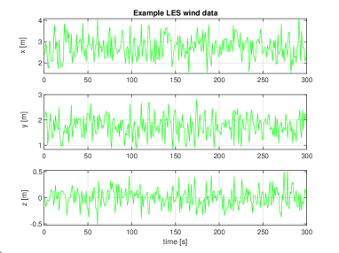
Figure 1: LES wind velocity in $x$, $y$ and $z$ direction. Wind in the $x$ direction has the highest mean and variance and the $z$ direction has the lowest mean and variance. This data is extracted at the position $(1,1,8)$ meters.

4.2 Tracking with LES Wind

We incorporate LES turbulence wind to test and validate the controller designs. For the drag coefficient $D$, we use Allison et al. (2020)

$$D=\min(1.1,(0.2+0.9\exp{(-0.6\lvert\lvert v_{w}-\dot{p}\rvert\rvert-2)}))I_{3}$$ (42)

where $I_{3}$ is the identity matrix. For simplicity, we consider $m=1$ kg. For trajectory tracking, the initial conditions are $x_{0}=[0,~{}0,~{}0,~{}1,~{}0,~{}0,~{}0,~{}0.001,~{}0,~{}0]^{T}$ and $u_{0}=[0,~{}0,~{}0,~{}10]^{T}$. Note that we start with at least one non-zero entries of velocity $v$ so that we do not get division by zero error from drag component of (4) during linearization. Since we are only dealing with trajectories at the altitude lower than $8$ m, we extracted $10$ minutes of LES data around our nominal trajectory points. The mean wind velocity of the extracted wind data is $\bar{v}_{w}=[2.72,~{}1.752,~{}-0.006]^{T}$ m/s.

We compare our results with a traditional LQR architecture using the same dynamics described in Section 2.2. We choose the cost such that the disturbance free trajectory matches the nominal trajectory closely. The quadratic cost for every simulation is fixed at $Q=diag([10,10,10,1,1,1,1,0.1,0.1,0.1])$ and $R=diag([1,5,5,0.1])$. We set the final cost is set at $Q_{f}=diag([20,20,20,0.1,0.1,0.1,0.1,0.1,0.1,0.1])$, for the finite horizon controller design.

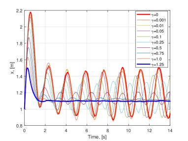
Figure 2: Change in trajectory in hover with increasing $\gamma$. Red indicates the LQR trajectory $(\gamma=0)$ and Blue indicates the MCV trajectory with $(\gamma=1.25)$. Increasing $\gamma$ reduces the variance.

To compare the effect of the tuning parameter $\gamma$, we simulate a hovering scenario at the position $(1,1,8)$ meters with multiple $\gamma$. We show the evolution of $p_{x}$ trajectory with varying $\gamma$ in Fig 2, where we observe that the maximum value $\gamma=1.25$ significantly reduces the variances in the trajectory. Figs 3 and 4 show that increase in $\gamma$ value results in decrease in the variance and the Root Mean Square (RMS) error. Only in the $z$ direction, there is minuscule increase in the RMS error, however the values are still significantly lower comparing to the smaller $\gamma$ values.

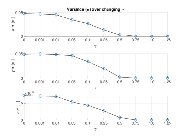
Figure 3: Change in trajectory variance in $x$, $y$, and $z$ directions with $\gamma$. As the $\gamma$ value increases, the variance decreases.

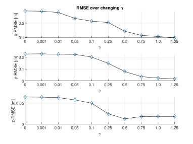
Figure 4: RMS error vs $\gamma$ illustrating the decrease in error with increasing $\gamma$.

We next employ the finite horizon MCV controller illustrated in Algorithm 2 for trajectory tracking problems. For the reference trajectories, we choose a straight line trajectory and a circular trajectory generated from minimum snap trajectories described in Mellinger and Kumar (2011).

Simulation results for the straight line reference trajectory are illustrated through Figs 5–7, where we use $\gamma=0.75$. The trajectories of the LQR and the MCV controllers along with the nominal trajectory are plotted in Fig 5, which demonstrate the effectiveness of MCV over LQR in reducing variance. We also conduct $50$ Monte Carlo simulations, where we incorporate different wind data and calculate the variance and the RMS error at each reference point. The trajectory with the MCV controller has smaller and smoother variance (see Fig 6) and RMS error (see Fig 7). A comparison of input signal $u$ is presented in Fig 8.

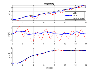
Figure 5: Comparison of straight line trajectory tracking with the LQR and the MCV controllers. Black is the nominal snap trajectory, blue corresponds to the MCV and red corresponds to the LQR trajectory. The deviation is smaller with the MCV controller.

Figure 6: Comparison of error variance calculated at each point over 50 Monte Carlo simulations between the MCV and the LQR controllers for the straight line trajectory tracking.

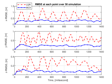
Figure 7: Comparison of RMSE calculated at each point over 50 Monte Carlo simulations between the MCV and the LQR controllers for the straight line trajectory tracking.

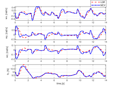
Figure 8: Comparison of input signals between the MCV and the LQR controllers for the straight line trajectory tracking. The MCV controller appears to have a faster response than the LQR controller.

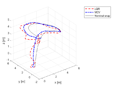
Figure 9: Comparison of circular trajectory tracking between the LQR and the MCV controllers (3D view).

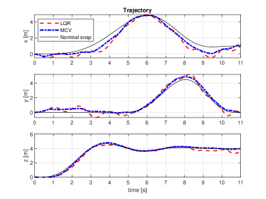
Figure 10: Comparison of circular trajectory tracking between the LQR and the MCV controllers for each direction.

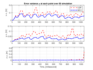
Figure 11: Comparison of error variance calculated at each point over 50 Monte Carlo simulations between the MCV and the LQR controllers for the circular trajectory tracking.

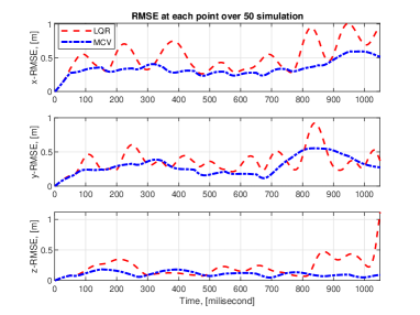
Figure 12: Comparison of the RMSE calculated at each point over 50 Monte Carlo simulations between the MCV and the LQR controllers for the circular trajectory tracking.

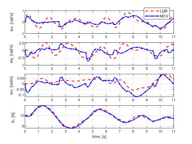
Figure 13: Comparison of input signals between the MCV and the LQR controllers for the circular trajectory tracking.

We also generate a minimum snap circular trajectory as the reference trajectory. The trajectory passes through $(1,0,4),~{}(4,0,4),~{}(4,3,4)$ and $(1,3,4)$ starting from $(0,0,0)$. For the MCV controller, we set $\gamma=0.50$. The 3D circular tracking is provided in Fig 9 and individual axis trajectory comparison in Fig 10. As expected, the MCV controller results in lower variance and RMS error as illustrated in Figs 11–12. Overall we notice:

• MCV reduces the variances as well as the RMS error of the trajectory. Although there still exists mean error, the variability is notably reduced.

• In the straight line trajectory, the error variance in the $x$ direction is lower than $0.08$ m with the MCV where with the LQR the variance rises up to $0.245$ m, which is more than $3$ times than the MCV. In the $y$ direction, the MCV reduces the variance as much as $7$ times than the LQR (refer to Fig 6).

• Although the circular trajectory exhibits higher variance than that of a straight line trajectory, the MCV controller still leads to tracking with a smaller variance than LQR (refer to Fig 10).

• From the input signal comparison in Fig 8 and Fig 13, we observe that in both cases the MCV controller responds earlier than the LQR controller. Also, the MCV controller input changes more as it reduces the noisy instances.

5 Future Work

We design a Minimum Cost Variance controller for quadrotor control in a wind field. Our simulation results demonstrate its effectiveness in reducing the tracking error and variance in a turbulent wind field. We aim to implement the controller in higher-fidelity quadrotor simulator platforms, preferably in the ROS-Gazebo environment and simulate with spatial-temporal wind data. We are also exploring design methodologies to accommodate the nonlinearity in the dynamics into the controller.

References

- Allison et al. (2020) Allison, S., Bai, H., and Jayaraman, B. (2020). Wind estimation using quadcopter motion: A machine learning approach. Aerospace Science and Technology, 98, 105699.
- Beare et al. (2006) Beare, R.J., Macvean, M.K., Holtslag, A.A., Cuxart, J., Esau, I., Golaz, J.C., Jimenez, M.A., Khairoutdinov, M., Kosovic, B., Lewellen, D., et al. (2006). An intercomparison of large-eddy simulations of the stable boundary layer. Boundary-Layer Meteorology, 118(2), 247–272.
- Bisheban and Lee (2018) Bisheban, M. and Lee, T. (2018). Geometric adaptive control for a quadrotor uav with wind disturbance rejection. In 2018 IEEE Conference on Decision and Control (CDC), 2816–2821. IEEE.
- Bryan and Fritsch (2002) Bryan, G.H. and Fritsch, J.M. (2002). A benchmark simulation for moist nonhydrostatic numerical models. Monthly Weather Review, 130(12), 2917–2928.
- Computational and Laboratory (2017) Computational and Laboratory, I.S. (2017). Cheyenne: Hpe/sgi ice xa system (university community computing).
- Davoudi et al. (2020) Davoudi, B., Taheri, E., Duraisamy, K., Jayaraman, B., and Kolmanovsky, I. (2020). Quad-rotor flight simulation in realistic atmospheric conditions. AIAA Journal, 58(5), 1992–2004.
- Deardorff (1980) Deardorff, J.W. (1980). Stratocumulus-capped mixed layers derived from a three-dimensional model. Boundary-Layer Meteorology, 18(4), 495–527.
- Ding and Wang (2018) Ding, L. and Wang, Z. (2018). A robust control for an aerial robot quadrotor under wind gusts. Journal of Robotics, 2018.
- Foehn and Scaramuzza (2018) Foehn, P. and Scaramuzza, D. (2018). Onboard state dependent lqr for agile quadrotors. In 2018 IEEE International Conference on Robotics and Automation (ICRA), 6566–6572. IEEE.
- Gill and D’Andrea (2017) Gill, R. and D’Andrea, R. (2017). Propeller thrust and drag in forward flight. In 2017 IEEE Conference on Control Technology and Applications (CCTA), 73–79. IEEE.
- Hamadi et al. (2019) Hamadi, H., Lussier, B., Fantoni, I., Francis, C., and Shraim, H. (2019). Observer-based super twisting controller robust to wind perturbation for multirotor uav. In 2019 International Conference on Unmanned Aircraft Systems (ICUAS), 397–405. IEEE.
- Jiang and Shu (1996) Jiang, G.S. and Shu, C.W. (1996). Efficient implementation of weighted eno schemes. Journal of computational physics, 126(1), 202–228.
- Mellinger and Kumar (2011) Mellinger, D. and Kumar, V. (2011). Minimum snap trajectory generation and control for quadrotors. In 2011 IEEE International Conference on Robotics and Automation, 2520–2525. 10.1109/ICRA.2011.5980409.
- Sain (1965) Sain, M.K. (1965). On minimal-variance control of linear systems with quadratic loss. Technical report, ILLINOIS UNIV URBANA COORDINATED SCIENCE LAB.
- Sain et al. (1995) Sain, M.K., Won, C.H., and Spencer, B. (1995). Cumulants in risk-sensitive control: The full-state-feedback cost variance case. In Proceedings of 1995 34th IEEE Conference on Decision and Control, volume 2, 1036–1041. IEEE.
- Sierra and Santos (2019) Sierra, J.E. and Santos, M. (2019). Wind and payload disturbance rejection control based on adaptive neural estimators: application on quadrotors. Complexity, 2019.
- Smagorinsky (1963) Smagorinsky, J. (1963). General circulation experiments with the primitive equations: I. the basic experiment. Monthly weather review, 91(3), 99–164.
- Tran et al. (2015) Tran, N.K., Bulka, E., and Nahon, M. (2015). Quadrotor control in a wind field. In 2015 International Conference on Unmanned Aircraft Systems (ICUAS), 320–328. IEEE.
- Tran et al. (2021) Tran, V.P., Santoso, F., and Garratt, M.A. (2021). Adaptive trajectory tracking for quadrotor systems in unknown wind environments using particle swarm optimization-based strictly negative imaginary controllers. IEEE Transactions on Aerospace and Electronic Systems.
- Von Karman (1948) Von Karman, T. (1948). Progress in the statistical theory of turbulence. Proceedings of the National Academy of Sciences of the United States of America, 34(11), 530.
- Wang et al. (2016) Wang, C., Song, B., Huang, P., and Tang, C. (2016). Trajectory tracking control for quadrotor robot subject to payload variation and wind gust disturbance. Journal of Intelligent & Robotic Systems, 83(2), 315–333.
- Won et al. (2003) Won, C.H., Sain, M.K., and Liberty, S.R. (2003). Infinite-time minimal cost variance control and coupled algebraic riccati equations. In Proceedings of the 2003 American Control Conference, 2003., volume 6, 5155–5160. IEEE.
- Yang et al. (2017) Yang, H., Cheng, L., Xia, Y., and Yuan, Y. (2017). Active disturbance rejection attitude control for a dual closed-loop quadrotor under gust wind. IEEE Transactions on control systems technology, 26(4), 1400–1405.
- Zhang et al. (2016) Zhang, C., Zhou, X., Zhao, H., Dai, A., and Zhou, H. (2016). Three-dimensional fuzzy control of mini quadrotor uav trajectory tracking under impact of wind disturbance. In 2016 International Conference on Advanced Mechatronic Systems (ICAMechS), 372–377. IEEE.