The Atacama Cosmology Telescope: A search for Planet 9

Abstract

We use Atacama Cosmology Telescope (ACT) observations at 98 GHz (2015–2019), 150 GHz (2013–2019) and 229 GHz (2017–2019) to perform a blind shift-and-stack search for Planet 9. The search explores distances from 300 AU to 2000 AU and velocities up to 6.3 arcmin per year, depending on the distance ($r$). For a 5 Earth-mass Planet 9 the detection limit varies from 325 AU to 625 AU, depending on the sky location. For a 10 Earth-mass planet the corresponding range is 425 AU to 775 AU. The search covers the whole 18 000 square degrees of the ACT survey. No significant detections are found, which is used to place limits on the mm-wave flux density of Planet 9 over much of its orbit. Overall we eliminate roughly 17% and 9% of the parameter space for a 5 and 10 Earth-mass Planet 9 respectively. We also provide a list of the 10 strongest candidates from the search for possible follow-up. More generally, we exclude (at 95% confidence) the presence of an unknown Solar system object within our survey area brighter than 4–12 mJy (depending on position) at 150 GHz with current distance $300\text{ AU}<r<600\text{ AU}$ and heliocentric angular velocity $1.5^{\prime}/\text{yr}<v\cdot\frac{500\text{ AU}}{r}<2.3^{\prime}\text{yr}$, corresponding to low-to-moderate eccentricities. These limits worsen gradually beyond 600 AU, reaching 5–15 mJy by 1500 AU.

1 Introduction

The existence of “Planet 9”, a large (mass $M\sim 5-10$ $M_{\earth}$) and very distant (semi-major axis $a\sim 400-800$ AU) new planet in the solar system, has recently been proposed as an explanation for the observed clustering of orbits of the highest-perihelion objects in the detached Kuiper belt (Batygin & Brown, 2016; Batygin et al., 2019) (hereafter B16 and B19). While the reality of this clustering is unclear because of the presence of large observational biases (Shankman et al., 2017; Bernardinelli et al., 2020; Napier et al., 2021; Brown, 2021), the hypothesis has still gathered considerable interest.

Most new solar system objects are discovered in optical surveys via their reflected sunlight. At these wavelengths, Planet 9 would appear as a magnitude 19–24 object (depending on the size and distance and assuming an albedo between 0.4 and 1) (page 61 B19): quite faint due to the $1/r^{4}$ dependence of reflected sunlight, but still detectable by optical surveys like the Dark Energy Survey (DES), the Hyper-Suprime Cam survey (HSC) or the Legacy Survey of Space and Time (LSST).

The steep fall-off of flux density with distance can be circumvented by observing at longer wavelengths, where thermal emission dominates. The heat budget of large objects far from the Sun is dominated by their gravitational contraction and residual heat of formation, resulting in a temperature that is approximately independent of their distance from the Sun. This leads to a much gentler $1/r^{2}$ dependence. For sufficiently large distances this can partially compensate for, or even overcome, the resolution advantage enjoyed by optical surveys compared to those at mm or sub-mm wavelengths. Indeed, the best current limits on the existence of Saturn- or Jupiter-size trans-Neptunian objects (TNOs) is the Wide-Infrared Survey Explorer (WISE), which observes in the 2.8–26 $\micro$m (11–110 THz) range. WISE has excluded the existence of a Saturn-size planet out to 28 000 AU, and a Jupiter-size one out to 82 000 AU (Luhman, 2013). Sadly, these limits degrade very quickly with mass, partially because of a decrease in surface area, but more importantly because lower-mass planets cool down more quickly. For sufficiently low masses, the majority of the thermal emission would fall outside the WISE frequency range, and this is expected to be the case for typical atmospheric models (see section 2). However, emission predictions in the 3-5 $\micro$m window are extremely model dependent, varying by four orders of magnitude. The brightest of these could be detectable by WISE. Meisner et al. (2018) report a non-detection of Planet 9 in WISE’s 3.6 $\micro$m W1 band, limiting its W1 magnitude to $>16.7$ (flux density $<65\text{ }\micro$Jy) at 90% confidence. For the most optimistic atmospheric models, this excludes a $10M_{\earth}$ Planet 9 up to 900 AU, but for more typical cases WISE would not be sensitive to Planet 9’s thermal radiation, motivating a search at lower frequencies.

Soon after Planet 9 was first proposed, Cowan et al. (2016) (and later Baxter et al. (2018)) suggested a search using Cosmic Microwave Background (CMB) telescopes operating in the 1–3 mm range. The only current CMB survey telescopes with high enough resolution to have any hope of detecting a faint, unresolved object like Planet 9 are the South Pole Telescope (SPT) (Carlstrom et al., 2011) and the Atacama Cosmology Telesope (ACT) (Fowler et al., 2007; Thornton et al., 2016), and of these only ACT covers the low ecliptic latitudes where Planet 9 might lurk.

ACT is a 6-m mm-wave telescope located at 5190 m altitude on Cerro Toco in the northern Chilean Andes. ACT began observations in 2008, and has been upgraded several times to add polarization support and increase its sensitivity and frequency coverage. ACT is currently surveying 18 000 square degrees of the sky in five broad bands roughly centered on 27 GHz, 39 GHz, 98 GHz, 150 GHz and 229 GHz, though the first two were added too recently to be available for this analysis. We label these bands f030, f040, f090, f150 and f220 respectively.

The primary goal of the survey is to map the CMB, but the telescope’s relatively high angular resolution of 2.05/1.40/0.98 arcminutes full-width-half-max (FHWM) in the f090/f150/f220 bands respectively makes it capable of a large set of other science goals, including searches for galaxy clusters, active galactic nuclei and transients. We here report on a search for Planet 9 using 7 years of ACT data collected from 2013 to 2019.

2 Planet 9 in the ACT bands

Fortney et al. (2016) (henceforth F16) investigated the radius, temperature and luminosity of Planet 9, and found that the Sun had a minimal impact on its heat budget, and hence its physical properties do not depend on the planet’s distance from the Sun. They do, however, depend considerably on both its mass and internal composition, for which F16 build several models.

Their nominal scenario has a H/He envelope making up 10% of the planet’s mass, with the remainder being mostly a 2:1 mix of ice and rock. For this composition they find that the most favored $5M_{\earth}$ scenario of B19 results in a radius of $2.94R_{\earth}$, a temperature of 42.2 K and a featureless blackbody spectrum below 8 THz. For a fiducial distance of 500 AU, this results in a flux density of 2.3 mJy, 5.3 mJy and 11 mJy in the three ACT bandpasses f090, f150 and f220. For the $10M_{\earth}$ scenario, which is near the upper end of the possible mass range, the corresponding numbers are $R=3.46R_{\earth}$, $T=48.3\text{K}$ and a flux density of 3.7/8.5/18 mJy at f090/f150/f220. These numbers vary by 10–50% depending on the composition – see Table 1. Depending on Planet 9’s exact orbit, its current distance could vary from about 300 AU to 1200 AU, but due to the radius and temperature being independent of the distance from the Sun, this simply rescales the flux densities as $1/r^{2}$.

The expected distance to Planet 9 is correlated with its mass, since a more massive planet has to be further away to avoid having too large of an effect on the orbits of other trans-Neptunian objects. A $5M_{\earth}$ Planet 9 would have an expected semi-major axis $a\sim 500$ AU and an eccentricity of $0.1\lessapprox e\lessapprox 0.3$, while at $10M_{\earth}$ the best-fit semi-major axis and eccentricity are $a\sim 700$ AU and $0.3\lessapprox e\lessapprox 0.5$ (fig. 15 B19). At frequencies $<2.5\text{ THz}$, this increased distance mostly cancels the increased luminosity of a more massive planet, making ACT’s prospect for detecting an object like Planet 9 only moderately sensitive to its mass. The planet’s inclination is predicted to be moderate, $i<30^{\circ}$, with $i\approx 20^{\circ}$ preferred.

To see if ACT has any chance of detecting this signal, let us compare it to ACT’s sensitivity to stationary point sources. This varies by position in the map but the 10–90% quantile range is about 1–2 mJy at f090 and f150, and 4–8 mJy at f220. Hence, if Planet 9 were stationary at 500 AU, we could expect to detect it at $2.3-11\sigma$ for the $5M_{\earth}$ case when combining the three ACT bands. This is not high enough to guarantee a discovery, especially considering that Planet 9 could be at a larger distance than 500 AU, but it’s high enough that a search is worthwhile.

Figure 1 compares the brightest/medium/faintest expected Planet 9 spectra (as inferred from the range of possible orbits from B19 and of physical properties from F16) to the sensitivity of ACT and other current and future wide-area surveys. Despite WISE’s impressive bounds on Saturn- and Jupiter-size TNOs, it is not very sensitive to smaller, and therefore colder, objects like Planet 9. The most sensitive current data set that covers most/all of Planet 9’s orbit is therefore Pan-STARRS. At its full depth of about magnitude 23, Pan-STARRS has a flux density limit of roughly 2 $\micro$Jy, but this degrades to around 20 $\micro$Jy (mag. $\approx 21$) if the search is limited to the depth of the Pan-STARRS transient search (Pan-STARRS, 2015, B19). Both WISE and Pan-STARRS have reduced sensitivity near the galactic plane because of confusion. For the medium brightness case, ACT’s typical depth could expect a borderline detection, similar to the Pan-STARRS transient search and a bit better than WISE.

Mass	Radius	Temperature	Band	Flux @ 500 AU	ACT Depth	FWHM	Freq.
$\text{M}_{e}$	$\text{R}_{e}$	K	-	mJy	mJy	arcmin	GHz
5	4.12/2.94/2.71	36.7/42.2/38.9	f090	3.9/2.3/1.8	1.0–2.1	2.05	98
			f150	8.9/5.3/4.1	1.0–2.2	1.40	150
			f220	18/11/8.5	4.1–8.4	0.98	229
10	5.09/3.46/3.16	40.3/48.3/45.1	f090	6.6/3.7/2.9	1.0–2.1	2.05	98
			f150	15/8.5/6.6	1.0–2.2	1.40	150
			f220	31/18/14	4.1–8.4	0.98	229

Table 1: Potential radii and temperatures for a $5M_{\earth}$ and $10M_{\earth}$ Planet 9 from F16. The three slash-separated entries correspond to three planet types described in their Table 1. The central one is the nominal case with a 2:1 ice:rock core surrounded by an H/He envelope. The leftmost entries are for a case with a larger H/He envelope and the rightmost entries are for the ice-poor case, for which the core is 1:2 ice:rock by mass. The corresponding flux density in the three ACT frequency bands for these cases is given in the flux density column, and compared to the ACT point source sensitivity, which is about 1–2 mJy as seen in the sixth column. The first/last number in the range of ACT depth is the 10%/90% quantile over the 18,000 square degrees that ACT covers. The maps are deep enough compared to the expected Planet 9 flux density that a search is worthwhile. Also shown are the ACT beam size and central frequency in each band.

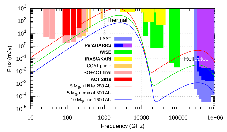
Figure 1: The potential Planet 9 spectra compared to the $5\sigma$ detection limit of current and upcoming wide-area surveys. Red curve: High-brightness scenario: a $5M_{\earth}$ Planet 9 with a heavy H/He envelope at a perihelion of 288 AU. Green curve: A more moderate scenario with a light H/He envelope and a 2:1 ice:rock ratio at 500 AU, still with $5M_{\earth}$. Blue curve: Low-brightness scenario: A $10M_{\earth}$ Planet 9 with a light H/He envelope and a 1:4 ice:rock ratio at an aphelion of 1160 AU. All scenarios assume unit emissivity black-body spectra, but differ in the planet radius and release and transport of internal gravitational energy; see F16 Table 1. ACT 2019 is the data-set used in this paper, while SO+ACT final is the expected combined Simons Observatory (SO Collaboration, 2019) + ACT data after both surveys finish. The others are CCAT-prime (Choi et al., 2020), IRAS (W.G., 1986), AKARI (Ishihara et al., 2010; Yamamura et al., 2010), WISE (AllWISE, 2013; Schlafly et al., 2019), Pan-STARRS (Chambers et al., 2016) and LSST (Ivezić et al., 2019). Future surveys are shown with a thinner font and less intense color in the legend. For Pan-STARRS both the full depth (blue) and the transient search depth (purple) (Pan-STARRS, 2015) are shown. The double blackbody approximation used here may be inaccurate in the range 8-400 THz because of atmospheric features (Fig. 1 F16). The sensitivities shown are typical values for each survey, and do not attempt to compensate for the surveys’ different sky coverage. Depth variations inside each survey and the effect of the large parameter space of a blind search for a moving object are ignored.

3 The ACT data sets

The data sets used in this analysis are identical to those used in Naess et al. (2020a), except for the inclusion of one more season of data (2019), and the exclusion of the Planck and ACT MBAC data sets because of their low resolution and low sky coverage respectively. This represents 7 years and 140 TB of data, of which 81% was collected since the AdvACT camera (Ho et al., 2017; Choi et al., 2018) became operational in 2017 (i.e., after ACT Data Release 4). See Appendix D for details.

4 Search methodology

4.1 Blink comparison won’t work

The most common way to discover solar system objects is to look for objects that have moved between two different exposures of the same patch of sky. This method is fast, but is limited by the depth of each image, since the object needs to be independently detected in both. This depth can be improved with longer exposures, but this is limited by the angular velocity of the object itself. Integrating longer than the time it takes the object to move by the size of the beam will just smear it out without any further gains in S/N. This is the regime ACT is in for Planet 9.

For ACT sky coverage and sensitivity, it would take 3–4 years of observations just to have a chance of detecting a Planet 9-like object that was not moving in the sky. By Kepler’s laws, a planet with semi-major axis $a$, eccentricity $e$ and current solar distance $r$ will have a Sun-centered angular speed of

$$v =1.932^{\prime}/\text{yr}\cdot\sqrt{\frac{a}{\text{500 AU}}}\left(\frac{r}{\text{500 AU}}\right)^{-2}\sqrt{1-e^{2}}.$$ (1)

At the same time, the Earth’s orbit sweeps out a yearly parallax ellipse with a semi-major axis of

$$\theta_{\pi} =\frac{\text{AU}}{r}=6.875^{\prime}\cdot\frac{500\text{AU}}{r}$$ (2)

corresponding to a maximum angular speed of

$$v_{\pi} =\frac{2\pi\theta_{\pi}}{\textrm{yr}}=43.20^{\prime}/\text{yr}\cdot\frac{500\text{AU}}{r}.$$ (3)

For comparison, ACT has an angular resolution of 2.05/1.40/0.98’ FWHM at f090/f150/f220 respectively. To avoid excessive smearing we need $(v_{\pi}+v)\Delta t\approx v_{\pi}\Delta t\ll\text{FWHM}$. For the smallest beam (f220) and a closest possible distance of $r_{\textrm{min}}=300$ AU, this gives us $\Delta t\ll 5\text{ days}$. With 5 days of integration time and the current ACT survey strategy the expected Planet 9 S/N would be $\sim 1$, more than 5 times too low for a detection, or more than 25 times too low in terms of observing time!

4.2 Shift and stack

The smearing could be eliminated if one knew the orbit of the object one was looking for, since that would allow one to shift each exposure to track the object as it moves across the sky. In practice, while the Planet 9 hypothesis makes some predictions about its orbit, they are far too vague to allow for simple tracking like this. However, with enough computational resources it is possible to loop through every reasonable orbit, make a shifted stack of individual short exposures using that orbit, and then look for objects in the resulting image. This is the shift-and-stack algorithm, and has been used to successfully detect objects below the single-exposure sensitivity limit (Gladman et al., 1998; Holman et al., 2018),

Planet 9’s orbit is characterized by its 6 orbital elements: semi-major axis $a$, eccentricity $e$, inclination $i$, longitude of ascending node $\Omega$, argument of periapsis $\omega$ and true anomaly $\nu$. However, because of its large distance and corresponding slow motion, it is sufficient for us to consider its motion to be drifting linearly on the sky, modulated by parallax. This gives us the following 5 free parameters:

1. The heliocentric right ascension ($\alpha$) and declination ($\delta$) of the planet at a reference time $t_{0}$.

2. The horizontal and vertical components of the heliocentric angular velocity $\vec{v}=[v_{x},v_{y}]$. We define these in the local tangent plane, such that $\alpha_{\text{obs}}=\alpha+v_{x}(t-t_{0})/\cos\delta_{0}$ and $\delta_{\text{obs}}=\delta+v_{y}(t-t_{0})$.

3. The planet’s current distance from the Sun, $r$, which we treat as constant in time.

With these, the shift-and-stack algorithm takes the following general form:

1. Split the data into chunks with duration $\Delta t$, and make a sky map of each.

2. For each reasonable value of $r,v_{x},v_{y}$, use these with the time $t$ of each map to shift them according to their constant heliocentric angular velocity and parallactic motion, and stack them to produce a combined map.

3. Use a filter matched to the noise and signal properties to look for point sources in each combined map.

We will go through the details of this process in the following sections.

4.3 Mapping and the matched filter

4.3.1 The sky maps

ACT observes the sky by sweeping backwards and forwards in azimuth while the sky drifts past. As it does so, the temperature registered by the detectors is read out hundreds of times per second, forming a vector of time-ordered-data $d$. We model $d$ as

$$d =Pm+n,$$ (4)

where $m$ is the (beam-convolved, pixelated) sky in $\micro$K CMB temperature units, $P$ is a response matrix that encodes the telescope’s pointing as a function of time, and $n$ is instrumental and atmospheric noise which we model as Gaussian covariance $N$. The maximum-likelihood estimate for $m$ given $d$ is

$$\hat{m} =(P^{T}N^{-1}P)^{-1}P^{T}N^{-1}d$$

$$M =(P^{T}N^{-1}P)^{-1}$$ (5)

Here $M$ is the noise covariance matrix of the estimator $\hat{m}$.

4.3.2 The matched filter

To look for point sources in $\hat{m}$ we start by assuming that all sources are far enough apart that they can be considered in isolation. Our data model for a map containing a single point source in some pixel $p$ is then

$$\hat{m} =RQs_{p}+u$$ (6)

where $s_{p}$ is the point source flux density in pixel $p$ in mJy at a reference frequency $\nu_{0}=150\text{ GHz}$ and $Q_{i}=\delta_{ip}$ is a vector that’s unity at the source location in pixel $p$ and zero elsewhere. It takes us from just a single flux density value to a map with that value in a single pixel.

$R=Bg(\nu_{0},\nu)f(\nu)A_{p}$ is a response matrix that takes us from that map to beam-convolved $\micro$K at the observed frequency. Here $B$ is the instrument beam normalized to have a pixel-space integral of one, $g(\nu_{0},\nu)$ is the conversion factor from flux density at the reference frequency $\nu_{0}$ to the observed frequency $\nu$, $f(\nu)$ is the conversion from flux density in mJy to beam-convolved peak height in $\micro$K, and $A_{p}$ is pixel area in steradians. Since we expect Planet 9 to be a blackbody with temperature $T\approx 40$ K, we have $g(\nu_{0},\nu)=b(\nu,T)/b(\nu_{0},T)$, where

$$b(\nu,T) =\frac{2h\nu^{3}}{c^{2}}\frac{1}{\exp\left(\frac{h\nu}{k_{B}T}\right)-1}$$ (7)

is the Planck law for surface brightness $b$; and

$$f(\nu) =\left(\frac{2x^{4}k_{B}^{3}T_{\text{CMB}}^{2}}{h^{2}c^{2}}\frac{1}{4\sinh(x/2)^{2}}10^{23}A_{b}\right)^{-1}$$ (8)

$$x =\frac{h\nu}{k_{B}T_{\text{CMB}}}.$$

Finally, $u$ is the noise in $\hat{m}$ and has a covariance matrix $U$. For the purposes of point source detection, $u$ consists of everything in $\hat{m}$ that isn’t the point source, which includes both the instrumental and atmospheric noise described by the $M$ covariance matrix from before, but also the CMB, Cosmic Infrared Background (CIB), galactic dust, etc.

Given this model for $\hat{m}$, the maximum-likelihood estimate for the point source flux density at the reference frequency is

$$\hat{s}_{p} =\rho_{p}/\kappa_{p}, \rho_{p} =Q^{T}R^{T}U^{-1}\hat{m}$$

$$\sigma_{\hat{s}_{p}} =1/\sqrt{\kappa_{p}}, \kappa_{p} =Q^{T}R^{T}U^{-1}RQ$$ (9)

Here $\sigma_{\hat{s}_{p}}$ is the standard deviation of $\hat{s}_{p}$, $\kappa_{p}$ corresponding inverse variance, and $\rho_{p}$ is the inverse variance weighted flux density.

So far we have only estimated the point source flux density in some pixel $p$. But since we don’t a priori know where on the sky the planet could be, we need to estimate the flux density in every pixel, resulting in the flux density sky map $\hat{s}$ and corresponding uncertainty $\sigma_{\hat{s}}$ given by:

$$\hat{s} =\rho/\kappa, \rho =R^{T}U^{-1}\hat{m}$$

$$\sigma_{\hat{s}} =1/\sqrt{\kappa}, \kappa =\text{diag}(R^{T}U^{-1}R)$$ (10)

where the division is done pixel by pixel. The corresponding S/N is

$$S/N =\vec{s}/\sigma_{\vec{s}}=\rho/\sqrt{\kappa}=\frac{R^{T}U^{-1}\hat{m}}{\sqrt{\text{diag}(R^{T}U^{-1}R)}}$$ (11)

which we recognize as the matched filter for $\hat{m}$. This S/N map is what one would usually use for object detection, e.g. by identifying peaks with $S/N>5$. As we shall see in Section 4.7 the shift and stack parameter search complicates this, but the general idea stays the same.

4.3.3 Stacking

If we have multiple estimates $\{\vec{s}_{i}\}$ built from independent chunks of data, such as the few-day chunks we will use in the shift-and-stack algorithm, these combine straightforwardly:

$$\rho_{\text{tot}} =\sum_{i}\rho_{i}, \kappa_{\text{tot}} =\sum_{i}\kappa_{i}$$

$$\vec{s}_{\text{tot}} =\rho_{\text{tot}}/\kappa_{\text{tot}}, \sigma_{\vec{s}_{\text{tot}}} =1/\sqrt{\kappa_{\text{tot}}}$$ (12)

Sadly, the presence of the same CMB, CIB etc. in each chunk of data breaks the assumption of independence that this expression builds on. It would be possible to build a more complicated expression that takes this into account, but given the computationally expensive parameter search we perform we need the stacking operation to be as fast and simple as possible. Thankfully we can eliminate these correlated components by simply subtracting the time-averaged mean of the sky from each chunk of data.

4.3.4 Mean sky subtraction

We can avoid the complications of the CMB, CIB etc. acting as correlated noise common to the data chunks by subtracting a high-S/N estimate of the mean sky from each chunk of data before mapping it. This eliminates any static part of the sky such as the CMB, CIB, galactic emission, etc. (including any we don’t know about), and leaves only time-dependent signals such as the planet we’re looking for, as well as variable point sources (which can be masked) and transients (which are rare enough that we can ignore them). The cost is a small increase in the noise if the mean sky model isn’t noise-free, and a partial subtraction of the signal itself that must be estimated and corrected for. For this search we use the ACT+Planck combined maps described in Naess et al. (2020a), but extended to include the 2019 season of data.

Aside from letting us stack using equation 12, mean sky subtraction has the effect of removing all but the instrumental and atmospheric noise from the individual sky maps, and hence the matched filter noise covariance matrix $U$ reduces to $M$. Inserting this into equation 10 we get:

$$\rho =R^{T}\overbrace{P^{T}N^{-1}d}^{\text{rhs}}$$ (13)

The part labeled “rhs” is a map that is much cheaper to compute than $\hat{m}$ because it avoids the expensive inversion $(P^{T}N^{-1}P)^{-1}=M$ which must usually be done using iterative methods like Conjugate Gradients. That leaves us with $\kappa$ which we approximate as

$$\kappa_{i} =R_{ji}M^{-1}_{jk}R_{ki}\approx\alpha R_{ji}^{2}w_{j}$$ (14)

where the map $w$ is an approximation pixel-diagonal of $M^{-1}$ built assuming white (uncorrelated) noise and $\alpha$ is a factor that compensates for the mean error we make by replacing $M^{-1}$ with $\vec{w}$. We determine $\alpha$ by evaluating a few pixels of the exact $\kappa$.

4.3.5 Ad-hoc filter

Due to the time-domain noise model underestimating the amount of correlated noise in the data, we applied an extra ad-hoc filter to the maps. This is described in Appendix C, but has the effect of suppressing noise for scales $\gtrsim 0.1^{\circ}$.

4.3.6 Point source handling

During map-making, any samples that were within 0.8 degrees of Venus, Mars, Jupiter, Saturn, Uranus or Neptune were cut to avoid both the planets themselves and 0.1–1%-level contamination through the near sidelobes. In addition, any sample within 3 arcminutes of the bright asteroids Vesta, Pallas, Ceres, Iris, Eros, Hebe, Juno, Melpomene, Eunomia, Flora, Bamberga, Ganymed, Metis, Nausikaa and Malasslia were cut.

To avoid false detections from variable point sources (e.g. blazars) we also cut point sources with a peak amplitude of at least 500 $\micro$K out to the radius where the beam has damped them to 10 $\micro$K. For daytime data, the peak amplitude threshold was reduced to 150 $\micro$K and the cut area was broadened by $\pm 1^{\prime}$ in azimuth and $-1^{\prime}$ to $4^{\prime}$ in elevation to account for the harder-to-model daytime beam and pointing. 500 $\micro$K corresponds to about 49/37/23 mJy in the f090/f150/f220 bands, and with this 2770/3054/1640 point sources were cut in the night and 9252/7886/1713 in the day. Point sources fainter than this (but still with $S/N>10$), of which there were 8868/5246/73 for the night-time and 2382/413/0 for daytime were individually fit and subtracted from the time-ordered data.

4.3.7 Dust masking

In theory all galactic dust should be canceled by the mean sky subtraction, since this represents length scales too large to evolve over the course of our observations. However, in practice small time-variable errors in our detector calibration can make the dust appear to fluctuate slightly in brightness. For sufficiently bright regions of dust these fluctuations become big enough to induce a large number of false positives in the search. Ideally we would use the dust signal itself to calibrate the detectors in these regions, but for now we simply mask them.

We built a dust mask by high-pass filtering the Planck PR2 545 GHz map with the Butterworth filter $\beta(\ell,1500,-5)$ (see Appendix C), selecting the 7% brightest pixels of the absolute value of the result, and growing the result by smoothing it with a Gaussian beam with $\sigma=7.2$ arcmin and masking areas with value $>0.5$. This mask was applied to each $\rho,\kappa$ map. We found that the edges of the mask introduce some artifacts during the shift-and-stack search, so we additionally applied a 20 arcmin larger mask before the final object detection step.

4.4 Search space

	300, 375, 500, 750 and 1500 AU	321, 409, 563, 900 and 2000 AU	346, 450, 643 and 1125 AU
$v_{y}$ (${}^{\prime}/\text{yr}$)
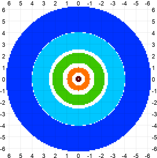
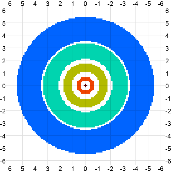
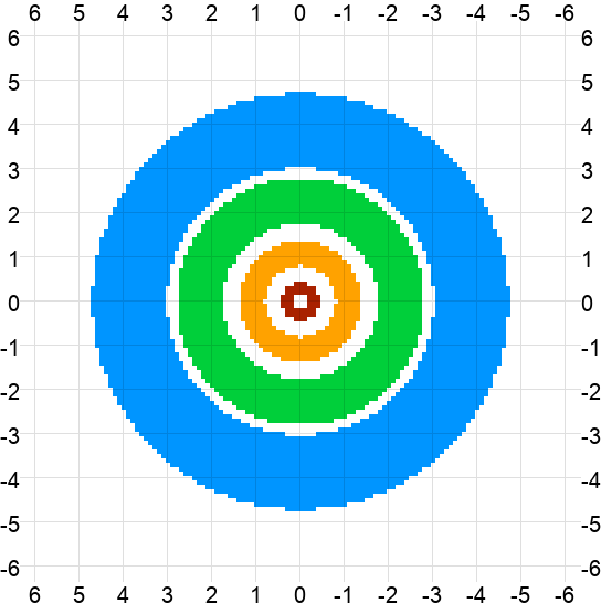
	$v_{x}$ (${}^{\prime}/\text{yr}$)	$v_{x}$ (${}^{\prime}/\text{yr}$)	$v_{x}$ (${}^{\prime}/\text{yr}$)

Figure 2: Illustration of the $r,v_{x},v_{y}$ search space used in the Planet 9 search. The horizontal and vertical axis shows $v_{x}$ and $v_{y}$ respectively, the components of the heliocentric angular velocity, in units of ^′/yr (arcmin per year). Each colored region corresponds to the velocities that were explored for a given solar distance $r$. From blue to red these are 300, 321, 346, 375, 409, 450, 500, 563, 643, 750, 900, 1125, 1500 and 2000 AU. The regions are spread over three sub-figures to avoid overlaps. The velocity grid used in the search had a 0.1^′/yr resolution, resulting in a total parameter volume of 25 837 cells.

$M$	$a$ (AU)		$e$		$q$ (AU)		$Q$ (AU)		$v_{\text{ref}}$ (′/yr)
5	350 -	450	0.10 -	0.20	280 -	405	385 -	540	1.58 -	1.82
5	450 -	550	0.20 -	0.30	315 -	440	540 -	715	1.75 -	1.99
10	650 -	750	0.30 -	0.40	390 -	525	845 -	1050	2.02 -	2.26
10	750 -	850	0.40 -	0.50	375 -	510	1050 -	1275	2.05 -	2.31

Table 2: Prior parameter ranges from Figure 15 of B19. This is based on the best-fit parameter points for the $5M_{\earth}$ and $10M_{\earth}$ scenarios, to which uncertainty ranges of $a\pm 50$ AU and $e\pm 0.05$ were added based on the resolution of the grid they used in their investigation. The planet mass, M, is given in Earth masses, e is the eccentricity, q is the perihelion distance and Q is the aphelion distance, both in AU. $v_{\text{ref}}$ is the planet’s hypothetical speed at a reference location of $r_{\text{ref}}=500$ AU. The planet’s actual speed will be $v=v_{\text{ref}}\frac{r_{\text{ref}}^{2}}{r^{2}}$.

The distance to and velocity of Planet 9 are relatively poorly determined, but we can infer rough limits on the acceptable fit from Figure 15 of B19, as shown in Table 2. We see that Planet 9’s current distance is limited to $300\text{AU}\lesssim r\lesssim 1300\text{AU}$. Equation 1 for the heliocentric angular velocity of the planet can be re-expressed as

$$v =v_{\text{ref}}\Big{(}\frac{r}{500\text{AU}}\Big{)}^{-2}$$ (15)

$$v_{\text{ref}} =1.93^{\prime}/\text{yr}\cdot\sqrt{a(1-e^{2})/(500\text{ AU})}$$ (16)

and from Table 2 we see that $v_{\text{ref}}$ is in the range 1.6 to 2.3 ^′/yr for all the acceptable fits. This means that only a hollow cone in our $r,v_{x},v_{y}$ parameter space needs to be explored.

While in theory there is a continuum of possible parameter values inside this cone, in practice the limited angular resolution of the telescope means that very similar parameters are indistinguishable. From equation 2 we see that getting the distance wrong by $\delta r$ results in a parallax ellipse that’s bigger by

$$\delta\theta_{r} \approx-0.14^{\prime}\cdot\frac{\delta r}{10\text{AU}}\Big{(}\frac{500\text{AU}}{r}\Big{)}^{2}.$$ (17)

Thus shift-stacking with the wrong distance leaves a residual ellipse with a radius of $|\delta\theta_{r}|$. If we step through distances in steps of $\Delta r$, then $\delta r$ will take on values in the range $[-\frac{\Delta r}{2},\frac{\Delta r}{2}]$. Using equations 17 and A4 from Appendix A, we see that on average, this increases the beam FWHM in quadrature by:

$$\Delta\text{FWHM}_{\text{r}} =0.093^{\prime}\cdot\frac{\Delta r}{10\text{AU}}\Big{(}\frac{500\text{AU}}{r}\Big{)}^{2}.$$ (18)

Similarly, getting the speed wrong by $\delta v$ will over a time $T=t-t_{0}$ accumulate to a position error of

$$\delta\theta_{v} =0.3^{\prime}\cdot\frac{\delta v}{0.1^{\prime}\text{/yr}}\frac{T}{3\text{yr}}.$$ (19)

For a velocity step of $\Delta v$ we get, using eq. A6,

$$\Delta\text{FWHM}_{v} =0.29^{\prime}\cdot\frac{\Delta v}{0.1^{\prime}\text{/yr}}\frac{T}{3\text{yr}}$$ (20)

where we have included a factor $\sqrt{2}$ in the numerical factor to take into account the smearing in both the $x$ and $y$ directions. The factor $T$ depends on when in the ACT observing campaign each observation was taken, but will at most be three years if we choose $t_{0}$ to be the mid-point of ACT observations. The integration time $\Delta t$ also results in smearing,

$$\Delta\text{FWHM}_{t} =0.080^{\prime}\cdot\frac{500\text{AU}}{r}\frac{\Delta t}{\text{day}}$$ (21)

as does the pixel window

$$\Delta\text{FWHM}_{\text{pix}} =0.68^{\prime}\cdot\frac{\text{res}}{1^{\prime}}$$ (22)

where res is the pixel side length. Together these effects make up our smearing budget, and each must be chosen small enough that their combined effect does not overly degrade the S/N. We choose

• $\Delta v=0.1^{\prime}/\text{yr }\Rightarrow\Delta\text{FWHM}_{v}=0.29^{\prime}$ for $T=3\text{ yr}$.

• $\Delta t=3\text{ days }\Rightarrow\Delta\text{FWHM}_{t}=0.40^{\prime}$ for $r=300\text{AU}$, which is the closest distance we will consider.

• $\Delta r=33\text{AU}\cdot\left(\frac{500\text{AU}}{r}\right)\Rightarrow\Delta\text{FWHM}_{r}=0.31^{\prime}$. This results in the discrete set of distances 300, 321, 346, 375, 409, 450, 500, 563, 643, 750, 900, 1125, 1500 and 2000 AU. The last two distance bins are more distant than Planet 9 is likely to be, but are included because of their low computational cost.

• $\text{res}=1^{\prime}\Rightarrow\Delta\text{FWHM}_{\text{pix}}=0.68^{\prime}$. That is, we use a pixel size of 1 arcmin.

These combine in quadrature to $\Delta\text{FWHM}=0.90^{\prime}$, which when combined with our beams represents a 9/19/34% increase in beam size and loss in S/N in the f090/f150/f220 bands respectively. The largest contribution to this is the 1 arcmin pixel size. With a $0.5^{\prime}$ pixel size these numbers would instead have been 5/11/21% at a cost of 4$\times$ as high CPU and memory budgets. We might consider using smaller pixels when we revisit this in the future.

The full, quantized search space is visualized in Figure 2. In total the $r,v_{x},v_{y}$ parameter space has 25 837 cells.

4.5 Shift-and-stack implementation

After splitting the 2013–2019 ACT data set into 3-day chunks and building matched filter maps for each, we were left with 3834 pairs of $\rho$ and $\kappa$ maps taking up a total of 1.9 TB of disk space. Since these maps are in units of equivalent flux density at the reference frequency $\nu_{0}=150$ GHz, maps from different arrays and bandpasses that were observed at the same time, and hence all have the same shifts, can be directly combined before the main shift-and-stack search. This resulted in a more manageable 787 pairs taking up 220 GB.

The analysis was performed in $10^{\circ}\times 10^{\circ}$ tiles with an additional $1^{\circ}$ padding on all sides using data “belonging” to neighboring tiles to avoid discontinuities at tile edges. For each tile we loop over our parameter space and keep track of the highest-S/N value of $v_{x}$ and $v_{y}$ in each pixel for each value of $r$. This is illustrated in the pseudo-code below:

⬇

for each tile in tiles:

results = []

for each r in rs:

initialize result

for each $v_{x}$, $v_{y}$ given r:

initialize $\rho_{\text{tot}}$, $\kappa_{\text{tot}}$ maps to zero

for each T, $\rho$, $\kappa$ in tile:

$\rho_{\text{tot}}$ += shift($\rho$,r,$v_{x}$,$v_{y}$,T)

$\kappa_{\text{tot}}$ += shift($\kappa$,r,$v_{x}$,$v_{y}$,T)

update(result,$\rho_{\text{tot}}$,$\kappa_{\text{tot}}$,$v_{x}$,$v_{y}$)

results.append(result)

Here $r$ takes on the values 300, 321, 346, 375, 409, 450, 500, 563, 643, 750, 900, 1125, 1500 and 2000 AU. For each value we visit all velocities $v_{x}=i\Delta v,v_{y}=j\Delta v$ where $i$ and $j$ are integers and

$$1.6^{\prime}/\text{yr}\cdot\left(\frac{r}{500\text{AU}}\right)^{-2}-\Delta v\leq\sqrt{v_{x}^{2}+v_{y}^{2}}\leq 2.3^{\prime}/\text{yr}\cdot\left(\frac{r}{500\text{AU}}\right)^{-2}$$

The function shift applies the coordinate transformation from observed coordinates at time $t=t_{0}+T$ to heliocentric coordinates at time $t_{0}$, taking into account both parallax for the distance $r$ and the planet’s angular velocity $v_{x},v_{y}$. We use bilinear interpolation to allow for fractional pixel shifts. This function is the most time-critical part of the search, so it was implemented in optimized C using AVX intrinsics and OpenMP parallelization. Since the distance and direction each pixel is displaced changes slowly as a function of position in the map, we use the same displacement for blocks of $8\times 8$ pixels, saving a large number of trigonometric operations at no loss of S/N. Overall our implementation is 480 times faster than a straightforward numpy/scipy implementation.

The function update updates result to maintain a running record of the highest S/N observed in each pixel, and what value of $\rho_{\text{tot}}$, $\kappa_{\text{tot}}$, $v_{x}$ and $v_{y}$ that occured for. We maintain one such result for each value of $r$ because both bias from mean sky subtraction and the appropriate S/N threshold for a detection (which depends on the effective number of trials) depend on $r$.

4.6 Simulations and debiasing

Mean sky subtraction mainly removes the static parts of the sky, but it also subtracts some of the signal from moving objects. These appear as a smeared-out tracks in the mean sky map, and since part of an object’s track necessarily overlaps with its position in each individual exposure, mean sky subtraction will always lead to a loss of signal power. The size of the bias is both distance-dependent (because more distant objects move less and hence overlap more with the mean sky) and position-dependent (because areas with less coverage will see less of the object’s motion).

To map this out we considered a set of fake planets in a 0.5^∘ grid in heliocentric RA, dec at $t=t_{0}$, all with the same flux density but with $r$ stepping through the 14 values we consider in the parameter search for every 14 grid positions in RA, and $v$ taking on the corresponding 14 values 1.80, 1.57, 1.35, 1.15 , 0.97, 0.80, 0.65 , 0.51, 0.39, 0.29 , 0.20, 0.13, 0.07 and 0.04 ^′/yr. The direction of the velocity was constant per row, but rotated by 45^∘ for each row. The result is that all distances are represented in each $\Delta\alpha=7^{\circ},\Delta\delta=0.5^{\circ}$ block of the sky, and all distance-direction combinations are represented in each $\Delta\alpha=7^{\circ},\Delta\delta=4^{\circ}$ block on the sky.

These were used to build new $\rho$ maps $\rho_{\text{sim}}^{\text{raw}}=R^{T}w\circ m_{\text{sim}}$, where $\circ$ is the element-wise product, $m_{\text{sim}}$ is a noise-free map with the simulated sources in $\micro$K at their observed positions, and $w$ is the white noise inverse variance map from Section 4.3.4. Using $w\circ m_{\text{sim}}$ instead of eq. 13 is an approximation, but based on a small number of full time-domain simulations it appears to be accurate to $<5\%$. To capture the effect of mean sky subtraction we define the mean flux density map

$$F_{\text{mean}} =\frac{\sum_{i}\rho_{\text{sim},i}}{\sum_{i}\kappa_{i}},$$ (23)

where $i$ loops over all the individual maps and the division is element-wise. This was then used to define the mean sky subtracted simulations:

$$\rho_{\text{sim}} =\rho_{\text{sim}}^{\text{raw}}-\kappa F_{\text{mean}},$$ (24)

This mean sky subtraction was done individually for each bandpass, both to avoid mixing maps with different beams and to reflect what was done to the actual data.

Finally, we ran the shift-and-stack procedure from Section 4.5 on the simulated data set, and read off the recovered flux density for each simulated source. We find practically no dependence on the direction of the velocity, and therefore average the data points for different velocities for our final bias model, resulting in bias maps $\vec{b}(r)$ with resolution $7^{\circ}\times 4^{\circ}$. These are shown for the closest and furthest Planet 9 distance considered in Figure 3. The bias changes smoothly with position and is well resolved even with these large pixels. The standard deviation of the data points going into each pixel is about 0.5%, which we take as the uncertainty on our bias maps. We use this to define $\rho_{\text{tot}}^{\text{debiased}}=\rho_{\text{tot}}\circ\vec{b}$ and $\kappa_{\text{tot}}^{\text{debiased}}=\kappa_{\text{tot}}\circ\vec{b}^{2}$, from which bias-free flux densities can be recovered via eq. 10.

300 AU

2000 AU

Figure 3: Contour plot of the bias factor recovered from the simulations described in Section 4.6. This is defined as the fraction of the true flux density that is recovered. The source of the bias is the mean sky subtraction described in Section 4.3.4. The top panel shows the bias for sources at 300 AU; the bottom at 2000 AU. The color scale goes from 0 (blue; all flux density lost) to 0.70 (red, 70% of flux density recovered), with a contour interval of 0.025. The horizontal and vertical axes are RA and dec respectively. We divide by these factors to debias the recovered flux densities.

4.7 Significance

Our search method results in a map for each $r$ where each pixel has the maximum S/N across all the velocity parameters for that $r$. To construct a list of detection candidates and detection limit maps we need to know the background distribution of these S/N values. This is made difficult by the varying depth, and varying temporal and spatial distribution of the data used in the search. The effective number of trials is a strong function of $r$, and the individual trials are correlated, with the correlation depending on how densely the ACT observations covers each spot of the map. The S/N distribution should therefore vary both as a function of $r$ and position.

The simple approach of multiplying the number of beams in the map ($\sim 30$ million) with the total trial number (25 837) to get a total number of trials ($\sim 10^{12}$) and a corresponding Gaussian quantile ($7\sigma$) does not work. Aside from overestimating the effective number of trials, it would also lead to the search grossly preferring candidates with low $r$ by not penalizing the much larger parameter space for low $r$ compared to high $r$.

Instead we will take the approach of transforming S/N into an overall detection statistic $z$ that follows a simple, uniform Gaussian distribution, at least for its high-$z$ tail. This procedure is described in Appendix B, where we find that

$$z =\xi(S/N)=(S/N-\mu_{z})/\sigma_{z}$$ (25)

where $\mu_{z}$ and $\sigma_{z}$ are functions of distance $r$ and position in the map.

4.8 Candidate identification

With the normalized detection statistic $z$ in hand, we build a set of preliminary candidate detections by selecting peaks with $z>3.5$. Given the large sky area covered, this low threshold will result in a large number of candidates, the vast majority of which would of course simply be noise fluctuations (especially considering that we expect at most one real object), but that allows us to get a good handle on the background distribution that any real objects would stand out from.

To better understand the background, we took advantage that the planet signature would be positive in our maps and repeated the whole search with the sign of all the data flipped. No signal is expected in the sign-flipped search, but it shares the same noise properties and many of the systematics (e.g., variable point sources and edge artifacts), so it gives a good estimate of the background detection rate.

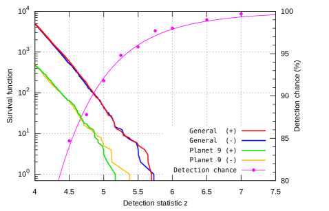
Figure 4: Left axis: Distribution of candidate detections for the Planet 9-like (green) and general (red) search compared to sign-flipped versions of the same searches (blue and yellow respectively), as a function of the detection statistic $z$. No signal is expected in the sign-flipped search, but it shares the same noise properties and many of the systematics (e.g., variable point sources and edge artifacts), so it gives a good estimate of the background detection rate. The lack of excess events in the positive curves vs. the negative ones (beyond the scatter expected from Poisson sample variance) means that we do not have any significant detections. Right axis: The probability of recovering an injected object as a function of $z$ (magenta). The detection probability is 95% by $z=5.3$.

We classified each candidate as Planet 9-like or general based on whether they satisfied the expected bounds on Planet 9’s orbital inclination, $10^{\circ}<i<30^{\circ}$ (B19). The inclination is not one of the free parameters of our fit, but we can approximate this selection by transforming the candidate coordinates and velocities into ecliptic coordinates, and requiring

$$\quad 10^{\circ} <\hat{i}<30^{\circ} \hat{i} =\sqrt{\beta^{2}+v_{\beta}^{2}/v_{\lambda}^{2}}$$ , (26)

and where $\lambda,\beta$ are the ecliptic longitude and latitude respectively, and $v_{\lambda},v_{\beta}$ are the velocity components in those directions. The formula for $\hat{i}$ assumes that orbits have $\beta(\lambda)=i\sin(\lambda-\lambda_{0})$, which is a decent approximation as long as $i$ is small.

Finally, the top 100 from each list were visually inspected using both the $z$ maps, the best-fit shift-stacked maps, raw sky maps and individual 3-day matched filter maps, and any obvious problems like edge artifacts, uncut variable point sources etc. were cut.

4.9 Flux and distance limits

It is useful to be able to translate the survey depth into detection limit maps. To do this, we need the false negative rate as a function of the detection statistic $z$. We found this by repeating the signal injection, search and detection procedure from Section 4.6 with two two important differences:

1. Simulated sources were added to the data instead of replacing it, resulting in noisy simulations.

2. For each simulated source we chose a target $z\in$ {4.50, 4.75, 5.00, 5.25, 5.50, 5.75, 6.00, 6.50, 7.00, 8.00, 10.00, 15.00}, translated this into a S/N ratio using $\xi^{-1}(z)$ (see Section 4.7 and Appendix B), and combined it with the local survey depth to define a simulated flux density $s=\xi^{-1}(z)/\sqrt{\kappa_{\text{tot}}^{\text{debiased}}}$.

We then ran the standard mean sky subtraction and candiate search on the maps, and computed the fraction of the injected sources that were ultimately recovered as a function of $z$. The result is plotted as the curve “detection chance” in Figure 4. Overall we find that a source bright enough to correspond to $z=5.3$ has a 95% chance of being detected. Hence, the 95% flux density detection limit map is given by

$$s_{\text{lim}}^{95\%} =\xi^{-1}(5.3)/\sqrt{\kappa_{\text{tot}}^{\text{debiased}}}$$ (27)

Aside from its position-dependence this limit is also distance-dependent, since both $\xi$ and $\kappa_{\text{tot}}^{\text{debiased}}$ depend on $r$.

Given a model for Planet 9’s luminosity we can translate the flux density limit to a distance limit. Since the flux density falls with the square of the distance, the distance limit $r_{\text{lim}}^{95\%}$ can be found as the solution to the equation

$$(r_{\text{ref}}/r)^{2}s_{\text{ref}} =s_{\text{lim}}^{95\%}(r_{\text{lim}})$$ (28)

with Table 1 showing examples of the reference flux $s_{\text{ref}}$ for $r_{\text{ref}}=500$ AU for different Planet 9 scenarios.

5 Results

The search resulted in 38 000 raw candidates, of which 3 500 and 35 000 fell into the Planet 9-like and general categories respectively. Manual inspection of the top 100 candidates led to 3 Planet 9-like and 17 general candidates being cut. These included the first three transients detected by ACT, which were published in a separate paper (Naess et al., 2020b). The top ten candidates from the Planet 9-like and general searches are shown in Tables 3 and 4. The full candidate distribution is shown in Figure 4 and is identical to within sample variance for both the normal and sign-inverted searches. The lack of excess events in the distribution of normal candidates vs. sign-inverted candidates means that we have no statistically significant detections.

Given our non-detection, we constrain the flux density from Planet 9 or similar objects in the outer solar system to be <4–12 mJy (95% confidence) for $r\geq 300\text{ AU}$ inside our survey area, depending on local survey depth. This limit is approximately distance-independent in the range $300\text{ AU}\leq r\leq 600\text{ AU}$, after which it gradually worsens to <5–15 mJy by 1500 AU. We show a map of the flux density limit in Figure 5, along with the locations of the top 10 candidates from the Planet 9-like and general searches.

Figure 6 shows the corresponding distance limits for the nominal $5M_{\earth}$ and $10M_{\earth}$ scenarios from Section 2. In the shallower parts of our survey area, a $5M_{\earth}$ Planet 9 would need to be more distant than 325 AU to evade detection. This increases to 625 AU in the deepest parts of our survey. For a $10M_{\earth}$ planet these numbers increase to 425 AU and 775 AU respectively.

We cover quite low galactic latitudes, but parts of the galaxy is still masked. This is usually confined to $|b|<2.5^{\circ}$, but it is not uncommon for the mask to extend beyond this to cover features like the Orion Nebula.

#	z map	Stack	f090	f150	RA	Dec	$\boldsymbol{z}$	F	$\boldsymbol{\Delta}$F	$\boldsymbol{r}$	$\boldsymbol{v_{x}}$	$\boldsymbol{v_{y}}$
					(∘)	(∘)		(mJy)	(mJy)	(AU)	(′/yr)	(′/yr)
1					-167.54	1.04	5.17	8.3	1.8	375	2.2	-2.9
2					-50.84	-9.16	5.05	11.5	2.4	375	0.2	3.0
3					-70.32	0.34	5.00	14.8	3.1	321	0.6	4.5
4					-150.37	-4.86	5.00	23.2	5.5	643	-0.1	-1.1
5					-179.17	-0.23	4.98	8.5	1.9	1125	0.0	0.4
6					179.01	4.34	4.92	6.3	1.4	500	1.3	-1.8
7					-173.55	15.20	4.92	4.1	0.9	346	-0.7	4.1
8					5.25	-0.70	4.87	5.6	1.3	643	-0.1	1.3
9					52.66	-2.60	4.87	10.1	2.3	563	-0.2	-1.7
10					-42.35	-45.80	4.87	8.4	1.7	500	0.3	1.8

Table 3: Top 10 Planet9-like candidates, sorted by the detection statistic $z$ (see Section 4.7 or Appendix B for definition). The columns are: #: The rank in terms of peak $z$ value. z map: A thumbnail of the $z$ map centered on the candidate. Stack: The shift-and-stack (i.e. motion-corrected) map for the best-fit parameters. f090/f150: Filtered versions of the mean sky model in the f090/f150 band. Because these do not include any motion correction, no Planet 9 signal is expected here, but they are useful for seeing how “clean” each candidate’s neighborhood is, e.g. if there are any bright point sources, dust clumps or map edges at or near the candidate’s location. All thumbnails are $45^{\prime}\times 45^{\prime}$ centered on the candidates. RA, Dec: Candidate’s J2000 heliocentric equatorial coordinates on modified Julian day (MJD) 57688. z: The candidate’s detection statistic $z$. F, $\Delta$F: Flux in the f150 band in mJy, assuming a 40 K blackbody, and its uncertainty. r: Distance from the Sun, in AU. $\boldsymbol{v_{x}}$, $\boldsymbol{v_{y}}$: Intrinsic motion in arcmin per year.

#	z map	Stack	f090	f150	RA	Dec	$\boldsymbol{z}$	F	$\boldsymbol{\Delta}$F	$\boldsymbol{r}$	$\boldsymbol{v_{x}}$	$\boldsymbol{v_{y}}$
					(∘)	(∘)		(mJy)	(mJy)	(AU)	(′/yr)	(′/yr)
1					-162.40	12.65	5.65	4.4	0.8	300	0.7	5.9
2					94.55	-29.48	5.64	9.7	1.8	500	1.6	1.5
3					116.58	-46.50	5.60	25.1	4.3	300	4.3	4.3
4					36.91	-12.81	5.51	13.7	3.4	1500	0.0	-0.1
5					59.20	1.52	5.48	11.3	2.4	643	0.6	0.6
6					69.03	-21.10	5.40	9.0	1.7	300	3.9	1.4
7					179.90	13.94	5.28	4.8	0.9	346	-3.7	-2.3
8					-8.19	-17.78	5.28	12.1	2.8	1125	-0.3	0.0
9					-69.90	-19.31	5.15	14.9	4.4	2000	0.0	0.1
10					-102.24	13.04	5.14	6.5	1.4	500	-1.4	-1.6

Table 4: Like Table 3, but for the general candidates.

$300<r<600$ AU
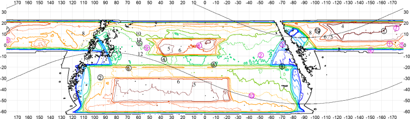
$r=1500$ AU

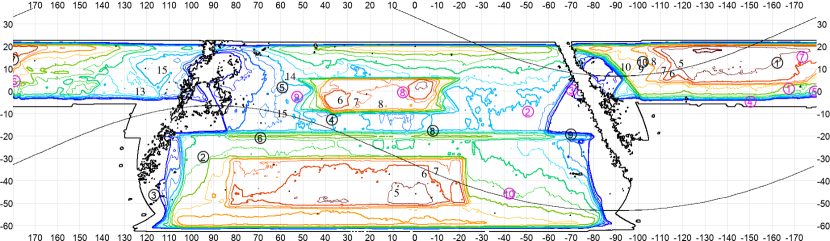
Figure 5: Flux limit for the general Planet 9 search for distance $300<r<600$ AU (top) and $r=2000$ AU (bottom) in equatorial coordinates. Objects brighter than this would be part of our top-10 candidate list. The contours go from red (4 mJy) to blue (20 mJy) in steps of 1 mJy. Some individual contour lines are labeled (plain black numbers) with their corresponding depth, for convenience. The flux density limit depends on the size of the parameter search space, which shrinks with $r$ leading to a lower flux density limit; and the loss from mean sky subtraction, which raises the flux density limit. These effects mostly balance each other for $300<r<600$, while the mean sky subtraction loss dominates at higher $r$, leading to a gradually increasing flux density limit. The circled numbers show the locations of the top-10 candidates from the general (black) and Planet 9-like (magenta) searches. The thin black curves delimit the area with inclination less than 30^∘. The point source mask was left out from this plot, but its effect can be seen in Figure 6.

$5M_{\earth}$ (250–625 AU)
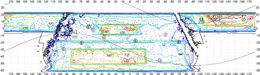
$10M_{\earth}$ (350–775 AU)

Figure 6: Top: Distance limit for detection of a $5M_{\earth}$ Planet 9 with the nominal composition from Section 2. Contours go from 250 AU (blue) to 550 AU (red) in steps of 25 AU, with some contours labeled for convenience. Note that $r<300$ AU were not included in the search, so areas with a distance limit $\lesssim 300$ AU do not meaningfully constrain Planet 9. The circled numbers show the locations of the top-10 candidates from the general (black) and Planet 9-like (magenta) searches. The little colored dots are caused by the point source mask. Its effect appears exaggerated because of the low resolution of the plot – in reality this mask only affects a tiny fraction of the sky. Bottom: As above, but for a $10M_{\earth}$ Planet 9. The contours here go from 350 AU (blue) to 750 AU (red).

$5M_{\earth}$	$10M_{\earth}$

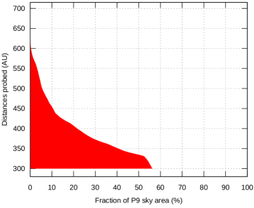
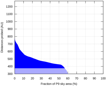
Figure 7: Our Planet 9 exclusion limit distribution with the nominal composition from section 2, showing what distance range we can exclude over a given fraction of the Planet 9 expected sky area ($|\beta|<30^{\circ}$). The value on the x axis gives the fraction of the Planet 9 sky area where our bounds are at least as good as the distance given on the y axis. This is what one gets if one sorts the values in Figure 6 in descending order. Left: The nominal $5M_{\earth}$ Planet 9 is predicted to be between roughly 280 AU and 715 AU distant (see Table 2). This curve shows that we are sensitive up to 600 AU over a few percent of the Planet 9 sky area; up to 450 AU over 10% of that area; 300 AU to at least 350 AU over 40% of the area; and so on. The colored fraction of the graph gives a rough idea of what fraction of the Planet 9 parameter space we probe. Right: As left, but for the $10M_{\earth}$ version of the planet. The light shaded region represents distances we probe that are closer than what is allowed by the prior.

$5M_{\earth}$

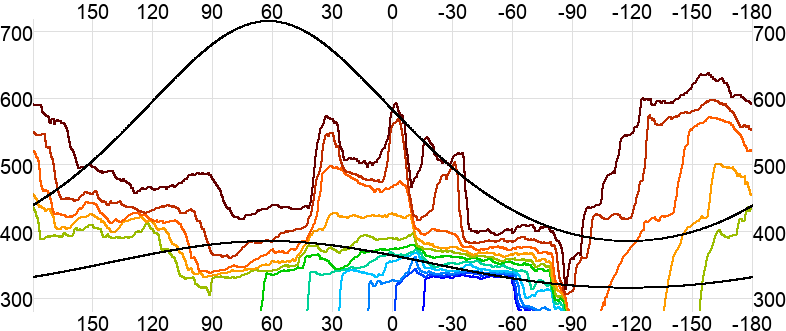
$10M_{\earth}$

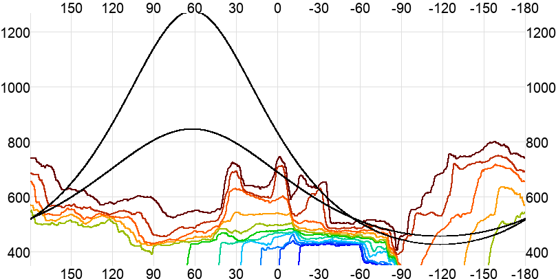
Figure 8: Distance limit distribution as a function of ecliptic longitude compared to the Planet 9 orbit. The x axis is ecliptic longitude in degrees. The y axis is the planet’s current distance from the Sun. The colored curves are deciles of the distance limit distribution for the Planet 9-like search, from blue (0%) to red (100%). The bottom and top black curves represent respectively a low-$a$, low-$e$ case and a high-$a$, high-$e$ case. These roughly bracket the Planet 9 prior space, though they keep the aphelion fixed at RA = $60^{\circ}$ ($\beta=62^{\circ}$) instead of marginalizing over it. When a black curve is below the bluest curve, then all pixels at that longitude are deep enough to detect it. When the black curve is above the reddest curve, then no pixels at that longitude are deep enough to detect it. And when the black curve crosses the 70% quantile (orange), then 70% of the pixels are too shallow to detect it. The top and bottom panels are for a $5M_{\earth}$ (low: $a=350\text{AU}$, $e=0.1$; high: $a=550\text{AU}$, $e=0.3$) and $10M_{\earth}$ (low: $a=650\text{AU}$, $e=0.3$; high: $a=850\text{AU}$, $e=0.5$) Planet 9 respectively.

6 Discussion

As the possible signal curves in Figure 1 showed, ACT’s non-detection is not surprising, especially considering that a planet in an eccentric orbit moves more slowly near aphelion, and is therefore more likely to be located there. Planet 9’s aphelion is predicted to be around $\text{RA}\approx 60^{\circ}$, an area where the ACT coverage is quite shallow, corresponding to a $5M_{e}$ detection limit of about 350 AU. For comparison, the smallest expected aphelion distance is a bit less than 400 AU (Table 2). Hence, at its current depth, ACT can not expect to see Planet 9 if it is near aphelion.

Because B19 does not provide a well-defined prior volume, it is hard to quantify what fraction of the Planet 9 parameter space we have probed, but we can make a few simple estimates. Figure 7 shows the distribution of our distance limits for the Planet 9-relevant parts of the sky ($|i|<30^{\circ}$), and compares them to the $\sim$ 300–700 AU and $\sim$ 400–1300 AU allowed distance range for a $5M_{\earth}$ and $10M_{\earth}$ Planet 9 respectively. We probe about 13% and 8% of this distance-position space. However, that does not take into account the fact that the furthest Planet 9 distances are only expected to occur in some parts of the sky. The spatial dependence of the predicted Planet 9 distance range is shown in Figure 8, and taking it into account, our numbers improve to 17% and 9% respectively.

The upcoming Simons Observatory (SO) (SO Collaboration, 2019) will substantially improve on these bounds. Extrapolating our current results to the expected depth of the combined ACT+SO data set, we can expect to detect a $5M_{\earth}$ Planet 9 at 500–600 AU near the expected aphelion location and 500–900 AU over most of the rest of its orbit. This is still not enough to guarantee a discovery, but it will probe a substantial fraction of its parameter space. Unlike bounds from optical surveys like Pan-STARRS and LSST, and even sub-mm ones like WISE, the ACT and SO searches are only mildly sensitive to Planet 9’s physical composition, and are robust to assumptions about atmospheric emission lines and albedo.

Appendix A Smearing

A.1 Circular smearing

Consider a Gaussian beam with standard deviation $\sigma$, such that its profile is

$$b(r) =e^{-\frac{1}{2}\frac{r^{2}}{\sigma^{2}}}=e^{-\frac{1}{2}\frac{x^{2}+y^{2}}{\sigma^{2}}}$$ (A1)

where $r=\sqrt{x^{2}+y^{2}}$. Partially uncorrected parallax smears this beam along an ellipse with some semi-major axis $\mu$. The simplest and worst case of this is smearing along a circle with radius $\mu$, so that’s what we will consider here. This results in the smeared beam

$$b_{2}(r,\mu) =\frac{1}{2\pi}\int_{0}^{2\pi}d\theta e^{-\frac{1}{2}\frac{(x-\mu\cos\theta)^{2}+(y-\mu\sin\theta)^{2}}{\sigma^{2}}}\propto b(r)\int_{0}^{2\pi}d\theta e^{\frac{x\mu\cos\theta+y\mu\sin\theta}{\sigma^{2}}}$$

$$\approx b(r)\int_{0}^{2\pi}d\theta\left(1+\frac{x\mu\cos\theta+y\mu\sin\theta}{\sigma^{2}}+\frac{1}{2}\left(\frac{x\mu\cos\theta+y\mu\sin\theta}{\sigma^{2}}\right)^{2}\right)$$

$$\propto b(r)\left(1+\frac{1}{4}\frac{r^{2}\mu^{2}}{\sigma^{4}}\right)$$ (A2)

where we have assumed $\mu\ll\sigma$ and have ignored any factors that just scale the overall amplitude of the function. If all values $\mu\in[-\frac{\Delta}{2},\frac{\Delta}{2}]$ occur with equal weight, then the average beam across all these will be:

$$b_{\text{eff}}(r) =\frac{1}{\Delta}\int_{-\frac{\Delta}{2}}^{\frac{\Delta}{2}}d\mu b_{2}(r,\mu)=\frac{1}{\Delta}b(r)\int_{-\frac{\Delta}{2}}^{\frac{\Delta}{2}}d\mu\left(1+\frac{1}{4}\frac{r^{2}\mu^{2}}{\sigma^{4}}\right)=b(r)\left(1+\frac{1}{24}\frac{r^{2}\Delta^{2}}{\sigma^{4}}\right)\approx e^{-\frac{1}{2}\frac{r^{2}}{\sigma^{2}}}e^{\frac{1}{24}\frac{r^{2}\Delta^{2}}{\sigma^{4}}}=e^{-\frac{1}{2}\frac{r^{2}}{\sigma_{\text{eff}}^{2}}}$$ (A3)

where

$$\sigma_{\text{eff}}^{2} =\frac{\sigma^{2}}{1-\frac{1}{12}\frac{\Delta^{2}}{\sigma^{2}}}\approx\sigma^{2}+\frac{1}{12}\Delta^{2}\quad\Leftrightarrow\quad\text{FWHM}_{\text{eff}}^{2}=\text{FWHM}^{2}+\frac{2\log(2)}{3}\Delta^{2}$$ (A4)

So circular smearing adds in quadrature to the beam size.

A.2 Linear smearing

We here smear the beam linearly in the x direction with $\mu\in[-\frac{\Delta}{2},\frac{\Delta}{2}]$.

$$b_{\text{eff}} =\frac{1}{\Delta}\int_{-\frac{\Delta}{2}}^{\frac{\Delta 2}{d}}\mu e^{-\frac{1}{2}\frac{(x-\mu)^{2}+y^{2}}{\sigma^{2}}}\approx b(r)\int_{-\frac{\Delta}{2}}^{\frac{\Delta}{2}}d\mu\left(1+\frac{x\mu}{\sigma^{2}}+\frac{1}{2}\frac{x^{2}\mu^{2}}{\sigma^{4}}\right)\frac{e^{-\frac{1}{2}\frac{\mu^{2}}{\sigma^{2}}}}{\Delta}\propto b(r)\left(1+\frac{1}{12}\frac{x^{2}\Delta^{2}}{\sigma^{4}}\right)\approx e^{-\frac{1}{2}\left(\frac{x^{2}}{\sigma_{x,\text{eff}}}+\frac{y^{2}}{\sigma^{2}}\right)}$$ (A5)

with $\sigma_{x,\text{eff}}^{2}=\sigma^{2}+\frac{1}{6}\Delta^{2}$. Since only the x direction was smeared, the beam is now slightly elliptical. For the purposes of S/N, what matters is not the shape of the beam, but its area, which has gone from $2\pi\sigma^{2}$ to $2\pi\sigma\sigma_{x,\text{eff}}$. We can use this to define an effective overall beam standard deviation:

$$\sigma_{\text{eff}}^{2} =\sigma\sigma_{x,\text{eff}}=\sigma^{2}\sqrt{1+\frac{1}{6}\frac{\Delta^{2}}{\sigma^{2}}}\approx\sigma^{2}+\frac{1}{12}\Delta^{2}\quad\Leftrightarrow\quad\text{FWHM}_{\text{eff}}^{2}=\text{FWHM}^{2}+\frac{2\log(2)}{3}\Delta^{2}$$ (A6)

Which happens to be the same result as what we got for circular smearing.

Appendix B Building the detection statistic $z$

The S/N map produced by the shift-and-stack search is non-Gaussian with properties that depend on both the distance $r$ and the position in the map, making it unsuitable as an indication of the detection strength. However, we found that the following three-step approach allowed us to transform $S/N$ into a much more well-behaved detection statistic $z$.

B.1 Spatial normalization

Raw	Normalized

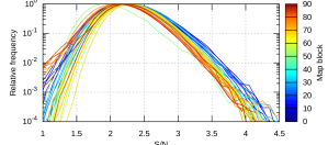
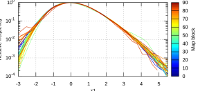
Figure 9: Spatial normalization of the detection statistic. Left: Histograms for the shift-and-stack S/N ratio for the 300 AU case. Each curve corresponds to a different $5^{\circ}\times 5^{\circ}$ part of the map. The distribution is non-Gaussian and spatially variable. Right: The same histograms after normalizing by subtracting the mean and dividing by the standard deviation. After this the distribution is no longer spatially variable. The actual spatial normalization used in the search uses smaller $0.5^{\circ}\times 4^{\circ}$ degree tiles, which are large enough to measure the mean and standard deviation reliably, but result in noisier histograms.

For each $r$ we measure the mean $\mu_{\text{spat}}(r)$ and standard deviation $\sigma_{\text{spat}}(r)$ of the S/N map as a function of position. Using these, we define the spatially-normalized detection statistic $z_{1}$ as

$$z_{1}(r) =[S/N(r)-\mu_{\text{spat}}(r)]/\sigma_{\text{spat}}(r)$$ (B1)

This normalization process is shown in Figure 9.

B.2 Distance normalization

$z_{1}$ survival function	$z_{1}$ vs $z^{*}$
$z$ survival function	$z$ vs $z^{*}$

Figure 10: Distance normalization of the detection statistic. Top left: The tail of the survival function of $z_{1}$. Each color corresponds to a different distance bin, from 300 AU (blue) to 2000 AU (red). The different distances clearly do not follow the same distribution. Top right: As top left, but with the survival function replaced with the corresponding Gaussian quantile $z^{*}$. For each distance we define $\mu_{\text{dist}}$ and $\sigma_{\text{dist}}$ as the best-fit linear offset and slope of its curve. Bottom left: The survival function for the distance-normalized detection statistic $z=(z_{1}-\mu_{\text{dist}})/\sigma_{\text{dist}}$. All distances now follow the same distribution. Bottom right: $z$ vs. the empirical Gaussian quantiles $z^{*}$. They are practically identical.

We then build the empirical survival function $N(z_{1}>x)$ for all peaks in the tile with $z_{1}>1$ and map this to a corresponding Gaussian quantile

$$z^{*}=-\sqrt{2}\text{ erf}^{-1}(2N/n-1)$$ (B2)

The value of $n$ controls how far into the tail of a Gaussian survival function we map our empirical survival function. Its exact value is not important as long as $n>\text{max}(N)$. It should be kept constant for all values of $r$ to ensure that equally rare values of $z_{1}$ map to the same $z^{*}$ for all distances. We chose $n=A_{\text{tile}}/A_{\text{peak}}\approx(12^{\circ}/2^{\prime})^{2}=1.3\cdot 10^{6}$, with $A_{\text{tile}}=(12^{\circ})^{2}$ being the area of the tile, and $A_{\text{peak}}=(2^{\prime})^{2}$ being the approximate feature size in the $z_{1}$ map. In principle eq. B2 could be used to directly normalize $z_{1}$, but in practice there are too few samples in the tail. However, $z^{*}$ turns out to be very well approximated as a linear function of $z_{1}$. We use this to define the fully normalized detection statistic

$$z(r) =[z_{1}(r)-\mu_{\text{dist}}(r)]/\sigma_{\text{dist}}(r)$$ (B3)

where $\mu_{\text{dist}}$ and $\sigma_{\text{dist}}$ are the offset and slope of the function $z^{*}(z_{1})$. This process is illustrated in Figure 10. Inserting the expression for $z_{1}$ into equation B3, we get the full normalization

$$z(r) =(S/N(r)-\mu_{z}(r))/\sigma_{z}(r)=\xi(S/N)$$ (B4)

where we have defined $\mu_{z}=\mu_{\text{spat}}+\sigma_{\text{spat}}\mu_{\text{dist}}$ and $\sigma_{z}=\sigma_{\text{spat}}\sigma_{\text{dist}}$; and we have implicitly defined the function $\xi$.

Appendix C Ad-hoc filter

The map noise power can be approximately modeled as $1/\beta(\ell,\ell_{\text{knee}},\alpha)$, where $\beta$ is the Butterworth filter profile

$$\beta(\ell,\ell_{\text{knee}},\alpha)=1/[1+(\ell/\ell_{\text{knee}})^{\alpha}]$$ (C1)

This noise power spectrum takes the form of a power law with slope $\alpha\approx-4$ at low $\ell$ (mainly caused by atmospheric emission) which transitions to a flat “noise floor” around the multipole $\ell_{\text{knee}}\approx 3000$ where photon noise and detector readout noise start to dominate. However, it turned out that $N$, the noise model we use for our time-ordered data analysis (see eq. 5) does not capture the full correlation structure of the atmosphere, and ends up underestimating the effective $\ell_{\text{knee}}$ by a factor of two, i.e. $\ell_{\text{knee}}^{\prime}\approx 1500$. This means that our matched filter did not suppress noise in the $1500\lesssim\ell\lesssim 3000$ range as much as it should be, leading to a loss in S/N.

To correct for this, we replace the map inverse covariance matrix $U^{-1}$ with $\beta(\ell,3000,-4)U^{-1}$. Accordingly $\rho=R^{T}U^{-1}\hat{m}$ is remapped at $\rho\rightarrow\beta\rho$. What happens to $\kappa=\text{diag}(R^{T}U^{-1}R)$ is harder to estimate. We can approximate it as $\kappa\rightarrow q\kappa$, where $q$ a single number representing the weighted average of the extra filter $\beta(\ell,3000,-4)$ over all multipoles,

$$q=\frac{\sum_{\ell}(2\ell+1)W(\ell)\beta(\ell,3000,-4)}{\sum_{\ell}(2\ell+1)W_{\ell}}$$ (C2)

with the weights $W(\ell)$ being a harmonic-space approximation of the original matched filter,

$$W(\ell) =\beta(\ell,1500,-4)B(\ell)$$ (C3)

where $B(\ell)$ is the beam and $\beta(\ell,1500,-4)$ approximates the original $U^{-1}$. However, in the end the normalization of $\kappa$ does not matter, since it is absorbed by the simulation-based debiasing we do to account for the effect of mean sky subtraction in Section 4.6.

The ad-hoc filter could have been avoided if we had computed the full $\hat{m}$ and had done the full matched filter in pixel-space instead of using the “rhs” computational shortcut described in Section 4.3.4. This is a protential improvement for future analyses.

Appendix D ACT data set details

Table 5 summarizes the ACT data sets used in this analysis.

Survey	Patch	RA (∘)		dec (∘)		Data sets
ACT DR4	D1	140  –	161	-5  –	6	PA1 2013
ACT DR4	D5	-19  –	13	-7  –	6	PA1 2013
ACT DR4	D6	19  –	48	-11  –	1	PA1 2013
ACT DR4	D56	-23  –	54	-10  –	7	PA1+PA2 2014–2015, PA3 2015
ACT DR4	D8	-12  –	18	-52  –	-32	PA1+PA2+PA3 2015
ACT DR4	BN	102  –	257	-7  –	22	PA1+PA2+PA3 2015
ACT DR4	AA	0  –	360	-62  –	22	PA2+PA3 2016
AdvACT	AA	0  –	360	-62  –	22	PA4+PA5+PA6 2017–2019
ACT day	BN	102  –	257	-7  –	22	PA1+PA2 2014–2015, PA3 2015
ACT day	Day-N	162  –	258	3  –	20	PA2+PA3 2016, PA4+PA5+PA6 2017–2019
ACT day	Day-S	-25  –	60	-52  –	-29	PA4+PA5+PA6 2017–2019

Table 5: ACT data sets used in the analysis. They are identical to those used in ACT DR5 (Naess et al., 2020a), except for the inclusion of data from the 2019 observing season, and the exclusion of Planck (too low resolution) and ACT MBAC (too low sky coverage). PA{1-6} refers to the individual detector arrays in the instrument, with PA{1,2} covering the f150 band, PA{3,5,6} covering f090 and f150, and PA4 covering f150 and f220.

References

- AllWISE (2013) AllWISE. 2013, AllWISE explanatory supplement, https://wise2.ipac.caltech.edu/docs/release/allwise/expsup/sec2_1.html
- Astropy Collaboration (2013) Astropy Collaboration. 2013, arXiv:1307.6212, A&A, 558, A33, Astropy: A community Python package for astronomy
- Batygin et al. (2019) Batygin, K., Adams, F. C., Brown, M. E., & Becker, J. C. 2019, arXiv:1902.10103, Phys. Rep., 805, 1, The planet nine hypothesis
- Batygin & Brown (2016) Batygin, K. & Brown, M. E. 2016, AJ, 151, 22, Evidence for a distant giant planet in the solar system, http://dx.doi.org/10.3847/0004-6256/151/2/22
- Baxter et al. (2018) Baxter, E. J., Jain, B., Blake, C., Bernstein, G., Devlin, M., & Holder, G. 2018, arXiv:1812.08701, arXiv e-prints, arXiv:1812.08701, Planet X in CMB and Optical Galaxy Surveys
- Bernardinelli et al. (2020) Bernardinelli, P. H., et al. 2020, PSJ, 1, 28, Testing the Isotropy of the Dark Energy Survey’s Extreme Trans-Neptunian Objects, http://dx.doi.org/10.3847/PSJ/ab9d80
- Brown (2021) Brown, M. 2021, https://findplanetnine.blogspot.com/2021/02/is-planet-nine-finally-dead.html
- Carlstrom et al. (2011) Carlstrom, J. E., et al. 2011, arXiv:0907.4445, PASP, 123, 568, The 10 Meter South Pole Telescope
- Chambers et al. (2016) Chambers, K. C., et al. 2016, arXiv:1612.05560, arXiv e-prints, arXiv:1612.05560, The Pan-STARRS1 Surveys
- Choi et al. (2018) Choi, S. K., et al. 2018, arXiv:1711.04841, JLTP, 193, 267, Characterization of the Mid-Frequency Arrays for Advanced ACTPol
- Choi et al. (2020) —. 2020, arXiv:1908.10451, JLTP, 199, 1089, Sensitivity of the Prime-Cam Instrument on the CCAT-Prime Telescope
- Cowan et al. (2016) Cowan, N. B., Holder, G., & Kaib, N. A. 2016, arXiv:1602.05963, ApJ, 822, L2, Cosmologists in Search of Planet Nine: The Case for CMB Experiments
- Fortney et al. (2016) Fortney, J. J., et al. 2016, arXiv:1604.07424, AJ, 824, L25, The hunt for Planet Nine: Atmosphere, Spectra, Evolution, and Detectability, http://dx.doi.org/10.3847/2041-8205/824/2/L25
- Fowler et al. (2007) Fowler, J. W., et al. 2007, astro-ph/0701020, Appl. Opt., 46, 3444, Optical design of the Atacama Cosmology Telescope and the Millimeter Bolometric Array Camera
- Gladman et al. (1998) Gladman, B., Kavelaars, J. J., Nicholson, P. D., Loredo, T. J., & Burns, J. A. 1998, astro-ph/9806344, AJ, 116, 2042, Pencil-Beam Surveys for Faint Trans-Neptunian Objects
- Górski et al. (2005) Górski, K. M., Hivon, E., Banday, A. J., Wandelt, B. D., Hansen, F. K., Reinecke, M., & Bartelmann, M. 2005, arXiv:astro-ph/0409513, ApJ, 622, 759, HEALPix: A Framework for High-Resolution Discretization and Fast Analysis of Data Distributed on the Sphere
- Ho et al. (2017) Ho, S.-P. P., et al. 2017, in Proc. SPIE, Vol. 9914, Millimeter, Submillimeter, and Far-Infrared Detectors and Instrumentation for Astronomy VIII, 991418, https://act.princeton.edu/sites/act/files/highly_uniform_150mm.pdf
- Holman et al. (2018) Holman, M. J., Payne, M. J., Blankley, P., Janssen, R., & Kuindersma, S. 2018, arXiv:1805.02638, arXiv e-prints, arXiv:1805.02638, Finding Asteroids Down the Back of the Couch: A Novel Approach to the Minor Planet Linking Problem
- Hunter (2007) Hunter, J. D. 2007, Computing in Science & Engineering, 9, 90, Matplotlib: A 2D graphics environment
- Ishihara et al. (2010) Ishihara, D., et al. 2010, arXiv:1003.0270, A&A, 514, A1, The AKARI/IRC mid-infrared all-sky survey
- Ivezić et al. (2019) Ivezić, Ž., et al. 2019, arXiv:0805.2366, ApJ, 873, 111, LSST: From Science Drivers to Reference Design and Anticipated Data Products
- Luhman (2013) Luhman, K. L. 2013, ApJ, 781, 4, A search for a distant companion to the Sun with the Wide-Field Infrared Survey Explorer, https://doi.org/10.1088/0004-637x/781/1/4
- Meisner et al. (2018) Meisner, A. M., Bromley, B. C., Kenyon, S. J., & Anderson, T. E. 2018, arXiv:1712.04950, AJ, 155, 166, A 3 Search for Planet Nine at 3.4 m with WISE and NEOWISE
- Naess et al. (2020a) Naess, S., et al. 2020a, arXiv:2007.07290, J. Cosmology Astropart. Phys, 2020, 046, The Atacama Cosmology Telescope: arcminute-resolution maps of 18 000 square degrees of the microwave sky from ACT 2008-2018 data combined with Planck
- Naess et al. (2020b) —. 2020b, arXiv:2012.14347, arXiv e-prints, arXiv:2012.14347, The Atacama Cosmology Telescope: Detection of mm-wave transient sources
- Napier et al. (2021) Napier, K. J., et al. 2021, arXiv:2102.05601, PSJ, 2, 59, No Evidence for Orbital Clustering in the Extreme Trans-Neptunian Objects
- Pan-STARRS (2015) Pan-STARRS. 2015, https://star.pst.qub.ac.uk/ps1threepi/psdb/
- Price-Whelan et al. (2018) Price-Whelan, A. M., et al. 2018, AJ, 156, 123, The Astropy Project: Building an Open-science Project and Status of the v2.0 Core Package
- Schlafly et al. (2019) Schlafly, E. F., Meisner, A. M., & Green, G. M. 2019, arXiv:1901.03337, ApJS, 240, 30, The unWISE Catalog: Two Billion Infrared Sources from Five Years of WISE Imaging
- Shankman et al. (2017) Shankman, C., et al. 2017, AJ, 154, 50, OSSOS. VI. Striking Biases in the Detection of Large Semimajor Axis Trans-Neptunian Objects, http://dx.doi.org/10.3847/1538-3881/aa7aed
- SO Collaboration (2019) SO Collaboration. 2019, JCAP, 2019, 056–056, The Simons Observatory: science goals and forecasts, http://dx.doi.org/10.1088/1475-7516/2019/02/056
- Thornton et al. (2016) Thornton, R. J., et al. 2016, arXiv:1605.06569, ApJS, 227, 21, The Atacama Cosmology Telescope: The Polarization-sensitive ACTPol Instrument
- W.G. (1986) W.G., J. I. S. 1986, IRAS Catalog of Point Sources, Version 2.0, https://heasarc.gsfc.nasa.gov/W3Browse/iras/iraspsc.html
- Yamamura et al. (2010) Yamamura, I., Makiuti, S., Ikeda, Y., Oyabu, S., Koga, T., & White, G. J. 2010, AKARI/FIS All-Sky Survey Bright Source Catalogue Version 1.0 Release Note, https://irsa.ipac.caltech.edu/data/AKARI/documentation/AKARI-FIS_BSC_V1_RN.pdf
- Zonca et al. (2019) Zonca, A., Singer, L., Lenz, D., Reinecke, M., Rosset, C., Hivon, E., & Gorski, K. 2019, JOSS, 4, 1298, healpy: equal area pixelization and spherical harmonics transforms for data on the sphere in Python, https://doi.org/10.21105/joss.01298