Outcome-Driven Reinforcement Learning via Variational Inference

   Tim G. J. Rudner  
University of Oxford
&  Vitchyr H. Pong
University of California, Berkeley
Rowan McAllister
University of California, Berkeley
&Yarin Gal
University of Oxford
&Sergey Levine
University of California, Berkeley
Equal contribution.  Corresponding authors: tim.rudner@cs.ox.ac.uk and vitchyr@berkeley.edu.
Abstract

While reinforcement learning algorithms provide automated acquisition of optimal policies, practical application of such methods requires a number of design decisions, such as manually designing reward functions that not only define the task, but also provide sufficient shaping to accomplish it. In this paper, we view reinforcement learning as inferring policies that achieve desired outcomes, rather than as a problem of maximizing rewards. To solve this inference problem, we establish a novel variational inference formulation that allows us to derive a well-shaped reward function which can be learned directly from environment interactions. From the corresponding variational objective, we also derive a new probabilistic Bellman backup operator and use it to develop an off-policy algorithm to solve goal-directed tasks. We empirically demonstrate that this method eliminates the need to hand-craft reward functions for a suite of diverse manipulation and locomotion tasks and leads to effective goal-directed behaviors.

1 Introduction

Reinforcement learning (RL) provides an appealing formalism for automated learning of behavioral skills, but requires considerable care and manual design to use in practice. One particularly delicate decision is the design of the reward function, which has a significant impact on the resulting policy but is largely heuristic in practice, often lacks theoretical grounding, can make effective learning difficult, and may lead to reward mis-specification.

To avoid these shortcomings, we propose to circumvent the process of manually specifying a reward function altogether: Instead of framing the reinforcement learning problem as finding a policy that maximizes a heuristically-defined reward function, we express it probabilistically, as inferring a state–action trajectory distribution conditioned on a desired future outcome. By building off of prior work on probabilistic perspectives on RL [10, 23, 35, 46, 47, 58] and goal-directed RL in particular [3, 6, 19, 48], we derive a tractable variational objective, an temporal-difference algorithm that provides a shaping-like effect for effective learning, as well as a reward function that captures the semantics of the underlying decision problem and facilitates effective learning.

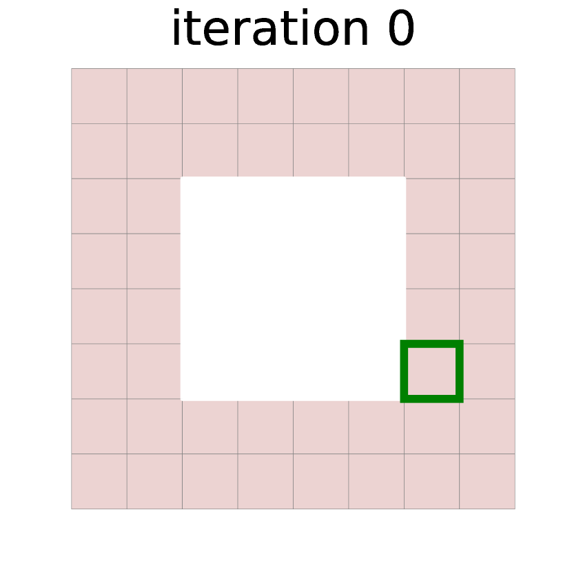
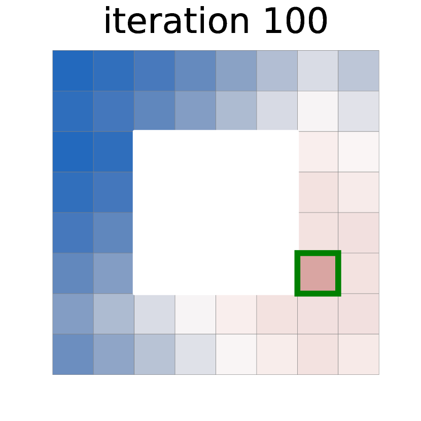
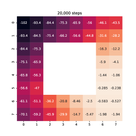
We demonstrate that unlike prior works that proposed inference methods for finding policies that achieve desired outcomes [3, 11, 19, 48], the resulting algorithm, Outcome-Driven Actor–Critic (odac), is amenable to off-policy learning and applicable to complex, high-dimensional continuous control tasks over finite and infinite horizons. The resulting variational algorithm can be interpreted as an automatic shaping method, where each iteration learns a reward function that automatically provides dense rewards, as we visualize in Figure 1. In tabular settings, odac is guaranteed to converge to an optimal policy, and in non-tabular settings with linear Gaussian transition dynamics, the derived optimization objective is convex in the policy, facilitating easier learning. In high-dimensional and non-linear domains, our method can be combined with deep neural network function approximators to yield a deep reinforcement learning method that does not require manual specification of rewards, and leads to good performance on a range of benchmark tasks.

Contributions.

The core contributions of this paper are the probabilistic formulation of a general framework for inferring policies that lead to desired outcomes and the derivation of a variational objective from which we obtain a novel outcome-driven Bellman backup operator. We show that this Bellman backup operator induces a shaping-like effect which ensures a clear and dense learning signal even in the early stages of training. Crucially, unlike heuristic approaches for incorporating shaping often used in standard RL, this “shaping” emerges automatically from variational inference. We demonstrate that the resulting variational objective is a lower bound on the log-marginal likelihood of achieving the outcome given an initial state and that it leads to an off-policy temporal-difference algorithm. We evaluate this algorithm—Outcome-Driven Variational Inference (odac)—on a range of reinforcement learning tasks without having to manually specify task-specific reward functions. In our experiments, we find that our method results in significantly faster learning across a variety of robot manipulation and locomotion tasks than alternative approaches.

Refer to caption
Refer to caption
Refer to caption
Refer to caption
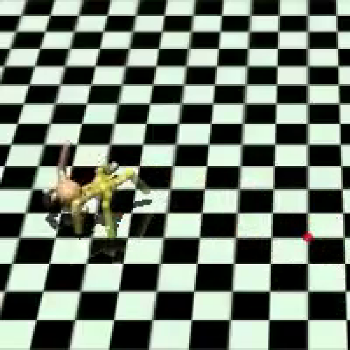
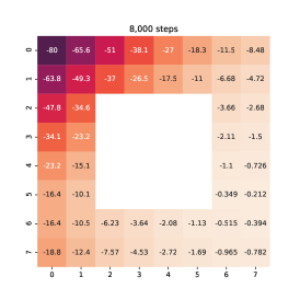
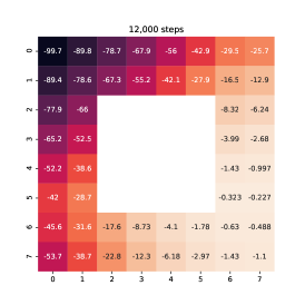
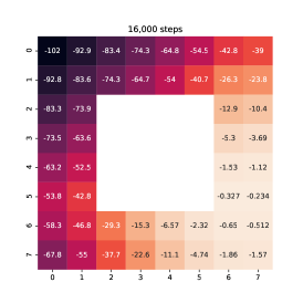
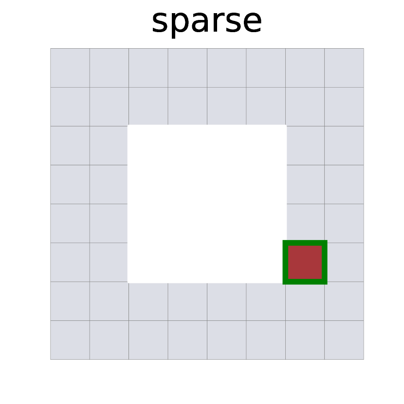
Figure 1: Illustration of the shaping effect of the reward function derived from the goal-directed variational inference objective. Left: A 2-dimensional grid world with a desired outcome marked by a star. Center-left The corresponding sparse reward function provides little shaping. Center-right: The reward function derived from our variational inference formulation at initialization. Right: The derived reward function after training. We see that the derived reward learns to provide a dense reward signal everywhere in the state space.

2 Preliminaries

Standard reinforcement learning (RL) addresses reward maximization in a Markov decision process (MDP) defined by the tuple (𝒮,𝒜,p𝐒0,pd,r,γ)𝒮𝒜subscript𝑝subscript𝐒0subscript𝑝𝑑𝑟𝛾(\mathcal{S},\mathcal{A},p_{\mathbf{S}_{0}},p_{d},r,\gamma) [43, 44], where 𝒮𝒮\mathcal{S} and 𝒜𝒜\mathcal{A} denote the state and action space, respectively, p0subscript𝑝0p_{0} denotes the initial state distribution, pdsubscript𝑝𝑑p_{d} is a state transition distribution, r𝑟r is an immediate reward function, and γ𝛾\gamma is a discount factor. To sample trajectories, an initial state is sampled according to p𝐒0subscript𝑝subscript𝐒0p_{\mathbf{S}_{0}}, and successive states are sampled from the state transition distribution 𝐒t+1pd(|𝐬t,𝐚t)\mathbf{S}_{t+1}\sim p_{d}(\cdot\,|\,\mathbf{s}_{t},\mathbf{a}_{t}) and actions from a policy 𝐀tπ(|𝐬t)\mathbf{A}_{t}\sim\pi(\cdot\,|\,\mathbf{s}_{t}). We will write 𝓣0:t={𝐒0,𝐀0,𝐒1,,𝐒t,𝐀t}subscript𝓣:0𝑡subscript𝐒0subscript𝐀0subscript𝐒1subscript𝐒𝑡subscript𝐀𝑡\bm{\mathcal{T}}_{0:t}=\{\mathbf{S}_{0},\mathbf{A}_{0},\mathbf{S}_{1},\dots,\mathbf{S}_{t},\mathbf{A}_{t}\} to represent a finite-horizon and 𝓣0=˙{𝐀t,𝐒t+1}t=0subscript𝓣0˙superscriptsubscriptsubscript𝐀𝑡subscript𝐒𝑡1𝑡0\bm{\mathcal{T}}_{0}\,\,\dot{=}\,\,\{\mathbf{A}_{t},\mathbf{S}_{t+1}\}_{t=0}^{\infty} to represent an infinite-horizon stochastic state–action trajectory, and write 𝝉0:t={𝐬0,𝐚0,𝐬1,,𝐬t,𝐚t}subscript𝝉:0𝑡subscript𝐬0subscript𝐚0subscript𝐬1subscript𝐬𝑡subscript𝐚𝑡\bm{\tau}_{0:t}=\{\mathbf{s}_{0},\mathbf{a}_{0},\mathbf{s}_{1},\dots,\mathbf{s}_{t},\mathbf{a}_{t}\} and 𝝉0=˙{𝐚t,𝐬t+1}t=0subscript𝝉0˙superscriptsubscriptsubscript𝐚𝑡subscript𝐬𝑡1𝑡0\bm{\tau}_{0}\,\,\dot{=}\,\,\{\mathbf{a}_{t},\mathbf{s}_{t+1}\}_{t=0}^{\infty} for the respective trajectory realizations. Given a reward function r:𝒮×𝒜:𝑟𝒮𝒜r:\mathcal{S}\times\mathcal{A}\to\mathbb{R} and discount factor γ(0,1)𝛾01\gamma\in(0,1), the objective in reinforcement learning is to find a policy π𝜋\pi that maximizes the returns, defined as 𝔼pπ[t=0γtr(𝐬t,𝐚t)],subscript𝔼subscript𝑝𝜋superscriptsubscript𝑡0superscript𝛾𝑡𝑟subscript𝐬𝑡subscript𝐚𝑡\operatorname{\mathbb{E}}_{p_{\pi}}\left[\sum_{t=0}^{\infty}\gamma^{t}r(\mathbf{s}_{t},\mathbf{a}_{t})\right], where pπsubscript𝑝𝜋p_{\pi} denotes the distribution of states induced by a policy π𝜋\pi.

Goal-Conditioned Reinforcement Learning.

In goal-conditioned reinforcement learning [22], which can be considered a special case of the broader class of stochastic boundary value problems [1, 14], the objective is for an agent to reach some pre-specified goal state, 𝐠𝒮𝐠𝒮\mathbf{g}\in\mathcal{S}, so that the policy and reward function introduced above become dependent on the goal and are expressed as π(𝐚|𝐬,𝐠)𝜋conditional𝐚𝐬𝐠\pi(\mathbf{a}\,|\,\mathbf{s},\mathbf{g}) and r(𝐬,𝐚,𝐠)𝑟𝐬𝐚𝐠r(\mathbf{s},\mathbf{a},\mathbf{g}), respectively. Typically, such a reward function needs to be defined manually, with a common choice being to use a sparse indicator reward r(𝐬,𝐠)=𝕀{𝐬=𝐠}𝑟𝐬𝐠𝕀𝐬𝐠r(\mathbf{s},\mathbf{g})=\mathbb{I}\{\mathbf{s}=\mathbf{g}\}. However, this approach presents a number of challenges both in theory and in practice. From a theoretical perspective, the indicator reward will almost surely equal zero for environments with continuous goal spaces and non-trivial stochastic dynamics. From a practical perspective, such sparse rewards can be slow to learn from, as most transitions provide no reward supervision, while manually designing dense reward functions that provide a better learning signal is time-consuming and often based on heuristics. In Section 3, we will present a framework that addresses these practical and theoretical considerations by casting goal-conditioned RL as probabilistic inference.

𝑸𝑸\bm{Q}-Learning.

Off-policy Q𝑄Q-learning algorithms [52] allow training policies from data collected under alternate decision rules by estimating the expected return Qπsuperscript𝑄𝜋Q^{\pi} for a given state–action pair:

Qπ(𝐬,𝐚)superscript𝑄𝜋𝐬𝐚\displaystyle Q^{\pi}(\mathbf{s},\mathbf{a}) =˙𝔼pπ[t=0γtr(𝐬t,𝐚t)|𝐒0=𝐬,𝐀0=𝐚].˙subscript𝔼subscript𝑝𝜋conditionalsuperscriptsubscript𝑡0superscript𝛾𝑡𝑟subscript𝐬𝑡subscript𝐚𝑡subscript𝐒0𝐬subscript𝐀0𝐚\displaystyle\,\,\dot{=}\,\,\operatorname{\mathbb{E}}_{p_{\pi}}\Big{[}\sum\nolimits_{t=0}^{\infty}\gamma^{t}r(\mathbf{s}_{t},\mathbf{a}_{t})\Big{|}\mathbf{S}_{0}=\mathbf{s},\mathbf{A}_{0}=\mathbf{a}\Big{]}.

Crucially, the expected return given a state–action pair can be expressed recursively as

Qπ(𝐬,𝐚)superscript𝑄𝜋𝐬𝐚\displaystyle Q^{\pi}(\mathbf{s},\mathbf{a}) =r(𝐬,𝐚)+γ𝔼pπ[Qπ(𝐬1,𝐚1)|𝐒0=𝐬,𝐀0=𝐚],absent𝑟𝐬𝐚𝛾subscript𝔼subscript𝑝𝜋conditionalsuperscript𝑄𝜋subscript𝐬1subscript𝐚1subscript𝐒0𝐬subscript𝐀0𝐚\displaystyle=r(\mathbf{s},\mathbf{a})+\gamma\operatorname{\mathbb{E}}_{p_{\pi}}[Q^{\pi}(\mathbf{s}_{1},\mathbf{a}_{1})\,|\,\mathbf{S}_{0}=\mathbf{s},\mathbf{A}_{0}=\mathbf{a}], (1)

which makes it possible to estimate the expectation on the right-hand side from single-step transitions. The resulting estimates can then be used to find a policy that results in actions which maximize the expected return Qπ(𝐬,𝐚)superscript𝑄𝜋𝐬𝐚Q^{\pi}(\mathbf{s},\mathbf{a}) for all available state–action pairs.

3 Outcome-Driven Reinforcement Learning

In this section, we derive a variational inference objective to infer an approximate posterior policy for achieving desired outcomes. Instead of using the heuristic goal-reaching rewards discussed in Section 2, we will derive a general framework for inferring actions that lead to desired outcomes by formulating a probabilistic objective, using the tools of variational inference. As we will show in the following sections, we use this formulation to translate the problem of inferring a policy that leads to a desired outcome into a tractable variational optimization problem, which we show corresponds to an RL problem with a well-shaped, dense reward signal from which the agent can learn more easily.

We start with a warm-up problem that demonstrates how to frame the task of achieving a desired outcome as an inference problem in a simplified setting. We then describe how to extend this approach to more general settings. Finally, we show that the resulting variational objective can be expressed as a recurrence relation, which allows us to derive an outcome-driven variational Bellman operator and prove an outcome-driven probabilistic policy iteration theorem.

𝐒0subscript𝐒0\mathbf{S}_{0}𝐀0subscript𝐀0\mathbf{A}_{0}𝐒1subscript𝐒1\mathbf{S}_{1}𝐀1subscript𝐀1\mathbf{A}_{1}\dots\dots𝐒t1subscript𝐒superscript𝑡1\mathbf{S}_{t^{\star}-1}𝐀t1subscript𝐀superscript𝑡1\mathbf{A}_{t^{\star}-1}𝐒tsubscript𝐒superscript𝑡\mathbf{S}_{t^{\star}}
Figure 2: A Probabilistic graphical model of a state–action trajectory with observed random variables 𝐒0=𝐬0subscript𝐒0subscript𝐬0\mathbf{S}_{0}=\mathbf{s}_{0} and 𝐒t=𝐠subscript𝐒superscript𝑡𝐠\mathbf{S}_{t^{\star}}=\mathbf{g}.

3.1 Warm-up: Achieving a Desired Outcome at a Fixed Time Step

We first consider a simplified problem, where the desired outcome is to reach a specific state 𝐠𝒮𝐠𝒮\mathbf{g}\in\mathcal{S} at a specific time step tsuperscript𝑡t^{\star} when starting from initial state 𝐬0subscript𝐬0\mathbf{s}_{0}. We can think of the starting state 𝐬0subscript𝐬0\mathbf{s}_{0} and the desired outcome 𝐠𝐠\mathbf{g} as boundary conditions, and the goal is to learn a stochastic policy that induces a trajectory from 𝐬0subscript𝐬0\mathbf{s}_{0} to 𝐠𝐠\mathbf{g}. To derive a control law that solves this stochastic boundary value problem, we frame the problem probabilistically, as inferring a state–action trajectory posterior distribution conditioned on the desired outcome and the initial state. We will show that, by framing the learning problem this way, we obtain an algorithm for learning outcome-driven policies without needing to manually specify a reward function. We consider a model of the state–action trajectory up to and including the desired outcome 𝐠𝐠\mathbf{g},

p𝓣~0:t,𝐒t(𝝉~0:t,𝐠|𝐬0)=˙pd(𝐠|𝐬t,𝐚t)p(𝐚t|𝐬t)t=0t1pd(𝐬t+1|𝐬t,𝐚t)p(𝐚t|𝐬t),subscript𝑝subscript~𝓣:0𝑡subscript𝐒superscript𝑡subscript~𝝉:0𝑡conditional𝐠subscript𝐬0˙subscript𝑝𝑑conditional𝐠subscript𝐬𝑡subscript𝐚𝑡𝑝conditionalsubscript𝐚𝑡subscript𝐬𝑡superscriptsubscriptproductsuperscript𝑡0𝑡1subscript𝑝𝑑conditionalsubscript𝐬superscript𝑡1subscript𝐬superscript𝑡subscript𝐚superscript𝑡𝑝conditionalsubscript𝐚superscript𝑡subscript𝐬superscript𝑡\displaystyle p_{\tilde{\bm{\mathcal{T}}}_{0:t},\mathbf{S}_{t^{\star}}}(\tilde{\bm{\tau}}_{0:t},\mathbf{g}\,|\,\mathbf{s}_{0})\,\,\dot{=}\,\,p_{d}(\mathbf{g}\,|\,\mathbf{s}_{t},\mathbf{a}_{t})p(\mathbf{a}_{t}\,|\,\mathbf{s}_{t})\prod_{t^{\prime}=0}^{t-1}p_{d}(\mathbf{s}_{t^{\prime}+1}\,|\,\mathbf{s}_{t^{\prime}},\mathbf{a}_{t^{\prime}})p(\mathbf{a}_{t^{\prime}}\,|\,\mathbf{s}_{t^{\prime}}),

where t=˙t+1superscript𝑡˙𝑡1t^{\star}\,\,\dot{=}\,\,t+1, 𝓣~0:tsubscript~𝓣:0𝑡\tilde{\bm{\mathcal{T}}}_{0:t} is the state–action trajectory up to an including t𝑡t but excluding 𝐒0subscript𝐒0\mathbf{S}_{0}, p(𝐚t|𝐬t)𝑝conditionalsubscript𝐚𝑡subscript𝐬𝑡p(\mathbf{a}_{t}\,|\,\mathbf{s}_{t}) is a conditional action prior, and pd(𝐬t+1|𝐬t,𝐚t)subscript𝑝𝑑conditionalsubscript𝐬𝑡1subscript𝐬𝑡subscript𝐚𝑡p_{d}(\mathbf{s}_{t+1}\,|\,\mathbf{s}_{t},\mathbf{a}_{t}) is the environment’s state transition distribution. If the dynamics are simple (e.g., tabular or Gaussian), the posterior over actions can be computed in closed form [3], but we would like to be able to infer outcome-driven posterior policies in any environments, including those where exact inference may be intractable. To do so, we start by expressing posterior inference as the variational minimization problem

minq𝓣~0:t|𝐒0𝒬^𝔻KL(q𝓣~0:t|𝐒0(|𝐬0)p𝓣~0:t|𝐒0,𝐒t(|𝐬0,𝐠)),\displaystyle\min_{q_{\tilde{\bm{\mathcal{T}}}_{0:t}|\mathbf{S}_{0}}\in\hat{\mathcal{Q}}}\mathbb{D}_{\text{KL}}(q_{\tilde{\bm{\mathcal{T}}}_{0:t}|\mathbf{S}_{0}}(\cdot\,|\,\mathbf{s}_{0})\;\|\;p_{\tilde{\bm{\mathcal{T}}}_{0:t}|\mathbf{S}_{0},\mathbf{S}_{t^{\star}}}(\cdot\,|\,\mathbf{s}_{0},\mathbf{g})), (2)

where 𝔻KL()\mathbb{D}_{\textrm{KL}}(\cdot\,\|\,\cdot) is the KL divergence, and 𝒬^^𝒬\hat{\mathcal{Q}} denotes the variational family over which to optimize. We consider a family of distributions parameterized by a policy π𝜋\pi and defined by

q𝓣~0:t|𝐒0(𝝉~0:t|𝐬0)=˙π(𝐚t|𝐬t)t=0t1pd(𝐬t+1|𝐬t,𝐚t)π(𝐚t|𝐬t),subscript𝑞conditionalsubscript~𝓣:0𝑡subscript𝐒0conditionalsubscript~𝝉:0𝑡subscript𝐬0˙𝜋conditionalsubscript𝐚𝑡subscript𝐬𝑡superscriptsubscriptproductsuperscript𝑡0𝑡1subscript𝑝𝑑conditionalsubscript𝐬superscript𝑡1subscript𝐬superscript𝑡subscript𝐚superscript𝑡𝜋conditionalsubscript𝐚superscript𝑡subscript𝐬superscript𝑡\displaystyle\SwapAboveDisplaySkip q_{\tilde{\bm{\mathcal{T}}}_{0:t}|\mathbf{S}_{0}}(\tilde{\bm{\tau}}_{0:t}\,|\,\mathbf{s}_{0})\,\,\dot{=}\,\,\pi(\mathbf{a}_{t}\,|\,\mathbf{s}_{t})\prod_{t^{\prime}=0}^{t-1}p_{d}(\mathbf{s}_{t^{\prime}+1}\,|\,\mathbf{s}_{t^{\prime}},\mathbf{a}_{t^{\prime}})\pi(\mathbf{a}_{t^{\prime}}\,|\,\mathbf{s}_{t^{\prime}}), (3)

where πΠ𝜋Π\pi\in\Pi, a family of policy distributions, and where t=0t1pd(𝐬t+1|𝐬t,𝐚t)superscriptsubscriptproduct𝑡0𝑡1subscript𝑝𝑑conditionalsubscript𝐬𝑡1subscript𝐬𝑡subscript𝐚𝑡\prod_{t=0}^{t-1}p_{d}(\mathbf{s}_{t+1}\,|\,\mathbf{s}_{t},\mathbf{a}_{t}) is the true action-conditional state transition distribution up to but excluding the state transition at t1superscript𝑡1t^{\star}-1, since 𝐒t=𝐠subscript𝐒superscript𝑡𝐠\mathbf{S}_{t^{\star}}=\mathbf{g} is observed. Under this variational family, the inference problem in Equation 2 can be equivalently stated as the problem of maximizing the following objective with respect to the policy π𝜋\pi:

Proposition 1.

Given q𝓣~0:t|𝐒0(𝛕~0:t|𝐬0)subscript𝑞conditionalsubscript~𝓣:0𝑡subscript𝐒0conditionalsubscript~𝛕:0𝑡subscript𝐬0q_{\tilde{\bm{\mathcal{T}}}_{0:t}|\mathbf{S}_{0}}(\tilde{\bm{\tau}}_{0:t}\,|\,\mathbf{s}_{0}) from Equation 3, any state 𝐬0subscript𝐬0\mathbf{s}_{0}, termination time tsuperscript𝑡t^{\star}, and outcome 𝐠𝐠\mathbf{g}, solving Equation 2 is equivalent to maximizing this objective with respect to πΠ𝜋Π\pi\in\Pi:

¯(π,𝐬0,𝐠)=˙𝔼q𝓣~0:t|𝐒0(𝝉~0:t|𝐬0)[logpd(𝐠|𝐬t,𝐚t)t=0t1𝔻KL(π(|𝐬t)||p(|𝐬t))].\displaystyle\begin{split}\bar{\mathcal{F}}(\pi,\mathbf{s}_{0},\mathbf{g})\,\,\dot{=}\,\,\mathbb{E}_{q_{\tilde{\bm{\mathcal{T}}}_{0:t}|\mathbf{S}_{0}}(\tilde{\bm{\tau}}_{0:t}\,|\,\mathbf{s}_{0})}\bigg{[}\log p_{d}(\mathbf{g}\,|\,\mathbf{s}_{t},\mathbf{a}_{t})-\sum_{t^{\prime}=0}^{t-1}\mathbb{D}_{\emph{{KL}}}(\pi(\cdot\,|\,\mathbf{s}_{t^{\prime}})\,||\,p(\cdot\,|\,\mathbf{s}_{t^{\prime}}))\bigg{]}.\end{split} (4)
Proof.

See Section A.1. ∎

A variational problem of this form—which corresponds to finding a posterior distribution over state–action trajectories—can equivalently be viewed as a reinforcement learning problem:

Corollary 1.

The objective in Equation 4 corresponds to KL-regularized reinforcement learning with a time-varying reward function given by r(𝐬t,𝐚t,𝐠,t)=˙𝕀{t=t}logpd(𝐠|𝐬t,𝐚t).𝑟subscript𝐬superscript𝑡subscript𝐚superscript𝑡𝐠superscript𝑡˙𝕀superscript𝑡𝑡subscript𝑝𝑑conditional𝐠subscript𝐬superscript𝑡subscript𝐚superscript𝑡r(\mathbf{s}_{t^{\prime}},\mathbf{a}_{t^{\prime}},\mathbf{g},t^{\prime})\,\,\dot{=}\,\,\mathbb{I}\{t^{\prime}=t\}\log p_{d}(\mathbf{g}\,|\,\mathbf{s}_{t^{\prime}},\mathbf{a}_{t^{\prime}}).

Corollary 1 illustrates how a reward function emerges automatically from a probabilistic framing of outcome-driven reinforcement learning problems where the sole specification is which variable (𝐒tsubscript𝐒superscript𝑡\mathbf{S}_{t^{\star}}) should attain which value (𝐠𝐠\mathbf{g}). In particular, Corollary 1 suggests that we ought to learn the environment’s state-transition distribution, and view the log-likelihood of achieving the desired outcome given a state–action pair as a “reward” that can be used for off-policy learning as described in Section 2. Importantly—and unlike in model-based RL—such a transition model would not have to be accurate beyond single-step predictions, as it would not be used for planning (see Appendix B). Instead, logpd(𝐠|𝐬t,𝐚t)subscript𝑝𝑑conditional𝐠subscript𝐬𝑡subscript𝐚𝑡\log p_{d}(\mathbf{g}\,|\,\mathbf{s}_{t},\mathbf{a}_{t}) only needs to be well shaped, which we expect to happen for commonly used model classes. For example, when the dynamics are linear-Gaussian, using a conditional Gaussian model [29] yields a reward function that is quadratic in 𝐒t+1subscript𝐒𝑡1\mathbf{S}_{t+1}, making the objective convex and thus more amenable to optimization.

3.2 Outcome-Driven Reinforcement Learning as Variational Inference

Thus far, we assumed that the time at which the outcome is achieved is given. In many problem settings, we do not know (or care) when an outcome is achieved. In this section, we present a variational inference perspective on achieving desired outcomes in settings where no reward function and no termination time are given, but only a desired outcome is provided. As in the previous section, we derive a variational objective and show that a principled algorithm and reward function emerge automatically when framing the problem as variational inference.

To derive such an objective, we modify the probabilistic model used in the previous section to model that the time at which the outcome is achieved is not known. As before, we define an “outcome” as a point in the state space, but instead of defining the event of “achieving a desired outcome” as a realization 𝐒t=𝐠subscript𝐒superscript𝑡𝐠\mathbf{S}_{t^{\star}}=\mathbf{g} for a known tsuperscript𝑡t^{\star}, we define it as a realization 𝐒T=𝐠subscript𝐒superscript𝑇𝐠\mathbf{S}_{T^{\star}}=\mathbf{g} for an unknown termination time Tsuperscript𝑇T^{\star} at which the outcome is achieved. Specifically, we model the distribution over the trajectory and the unknown termination time with

p𝓣~0:T,𝐒T,T|𝐒0(𝝉~0:t,𝐠,t|𝐬0)=pT(t)pd(𝐠|𝐬t,𝐚t)p(𝐚t|𝐬t)t=0t1pd(𝐬t+1|𝐬t,𝐚t)p(𝐚t|𝐬t),subscript𝑝subscript~𝓣:0𝑇subscript𝐒superscript𝑇conditional𝑇subscript𝐒0subscript~𝝉:0𝑡𝐠conditional𝑡subscript𝐬0subscript𝑝𝑇𝑡subscript𝑝𝑑conditional𝐠subscript𝐬𝑡subscript𝐚𝑡𝑝conditionalsubscript𝐚𝑡subscript𝐬𝑡superscriptsubscriptproductsuperscript𝑡0𝑡1subscript𝑝𝑑conditionalsubscript𝐬superscript𝑡1subscript𝐬superscript𝑡subscript𝐚superscript𝑡𝑝conditionalsubscript𝐚superscript𝑡subscript𝐬superscript𝑡\displaystyle\SwapAboveDisplaySkip p_{\tilde{\bm{\mathcal{T}}}_{0:T},\mathbf{S}_{T^{\star}},T|\mathbf{S}_{0}}(\tilde{\bm{\tau}}_{0:t},\mathbf{g},t\,|\,\mathbf{s}_{0})=p_{T}(t)p_{d}(\mathbf{g}\,|\,\mathbf{s}_{t},\mathbf{a}_{t})p(\mathbf{a}_{t}\,|\,\mathbf{s}_{t})\prod_{t^{\prime}=0}^{t-1}p_{d}(\mathbf{s}_{t^{\prime}+1}\,|\,\mathbf{s}_{t^{\prime}},\mathbf{a}_{t^{\prime}})p(\mathbf{a}_{t^{\prime}}\,|\,\mathbf{s}_{t^{\prime}}), (5)

where pT(t)subscript𝑝𝑇𝑡p_{T}(t) is the probability of reaching the outcome at t+1𝑡1t+1. Since the trajectory length is itself a random variable, the joint distribution in Equation 5 is a transdimensional distribution defined on t=0{t}×𝒮t+1×𝒜t+1superscriptsubscriptsymmetric-difference𝑡0𝑡superscript𝒮𝑡1superscript𝒜𝑡1\biguplus_{t=0}^{\infty}\{t\}\times\mathcal{S}^{t+1}\times\mathcal{A}^{t+1} [19].

Unlike in the warm-up, the problem of finding an outcome-driven policy that eventually achieves the desired outcome corresponds to finding the posterior distribution over state–action trajectories and the termination time T𝑇T conditioned on the desired outcome 𝐒Tsubscript𝐒superscript𝑇\mathbf{S}_{T^{\star}} and a starting state. Analogously to Section 3.1, we can express this inference problem variationally as

minq𝓣~0:T,T|𝐒0𝒬𝔻KL(q𝓣~0:T,T|𝐒0(|𝐬0)p𝓣~0:T,T|𝐒0,𝐒T(|𝐬0,𝐠)),\displaystyle\min_{q_{\tilde{\bm{\mathcal{T}}}_{0:T},T|\mathbf{S}_{0}}\in\mathcal{Q}}\mathbb{D}_{\text{KL}}(q_{\tilde{\bm{\mathcal{T}}}_{0:T},T|\mathbf{S}_{0}}(\cdot\,|\,\mathbf{s}_{0})\;\|\;p_{\tilde{\bm{\mathcal{T}}}_{0:T},T|\mathbf{S}_{0},\mathbf{S}_{T^{\star}}}(\cdot\,|\,\mathbf{s}_{0},\mathbf{g})), (6)

where t𝑡t denotes the time immediately before the outcome is achieved, 𝒬𝒬\mathcal{Q} denotes the variational family. In general, solving this variational problem in closed form is challenging, but by choosing a variational family q𝓣~0:T,T|𝐒0(𝝉~0:t,t|𝐬0)=q𝓣~0:T|T,𝐒0(𝝉~0:t|t,𝐬0)qT(t)subscript𝑞subscript~𝓣:0𝑇conditional𝑇subscript𝐒0subscript~𝝉:0𝑡conditional𝑡subscript𝐬0subscript𝑞conditionalsubscript~𝓣:0𝑇𝑇subscript𝐒0conditionalsubscript~𝝉:0𝑡𝑡subscript𝐬0subscript𝑞𝑇𝑡q_{\tilde{\bm{\mathcal{T}}}_{0:T},T|\mathbf{S}_{0}}(\tilde{\bm{\tau}}_{0:t},t\,|\,\mathbf{s}_{0})=q_{\tilde{\bm{\mathcal{T}}}_{0:T}|T,\mathbf{S}_{0}}(\tilde{\bm{\tau}}_{0:t}\,|\,t,\mathbf{s}_{0})q_{T}(t), where qTsubscript𝑞𝑇q_{T} is a distribution over T𝑇T in some variational family 𝒬Tsubscript𝒬𝑇\mathcal{Q}_{T} parameterized by

qT(t)=qΔt+1(Δt+1=1)t=1tqΔt(Δt=0),subscript𝑞𝑇𝑡subscript𝑞subscriptΔ𝑡1subscriptΔ𝑡11superscriptsubscriptproductsuperscript𝑡1𝑡subscript𝑞subscriptΔsuperscript𝑡subscriptΔsuperscript𝑡0\displaystyle\SwapAboveDisplaySkip q_{T}(t)=q_{\Delta_{t+1}}(\Delta_{t+1}=1)\prod_{t^{\prime}=1}^{t}q_{\Delta_{t^{\prime}}}(\Delta_{t^{\prime}}=0), (7)

with Bernoulli random variables ΔtsubscriptΔ𝑡\Delta_{t} denoting the event of “reaching 𝐠𝐠\mathbf{g} at time t𝑡t given that 𝐠𝐠\mathbf{g} has not yet been reached by time t1𝑡1t-1,” we can equivalently express the variational problem in Equation 6 in a way that is tractable and amenable to off-policy optimization:

Theorem 1.

Let qT(t)subscript𝑞𝑇𝑡q_{T}(t) and q𝓣~0:T|T,𝐒0(𝛕~0:t|t,𝐬0)subscript𝑞conditionalsubscript~𝓣:0𝑇𝑇subscript𝐒0conditionalsubscript~𝛕:0𝑡𝑡subscript𝐬0q_{\tilde{\bm{\mathcal{T}}}_{0:T}|T,\mathbf{S}_{0}}(\tilde{\bm{\tau}}_{0:t}\,|\,t,\mathbf{s}_{0}) be as defined before, and define

Vπ(𝐬t,𝐠;qT)superscriptsubscript𝑉𝜋subscript𝐬𝑡𝐠subscript𝑞𝑇\displaystyle V_{\text{{}}}^{\pi}(\mathbf{s}_{t},\mathbf{g};q_{T}) =˙𝔼π(𝐚t|𝐬t)[Qπ(𝐬t,𝐚t,𝐠;qT)]𝔻KL(π(|𝐬t)p(|𝐬t))\displaystyle\,\,\dot{=}\,\,\operatorname{\mathbb{E}}_{\pi(\mathbf{a}_{t}\,|\,\mathbf{s}_{t})}\left[Q_{\text{{}}}^{\pi}(\mathbf{s}_{t},\mathbf{a}_{t},\mathbf{g};q_{T})\right]-\mathbb{D}_{\emph{{KL}}}(\pi(\cdot\,|\,\mathbf{s}_{t})\,\|\,p(\cdot\,|\,\mathbf{s}_{t})) (8)
Qπ(𝐬t,𝐚t,𝐠;qT)superscriptsubscript𝑄𝜋subscript𝐬𝑡subscript𝐚𝑡𝐠subscript𝑞𝑇\displaystyle Q_{\text{{}}}^{\pi}(\mathbf{s}_{t},\mathbf{a}_{t},\mathbf{g};q_{T}) =˙r(𝐬t,𝐚t,𝐠;qΔ)+qΔt+1(Δt+1=0)𝔼pd(𝐬t+1|𝐬t,𝐚t)[Vπ(𝐬t+1,𝐠;π,qT)]˙𝑟subscript𝐬𝑡subscript𝐚𝑡𝐠subscript𝑞Δsubscript𝑞subscriptΔ𝑡1subscriptΔ𝑡10subscript𝔼subscript𝑝𝑑conditionalsubscript𝐬𝑡1subscript𝐬𝑡subscript𝐚𝑡superscript𝑉𝜋subscript𝐬𝑡1𝐠𝜋subscript𝑞𝑇\displaystyle\,\,\dot{=}\,\,r(\mathbf{s}_{t},\mathbf{a}_{t},\mathbf{g};q_{\Delta})+q_{\Delta_{t+1}}(\Delta_{t+1}=0)\operatorname{\mathbb{E}}_{p_{d}(\mathbf{s}_{t+1}\,|\,\mathbf{s}_{t},\mathbf{a}_{t})}\left[V^{\pi}(\mathbf{s}_{t+1},\mathbf{g};\pi,q_{T})\right] (9)
r(𝐬t,𝐚t,𝐠;qΔ)𝑟subscript𝐬𝑡subscript𝐚𝑡𝐠subscript𝑞Δ\displaystyle r(\mathbf{s}_{t},\mathbf{a}_{t},\mathbf{g};q_{\Delta}) =˙qΔt+1(Δt+1=1)logpd(𝐠|𝐬t,𝐚t)𝔻KL(qΔt+1pΔt+1).˙subscript𝑞subscriptΔ𝑡1subscriptΔ𝑡11subscript𝑝𝑑conditional𝐠subscript𝐬𝑡subscript𝐚𝑡subscript𝔻KLconditionalsubscript𝑞subscriptΔ𝑡1subscript𝑝subscriptΔ𝑡1\displaystyle\,\,\dot{=}\,\,q_{\Delta_{t+1}}(\Delta_{t+1}=1)\log p_{d}(\mathbf{g}\,|\,\mathbf{s}_{t},\mathbf{a}_{t})-\mathbb{D}_{\emph{{KL}}}(q_{\Delta_{t+1}}\,\|\,p_{\Delta_{t+1}}). (10)

Then given any initial state 𝐬0subscript𝐬0\mathbf{s}_{0} and outcome 𝐠𝐠\mathbf{g},

𝔻KL(q𝓣~0:T,T|𝐒0(|𝐬0)p𝓣~0:T,T|𝐒0,𝐒T(|𝐬0,𝐠))=Vπ(𝐬0,𝐠;qT)+logp(𝐠|𝐬0),\displaystyle\mathbb{D}_{\emph{{KL}}}(q_{\tilde{\bm{\mathcal{T}}}_{0:T},T|\mathbf{S}_{0}}(\cdot\,|\,\mathbf{s}_{0})\,\|\,p_{\tilde{\bm{\mathcal{T}}}_{0:T},T|\mathbf{S}_{0},\mathbf{S}_{T^{\ast}}}(\cdot\,|\,\mathbf{s}_{0},\mathbf{g}))=-V^{\pi}(\mathbf{s}_{0},\mathbf{g};q_{T})+\log p(\mathbf{g}\,|\,\mathbf{s}_{0}),

where logp(𝐠|𝐬0)𝑝conditional𝐠subscript𝐬0\log p(\mathbf{g}\,|\,\mathbf{s}_{0}) is independent of π𝜋\pi and qTsubscript𝑞𝑇q_{T} and hence maximizing Vπ(𝐬0,𝐠;π,qT)superscript𝑉𝜋subscript𝐬0𝐠𝜋subscript𝑞𝑇V^{\pi}(\mathbf{s}_{0},\mathbf{g};\pi,q_{T}) is equivalent to minimizing Equation 6.

Proof.

See Section A.2. ∎

This theorem tells us that the maximizer of Vπ(𝐬t,𝐠;qT)superscript𝑉𝜋subscript𝐬𝑡𝐠subscript𝑞𝑇V^{\pi}(\mathbf{s}_{t},\mathbf{g};q_{T}) is equal to the minimizer of Equation 6. In other words, Theorem 1 presents a variational objective with dense reward functions defined solely in terms of the desired outcome and the environment dynamics, which we can learn directly from environment interactions. It further makes precise that the variational objective, Vπ(𝐬0,𝐠;qT)superscriptsubscript𝑉𝜋subscript𝐬0𝐠subscript𝑞𝑇V_{\text{{}}}^{\pi}(\mathbf{s}_{0},\mathbf{g};q_{T}), is a lower bound on the log-marginal likelihood, that is, logp(𝐠|𝐬0)Vπ(𝐬0,𝐠;qT)𝑝conditional𝐠subscript𝐬0superscriptsubscript𝑉𝜋subscript𝐬0𝐠subscript𝑞𝑇\log p(\mathbf{g}\,|\,\mathbf{s}_{0})\geq V_{\text{{}}}^{\pi}(\mathbf{s}_{0},\mathbf{g};q_{T}), where

Vπ(𝐬0,𝐠;qT)=𝔼[t=0(t=1tqΔt(Δt=0))(r(𝐬t,𝐚t,𝐠;qΔ)𝔻KL(π(|𝐬t)p(|𝐬t)))],\displaystyle V_{\text{{}}}^{\pi}(\mathbf{s}_{0},\mathbf{g};q_{T})=\operatorname{\mathbb{E}}\Bigg{[}\sum_{{t}=0}^{\infty}\left(\prod_{t^{\prime}=1}^{t}q_{\Delta_{t^{\prime}}}(\Delta_{t^{\prime}}=0)\right)\Big{(}r(\mathbf{s}_{t},\mathbf{a}_{t},\mathbf{g};q_{\Delta})-\mathbb{D}_{\text{KL}}(\pi(\cdot\,|\,\mathbf{s}_{t})\;\|\;p(\cdot\,|\,\mathbf{s}_{t}))\Big{)}\Bigg{]},

with the expectation taken with respect to the infinite-horizon trajectory distribution q𝓣~0|𝐒0(𝝉~0|𝐬0)subscript𝑞conditionalsubscript~𝓣0subscript𝐒0conditionalsubscript~𝝉0subscript𝐬0q_{\tilde{\bm{\mathcal{T}}}_{0}|\mathbf{S}_{0}}(\tilde{\bm{\tau}}_{0}\,|\,\mathbf{s}_{0}). Thanks to the recursive expression of the variational objective, we can find the optimal variational over T𝑇T as a function of the current policy and Q𝑄Q-function analytically:

Proposition 2.

The optimal distribution qTsuperscriptsubscript𝑞𝑇q_{T}^{\star} with respect to Equation 8 is

qΔt+1(Δt+1=0;π,Qπ)=σ(Λ(𝐬t,π,qT,Qπ)+σ1(pΔt+1(Δt+1=0))),superscriptsubscript𝑞subscriptΔ𝑡1subscriptΔ𝑡10𝜋superscript𝑄𝜋𝜎Λsubscript𝐬𝑡𝜋subscript𝑞𝑇superscript𝑄𝜋superscript𝜎1subscript𝑝subscriptΔ𝑡1subscriptΔ𝑡10\displaystyle\begin{split}q_{\Delta_{t+1}}^{\star}(\Delta_{t+1}=0;\pi,Q^{\pi})=\sigma\left(\Lambda(\mathbf{s}_{t},\pi,q_{T},Q^{\pi})+\sigma^{-1}\left(p_{\Delta_{t+1}}(\Delta_{t+1}=0)\right)\right),\end{split} (11)

where

Λ(𝐬t,π,qT,Qπ)=˙𝔼π(𝐚t+1|𝐬t+1)pd(𝐬t+1|𝐬t,𝐚t)π(𝐚t|𝐬t)[Qπ(𝐬t+1,𝐚t+1,𝐠;qT)logpd(𝐠|𝐬t,𝐚t)]Λsubscript𝐬𝑡𝜋subscript𝑞𝑇superscript𝑄𝜋˙subscript𝔼𝜋conditionalsubscript𝐚𝑡1subscript𝐬𝑡1subscript𝑝𝑑conditionalsubscript𝐬𝑡1subscript𝐬𝑡subscript𝐚𝑡𝜋conditionalsubscript𝐚𝑡subscript𝐬𝑡superscriptsubscript𝑄𝜋subscript𝐬𝑡1subscript𝐚𝑡1𝐠subscript𝑞𝑇subscript𝑝𝑑conditional𝐠subscript𝐬𝑡subscript𝐚𝑡\displaystyle\Lambda(\mathbf{s}_{t},\pi,q_{T},Q^{\pi})\,\,\dot{=}\,\,\operatorname{\mathbb{E}}_{\pi(\mathbf{a}_{t+1}\,|\,\mathbf{s}_{t+1})p_{d}(\mathbf{s}_{t+1}\,|\,\mathbf{s}_{t},\mathbf{a}_{t})\pi(\mathbf{a}_{t}\,|\,\mathbf{s}_{t})}[Q_{\text{{}}}^{\pi}(\mathbf{s}_{t+1},\mathbf{a}_{t+1},\mathbf{g};q_{T})-\log p_{d}(\mathbf{g}\,|\,\mathbf{s}_{t},\mathbf{a}_{t})]

and σ()𝜎\sigma(\cdot) is the sigmoid function, that is, σ(x)=1ex+1𝜎𝑥1superscript𝑒𝑥1\sigma(x)=\frac{1}{e^{-x}+1} and σ1(x)=logx1xsuperscript𝜎1𝑥𝑥1𝑥\sigma^{-1}(x)=\log\frac{x}{1-x}.

Proof.

See Section A.3

Alternatively, if instead of learning qTsubscript𝑞𝑇q_{T} variationally, we fix qTsubscript𝑞𝑇q_{T} to the prior pTsubscript𝑝𝑇p_{T}, we recover the more conventional fixed-discount factor objective [13, 16, 39]:

Corollary 2.

Let qT=pTsubscript𝑞𝑇subscript𝑝𝑇q_{T}=p_{T}, assume that pTsubscript𝑝𝑇p_{T} is a Geometric distribution with parameter γ(0,1)𝛾01\gamma\in(0,1). Then the inference problem in Equation 6 of finding a goal-directed variational trajectory distribution simplifies to maximizing the following recursively defined variational objective with respect to π𝜋\pi:

V¯π(𝐬0,𝐠;γ)=˙𝔼π(𝐚0|𝐬0)[Q(𝐬0,𝐚0,𝐠;γ)]𝔻KL(π(|𝐬0)p(|𝐬0))),\displaystyle\begin{split}\bar{V}^{\pi}_{\text{{}}}(\mathbf{s}_{0},\mathbf{g};\gamma)&\,\,\dot{=}\,\,\operatorname{\mathbb{E}}_{\pi(\mathbf{a}_{0}\,|\,\mathbf{s}_{0})}\left[Q_{\text{{}}}(\mathbf{s}_{0},\mathbf{a}_{0},\mathbf{g};\gamma)\right]-\mathbb{D}_{\emph{{KL}}}(\pi(\cdot\,|\,\mathbf{s}_{0})\,\|\,p(\cdot\,|\,\mathbf{s}_{0}))),\end{split} (12)

where

Q¯π(𝐬0,𝐚0,𝐠;γ)=˙(1γ)logpd(𝐠|𝐬0,𝐚0)+γ𝔼pd(𝐬1|𝐬0,𝐚0)[V(𝐬1,𝐠;γ)].subscriptsuperscript¯𝑄𝜋subscript𝐬0subscript𝐚0𝐠𝛾˙1𝛾subscript𝑝𝑑conditional𝐠subscript𝐬0subscript𝐚0𝛾subscript𝔼subscript𝑝𝑑conditionalsubscript𝐬1subscript𝐬0subscript𝐚0subscript𝑉subscript𝐬1𝐠𝛾\displaystyle\begin{split}&\bar{Q}^{\pi}_{\text{{}}}(\mathbf{s}_{0},\mathbf{a}_{0},\mathbf{g};\gamma)\,\,\dot{=}\,\,\,(1-\gamma)\log p_{d}(\mathbf{g}\,|\,\mathbf{s}_{0},\mathbf{a}_{0})+\gamma\operatorname{\mathbb{E}}_{p_{d}(\mathbf{s}_{1}|\mathbf{s}_{0},\mathbf{a}_{0})}\big{[}V_{\text{{}}}(\mathbf{s}_{1},\mathbf{g};\gamma)\big{]}.\end{split} (13)

In the next section, we derive a temporal-difference algorithm and discuss how we can learn the Q𝑄Q-function in Theorem 1 using off-policy transitions.

4 Outcome-Driven Reinforcement Learning

In this section, we show that the variational objective in Theorem 1 is amenable to off-policy learning and that it can be estimated efficiently from single-step transitions. We then describe how to instantiate the resulting outcome-driven algorithm in large environments where function approximation is necessary.

4.1 Outcome-Driven Policy Iteration

To develop an outcome-directed off-policy algorithm, we define the following Bellman operator:

Definition 1.

Given a function Q:𝒮×𝒜×𝒮:subscript𝑄𝒮𝒜𝒮Q_{\text{{}}}:\mathcal{S}\times\mathcal{A}\times\mathcal{S}\to\mathbb{R}, define the operator 𝒯πsuperscript𝒯𝜋\mathcal{T}^{\pi} as

𝒯πQ(𝐬t,𝐚t,𝐠;qT)=˙r(𝐬t,𝐚t,𝐠;qΔ)+qΔt+1(Δt+1=0)𝔼pd(𝐬t+1|𝐬t,𝐚t)[V(𝐬t+1,𝐠;qT)],superscript𝒯𝜋subscript𝑄subscript𝐬𝑡subscript𝐚𝑡𝐠subscript𝑞𝑇˙𝑟subscript𝐬𝑡subscript𝐚𝑡𝐠subscript𝑞Δsubscript𝑞subscriptΔ𝑡1subscriptΔ𝑡10subscript𝔼subscript𝑝𝑑conditionalsubscript𝐬𝑡1subscript𝐬𝑡subscript𝐚𝑡subscript𝑉subscript𝐬𝑡1𝐠subscript𝑞𝑇\displaystyle\begin{split}\mathcal{T}^{\pi}Q_{\text{{}}}(\mathbf{s}_{t},\mathbf{a}_{t},\mathbf{g};q_{T})\,\,\dot{=}\,\,r(\mathbf{s}_{t},\mathbf{a}_{t},\mathbf{g};q_{\Delta})+q_{\Delta_{t+1}}(\Delta_{t+1}=0)\operatorname{\mathbb{E}}_{p_{d}(\mathbf{s}_{t+1}\,|\,\mathbf{s}_{t},\mathbf{a}_{t})}\big{[}V_{\text{{}}}(\mathbf{s}_{t+1},\mathbf{g};q_{T})\big{]},\end{split} (14)

where r(𝐬t,𝐚t,𝐠;qΔ)𝑟subscript𝐬𝑡subscript𝐚𝑡𝐠subscript𝑞Δr(\mathbf{s}_{t},\mathbf{a}_{t},\mathbf{g};q_{\Delta}) is from Theorem 1 and

V(𝐬t,𝐠;qT)=˙𝔼π(𝐚t|𝐬t)[Q(𝐬t,𝐚t,𝐠;qT)]+𝔻KL(π(|𝐬t)p(|𝐬t)).\displaystyle\begin{split}V_{\text{{}}}(\mathbf{s}_{t},\mathbf{g};q_{T})\,\,\dot{=}\,\,\operatorname{\mathbb{E}}_{\pi(\mathbf{a}_{t}\,|\,\mathbf{s}_{t})}\left[Q_{\text{{}}}(\mathbf{s}_{t},\mathbf{a}_{t},\mathbf{g};q_{T})\right]+\mathbb{D}_{\emph{{KL}}}(\pi(\cdot\,|\,\mathbf{s}_{t})\,\|\,p(\cdot\,|\,\mathbf{s}_{t})).\end{split} (15)

Unlike the standard Bellman operator, the above operator has a varying weight factor qΔt+1(Δt+1=0)subscript𝑞subscriptΔ𝑡1subscriptΔ𝑡10q_{\Delta_{t+1}}(\Delta_{t+1}=0), with the optimal weight factor given by Equation 11. From Equation 11, we see that as the outcome likelihood pd(𝐠|𝐬,𝐚)subscript𝑝𝑑conditional𝐠𝐬𝐚p_{d}(\mathbf{g}\,|\,\mathbf{s},\mathbf{a}) becomes large relative to the Q𝑄Q-function, the weight factor automatically adjusts the target to rely more on the rewards.

Below, we show that repeatedly applying the operator 𝒯πsuperscript𝒯𝜋\mathcal{T}^{\pi} (policy evaluation) and optimizing π𝜋\pi with respect to Qπsuperscript𝑄𝜋Q^{\pi} (policy improvement) converges to a policy that maximizes the objective in Theorem 1.

Theorem 2.

Assume MDP is ergodic and |𝒜|<𝒜|\mathcal{A}|<\infty.

  1. 1.

    Outcome-Driven Policy Evaluation (ODPE): Given policy π𝜋\pi and a function Q0:𝒮×𝒜×𝒮:superscript𝑄0𝒮𝒜𝒮Q^{0}:\mathcal{S}\times\mathcal{A}\times\mathcal{S}\rightarrow\mathbb{R}, define Qi+1=𝒯πQisubscriptsuperscript𝑄𝑖1superscript𝒯𝜋subscriptsuperscript𝑄𝑖Q^{i+1}_{\text{{}}}=\mathcal{T}^{\pi}Q^{i}_{\text{{}}}. Then the sequence Qisubscriptsuperscript𝑄𝑖Q^{i}_{\text{{}}} converges to the lower bound in Theorem 1.

  2. 2.

    Outcome-Driven Policy Improvement (ODPI): The policy

    π+=argmaxπΠ{𝔼π(𝐚t|𝐬t)[Qπ(𝐬t,𝐚t,𝐠;qT)]𝔻KL(π(|𝐬t)||p(|𝐬t)}\displaystyle\begin{split}\pi^{+}=\operatorname*{arg\,max}_{\pi^{\prime}\in\Pi}\{\operatorname{\mathbb{E}}_{\pi^{\prime}(\mathbf{a}_{t}\,|\,\mathbf{s}_{t})}\left[Q^{\pi}(\mathbf{s}_{t},\mathbf{a}_{t},\mathbf{g};q_{T})\right]-\mathbb{D}_{\emph{{KL}}}(\pi^{\prime}(\cdot\,|\,\mathbf{s}_{t})\,||\,p(\cdot\,|\,\mathbf{s}_{t})\}\end{split} (16)

    and the variational distribution over T𝑇T defined in Equation 11 improve the variational objective, that is, (π+,qT,𝐬0)(π,qT,𝐬0)superscript𝜋subscript𝑞𝑇subscript𝐬0𝜋subscript𝑞𝑇subscript𝐬0\mathcal{F}(\pi^{+},q_{T},\mathbf{s}_{0})\geq\mathcal{F}(\pi,q_{T},\mathbf{s}_{0}) and (π,qT+,𝐬0)(π,qT,𝐬0)𝜋superscriptsubscript𝑞𝑇subscript𝐬0𝜋subscript𝑞𝑇subscript𝐬0\mathcal{F}(\pi,q_{T}^{+},\mathbf{s}_{0})\geq\mathcal{F}(\pi,q_{T},\mathbf{s}_{0}) for all 𝐬0,π,qTsubscript𝐬0𝜋subscript𝑞𝑇\mathbf{s}_{0},\pi,q_{T}.

  3. 3.

    Alternating between ODPE and ODPI converges to a policy πsuperscript𝜋\pi^{\star} and a variational distribution over T𝑇T, qTsubscript𝑞𝑇q_{T}, such that Qπ(𝐬,𝐚,𝐠;qT)Qπ(𝐬,𝐚,𝐠;qT)superscript𝑄superscript𝜋𝐬𝐚𝐠superscriptsubscript𝑞𝑇superscript𝑄𝜋𝐬𝐚𝐠subscript𝑞𝑇Q^{\pi^{\star}}(\mathbf{s},\mathbf{a},\mathbf{g};q_{T}^{\star})\geq Q^{\pi}(\mathbf{s},\mathbf{a},\mathbf{g};q_{T}) for all (π,qT)Π×𝒬T𝜋subscript𝑞𝑇Πsubscript𝒬𝑇(\pi,q_{T})\in\Pi\times\mathcal{Q}_{T} and any (𝐬,𝐚)𝒮×𝒜𝐬𝐚𝒮𝒜(\mathbf{s},\mathbf{a})\in\mathcal{S}\times\mathcal{A}.

Proof.

See Section A.4. ∎

This result tells us that alternating between applying the outcome-driven Bellman operator in Definition 1 and optimizing the bound in Theorem 1 using the resulting Q𝑄Q-function, which can equivalently be viewed as expectation maximization, will lead to a policy that induces an outcome-driven trajectory and solves the inference problem in Equation 6. As we discuss in Section A.4, this implies that Variational Outcome-Driven Policy Iteration is theoretically at least as good as or better than standard policy iteration for KL-regularized objectives.

4.2 Outcome-Driven Actor–Critic (ODAC)

We now build on previous sections to develop a practical algorithm that handles large and continuous domains. In such domains, the expectation in the Bellman operator in Definition 1 is intractable, and so we approximate the policy πθsubscript𝜋𝜃\pi_{\theta} and Q𝑄Q-function Qϕsubscript𝑄italic-ϕQ_{\phi} with neural networks parameterized by parameters θ𝜃\theta and ϕitalic-ϕ\phi, respectively. We train the Q𝑄Q-function to minimize

Q(ϕ)=𝔼[(Qϕ(𝐬,𝐚,𝐠)(r(𝐬,𝐚,𝐠;qΔ)+qΔt(Δt=0)V^(𝐬,𝐠)))2],subscript𝑄italic-ϕ𝔼superscriptsubscript𝑄italic-ϕ𝐬𝐚𝐠𝑟𝐬𝐚𝐠subscript𝑞Δsubscript𝑞subscriptΔ𝑡subscriptΔ𝑡0^𝑉superscript𝐬𝐠2\displaystyle\begin{split}\mathcal{F}_{Q}(\phi)&=\operatorname{\mathbb{E}}\bigg{[}\Big{(}Q_{\phi}(\mathbf{s},\mathbf{a},\mathbf{g})-(r(\mathbf{s},\mathbf{a},\mathbf{g};q_{\Delta})+q_{\Delta_{t}}(\Delta_{t}=0)\,\hat{V}(\mathbf{s}^{\prime},\mathbf{g}))\Big{)}^{2}\bigg{]},\end{split} (17)

where the expectation is taken with respect to (𝐬,𝐚,𝐠,𝐬)𝐬𝐚𝐠superscript𝐬(\mathbf{s},\mathbf{a},\mathbf{g},\mathbf{s}^{\prime}) sampled from a replay buffer, 𝒟𝒟\mathcal{D}, of data collected by a policy. We approximate the V^^𝑉\hat{V}-function using a target Q𝑄Q-function Qϕ¯subscript𝑄¯italic-ϕQ_{\bar{\phi}}: V^(𝐬,𝐠)Qϕ¯(𝐬,𝐚,𝐠)logπ(𝐚|𝐬;𝐠)^𝑉superscript𝐬𝐠subscript𝑄¯italic-ϕsuperscript𝐬superscript𝐚𝐠𝜋conditionalsuperscript𝐚superscript𝐬𝐠\hat{V}(\mathbf{s}^{\prime},\mathbf{g})\approx Q_{{\bar{\phi}}}(\mathbf{s}^{\prime},\mathbf{a}^{\prime},\mathbf{g})-\log\pi(\mathbf{a}^{\prime}\,|\,\mathbf{s}^{\prime};\mathbf{g}), where 𝐚superscript𝐚\mathbf{a}^{\prime} are samples from the amortized variational policy πθ(|𝐬;𝐠)\pi_{\theta}(\cdot\,|\,\mathbf{s}^{\prime};\mathbf{g}). We further assume a uniform prior policy p(|𝐬t)p(\cdot\,|\,\mathbf{s}_{t}) in all of our experiments. The parameters ϕ¯¯italic-ϕ\bar{\phi} slowly track the parameters of ϕitalic-ϕ\phi at each time step via the standard update ϕ¯τϕ¯+(1τ)ϕ¯italic-ϕ𝜏¯italic-ϕ1𝜏italic-ϕ{\bar{\phi}}\leftarrow\tau{\bar{\phi}}+(1-\tau)\phi [27]. We then train the policy to maximize the approximate Q𝑄Q-function by performing gradient descent on

π(θ)=𝔼𝐬𝒟,𝐚πθ(|𝐬;𝐠)[Qϕ(𝐬,𝐚,𝐠)logπθ(𝐚|𝐬;𝐠)].\displaystyle\mathcal{F}_{\pi}(\theta)=-\operatorname{\mathbb{E}}_{\mathbf{s}\sim\mathcal{D},\mathbf{a}\sim\pi_{\theta}(\cdot\,|\,\mathbf{s};\mathbf{g})}\left[Q_{\phi}(\mathbf{s},\mathbf{a},\mathbf{g})-\log\pi_{\theta}(\mathbf{a}\,|\,\mathbf{s};\mathbf{g})\right]. (18)

We estimate q^Δt+1(Δt+1=0)subscript^𝑞subscriptΔ𝑡1subscriptΔ𝑡10\hat{q}_{\Delta_{t+1}}(\Delta_{t+1}=0) with a Monte Carlo estimate of Equation 11 obtained via a single Monte Carlo sample (𝐬,𝐚,𝐬,𝐚,𝐠)𝐬𝐚superscript𝐬superscript𝐚𝐠(\mathbf{s},\mathbf{a},\mathbf{s}^{\prime},\mathbf{a}^{\prime},\mathbf{g}) from the replay buffer. In practice, a value of qΔt+1(Δt+1=0)=1subscript𝑞subscriptΔ𝑡1subscriptΔ𝑡101q_{\Delta_{t+1}}(\Delta_{t+1}=0)=1 can lead to numerical instabilities with bootstrapping, and so we also upper bound the estimated qΔt+1(Δt+1=0)subscript𝑞subscriptΔ𝑡1subscriptΔ𝑡10q_{\Delta_{t+1}}(\Delta_{t+1}=0) by the prior distribution pΔt+1(Δt+1=0)subscript𝑝subscriptΔ𝑡1subscriptΔ𝑡10p_{\Delta_{t+1}}(\Delta_{t+1}=0).

To compute the rewards, we need to compute the likelihood of achieving the desired outcome. If the transition dynamics are unknown, we learn a dynamics model from environment interactions by training a neural network pψsubscript𝑝𝜓p_{\psi} that parameterizes the mean and scale of a factorized Laplace distribution. We train this model by maximizing the log-likelihood of the data collected by the policy,

p(ψ)=𝔼(𝐬,𝐚,𝐬)𝒟[logpψ(𝐬|𝐬,𝐚)],subscript𝑝𝜓subscript𝔼similar-to𝐬𝐚superscript𝐬𝒟subscript𝑝𝜓conditionalsuperscript𝐬𝐬𝐚\displaystyle\mathcal{F}_{p}(\psi)=\operatorname{\mathbb{E}}_{(\mathbf{s},\mathbf{a},\mathbf{s}^{\prime})\sim\mathcal{D}}[\log p_{\psi}(\mathbf{s}^{\prime}\,|\,\mathbf{s},\mathbf{a})], (19)

and use it to compute the rewards

r^(𝐬t,𝐚t,𝐠;qΔ)=˙q^Δt+1(Δt+1=1)logpψ(𝐠|𝐬t,𝐚t)𝔻KL(qΔtpΔt).^𝑟subscript𝐬𝑡subscript𝐚𝑡𝐠subscript𝑞Δ˙subscript^𝑞subscriptΔ𝑡1subscriptΔ𝑡11subscript𝑝𝜓conditional𝐠subscript𝐬𝑡subscript𝐚𝑡subscript𝔻KLconditionalsubscript𝑞subscriptΔ𝑡subscript𝑝subscriptΔ𝑡\displaystyle\begin{split}\hat{r}(\mathbf{s}_{t},\mathbf{a}_{t},\mathbf{g};q_{\Delta})\,\,\dot{=}\,\,\hat{q}_{\Delta_{t+1}}(\Delta_{t+1}=1)\log p_{\psi}(\mathbf{g}\,|\,\mathbf{s}_{t},\mathbf{a}_{t})-\mathbb{D}_{\text{KL}}(q_{\Delta_{t}}\;\|\;p_{\Delta_{t}}).\end{split} (20)

The complete algorithm is presented in Algorithm 1 and consists of alternating between collecting data via policy π𝜋\pi and minimizing Equations 17, 18, and 19 via gradient descent. This algorithm alternates between approximating the lower bound in Equation 8 by repeatedly applying the outcome-driven Bellman operator to an approximate Q𝑄Q-function, and maximizing this lower bound by performing approximate policy optimization on Equation 18.

Algorithm 1 odac: Outcome-Driven Actor–Critic
1:  Initialize policy πθsubscript𝜋𝜃\pi_{\theta}, replay buffer \mathcal{R}, Q𝑄Q-function Qϕsubscript𝑄italic-ϕQ_{\phi}, and dynamics model pψsubscript𝑝𝜓p_{\psi}.
2:  for iteration i=1,2,𝑖12i=1,2,... do
3:     Collect on-policy samples to add to \mathcal{R} by sampling 𝐠𝐠\mathbf{g} from environment and executing π𝜋\pi.
4:     Sample batch (𝐬,𝐚,𝐬,𝐠)𝐬𝐚superscript𝐬𝐠(\mathbf{s},\mathbf{a},\mathbf{s}^{\prime},\mathbf{g}) from \mathcal{R}.
5:     Compute approximate reward and optimal weights with Equation 20 and Equation 11.
6:     Update Qϕsubscript𝑄italic-ϕQ_{\phi} with Equation 17, πθsubscript𝜋𝜃\pi_{\theta} with Equation 18, and pψsubscript𝑝𝜓p_{\psi} with Equation 19.
7:  end for

5 Related Work

Our problem definition is related to goal-conditioned RL, where desired outcomes are often defined in terms of an exact goal-equality indicator [22, 40]. Unlike in our work, goal-conditioned RL typically requires specifying a reward function reflecting the desired outcome. The most natural choice for a reward function in this setting is an exact goal–equality indicator, which gives non-zero reward whenever an outcome is reached. However, this type of reward function makes learning difficult, since the associated reward signal is sparse at best and impossible to attain at worst (in continuous state spaces).

To overcome this limitation, prior work has proposed heuristics for creating dense reward functions, such as the Euclidean distance or a thresholded distance to a goal [2, 26, 28, 32, 33, 41], or estimating auxiliary metrics to encourage learning, such as the mutual information or time between states and goal [9, 18, 34, 50, 51]. In contrast, a dense, generally-applicable reward function results automatically from our variational objective. In Section 6, we demonstrate that this reward function is substantially easier to optimize than sparse rewards, and that it removes the need to choose arbitrary thresholds or distance metrics needed in alternative approaches.

Several prior works cast RL and control as probabilistic inference [10, 11, 19, 25, 35, 42, 45, 58] or KL divergence minimization [24, 31], but with the aim of reformulating standard reward-based RL, assuming that the reward function is given. In other words, these prior works similarly study how optimizing rmanual(s,a)+(π)subscript𝑟manual𝑠𝑎𝜋r_{\text{manual}}(s,a)+\mathcal{H}(\pi) corresponds to solving a probabilistic inference problem where rmanualsubscript𝑟manualr_{\text{manual}} is used to define the outcome’s log-likelihood function. However, these prior methods assume that rmanualsubscript𝑟manualr_{\text{manual}} is provided ex ante. In contrast, our work removes the need to manually specify a task-specific reward or likelihood function, and instead derives both an objective for learning an environment-specific likelihood function and a learning algorithm from the same inference problem.

Past work has also studied control as probabilistic inference in the context of reaching a goal or desired outcome [3, 11, 19, 47]. Toussaint et al. [48] and Hoffman et al. [19] focus on exact inference methods that require time-varying tabular or time-varying Gaussian value functions. In contrast, we propose a variational inference method that eliminates the need to train a time-varying value function, and enables us to use expressive neural networks to represent an approximate value function, making our method applicable to high-dimensional, continuous, and non-linear domains. Unlike the approach in Attias [3], our formulation is not constrained to fixed-horizon settings, obtains a closed-loop rather than open-loop policy, and is applicable to non-tabular dynamic models. More recently, Fu et al. [11] proposed a probabilistic inference method for solving the unknown time-step formulation, but required on-policy trajectory samples. In contrast, we derive an off-policy method by introducing a variational distribution qTsubscript𝑞𝑇q_{T} over the time when the outcome is reached.

Lastly, the closely related problem of finding control laws that allow agents to move from an initial state to some desired goal state while incurring minimal cost has been studied in the stochastic control literature [5, 15, 20, 54]. Rawlik et al. [36] consider a continuous-time setting and propose an expectation maximization algorithm that assumes linear Gaussian dynamics, while more recent work has explored finding control laws for non-linear stochastic system dynamics [37, 55]. In contrast to this strand of research, our framework considers a discrete-time setting and does not make assumptions or assumes knowledge of the system dynamics but only requires the ability to interact with the environment to learn an outcome-driven policy.

Refer to caption
(a)
Refer to caption
(b)
Refer to caption
(c)
Refer to caption
(d)
Refer to caption
(e)
Refer to caption
(f)
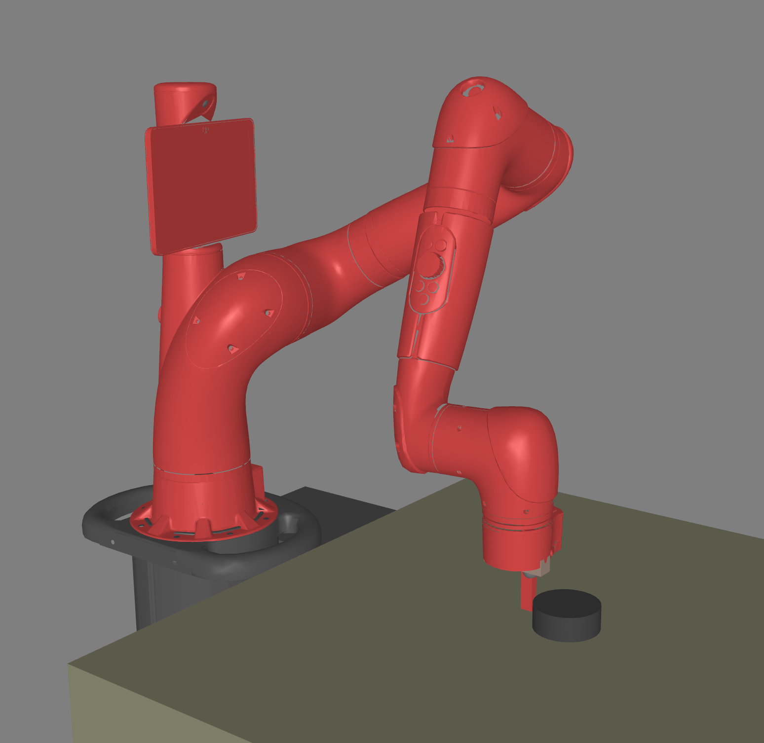
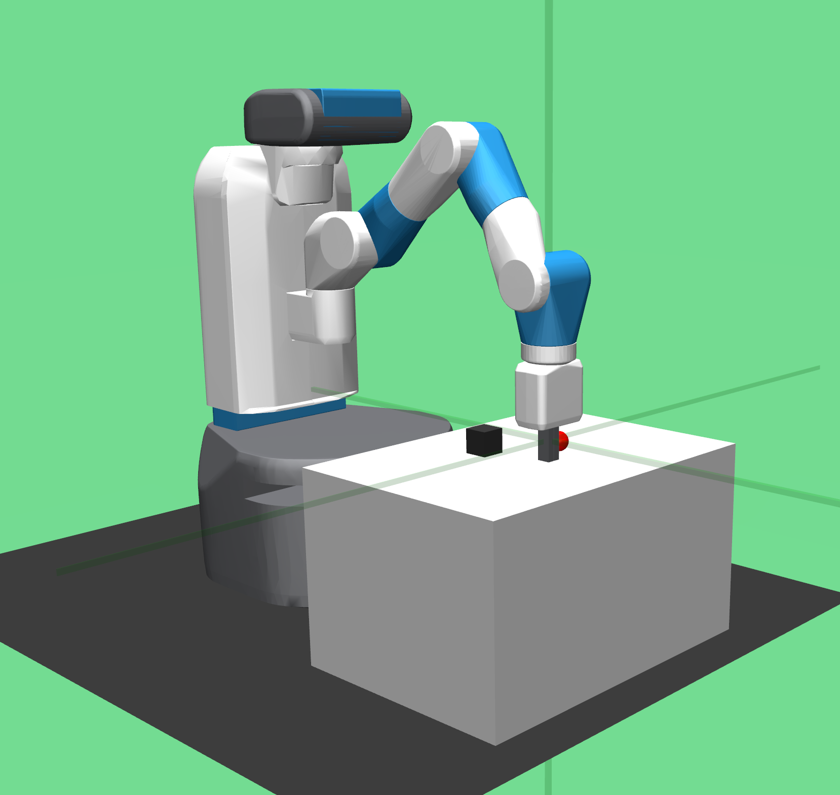
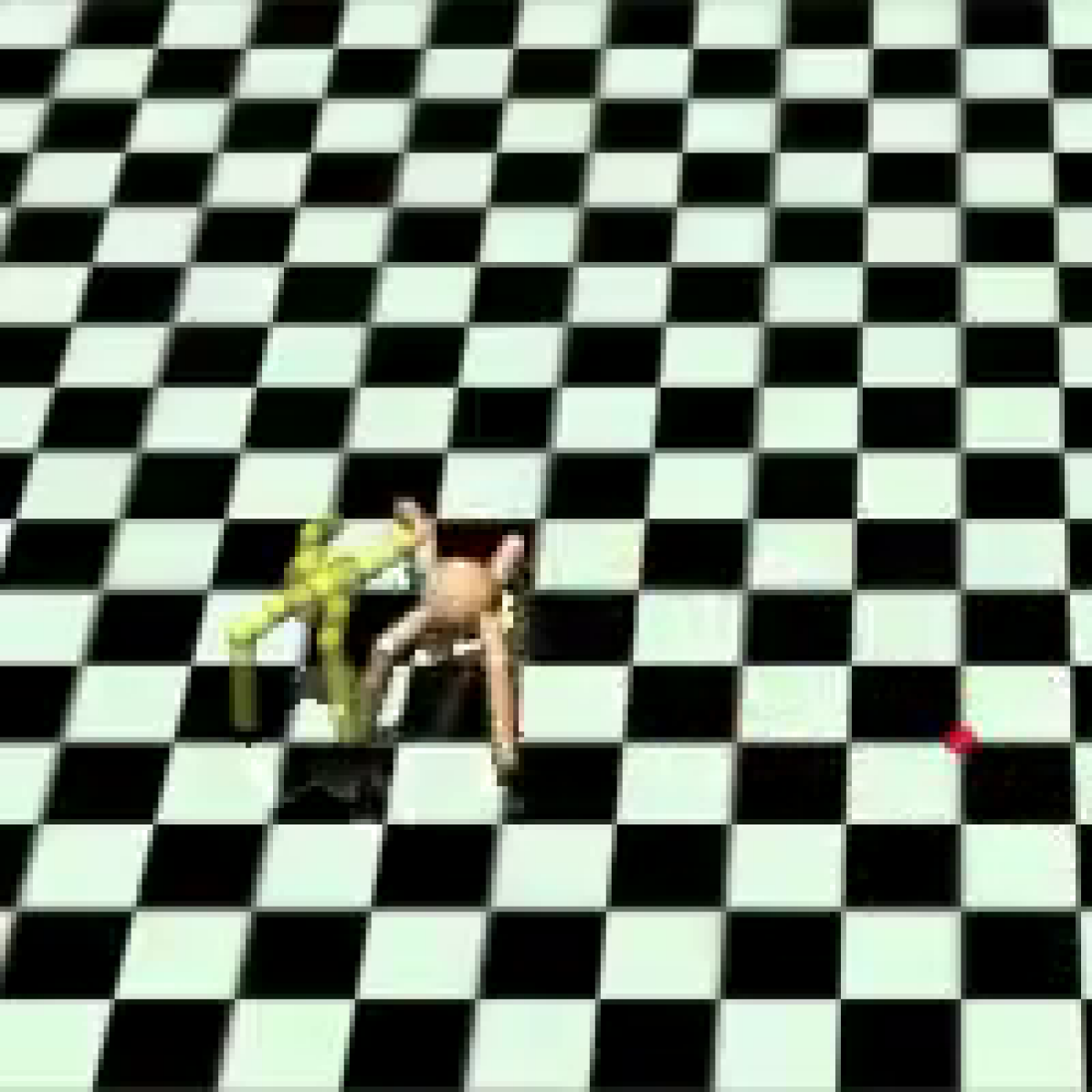
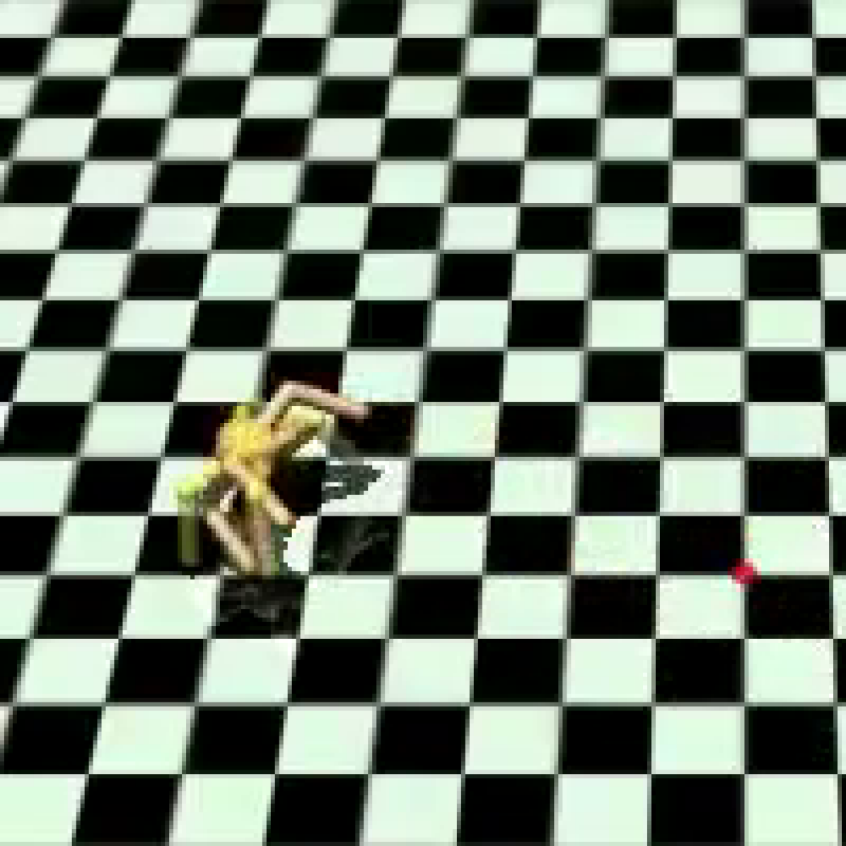
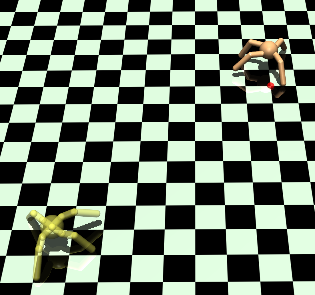
Figure 3: From left to right, we evaluate on: a 2D environment in which an agent must move around a box, a locomotion task in which a quadruped robot must match a location and pose (yellow), and four manipulation tasks in which the robot must push objects, rotate faucet valve, or open a window.

6 Empirical Evaluation

Our experiments compare odac to prior methods for learning goal-conditioned policies and evaluate how the components of our variational objective impact the performance of the method. Specifically, we compare odac to prior methods on a wide range of manipulation and locomotion tasks that require achieving a desired outcome. To answer the second question, we conduct several ablation studies and visualize the behavior of qΔt+1(Δt+1=0)subscript𝑞subscriptΔ𝑡1subscriptΔ𝑡10q_{\Delta_{t+1}}(\Delta_{t+1}=0). In our experiments, we use a uniform action prior p(𝐚)𝑝𝐚p(\mathbf{a}) and the time prior pTsubscript𝑝𝑇p_{T} is geometric with parameter 0.010.010.01, that is, pΔt+1(Δt+1=0)=0.99subscript𝑝subscriptΔ𝑡1subscriptΔ𝑡100.99p_{\Delta_{t+1}}(\Delta_{t+1}=0)=0.99. We begin by describing prior methods and environments used for the experiments.

6.1 Learning to Achieve Desired Outcomes

To avoid over-fitting to any one setting, we compare to these methods across several different robot morphologies and tasks, all illustrated in Figure 3 of the appendix.

Environments.

We compare odac to prior work on a simple 2D navigation task, in which an agent must take non-greedy actions to move around a box, as well as the Ant, Sawyer Push, and Fetch Push simulated robot domains, which have each been studied in prior work on reinforcement learning for reaching goals [2, 28, 30, 34, 41]. For the Ant and Sawyer tasks, desired outcomes correspond to full states (that is, desired positions and joints). For the Fetch task, we use the same goal representation as in prior work [2] and only represent 𝐠𝐠\mathbf{g} with the position of the object. Lastly, we demonstrate the feasibility of replacing manually designed rewards with our outcome-driven paradigm by evaluating the methods on the Sawyer Window and Sawyer Faucet tasks from the MetaWorld benchmark [56]. These tasks come with manually designed reward functions, which we replace by simply specify a desired outcome 𝐠𝐠\mathbf{g}. We plot the mean and standard deviation of the final Euclidean distance to the desired outcome across four random seeds. We normalize the distance to be 111 at the start of training. For further details, see Section C.1.

Goal Sampling.

In all tasks, rather than assuming that we are able to perform oracle goal sampling (which can be difficult or even impossible in complex real-world environments), a fixed desired outcome is commanded as the exploration goal in each episode. During training, the goals are relabeled using the future-style relabeling scheme from Andrychowicz et al. [2]. Unlike oracle goal sampling, this approach does not assume knowledge of the set of admissible states in the environment, but is more realistic and presents a more challenging exploration problem. To challenge the methods, we choose the desired goal to be far from the starting state.

Baselines and Prior Work.

We compare our method to hindsight experience replay (HER) [2], a goal-conditioned method, where the learner receives a reward of 11-1 if it is within an ϵitalic-ϵ\epsilon distance from the goal, and 00 otherwise, universal value density estimation (UVD) [41], which also uses sparse rewards as well as a generative model of the future occupancy measure to estimate the Q𝑄Q-values, and DISCERN [51], which learns a reward function by training a discriminator and using a clipped log-likelihood as the reward. Lastly, we include an oracle Soft Actor–Critic (SAC) baseline that uses a manually designed reward. For the MetaWorld tasks, this baseline uses the benchmark reward for each task. For the remaining environments, this baseline uses the Euclidean distance between the agent’s current and the desired outcome for the reward.

Results.

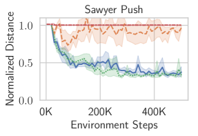
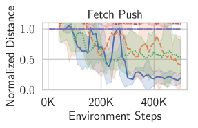
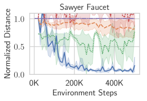
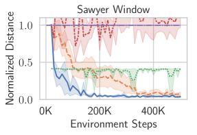
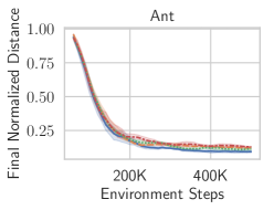
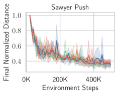
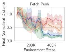
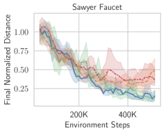
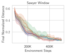
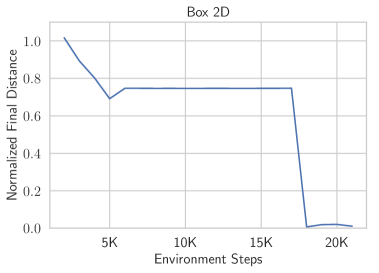
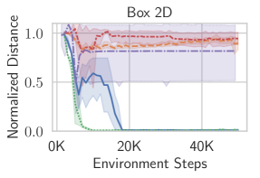
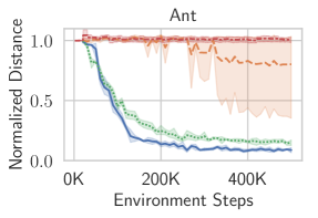
In Figure 4, we see that odac outperforms virtually every method on all tasks, consistently learning faster and often reaching a final distance that is orders of magnitude closer to the desired outcome. The only exception is that the hand-crafted reward learns slightly faster on the 2D task, but this gap is closed within a few ten thousand steps.
Refer to caption
Refer to caption
Refer to caption
Refer to caption
Refer to caption
Refer to caption
Refer to caption
Figure 4: Learning curves showing final distance vs. environment steps across all six environments. Only odac consistently performs well on all six tasks. Prior methods struggle to learn, especially in the absence of uniform goal sampling. See text for details.

6.2 Ablation Study on the Effect of a Variational Discount Factor

Table 1: Ablation results, showing mean final normalized distance (×100absent100\times 100) at the end of training across 4 seeds. Best mean is in bold and standard error in parentheses. odac is not sensitive to the dynamics models p^dsubscript^𝑝𝑑\hat{p}_{d} but benefits from the dynamic qTsubscript𝑞𝑇q_{T} variant.
Env odac fixed p^dsubscript^𝑝𝑑\hat{p}_{d} fixed qTsubscript𝑞𝑇q_{T} fixed qTsubscript𝑞𝑇q_{T}, p^dsubscript^𝑝𝑑\hat{p}_{d}
2D 1.7 (1.20) 1.2 (0.14) 1.0 (0.24) 1.3 (0.29)
Ant 9 (0.48) 11 (0.57) 12 (0.41) 13 (0.20)
Push 35 (2.7) 34 (1.5) 37 (1.5) 38 (3.1)
Fetch 19 (6) 15 (3) 53 (13) 66 (15)
Window 5.4 (0.62) 5.0 (0.62) 7.9 (0.71) 6.0 (0.12)
Faucet 13 (4.2) 15 (3.3) 37 (8.3) 38 (7.2)

Next, we study the importance of the dynamic discount factor qΔt+1(Δt+1=0)subscript𝑞subscriptΔ𝑡1subscriptΔ𝑡10q_{\Delta_{t+1}}(\Delta_{t+1}=0) and the sensitivity of our method to the dynamics model. On all tasks, we evaluate the performance when the posterior exactly matches the prior, that is, qΔt+1(Δt+1=0)=0.99subscript𝑞subscriptΔ𝑡1subscriptΔ𝑡100.99q_{\Delta_{t+1}}(\Delta_{t+1}=0)=0.99 (labeled “fixed qTsubscript𝑞𝑇q_{T}” in Table 1). Our analysis in Section A.3 suggests that this setting is sub-optimal, and this ablation empirically evaluate its benefits. We also measure how the algorithm’s performance depends on the accuracy of the learned dynamics model used for the reward in odac. To do this, we evaluate odac with the dynamics model fixed to a multivariate Laplace distribution with a fixed variance, centered at the previous state (labeled “fixed p^dsubscript^𝑝𝑑\hat{p}_{d}” in Table 1). This ablation represents an extremely crude model, and good performance with such a model would indicate that our method does not depend on obtaining an particularly accurate model.

In Table 1, we see that fixing the distribution qTsubscript𝑞𝑇q_{T} to the prior pTsubscript𝑝𝑇p_{T} as described in Corollary 3 deteriorates performance, and that using a learned or fixed model both perform relatively well. These results suggest that the derived optimal variational distribution qΔt+1(Δt+1=0)superscriptsubscript𝑞subscriptΔ𝑡1subscriptΔ𝑡10q_{\Delta_{t+1}}^{\star}(\Delta_{t+1}=0) given in Proposition 2 is better not only in theory but also in practice, and that odac is not sensitive to the accuracy of the dynamics model. Moreover, we note that a more expressive dynamics model—which could lead to a tighter variational bound—may not necessarily lead to a better variational policy if the functional form of the log-density under the dynamics model does not also provide favorable shaping.

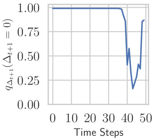
In Appendix B, we provide the full learning curves for this ablation study and present further experiments. For example, we compare odac to a variant in which we use the learned dynamics model for model-based planning. We find that using the dynamics model only to compute rewards significantly outperforms the variant where it is used for both computing rewards and model-based planning. This result suggests that odac does not require learning a dynamics model that is accurate enough for planning, and that the derived Bellman updates are sufficient for obtaining policies that can achieve desired outcomes. In Figure 7, we also visualize qTsubscript𝑞𝑇q_{T} and find that as the policy reaches an irrecoverable state, qΔt+1(Δt+1=0)subscript𝑞subscriptΔ𝑡1subscriptΔ𝑡10q_{\Delta_{t+1}}(\Delta_{t+1}=0) drops in value, suggesting that odac automatically learns a dynamic discount factor that terminates an episode when an irrecoverable state is reached.

7 Conclusion

We proposed a probabilistic approach for achieving desired outcomes in settings where no reward function and no termination condition are given. We showed that by framing the problem of achieving desired outcomes as variational inference, we can derive an off-policy temporal-difference algorithm, a reward function learnable from environment interactions, and a novel Bellman backup that contains a state–action dependent dynamic discount factor for the reward and bootstrap term.

Our experimental results demonstrated that the resulting algorithm, odac, leads to efficient outcome-driven approaches to RL. While odac requires choosing a dynamics model, we found that it works well even for simple dynamics models and believe that the use of more sophisticated dynamics models that incorporate epistemic uncertainty [7] or domain-specific structure [8, 38, 49, 57] is a promising avenue for future research.

Acknowledgments and Disclosure of Funding

We thank Marvin Zhang, Michael Janner, Abhishek Gupta, and various RAIL and OATML students for their discussions and feedback on early drafts of this paper. Tim G. J. Rudner is funded by the Rhodes Trust, by a Qualcomm Innovation Fellowship, and by the Engineering and Physical Sciences Research Council (EPSRC). This research was further supported by the Alan Turing Institute, the National Science Foundation, the DARPA Assured Autonomy Program, and ARL DCIST CRA W911NF-17-2-0181.

References

  • Aly and Chan [1974] G.M Aly and W.C Chan. Numerical computation of optimal control problems with unknown final time. Journal of Mathematical Analysis and Applications, 45(2):274–284, 1974. ISSN 0022-247X.
  • Andrychowicz et al. [2017] Marcin Andrychowicz, Filip Wolski, Alex Ray, Jonas Schneider, Rachel Fong, Peter Welinder, Bob Mcgrew, Josh Tobin, Pieter Abbeel, and Wojciech Zaremba. Hindsight experience replay. In Neural Information Processing Systems (NeurIPS), 2017.
  • Attias [2003] H. Attias. Planning by probabilistic inference. In Proceedings of the 9th International Workshop on Artificial Intelligence and Statistics, 2003.
  • Brockman et al. [2016] Greg Brockman, Vicki Cheung, Ludwig Pettersson, Jonas Schneider, John Schulman, Jie Tang, and Wojciech Zaremba. Openai gym. arXiv preprint arXiv:1606.01540, 2016.
  • Chen et al. [2018] Yongxin Chen, Tryphon T. Georgiou, and Michele Pavon. Optimal steering of a linear stochastic system to a final probability distribution—part iii. IEEE Transactions on Automatic Control, 63(9):3112–3118, 2018.
  • Choi et al. [2021] Jongwook Choi, Archit Sharma, Honglak Lee, Sergey Levine, and Shixiang Shane Gu. Variational empowerment as representation learning for goal-based reinforcement learning. In International Conference on Machine Learning (ICML), 2021.
  • Chua et al. [2018] Kurtland Chua, Roberto Calandra, Rowan Mcallister, and Sergey Levine. Deep reinforcement learning in a handful of trials using probabilistic dynamics models. In Advances in Neural Information Processing Systems, 2018.
  • Ebert et al. [2017] Frederik Ebert, Chelsea Finn, Alex X Lee, and Sergey Levine. Self-supervised visual planning with temporal skip connections. In Conference on Robot Learning (CoRL), 2017.
  • Eysenbach et al. [2019] Benjamin Eysenbach, Ruslan Salakhutdinov, and Sergey Levine. Search on the replay buffer: Bridging planning and reinforcement learning. arXiv preprint arXiv:1906.05253, 2019.
  • Fellows et al. [2019] Matthew Fellows, Anuj Mahajan, Tim G. J. Rudner, and Shimon Whiteson. VIREL: A variational inference framework for reinforcement learning. In Advances in Neural Information Processing Systems 32, 2019.
  • Fu et al. [2018] Justin Fu, Avi Singh, Dibya Ghosh, Larry Yang, and Sergey Levine. Variational inverse control with events: A general framework for data-driven reward definition. In S. Bengio, H. Wallach, H. Larochelle, K. Grauman, N. Cesa-Bianchi, and R. Garnett, editors, Neural Information Processing Systems (NeurIPS), pages 8538–8547. 2018.
  • Fujimoto et al. [2018] Scott Fujimoto, Herke van Hoof, and David Meger. Addressing function approximation error in actor-critic methods. International Conference on Machine Learning (ICML), 2018.
  • Galashov et al. [2019] Alexandre Galashov, Siddhant M. Jayakumar, Leonard Hasenclever, Dhruva Tirumala, Jonathan Schwarz, Guillaume Desjardins, Wojciech M. Czarnecki, Yee Whye Teh, Razvan Pascanu, and Nicolas Heess. Information asymmetry in KL-regularized RL. In 7th International Conference on Learning Representations, ICLR 2019, New Orleans, LA, USA, May 6-9, 2019, 2019.
  • Goebel and Raitums [1990] Manfred Goebel and Uldis Raitums. Optimal control of two point boundary value problems. In H. J. Sebastian and K. Tammer, editors, System Modelling and Optimization, pages 281–290, Berlin, Heidelberg, 1990. Springer Berlin Heidelberg.
  • Grigoriadis and Skelton [1997] Karolos M. Grigoriadis and Robert E. Skelton. Minimum-energy covariance controllers. Automatica, 33(4):569–578, 1997. ISSN 0005-1098.
  • Haarnoja et al. [2018a] Tuomas Haarnoja, Aurick Zhou, Pieter Abbeel, and Sergey Levine. Soft actor-critic: Off-policy maximum entropy deep reinforcement learning with a stochastic actor. In International Conference on Machine Learning, 2018a.
  • Haarnoja et al. [2018b] Tuomas Haarnoja, Aurick Zhou, Kristian Hartikainen, George Tucker, Sehoon Ha, Jie Tan, Vikash Kumar, Henry Zhu, Abhishek Gupta, Pieter Abbeel, and Sergey Levine. Soft actor-critic algorithms and applications, 2018b.
  • Hartikainen et al. [2020] Kristian Hartikainen, Xinyang Geng, Tuomas Haarnoja, and Sergey Levine. Dynamical distance learning for unsupervised and semi-supervised skill discovery. In International Conference on Learning Representations (ICLR), 2020.
  • Hoffman et al. [2009] Matthew Hoffman, Nando Freitas, Arnaud Doucet, and Jan Peters. An expectation maximization algorithm for continuous markov decision processes with arbitrary reward. In Artificial intelligence and statistics, pages 232–239, 2009.
  • Hotz and Skelton [1987] Anthony F. Hotz and Robert E. Skelton. A covariance control theory. In System Identification and Adaptive Control, Part 2 of 3, volume 26 of Control and Dynamic Systems, pages 225–276. Academic Press, 1987.
  • Janner et al. [2019] Michael Janner, Justin Fu, Marvin Zhang, and Sergey Levine. When to trust your model: Model-based policy optimization. In Advances in Neural Information Processing Systems, 2019.
  • Kaelbling [1993] Leslie P Kaelbling. Learning to achieve goals. In International Joint Conference on Artificial Intelligence (IJCAI), volume vol.2, pages 1094 – 8, 1993.
  • Kappen et al. [2012] H. J. Kappen, V. Gómez, and M. Opper. Optimal control as a graphical model inference problem. Machine Learning, 87(2):159–182, 2012.
  • Kárnỳ [1996] Miroslav Kárnỳ. Towards fully probabilistic control design. Automatica, 32(12):1719–1722, 1996.
  • Levine [2018] Sergey Levine. Reinforcement learning and control as probabilistic inference: Tutorial and review. 2018.
  • Levy et al. [2017] Andrew Levy, George Konidaris, Robert Platt, and Kate Saenko. Learning multi-level hierarchies with hindsight. arXiv preprint arXiv:1712.00948, 2017.
  • Lillicrap et al. [2016] Timothy P Lillicrap, Jonathan J Hunt, Alexander Pritzel, Nicolas Heess, Tom Erez, Yuval Tassa, David Silver, and Daan Wierstra. Continuous control with deep reinforcement learning. In International Conference on Learning Representations (ICLR), 2016.
  • Nachum et al. [2018] Ofir Nachum, Google Brain, Shixiang Gu, Honglak Lee, and Sergey Levine. Data-efficient hierarchical reinforcement learning. In Neural Information Processing Systems (NeurIPS), 2018.
  • Nagabandi et al. [2018] Anusha Nagabandi, Gregory Kahn, Ronald S Fearing, and Sergey Levine. Neural network dynamics for model-based deep reinforcement learning with model-free fine-tuning. In IEEE International Conference on Robotics and Automation (ICRA), 2018.
  • Nair et al. [2018] Ashvin Nair, Vitchyr Pong, Murtaza Dalal, Shikhar Bahl, Steven Lin, and Sergey Levine. Visual reinforcement learning with imagined goals. In Neural Information Processing Systems (NeurIPS), 2018.
  • Peters et al. [2010] Jan Peters, Katharina Mülling, and Yasemin Altün. Relative entropy policy search. In AAAI Conference on Artificial Intelligence, pages 1607–1612, 2010.
  • Plappert et al. [2018] Matthias Plappert, Marcin Andrychowicz, Alex Ray, Bob Mcgrew, Bowen Baker, Glenn Powell, Jonas Schneider, Josh Tobin, Maciek Chociej, Peter Welinder, Vikash Kumar, and Wojciech Zaremba. Multi-goal reinforcement learning: Challenging robotics environments and request for research. arXiv preprint arXiv:1802.09464, 2018.
  • Pong et al. [2018] Vitchyr Pong, Shixiang Gu, Murtaza Dalal, and Sergey Levine. Temporal difference models: Model-free deep RL for model-based control. In International Conference on Learning Representations (ICLR), 2018.
  • Pong et al. [2019] Vitchyr H. Pong, Murtaza Dalal, Steven Lin, Ashvin Nair, Shikhar Bahl, and Sergey Levine. Skew-Fit: State-covering self-supervised reinforcement learning. arXiv preprint arXiv:1903.03698, abs/1903.03698, 2019.
  • Rawlik et al. [2013] K. Rawlik, M. Toussaint, and S. Vijayakumar. On stochastic optimal control and reinforcement learning by approximate inference. In Robotics: Science and Systems (RSS), 2013.
  • Rawlik et al. [2010] Konrad Rawlik, Marc Toussaint, and Sethu Vijayakumar. An approximate inference approach to temporal optimization in optimal control. In J. Lafferty, C. Williams, J. Shawe-Taylor, R. Zemel, and A. Culotta, editors, Advances in Neural Information Processing Systems, volume 23. Curran Associates, Inc., 2010.
  • Ridderhof et al. [2019] Jack Ridderhof, Kazuhide Okamoto, and Panagiotis Tsiotras. Nonlinear uncertainty control with iterative covariance steering, 2019.
  • Rudner et al. [2021a] Tim G. J. Rudner, Zonghao Chen, and Yarin Gal. Rethinking function-space variational inference in Bayesian neural networks. In Third Symposium on Advances in Approximate Bayesian Inference, 2021a.
  • Rudner et al. [2021b] Tim G. J. Rudner, Cong Lu, Michael A. Osborne, Yarin Gal, and Yee Whye Teh. On pathologies in KL-regularized reinforcement learning from expert demonstrations. In Advances in Neural Information Processing Systems 34. 2021b.
  • Schaul et al. [2015] Tom Schaul, Daniel Horgan, Karol Gregor, and David Silver. Universal value function approximators. In International Conference on Machine Learning (ICML), pages 1312–1320, 2015.
  • Schroecker and Isbell [2020] Yannick Schroecker and Charles Isbell. Universal value density estimation for imitation learning and goal-conditioned reinforcement learning. arXiv preprint arXiv:2002.06473, 2020.
  • Singh et al. [2019] Avi Singh, Larry Yang, Kristian Hartikainen, Chelsea Finn, and Sergey Levine. End-to-end robotic reinforcement learning without reward engineering. arXiv preprint arXiv:1904.07854, 2019.
  • Sutton and Barto [1998] Richard S Sutton and Andrew G Barto. Reinforcement Learning: An Introduction. 1998.
  • Szepesvári [2010] Csaba Szepesvári. Algorithms for Reinforcement Learning, volume 4. 2010.
  • Todorov [2006] E. Todorov. Linearly-solvable Markov decision problems. In Neural Information Processing Systems (NeurIPS), 2006.
  • Toussaint [2009] M. Toussaint. Robot trajectory optimization using approximate inference. In International Conference on Machine Learning (ICML), 2009.
  • Toussaint and Storkey [2006] Marc Toussaint and Amos Storkey. Probabilistic inference for solving discrete and continuous state Markov decision processes. In Proceedings of the 23rd international conference on Machine learning, pages 945–952, 2006.
  • Toussaint et al. [2006] Marc Toussaint, Stefan Harmeling, and Amos Storkey. Probabilistic inference for solving (PO)MDPs. Technical report, 2006.
  • Veerapaneni et al. [2020] Rishi Veerapaneni, John D Co-Reyes, Michael Chang, Michael Janner, Chelsea Finn, Jiajun Wu, Joshua Tenenbaum, and Sergey Levine. Entity abstraction in visual model-based reinforcement learning. In Conference on Robot Learning, pages 1439–1456. PMLR, 2020.
  • Venkattaramanujam et al. [2019] Srinivas Venkattaramanujam, Eric Crawford, Thang Doan, and Doina Precup. Self-supervised learning of distance functions for goal-conditioned reinforcement learning. arXiv:1907.02998, 2019.
  • Warde-Farley et al. [2019] David Warde-Farley, Tom Van De Wiele, Tejas Kulkarni, Catalin Ionescu, Steven Hansen, & Volodymyr, and Mnih Deepmind. Unsupervised control through non-parametric discriminative rewards. In International Conference on Learning Representations (ICLR), 2019.
  • Watkins and Dayan [1992] Christopher JCH Watkins and Peter Dayan. Q-learning. Machine learning, 8(3-4):279–292, 1992.
  • White [2017] Martha White. Unifying task specification in reinforcement learning. In International Conference on Machine Learning, pages 3742–3750. PMLR, 2017.
  • Xu and Skelton [1992] J.-H. Xu and R.E. Skelton. An improved covariance assignment theory for discrete systems, 1992.
  • Yi et al. [2020] Z. Yi, Z. Cao, E. Theodorou, and Y. Chen. Nonlinear covariance control via differential dynamic programming. In 2020 American Control Conference (ACC), pages 3571–3576, 2020.
  • Yu et al. [2020] Tianhe Yu, Deirdre Quillen, Zhanpeng He, Ryan Julian, Karol Hausman, Chelsea Finn, and Sergey Levine. Meta-world: A benchmark and evaluation for multi-task and meta reinforcement learning. In Conference on Robot Learning, pages 1094–1100. PMLR, 2020.
  • Zhang et al. [2019] Marvin Zhang, Sharad Vikram, Laura Smith, Pieter Abbeel, Matthew J. Johnson, and Sergey Levine. SOLAR: Deep structured representations for model-based reinforcement learning. In International Conference on Machine Learning (ICML), aug 2019.
  • Ziebart et al. [2008] Brian D Ziebart, Andrew Maas, J Andrew Bagnell, and Anind K Dey. Maximum entropy inverse reinforcement learning. In AAAI Conference on Artificial Intelligence, pages 1433–1438, 2008.

Supplementary Material

Table of Contents

Appendix A Proofs & Derivations

A.1 Finite- and Infinite-Horizon Variational Objectives

In this section, we present detailed derivations and proofs for the results in Sections 3.1 and Section 3.2.

Proposition 1 (Fixed-Time Outcome-Driven Variational Objective).

Let q𝓣~0:t|𝐒0(𝛕~0:t|𝐬0)subscript𝑞conditionalsubscript~𝓣:0𝑡subscript𝐒0conditionalsubscript~𝛕:0𝑡subscript𝐬0q_{\tilde{\bm{\mathcal{T}}}_{0:t}|\mathbf{S}_{0}}(\tilde{\bm{\tau}}_{0:t}\,|\,\mathbf{s}_{0}) be as defined in Equation 3. Then, given any initial state 𝐬0subscript𝐬0\mathbf{s}_{0}, termination time tsuperscript𝑡t^{\star}, and outcome 𝐠𝐠\mathbf{g},

𝔻KL(q𝓣~0:t|𝐒0(|𝐬0)p𝓣~0:t|𝐒0,𝐒t(|𝐬0,𝐠))=logp(𝐠|𝐬0)¯(π,𝐬0,𝐠),\displaystyle\begin{split}\mathbb{D}_{\emph{{KL}}}(q_{\tilde{\bm{\mathcal{T}}}_{0:t}|\mathbf{S}_{0}}(\cdot\,|\,\mathbf{s}_{0})\,\|\,p_{\tilde{\bm{\mathcal{T}}}_{0:t}|\mathbf{S}_{0},\mathbf{S}_{t^{\star}}}(\cdot\,|\,\mathbf{s}_{0},\mathbf{g}))=\log p(\mathbf{g}\,|\,\mathbf{s}_{0})-\bar{\mathcal{F}}(\pi,\mathbf{s}_{0},\mathbf{g}),\end{split} (A.1)

where

¯(π,𝐬0,𝐠)=˙𝔼q𝓣~0:t|𝐒0(𝝉~0:t|𝐬0)[logpd(𝐠|𝐬t,𝐚t)t=0t1𝔻KL(π(|𝐬t)||p(|𝐬t))],\displaystyle\begin{split}\SwapAboveDisplaySkip\bar{\mathcal{F}}(\pi,\mathbf{s}_{0},\mathbf{g})\,\,\dot{=}\,\,\mathbb{E}_{q_{\tilde{\bm{\mathcal{T}}}_{0:t}|\mathbf{S}_{0}}(\tilde{\bm{\tau}}_{0:t}\,|\,\mathbf{s}_{0})}\bigg{[}&\log p_{d}(\mathbf{g}\,|\,\mathbf{s}_{t},\mathbf{a}_{t})-\sum_{t^{\prime}=0}^{t-1}\mathbb{D}_{\emph{{KL}}}(\pi(\cdot\,|\,\mathbf{s}_{t^{\prime}})\,||\,p(\cdot\,|\,\mathbf{s}_{t^{\prime}}))\bigg{]},\end{split} (A.2)

and since logp(𝐠|𝐬0)𝑝conditional𝐠subscript𝐬0\log p(\mathbf{g}|\mathbf{s}_{0}) is constant in π𝜋\pi,

argminπΠ𝔻KL(q𝓣~0:t|𝐒0(|𝐬0)p𝓣~0:t|𝐒0,𝐒t(|𝐬0,𝐠))=argmaxπΠ¯(π,𝐬0,𝐠).\displaystyle\operatorname*{arg\,min}_{\pi\in\Pi}\mathbb{D}_{\emph{{KL}}}(q_{\tilde{\bm{\mathcal{T}}}_{0:t}|\mathbf{S}_{0}}(\cdot\,|\,\mathbf{s}_{0})\,\|\,p_{\tilde{\bm{\mathcal{T}}}_{0:t}|\mathbf{S}_{0},\mathbf{S}_{t^{\star}}}(\cdot\,|\,\mathbf{s}_{0},\mathbf{g}))=\operatorname*{arg\,max}_{\pi\in\Pi}\bar{\mathcal{F}}(\pi,\mathbf{s}_{0},\mathbf{g}). (A.3)
Proof.

To find an approximation to the posterior p𝓣~0:t|𝐒0,𝐒t(|𝐬0,𝐠)p_{\tilde{\bm{\mathcal{T}}}_{0:t}|\mathbf{S}_{0},\mathbf{S}_{t^{\star}}}(\cdot\,|\,\mathbf{s}_{0},\mathbf{g}), we can use variational inference. To do so, we consider the trajectory distribution under p𝓣~0:t|𝐒0,𝐒t(|𝐬0,𝐠)p_{\tilde{\bm{\mathcal{T}}}_{0:t}|\mathbf{S}_{0},\mathbf{S}_{t^{\star}}}(\cdot\,|\,\mathbf{s}_{0},\mathbf{g}), which by Bayes’ Theorem is given by

p𝓣~0:t|𝐒0,𝐒t(𝝉~0:t|𝐬0,𝐠)=pd(𝐠|𝐬t,𝐚t)p(𝐚t|𝐬t)t=0t1pd(𝐬t+1|𝐬t,𝐚t)p(𝐚t|𝐬t)p(𝐠|𝐬0),subscript𝑝conditionalsubscript~𝓣:0𝑡subscript𝐒0subscript𝐒superscript𝑡conditionalsubscript~𝝉:0𝑡subscript𝐬0𝐠subscript𝑝𝑑conditional𝐠subscript𝐬𝑡subscript𝐚𝑡𝑝conditionalsubscript𝐚𝑡subscript𝐬𝑡superscriptsubscriptproductsuperscript𝑡0𝑡1subscript𝑝𝑑conditionalsubscript𝐬superscript𝑡1subscript𝐬𝑡subscript𝐚𝑡𝑝conditionalsubscript𝐚superscript𝑡subscript𝐬superscript𝑡𝑝conditional𝐠subscript𝐬0\displaystyle p_{\tilde{\bm{\mathcal{T}}}_{0:t}|\mathbf{S}_{0},\mathbf{S}_{t^{\star}}}(\tilde{\bm{\tau}}_{0:t}\,|\,\mathbf{s}_{0},\mathbf{g})=\frac{p_{d}(\mathbf{g}\,|\,\mathbf{s}_{t},\mathbf{a}_{t})p(\mathbf{a}_{t}\,|\,\mathbf{s}_{t})\prod_{t^{\prime}=0}^{t-1}p_{d}(\mathbf{s}_{t^{\prime}+1}\,|\,\mathbf{s}_{t},\mathbf{a}_{t})p(\mathbf{a}_{t^{\prime}}\,|\,\mathbf{s}_{t^{\prime}})}{p(\mathbf{g}\,|\,\mathbf{s}_{0})}, (A.4)

where t=t1𝑡superscript𝑡1t=t^{\star}-1, and we denote the state–action trajectory realization from action 𝐚0subscript𝐚0\mathbf{a}_{0} to 𝐚tsubscript𝐚𝑡\mathbf{a}_{t} by 𝝉~0:t=˙{𝐚0,𝐬1,𝐚1,,𝐬t,𝐚t}subscript~𝝉:0𝑡˙subscript𝐚0subscript𝐬1subscript𝐚1subscript𝐬𝑡subscript𝐚𝑡\tilde{\bm{\tau}}_{0:t}\,\,\dot{=}\,\,\{\mathbf{a}_{0},\mathbf{s}_{1},\mathbf{a}_{1},...,\mathbf{s}_{t},\mathbf{a}_{t}\}. Inferring an approximation to the posterior distribution p𝓣~0:t|𝐒0,𝐒t(|𝐬0,𝐠)p_{\tilde{\bm{\mathcal{T}}}_{0:t}|\mathbf{S}_{0},\mathbf{S}_{t^{\star}}}(\cdot\,|\,\mathbf{s}_{0},\mathbf{g}) then becomes equivalent to finding a variational distribution q𝓣~0:T|𝐒0(|𝐬0)q_{\tilde{\bm{\mathcal{T}}}_{0:T}|\mathbf{S}_{0}}(\cdot\,|\,\mathbf{s}_{0}), which induces a trajectory distribution q𝓣~0:t|𝐒0(|𝐬0)q_{\tilde{\bm{\mathcal{T}}}_{0:t}|\mathbf{S}_{0}}(\cdot\,|\,\mathbf{s}_{0}) that minimizes the KL divergence from q𝓣~0:t|𝐒0(|𝐬0)q_{\tilde{\bm{\mathcal{T}}}_{0:t}|\mathbf{S}_{0}}(\cdot\,|\,\mathbf{s}_{0}) to p𝓣~0:t|𝐒0,𝐒t(|𝐬0,𝐠)p_{\tilde{\bm{\mathcal{T}}}_{0:t}|\mathbf{S}_{0},\mathbf{S}_{t^{\star}}}(\cdot\,|\,\mathbf{s}_{0},\mathbf{g}):

minq𝒬¯𝔻KL(q𝓣~0:t|𝐒0(|𝐬0)p𝓣~0:t|𝐒0,𝐒t(|𝐬0,𝐠)).\displaystyle\min_{q\in\bar{\mathcal{Q}}}\mathbb{D}_{\text{KL}}(q_{\tilde{\bm{\mathcal{T}}}_{0:t}|\mathbf{S}_{0}}(\cdot\,|\,\mathbf{s}_{0})\;\|\;p_{\tilde{\bm{\mathcal{T}}}_{0:t}|\mathbf{S}_{0},\mathbf{S}_{t^{\star}}}(\cdot\,|\,\mathbf{s}_{0},\mathbf{g})). (A.5)

If we find a distribution q𝓣~0:t|𝐒0(|𝐬0)q_{\tilde{\bm{\mathcal{T}}}_{0:t}|\mathbf{S}_{0}}(\cdot\,|\,\mathbf{s}_{0}) for which the resulting KL divergence is zero, then q𝓣~0:t|𝐒0(|𝐬0)q_{\tilde{\bm{\mathcal{T}}}_{0:t}|\mathbf{S}_{0}}(\cdot\,|\,\mathbf{s}_{0}) is the exact posterior. If the KL divergence is positive, then q𝓣~0:t|𝐒0(|𝐬0)q_{\tilde{\bm{\mathcal{T}}}_{0:t}|\mathbf{S}_{0}}(\cdot\,|\,\mathbf{s}_{0}) is an approximate posterior. To solve the variational problem in Equation A.5, we can define a factorized variational family

q𝓣~0:t|𝐒0(𝝉~0:t|𝐬0)=˙π(𝐚t|𝐬t)t=0t1q𝐒t+1|𝐒t,𝐀t(𝐬t+1|𝐬t,𝐚t)π(𝐚t|𝐬t),subscript𝑞conditionalsubscript~𝓣:0𝑡subscript𝐒0conditionalsubscript~𝝉:0𝑡subscript𝐬0˙𝜋conditionalsubscript𝐚𝑡subscript𝐬𝑡superscriptsubscriptproductsuperscript𝑡0𝑡1subscript𝑞conditionalsubscript𝐒superscript𝑡1subscript𝐒superscript𝑡subscript𝐀superscript𝑡conditionalsubscript𝐬superscript𝑡1subscript𝐬superscript𝑡subscript𝐚superscript𝑡𝜋conditionalsubscript𝐚superscript𝑡subscript𝐬superscript𝑡\displaystyle q_{\tilde{\bm{\mathcal{T}}}_{0:t}|\mathbf{S}_{0}}(\tilde{\bm{\tau}}_{0:t}\,|\,\mathbf{s}_{0})\,\,\dot{=}\,\,\pi(\mathbf{a}_{t}\,|\,\mathbf{s}_{t})\prod_{t^{\prime}=0}^{t-1}q_{\mathbf{S}_{t^{\prime}+1}|\mathbf{S}_{t^{\prime}},\mathbf{A}_{t^{\prime}}}(\mathbf{s}_{t^{\prime}+1}\,|\,\mathbf{s}_{t^{\prime}},\mathbf{a}_{t^{\prime}})\pi(\mathbf{a}_{t^{\prime}}\,|\,\mathbf{s}_{t^{\prime}}), (A.6)

where 𝐀0:tsubscript𝐀:0𝑡\mathbf{A}_{0:t} and 𝐒1:tsubscript𝐒:1𝑡\mathbf{S}_{1:t} are latent variables over which to infer an approximate posterior distribution, and the product is from t=0𝑡0t=0 to t=t1𝑡superscript𝑡1t=t^{\star}-1 to exclude the conditional distribution over the (observed) state 𝐒t+1=𝐠subscript𝐒𝑡1𝐠\mathbf{S}_{t+1}=\mathbf{g} from the variational distribution.

Returning to the variational problem in Equation A.5, we can now write

𝔻KL(q𝓣~0:t|𝐒0(|𝐬0)p𝓣~0:t|𝐒0,𝐒t(|𝐬0,𝐠))=𝒜t+1𝒮tq𝓣~0:t|𝐒0(𝝉~0:t|𝐬0)logq𝓣~0:t|𝐒0(𝝉~0:t|𝐬0)p𝓣~0:t|𝐒0,𝐒t(𝝉~0:t|𝐬0,𝐠)d𝐬1:td𝐚0:t=¯(π,𝐬0,𝐠)+logp(𝐠|𝐬0),\displaystyle\begin{split}&\mathbb{D}_{\text{KL}}(q_{\tilde{\bm{\mathcal{T}}}_{0:t}|\mathbf{S}_{0}}(\cdot\,|\,\mathbf{s}_{0})\;\|\;p_{\tilde{\bm{\mathcal{T}}}_{0:t}|\mathbf{S}_{0},\mathbf{S}_{t^{\star}}}(\cdot\,|\,\mathbf{s}_{0},\mathbf{g}))\\ &=\int_{\mathcal{A}^{t+1}}\int_{\mathcal{S}^{t}}q_{\tilde{\bm{\mathcal{T}}}_{0:t}|\mathbf{S}_{0}}(\tilde{\bm{\tau}}_{0:t}\,|\,\mathbf{s}_{0})\log\frac{q_{\tilde{\bm{\mathcal{T}}}_{0:t}|\mathbf{S}_{0}}(\tilde{\bm{\tau}}_{0:t}\,|\,\mathbf{s}_{0})}{p_{\tilde{\bm{\mathcal{T}}}_{0:t}|\mathbf{S}_{0},\mathbf{S}_{t^{\star}}}(\tilde{\bm{\tau}}_{0:t}|\mathbf{s}_{0},\mathbf{g})}d\mathbf{s}_{1:t}d\mathbf{a}_{0:t}\\ &=-\bar{\mathcal{F}}(\pi,\mathbf{s}_{0},\mathbf{g})+\log p(\mathbf{g}|\mathbf{s}_{0}),\end{split} (A.7)

where

¯(π,𝐬0,𝐠)=˙𝔼q𝓣~0:t|𝐒0(𝝉~0:t|𝐬0)[logpd(𝐠|𝐬t,𝐚t)+logp(𝐚t|𝐬t)logπ(𝐚t|𝐬t)+t=0t1logp(𝐚t|𝐬t)+logpd(𝐬t+1|𝐬t,𝐚t)logπ(𝐚t|𝐬t)logq𝐒t+1|𝐒t,𝐀t(𝐬t+1|𝐬t,𝐚t)]¯𝜋subscript𝐬0𝐠˙subscript𝔼subscript𝑞conditionalsubscript~𝓣:0𝑡subscript𝐒0conditionalsubscript~𝝉:0𝑡subscript𝐬0delimited-[]subscript𝑝𝑑|𝐠subscript𝐬𝑡subscript𝐚𝑡𝑝|subscript𝐚𝑡subscript𝐬𝑡𝜋|subscript𝐚𝑡subscript𝐬𝑡superscriptsubscriptsuperscript𝑡0𝑡1𝑝|subscript𝐚superscript𝑡subscript𝐬superscript𝑡subscript𝑝𝑑|subscript𝐬superscript𝑡1subscript𝐬superscript𝑡subscript𝐚superscript𝑡𝜋|subscript𝐚superscript𝑡subscript𝐬superscript𝑡subscript𝑞conditionalsubscript𝐒superscript𝑡1subscript𝐒superscript𝑡subscript𝐀superscript𝑡|subscript𝐬superscript𝑡1subscript𝐬superscript𝑡subscript𝐚superscript𝑡\displaystyle\begin{split}&\bar{\mathcal{F}}(\pi,\mathbf{s}_{0},\mathbf{g})\\ &\,\,\dot{=}\,\,\mathbb{E}_{q_{\tilde{\bm{\mathcal{T}}}_{0:t}|\mathbf{S}_{0}}(\tilde{\bm{\tau}}_{0:t}\,|\,\mathbf{s}_{0})}\Bigg{[}\log p_{d}(\mathbf{g}\,|\,\mathbf{s}_{t},\mathbf{a}_{t})+\log p(\mathbf{a}_{t}\,|\,\mathbf{s}_{t})-\log\pi(\mathbf{a}_{t}\,|\,\mathbf{s}_{t})\\ &\qquad\quad+\sum_{t^{\prime}=0}^{t-1}\log p(\mathbf{a}_{t^{\prime}}\,|\,\mathbf{s}_{t^{\prime}})+\log p_{d}(\mathbf{s}_{t^{\prime}+1}\,|\,\mathbf{s}_{t^{\prime}},\mathbf{a}_{t^{\prime}})-\log\pi(\mathbf{a}_{t^{\prime}}\,|\,\mathbf{s}_{t^{\prime}})-\log q_{\mathbf{S}_{t^{\prime}+1}|\mathbf{S}_{t^{\prime}},\mathbf{A}_{t^{\prime}}}(\mathbf{s}_{t^{\prime}+1}\,|\,\mathbf{s}_{t^{\prime}},\mathbf{a}_{t^{\prime}})\Bigg{]}\end{split} (A.8)

and

logp(𝐠|𝐬0)=log𝒜t+1𝒮tpd(𝐠|𝐬t,𝐚t)p𝓣~0:t|𝐒0(𝝉~0:t|𝐬0)𝑑𝐬1:t𝑑𝐚0:t𝑝conditional𝐠subscript𝐬0subscriptsuperscript𝒜𝑡1subscriptsuperscript𝒮𝑡subscript𝑝𝑑conditional𝐠subscript𝐬𝑡subscript𝐚𝑡subscript𝑝conditionalsubscript~𝓣:0𝑡subscript𝐒0conditionalsubscript~𝝉:0𝑡subscript𝐬0differential-dsubscript𝐬:1𝑡differential-dsubscript𝐚:0𝑡\displaystyle\log p(\mathbf{g}|\mathbf{s}_{0})=\log\int_{\mathcal{A}^{t+1}}\int_{\mathcal{S}^{t}}p_{d}(\mathbf{g}\,|\,\mathbf{s}_{t},\mathbf{a}_{t})p_{\tilde{\bm{\mathcal{T}}}_{0:t}|\mathbf{S}_{0}}(\tilde{\bm{\tau}}_{0:t}\,|\,\mathbf{s}_{0})d\mathbf{s}_{1:t}d\mathbf{a}_{0:t} (A.9)

is a log-marginal likelihood. Following Haarnoja et al. [16], we define the variational distribution over next states to be the the true transition dynamics, that is, q𝐒t+1|𝐒t,𝐀t(𝐬t+1|𝐬t,𝐚t)=pd(𝐬t+1|𝐬t,𝐚t)subscript𝑞conditionalsubscript𝐒𝑡1subscript𝐒𝑡subscript𝐀𝑡conditionalsubscript𝐬𝑡1subscript𝐬𝑡subscript𝐚𝑡subscript𝑝𝑑conditionalsubscript𝐬𝑡1subscript𝐬𝑡subscript𝐚𝑡q_{\mathbf{S}_{t+1}|\mathbf{S}_{t},\mathbf{A}_{t}}(\mathbf{s}_{t+1}\,|\,\mathbf{s}_{t},\mathbf{a}_{t})=p_{d}(\mathbf{s}_{t+1}\,|\,\mathbf{s}_{t},\mathbf{a}_{t}), so that

q𝓣~0:t|𝐒0(𝝉~0:t|𝐬0)=˙π(𝐚t|𝐬t)t=0t1pd(𝐬t+1|𝐬t,𝐚t)π(𝐚t|𝐬t).subscript𝑞conditionalsubscript~𝓣:0𝑡subscript𝐒0conditionalsubscript~𝝉:0𝑡subscript𝐬0˙𝜋conditionalsubscript𝐚𝑡subscript𝐬𝑡superscriptsubscriptproductsuperscript𝑡0𝑡1subscript𝑝𝑑conditionalsubscript𝐬superscript𝑡1subscript𝐬superscript𝑡subscript𝐚superscript𝑡𝜋conditionalsubscript𝐚superscript𝑡subscript𝐬superscript𝑡\displaystyle q_{\tilde{\bm{\mathcal{T}}}_{0:t}|\mathbf{S}_{0}}(\tilde{\bm{\tau}}_{0:t}\,|\,\mathbf{s}_{0})\,\,\dot{=}\,\,\pi(\mathbf{a}_{t}\,|\,\mathbf{s}_{t})\prod_{t^{\prime}=0}^{t-1}p_{d}(\mathbf{s}_{t^{\prime}+1}\,|\,\mathbf{s}_{t^{\prime}},\mathbf{a}_{t^{\prime}})\pi(\mathbf{a}_{t^{\prime}}\,|\,\mathbf{s}_{t^{\prime}}). (A.10)

We can then simplify ¯(π,𝐬0,𝐠)¯𝜋subscript𝐬0𝐠\bar{\mathcal{F}}(\pi,\mathbf{s}_{0},\mathbf{g}) to

¯(π,𝐬0,𝐠)=𝔼q𝓣~0:t|𝐒0(𝝉~0:t|𝐬0)[logpd(𝐠|𝐬t,𝐚t)+t=0t𝔻KL(π(|𝐬t)p(|𝐬t))].\displaystyle\bar{\mathcal{F}}(\pi,\mathbf{s}_{0},\mathbf{g})=\mathbb{E}_{q_{\tilde{\bm{\mathcal{T}}}_{0:t}|\mathbf{S}_{0}}(\tilde{\bm{\tau}}_{0:t}\,|\,\mathbf{s}_{0})}\left[\log p_{d}(\mathbf{g}\,|\,\mathbf{s}_{t},\mathbf{a}_{t})+\sum_{t^{\prime}=0}^{t}\mathbb{D}_{\text{KL}}(\pi(\cdot\,|\,\mathbf{s}_{t^{\prime}})\;\|\;p(\cdot\,|\,\mathbf{s}_{t^{\prime}}))\right]. (A.11)

Since logp(𝐠|𝐬0)𝑝conditional𝐠subscript𝐬0\log p(\mathbf{g}|\mathbf{s}_{0}) is constant in π𝜋\pi, solving the variational optimization problem in Equation A.5 is equivalent to maximizing the variational objective with respect to πΠ𝜋Π\pi\in\Pi, where ΠΠ\Pi is a family of policy distributions. ∎

Corollary 1 (Fixed-Time Outcome-Driven Reward Function).

The objective in Equation 4 corresponds to KL-regularized reinforcement learning with a time-varying reward function given by

r(𝐬t,𝐚t,𝐠,t)=˙𝕀{t=t}logpd(𝐠|𝐬t,𝐚t).𝑟subscript𝐬superscript𝑡subscript𝐚superscript𝑡𝐠superscript𝑡˙𝕀superscript𝑡𝑡subscript𝑝𝑑conditional𝐠subscript𝐬superscript𝑡subscript𝐚superscript𝑡\displaystyle r(\mathbf{s}_{t^{\prime}},\mathbf{a}_{t^{\prime}},\mathbf{g},t^{\prime})\,\,\dot{=}\,\,\mathbb{I}\{t^{\prime}=t\}\log p_{d}(\mathbf{g}\,|\,\mathbf{s}_{t^{\prime}},\mathbf{a}_{t^{\prime}}).
Proof.

Let

r(𝐬t,𝐚t,𝐠,t)=˙𝕀{t=t}logpd(𝐠|𝐬t,𝐚t)𝑟subscript𝐬superscript𝑡subscript𝐚superscript𝑡𝐠superscript𝑡˙𝕀superscript𝑡𝑡subscript𝑝𝑑conditional𝐠subscript𝐬superscript𝑡subscript𝐚superscript𝑡\displaystyle r(\mathbf{s}_{t^{\prime}},\mathbf{a}_{t^{\prime}},\mathbf{g},t^{\prime})\,\,\dot{=}\,\,\mathbb{I}\{t^{\prime}=t\}\log p_{d}(\mathbf{g}\,|\,\mathbf{s}_{t^{\prime}},\mathbf{a}_{t^{\prime}}) (A.12)

and note that the objective

¯(π,𝐬0,𝐠)=𝔼q𝓣~0:T|𝐒0(|𝐬0)[logpd(𝐠|𝐬t,𝐚t)+t=0t𝔻KL(π(|𝐬t)p(|𝐬t))]\displaystyle\bar{\mathcal{F}}(\pi,\mathbf{s}_{0},\mathbf{g})=\mathbb{E}_{q_{\tilde{\bm{\mathcal{T}}}_{0:T}|\mathbf{S}_{0}}(\cdot\,|\,\mathbf{s}_{0})}\left[\log p_{d}(\mathbf{g}\,|\,\mathbf{s}_{t},\mathbf{a}_{t})+\sum_{t=0}^{t}\mathbb{D}_{\textrm{KL}}(\pi(\cdot\,|\,\mathbf{s}_{t})\,\|\,p(\cdot\,|\,\mathbf{s}_{t}))\right] (A.13)

can equivalently written as

¯(π,𝐬0,𝐠)¯𝜋subscript𝐬0𝐠\displaystyle\bar{\mathcal{F}}(\pi,\mathbf{s}_{0},\mathbf{g}) =𝔼q𝓣~0:T|𝐒0(|𝐬0)[t=0tr(𝐬t,𝐚t,𝐠,t)+t=0t𝔻KL(π(|𝐬t)p(|𝐬t))]\displaystyle=\mathbb{E}_{q_{\tilde{\bm{\mathcal{T}}}_{0:T}|\mathbf{S}_{0}}(\cdot\,|\,\mathbf{s}_{0})}\left[\sum_{t^{\prime}=0}^{t}r(\mathbf{s}_{t^{\prime}},\mathbf{a}_{t^{\prime}},\mathbf{g},t^{\prime})+\sum_{t^{\prime}=0}^{t}\mathbb{D}_{\text{KL}}(\pi(\cdot\,|\,\mathbf{s}_{t^{\prime}})\;\|\;p(\cdot\,|\,\mathbf{s}_{t^{\prime}}))\right] (A.14)
=𝔼q𝓣~0:T|𝐒0(|𝐬0)[t=0tr(𝐬t,𝐚t,𝐠,t)+𝔻KL(π(|𝐬t)p(|𝐬t))],\displaystyle=\mathbb{E}_{q_{\tilde{\bm{\mathcal{T}}}_{0:T}|\mathbf{S}_{0}}(\cdot\,|\,\mathbf{s}_{0})}\left[\sum_{t^{\prime}=0}^{t}r(\mathbf{s}_{t^{\prime}},\mathbf{a}_{t^{\prime}},\mathbf{g},t^{\prime})+\mathbb{D}_{\text{KL}}(\pi(\cdot\,|\,\mathbf{s}_{t^{\prime}})\;\|\;p(\cdot\,|\,\mathbf{s}_{t^{\prime}}))\right], (A.15)

which, as shown in Haarnoja et al. [16], can be written in the form of Equation 1. ∎

Proposition 3 (Unknown-time Outcome-Driven Variational Objective).

Let q𝓣~0:T,T|𝐒0(𝛕~0:t,t|𝐬0)=q𝓣~0:T|T,𝐒0(𝛕~0:t|t,𝐬0)qT(t)subscript𝑞subscript~𝓣:0𝑇conditional𝑇subscript𝐒0subscript~𝛕:0𝑡conditional𝑡subscript𝐬0subscript𝑞conditionalsubscript~𝓣:0𝑇𝑇subscript𝐒0conditionalsubscript~𝛕:0𝑡𝑡subscript𝐬0subscript𝑞𝑇𝑡q_{\tilde{\bm{\mathcal{T}}}_{0:T},T|\mathbf{S}_{0}}(\tilde{\bm{\tau}}_{0:t},t\,|\,\mathbf{s}_{0})=q_{\tilde{\bm{\mathcal{T}}}_{0:T}|T,\mathbf{S}_{0}}(\tilde{\bm{\tau}}_{0:t}\,|\,t,\mathbf{s}_{0})q_{T}(t), let qT(t)subscript𝑞𝑇𝑡q_{T}(t) be a variational distribution defined on t0𝑡subscript0t\in\mathbb{N}_{0}, and let q𝓣~0:T|T,𝐒0(𝛕~0:t|t,𝐬0)subscript𝑞conditionalsubscript~𝓣:0𝑇𝑇subscript𝐒0conditionalsubscript~𝛕:0𝑡𝑡subscript𝐬0q_{\tilde{\bm{\mathcal{T}}}_{0:T}|T,\mathbf{S}_{0}}(\tilde{\bm{\tau}}_{0:t}\,|\,t,\mathbf{s}_{0}) be as defined in Equation 3. Then, given any initial state 𝐬0subscript𝐬0\mathbf{s}_{0} and outcome 𝐠𝐠\mathbf{g}, we have that

𝔻KL(q𝓣~0:T,T|𝐒0(|𝐬0)p𝓣~0:T,T|𝐒0,𝐒T(|𝐬0,𝐠))=logp(𝐠|𝐬0)(π,qT,𝐬0,𝐠),\displaystyle\begin{split}\mathbb{D}_{\emph{{KL}}}(q_{\tilde{\bm{\mathcal{T}}}_{0:T},T|\mathbf{S}_{0}}(\cdot\,|\,\mathbf{s}_{0})\,\|\,p_{\tilde{\bm{\mathcal{T}}}_{0:T},T|\mathbf{S}_{0},\mathbf{S}_{T^{\star}}}(\cdot\,|\,\mathbf{s}_{0},\mathbf{g}))=\log p(\mathbf{g}|\mathbf{s}_{0})-\mathcal{F}(\pi,q_{T},\mathbf{s}_{0},\mathbf{g}),\end{split} (A.16)

where

(π,qT,𝐬0,𝐠)=˙t=0qT(t)𝔼q𝓣~0:T|T,𝐒0(𝝉~0:t|t,𝐬0)[logpd(𝐠|𝐬t,𝐚t)𝔻KL(q𝓣~0:T,T|𝐒0(|𝐬0)||p𝓣~0:T,T|𝐒0(|𝐬0))]\displaystyle\begin{split}&\mathcal{F}(\pi,q_{T},\mathbf{s}_{0},\mathbf{g})\\ &\,\,\dot{=}\,\,\,\sum_{t=0}^{\infty}q_{T}(t)\operatorname{\mathbb{E}}_{q_{\tilde{\bm{\mathcal{T}}}_{0:T}|T,\mathbf{S}_{0}}(\tilde{\bm{\tau}}_{0:t}\,|\,t,\mathbf{s}_{0})}\Big{[}\log p_{d}(\mathbf{g}\,|\,\mathbf{s}_{t},\mathbf{a}_{t})-\mathbb{D}_{\emph{{KL}}}(q_{\tilde{\bm{\mathcal{T}}}_{0:T},T|\mathbf{S}_{0}}(\cdot\,|\,\mathbf{s}_{0})\,||\,p_{\tilde{\bm{\mathcal{T}}}_{0:T},T|\mathbf{S}_{0}}(\cdot\,|\,\mathbf{s}_{0}))\Big{]}\end{split} (A.17)

and logp(𝐠|𝐬0)𝑝conditional𝐠subscript𝐬0\log p(\mathbf{g}\,|\,\mathbf{s}_{0}) is constant in π𝜋\pi and qTsubscript𝑞𝑇q_{T}.

Proof.

In general, solving the variational problem

minq𝒬𝔻KL(q𝓣~0:T,T|𝐒0(|𝐬0)p𝓣~0:T,T|𝐒0,𝐒T(|𝐬0,𝐠))\displaystyle\min_{q\in\mathcal{Q}}\mathbb{D}_{\text{KL}}(q_{\tilde{\bm{\mathcal{T}}}_{0:T},T|\mathbf{S}_{0}}(\cdot\,|\,\mathbf{s}_{0})\;\|\;p_{\tilde{\bm{\mathcal{T}}}_{0:T},T|\mathbf{S}_{0},\mathbf{S}_{T^{\star}}}(\cdot\,|\,\mathbf{s}_{0},\mathbf{g})) (A.18)

from Section 3.2 in closed form is challenging, but as in the fixed-time setting, we can take advantage of the fact that, by choosing a variational family parameterized by

q𝓣~0:T|T,𝐒0(𝝉~0:t|t,𝐬0)=˙π(𝐚t|𝐬t)t=0t1pd(𝐬t+1|𝐬t,𝐚t)π(𝐚t|𝐬t),subscript𝑞conditionalsubscript~𝓣:0𝑇𝑇subscript𝐒0conditionalsubscript~𝝉:0𝑡𝑡subscript𝐬0˙𝜋conditionalsubscript𝐚𝑡subscript𝐬𝑡superscriptsubscriptproductsuperscript𝑡0𝑡1subscript𝑝𝑑conditionalsubscript𝐬superscript𝑡1subscript𝐬superscript𝑡subscript𝐚superscript𝑡𝜋conditionalsubscript𝐚superscript𝑡subscript𝐬superscript𝑡\displaystyle q_{\tilde{\bm{\mathcal{T}}}_{0:T}|T,\mathbf{S}_{0}}(\tilde{\bm{\tau}}_{0:t}\,|\,t,\mathbf{s}_{0})\,\,\dot{=}\,\,\pi(\mathbf{a}_{t}\,|\,\mathbf{s}_{t})\prod_{t^{\prime}=0}^{t-1}p_{d}(\mathbf{s}_{t^{\prime}+1}\,|\,\mathbf{s}_{t^{\prime}},\mathbf{a}_{t^{\prime}})\,\pi(\mathbf{a}_{t^{\prime}}\,|\,\mathbf{s}_{t^{\prime}}), (A.19)

with πΠ𝜋Π\pi\in\Pi, we can follow the same steps as in the proof for Proposition 1 and show that given any initial state 𝐬0subscript𝐬0\mathbf{s}_{0} and outcome 𝐠𝐠\mathbf{g},

𝔻KL(q𝓣~0:T,T|𝐒0(|𝐬0)p𝓣~0:T,T|𝐒0,𝐒T(|𝐬0,𝐠)))=logp(𝐠|𝐬0)(π,qT,𝐬0,𝐠),\displaystyle\begin{split}\mathbb{D}_{\text{KL}}(q_{\tilde{\bm{\mathcal{T}}}_{0:T},T|\mathbf{S}_{0}}(\cdot\,|\,\mathbf{s}_{0})\;\|\;p_{\tilde{\bm{\mathcal{T}}}_{0:T},T|\mathbf{S}_{0},\mathbf{S}_{T^{\star}}}(\cdot\,|\,\mathbf{s}_{0},\mathbf{g})))=\log p(\mathbf{g}\,|\,\mathbf{s}_{0})-\mathcal{F}(\pi,q_{T},\mathbf{s}_{0},\mathbf{g}),\end{split} (A.20)

where

(π,qT,𝐬0,𝐠)=˙t=0qT(t)𝔼q𝓣~0:T|T,𝐒0(𝝉~0:t|t,𝐬0)[logpd(𝐠|𝐬t,𝐚t)𝔻KL(q𝓣~0:T,T|𝐒0(|𝐬0)p𝓣~0:T,T|𝐒0(|𝐬0))],\displaystyle\begin{split}&\mathcal{F}(\pi,q_{T},\mathbf{s}_{0},\mathbf{g})\\ &\,\,\dot{=}\,\,\,\sum_{t=0}^{\infty}q_{T}(t)\operatorname{\mathbb{E}}_{q_{\tilde{\bm{\mathcal{T}}}_{0:T}|T,\mathbf{S}_{0}}(\tilde{\bm{\tau}}_{0:t}\,|\,t,\mathbf{s}_{0})}\Big{[}\log p_{d}(\mathbf{g}\,|\,\mathbf{s}_{t},\mathbf{a}_{t})-\mathbb{D}_{\text{KL}}(q_{\tilde{\bm{\mathcal{T}}}_{0:T},T|\mathbf{S}_{0}}(\cdot\,|\,\mathbf{s}_{0})\;\|\;p_{\tilde{\bm{\mathcal{T}}}_{0:T},T|\mathbf{S}_{0}}(\cdot\,|\,\mathbf{s}_{0}))\Big{]},\end{split} (A.21)

where q𝓣~0:T,T|𝐒0(𝝉~0:t,t|𝐬0)=˙q𝓣~0:T|T,𝐒0(𝝉~0:t|t,𝐬0)qT(t)subscript𝑞subscript~𝓣:0𝑇conditional𝑇subscript𝐒0subscript~𝝉:0𝑡conditional𝑡subscript𝐬0˙subscript𝑞conditionalsubscript~𝓣:0𝑇𝑇subscript𝐒0conditionalsubscript~𝝉:0𝑡𝑡subscript𝐬0subscript𝑞𝑇𝑡q_{\tilde{\bm{\mathcal{T}}}_{0:T},T|\mathbf{S}_{0}}(\tilde{\bm{\tau}}_{0:t},t\,|\,\mathbf{s}_{0})\,\,\dot{=}\,\,q_{\tilde{\bm{\mathcal{T}}}_{0:T}|T,\mathbf{S}_{0}}(\tilde{\bm{\tau}}_{0:t}\,|\,t,\mathbf{s}_{0})q_{T}(t), and hence, solving the variational problem in Equation 6 is equivalent to maximizing (π,qT,𝐬0,𝐠)𝜋subscript𝑞𝑇subscript𝐬0𝐠\mathcal{F}(\pi,q_{T},\mathbf{s}_{0},\mathbf{g}) with respect to π𝜋\pi and qTsubscript𝑞𝑇q_{T}. ∎

A.2 Recursive Variational Objective & Outcome-Driven Bellman Backup Operator

Proposition 4 (Factorized Unknown-Time Outcome-Driven Variational Objective).

Let q𝓣~0:T,T(𝛕~0:t,t|𝐬0)=q𝓣~0:T|T,𝐒0(𝛕~0:t|t,𝐬0)qT(t)subscript𝑞subscript~𝓣:0𝑇𝑇subscript~𝛕:0𝑡conditional𝑡subscript𝐬0subscript𝑞conditionalsubscript~𝓣:0𝑇𝑇subscript𝐒0conditionalsubscript~𝛕:0𝑡𝑡subscript𝐬0subscript𝑞𝑇𝑡q_{\tilde{\bm{\mathcal{T}}}_{0:T},T}(\tilde{\bm{\tau}}_{0:t},t\,|\,\mathbf{s}_{0})=q_{\tilde{\bm{\mathcal{T}}}_{0:T}|T,\mathbf{S}_{0}}(\tilde{\bm{\tau}}_{0:t}\,|\,t,\mathbf{s}_{0})q_{T}(t), let qT(t)=qΔt+1(Δt+1=1)t=1tqΔt(Δt=0)subscript𝑞𝑇𝑡subscript𝑞subscriptΔ𝑡1subscriptΔ𝑡11superscriptsubscriptproductsuperscript𝑡1𝑡subscript𝑞subscriptΔsuperscript𝑡subscriptΔsuperscript𝑡0q_{T}(t)=q_{\Delta_{t+1}}(\Delta_{t+1}=1)\prod_{t^{\prime}=1}^{t}q_{\Delta_{t^{\prime}}}(\Delta_{t^{\prime}}=0) be a variational distribution defined on t0𝑡subscript0t\in\mathbb{N}_{0}, and let q𝓣~0:T|T,𝐒0(𝛕~0:t|t,𝐬0)subscript𝑞conditionalsubscript~𝓣:0𝑇𝑇subscript𝐒0conditionalsubscript~𝛕:0𝑡𝑡subscript𝐬0q_{\tilde{\bm{\mathcal{T}}}_{0:T}|T,\mathbf{S}_{0}}(\tilde{\bm{\tau}}_{0:t}\,|\,t,\mathbf{s}_{0}) be as defined in Equation 3. Then, given any initial state 𝐬0subscript𝐬0\mathbf{s}_{0} and outcome 𝐠𝐠\mathbf{g}LABEL:eq-app:F-definition can be rewritten as

(π,qT,𝐬0,𝐠)=𝔼q𝓣~0|𝐒0(𝝉~0|𝐬0)[t=0(t=1tqΔt(Δt=0))(r(𝐬t,𝐚t,𝐠;qΔ)𝔻KL(π(|𝐬t)p(|𝐬t)))]\displaystyle\begin{split}\mathcal{F}(\pi,q_{T},\mathbf{s}_{0},\mathbf{g})&=\operatorname{\mathbb{E}}_{q_{\tilde{\bm{\mathcal{T}}}_{0}\,|\,\mathbf{S}_{0}}(\tilde{\bm{\tau}}_{0}\,|\,\mathbf{s}_{0})}\Bigg{[}\sum_{{t}=0}^{\infty}\left(\prod_{t^{\prime}=1}^{t}q_{\Delta_{t^{\prime}}}(\Delta_{t^{\prime}}=0)\right)\Big{(}r(\mathbf{s}_{t},\mathbf{a}_{t},\mathbf{g};q_{\Delta})-\mathbb{D}_{\emph{{KL}}}(\pi(\cdot\,|\,\mathbf{s}_{t})\,\|\,p(\cdot\,|\,\mathbf{s}_{t}))\Big{)}\Bigg{]}\end{split} (A.22)

where

r(𝐬t,𝐚t,𝐠;qΔ)=˙qΔt+1(Δt+1=1)logpd(𝐠|𝐬t,𝐚t)𝔻KL(qΔt+1pΔt+1),𝑟subscript𝐬𝑡subscript𝐚𝑡𝐠subscript𝑞Δ˙subscript𝑞subscriptΔ𝑡1subscriptΔ𝑡11subscript𝑝𝑑conditional𝐠subscript𝐬𝑡subscript𝐚𝑡subscript𝔻KLconditionalsubscript𝑞subscriptΔ𝑡1subscript𝑝subscriptΔ𝑡1\displaystyle r(\mathbf{s}_{t},\mathbf{a}_{t},\mathbf{g};q_{\Delta})\,\,\dot{=}\,\,q_{\Delta_{t+1}}(\Delta_{t+1}=1)\log p_{d}(\mathbf{g}\,|\,\mathbf{s}_{t},\mathbf{a}_{t})-\mathbb{D}_{\emph{{KL}}}(q_{\Delta_{t+1}}\,\|\,p_{\Delta_{t+1}}), (A.23)
Proof.

Consider the variational objective (π,qT,𝐬0,𝐠)𝜋subscript𝑞𝑇subscript𝐬0𝐠\mathcal{F}(\pi,q_{T},\mathbf{s}_{0},\mathbf{g}) in LABEL:eq-app:F-definition:

(π,qT,𝐬0,𝐠)=t=0qT(t)𝔼q𝓣~0:T|T,𝐒0(𝝉~0:t|t,𝐬0)[logpd(𝐠|𝐬t,𝐚t)𝔻KL(q𝓣~0:T,T|𝐒0(|𝐬0)p𝓣~0:T,T|𝐒0(|𝐬0))]\displaystyle\begin{split}&\mathcal{F}(\pi,q_{T},\mathbf{s}_{0},\mathbf{g})\\ &=\sum_{t=0}^{\infty}q_{T}(t)\operatorname{\mathbb{E}}_{q_{\tilde{\bm{\mathcal{T}}}_{0:T}|T,\mathbf{S}_{0}}(\tilde{\bm{\tau}}_{0:t}\,|\,t,\mathbf{s}_{0})}\Big{[}\log p_{d}(\mathbf{g}\,|\,\mathbf{s}_{t},\mathbf{a}_{t})-\mathbb{D}_{\text{KL}}(q_{\tilde{\bm{\mathcal{T}}}_{0:T},T|\mathbf{S}_{0}}(\cdot\,|\,\mathbf{s}_{0})\;\|\;p_{\tilde{\bm{\mathcal{T}}}_{0:T},T|\mathbf{S}_{0}}(\cdot\,|\,\mathbf{s}_{0}))\Big{]}\end{split} (A.24)
=t=0qT(t)𝔼q𝓣~0:T|T,𝐒0(𝝉~0:t|t,𝐬0)[logpd(𝐠|𝐬t,𝐚t)logq𝓣~0:T|T,𝐒0(𝝉~0:t|t,𝐬0)qT(t)p𝓣~0:T|T,𝐒0(𝝉~0:t|t,𝐬0)pT(t)d𝝉~0:t]absentsuperscriptsubscript𝑡0subscript𝑞𝑇𝑡subscript𝔼subscript𝑞conditionalsubscript~𝓣:0𝑇𝑇subscript𝐒0conditionalsubscript~𝝉:0𝑡𝑡subscript𝐬0subscript𝑝𝑑conditional𝐠subscript𝐬𝑡subscript𝐚𝑡subscript𝑞conditionalsubscript~𝓣:0𝑇𝑇subscript𝐒0conditionalsubscript~𝝉:0𝑡𝑡subscript𝐬0subscript𝑞𝑇𝑡subscript𝑝conditionalsubscript~𝓣:0𝑇𝑇subscript𝐒0conditionalsubscript~𝝉:0𝑡𝑡subscript𝐬0subscript𝑝𝑇𝑡𝑑subscript~𝝉:0𝑡\displaystyle\begin{split}&=\sum_{{t}=0}^{\infty}q_{T}(t)\operatorname{\mathbb{E}}_{q_{\tilde{\bm{\mathcal{T}}}_{0:T}|T,\mathbf{S}_{0}}(\tilde{\bm{\tau}}_{0:t}\,|\,t,\mathbf{s}_{0})}\left[\log p_{d}(\mathbf{g}\,|\,\mathbf{s}_{t},\mathbf{a}_{t})-\log\frac{q_{\tilde{\bm{\mathcal{T}}}_{0:T}|T,\mathbf{S}_{0}}(\tilde{\bm{\tau}}_{0:t}\,|\,t,\mathbf{s}_{0})q_{T}(t)}{p_{\tilde{\bm{\mathcal{T}}}_{0:T}|T,\mathbf{S}_{0}}(\tilde{\bm{\tau}}_{0:t}\,|\,t,\mathbf{s}_{0})p_{T}(t)}d\tilde{\bm{\tau}}_{0:{{t}}}\right]\end{split} (A.25)
=t=0qT(t)𝔼q𝓣~0:T|T,𝐒0(𝝉~0:t|t,𝐬0)[logpd(𝐠|𝐬t,𝐚t)logq𝓣~0:T|T,𝐒0(𝝉~0:t|t,𝐬0)p𝓣~0:T|T,𝐒0(𝝉~0:t|t,𝐬0)]t=0qT(t)logqT(t)qT(t).absentsuperscriptsubscript𝑡0subscript𝑞𝑇𝑡subscript𝔼subscript𝑞conditionalsubscript~𝓣:0𝑇𝑇subscript𝐒0conditionalsubscript~𝝉:0𝑡𝑡subscript𝐬0subscript𝑝𝑑conditional𝐠subscript𝐬𝑡subscript𝐚𝑡subscript𝑞conditionalsubscript~𝓣:0𝑇𝑇subscript𝐒0conditionalsubscript~𝝉:0𝑡𝑡subscript𝐬0subscript𝑝conditionalsubscript~𝓣:0𝑇𝑇subscript𝐒0conditionalsubscript~𝝉:0𝑡𝑡subscript𝐬0superscriptsubscript𝑡0subscript𝑞𝑇𝑡subscript𝑞𝑇𝑡subscript𝑞𝑇𝑡\displaystyle\begin{split}&=\sum_{{t}=0}^{\infty}q_{T}(t)\operatorname{\mathbb{E}}_{q_{\tilde{\bm{\mathcal{T}}}_{0:T}|T,\mathbf{S}_{0}}(\tilde{\bm{\tau}}_{0:t}\,|\,t,\mathbf{s}_{0})}\left[\log p_{d}(\mathbf{g}\,|\,\mathbf{s}_{t},\mathbf{a}_{t})-\log\frac{q_{\tilde{\bm{\mathcal{T}}}_{0:T}|T,\mathbf{S}_{0}}(\tilde{\bm{\tau}}_{0:t}\,|\,t,\mathbf{s}_{0})}{p_{\tilde{\bm{\mathcal{T}}}_{0:T}|T,\mathbf{S}_{0}}(\tilde{\bm{\tau}}_{0:t}\,|\,t,\mathbf{s}_{0})}\right]-\sum_{{t}=0}^{\infty}q_{T}(t)\log\frac{q_{T}(t)}{q_{T}(t)}.\end{split} (A.26)

Noting that t=0qT(t)logqT(t)qT(t)=𝔻KL(qTpT)superscriptsubscript𝑡0subscript𝑞𝑇𝑡subscript𝑞𝑇𝑡subscript𝑞𝑇𝑡subscript𝔻KLconditionalsubscript𝑞𝑇subscript𝑝𝑇\sum_{{t}=0}^{\infty}q_{T}(t)\log\frac{q_{T}(t)}{q_{T}(t)}=\mathbb{D}_{\text{KL}}(q_{T}\;\|\;p_{T}), we can write

(π,qT,𝐬0,𝐠)=t=0qT(t)𝔼q𝓣~0:T|T,𝐒0(𝝉~0:t|t,𝐬0)[logpd(𝐠|𝐬t,𝐚t)logq𝓣~0:T|T,𝐒0(𝝉~0:t|t,𝐬0)p𝓣~0:T|T,𝐒0(𝝉~0:t|t,𝐬0)]𝔻KL(qTpT)𝜋subscript𝑞𝑇subscript𝐬0𝐠superscriptsubscript𝑡0subscript𝑞𝑇𝑡subscript𝔼subscript𝑞conditionalsubscript~𝓣:0𝑇𝑇subscript𝐒0conditionalsubscript~𝝉:0𝑡𝑡subscript𝐬0subscript𝑝𝑑conditional𝐠subscript𝐬𝑡subscript𝐚𝑡subscript𝑞conditionalsubscript~𝓣:0𝑇𝑇subscript𝐒0conditionalsubscript~𝝉:0𝑡𝑡subscript𝐬0subscript𝑝conditionalsubscript~𝓣:0𝑇𝑇subscript𝐒0conditionalsubscript~𝝉:0𝑡𝑡subscript𝐬0subscript𝔻KLconditionalsubscript𝑞𝑇subscript𝑝𝑇\displaystyle\begin{split}&\mathcal{F}(\pi,q_{T},\mathbf{s}_{0},\mathbf{g})\\ &=\sum_{{t}=0}^{\infty}q_{T}(t)\operatorname{\mathbb{E}}_{q_{\tilde{\bm{\mathcal{T}}}_{0:T}|T,\mathbf{S}_{0}}(\tilde{\bm{\tau}}_{0:t}\,|\,t,\mathbf{s}_{0})}\left[\log p_{d}(\mathbf{g}\,|\,\mathbf{s}_{t},\mathbf{a}_{t})-\log\frac{q_{\tilde{\bm{\mathcal{T}}}_{0:T}|T,\mathbf{S}_{0}}(\tilde{\bm{\tau}}_{0:t}\,|\,t,\mathbf{s}_{0})}{p_{\tilde{\bm{\mathcal{T}}}_{0:T}|T,\mathbf{S}_{0}}(\tilde{\bm{\tau}}_{0:t}\,|\,t,\mathbf{s}_{0})}\right]-\mathbb{D}_{\text{KL}}(q_{T}\;\|\;p_{T})\end{split} (A.27)
=t=0qT(t)𝔼q𝓣~0:T|T,𝐒0(𝝉~0:t|t,𝐬0)[logpd(𝐠|𝐬t,𝐚t)]t=0qT(t)𝔼q𝓣~0:T|T,𝐒0(𝝉~0:t|t,𝐬0)[logq𝓣~0:T|T,𝐒0(𝝉~0:t|t,𝐬0)p𝓣~0:T|T,𝐒0(𝝉~0:t|t,𝐬0)]𝔻KL(qTpT).absentsuperscriptsubscript𝑡0subscript𝑞𝑇𝑡subscript𝔼subscript𝑞conditionalsubscript~𝓣:0𝑇𝑇subscript𝐒0conditionalsubscript~𝝉:0𝑡𝑡subscript𝐬0subscript𝑝𝑑conditional𝐠subscript𝐬𝑡subscript𝐚𝑡superscriptsubscript𝑡0subscript𝑞𝑇𝑡subscript𝔼subscript𝑞conditionalsubscript~𝓣:0𝑇𝑇subscript𝐒0conditionalsubscript~𝝉:0𝑡𝑡subscript𝐬0subscript𝑞conditionalsubscript~𝓣:0𝑇𝑇subscript𝐒0conditionalsubscript~𝝉:0𝑡𝑡subscript𝐬0subscript𝑝conditionalsubscript~𝓣:0𝑇𝑇subscript𝐒0conditionalsubscript~𝝉:0𝑡𝑡subscript𝐬0subscript𝔻KLconditionalsubscript𝑞𝑇subscript𝑝𝑇\displaystyle\begin{split}&=\sum_{{t}=0}^{\infty}q_{T}(t)\operatorname{\mathbb{E}}_{q_{\tilde{\bm{\mathcal{T}}}_{0:T}|T,\mathbf{S}_{0}}(\tilde{\bm{\tau}}_{0:t}\,|\,t,\mathbf{s}_{0})}\Big{[}\log p_{d}(\mathbf{g}\,|\,\mathbf{s}_{t},\mathbf{a}_{t})\Big{]}\\ &\qquad-\sum_{{t}=0}^{\infty}q_{T}(t)\operatorname{\mathbb{E}}_{q_{\tilde{\bm{\mathcal{T}}}_{0:T}|T,\mathbf{S}_{0}}(\tilde{\bm{\tau}}_{0:t}\,|\,t,\mathbf{s}_{0})}\left[\log\frac{q_{\tilde{\bm{\mathcal{T}}}_{0:T}|T,\mathbf{S}_{0}}(\tilde{\bm{\tau}}_{0:t}\,|\,t,\mathbf{s}_{0})}{p_{\tilde{\bm{\mathcal{T}}}_{0:T}|T,\mathbf{S}_{0}}(\tilde{\bm{\tau}}_{0:t}\,|\,t,\mathbf{s}_{0})}\right]-\mathbb{D}_{\text{KL}}(q_{T}\;\|\;p_{T}).\end{split} (A.28)

Further noting that for an infinite-horizon trajectory distribution

q𝓣~t|𝐒t(𝝉~t|𝐬t)=˙t=tpd(𝐬t+1|𝐬t,𝐚t)π(𝐚t|𝐬t),subscript𝑞conditionalsubscript~𝓣superscript𝑡subscript𝐒superscript𝑡conditionalsubscript~𝝉superscript𝑡subscript𝐬superscript𝑡˙superscriptsubscriptproduct𝑡superscript𝑡subscript𝑝𝑑conditionalsubscript𝐬𝑡1subscript𝐬𝑡subscript𝐚𝑡𝜋conditionalsubscript𝐚𝑡subscript𝐬𝑡\displaystyle q_{\tilde{\bm{\mathcal{T}}}_{t^{\prime}}|\mathbf{S}_{t^{\prime}}}(\tilde{\bm{\tau}}_{t^{\prime}}\,|\,\mathbf{s}_{t^{\prime}})\,\,\dot{=}\,\,\prod_{t=t^{\prime}}^{\infty}p_{d}(\mathbf{s}_{t+1}\,|\,\mathbf{s}_{t},\mathbf{a}_{t})\pi(\mathbf{a}_{t}\,|\,\mathbf{s}_{t}), (A.29)

trajectory realization 𝝉~t+1=˙{𝝉t}t=t+1subscript~𝝉𝑡1˙superscriptsubscriptsubscript𝝉superscript𝑡superscript𝑡𝑡1\tilde{\bm{\tau}}_{t+1}\,\,\dot{=}\,\,\{\bm{\tau}_{t^{\prime}}\}_{t^{\prime}=t+1}^{\infty}, and any joint probability density f(𝐬t,𝐚t)𝑓subscript𝐬𝑡subscript𝐚𝑡f(\mathbf{s}_{t},\mathbf{a}_{t}),

t=0qT(t)𝔼q𝓣~0:T|T,𝐒0(𝝉~0:t|t,𝐬0)[f(𝐬t,𝐚t)]superscriptsubscript𝑡0subscript𝑞𝑇𝑡subscript𝔼subscript𝑞conditionalsubscript~𝓣:0𝑇𝑇subscript𝐒0conditionalsubscript~𝝉:0𝑡𝑡subscript𝐬0𝑓subscript𝐬𝑡subscript𝐚𝑡\displaystyle\sum_{{t}=0}^{\infty}q_{T}(t)\operatorname{\mathbb{E}}_{q_{\tilde{\bm{\mathcal{T}}}_{0:T}|T,\mathbf{S}_{0}}(\tilde{\bm{\tau}}_{0:t}\,|\,t,\mathbf{s}_{0})}\Big{[}f(\mathbf{s}_{t},\mathbf{a}_{t})\Big{]} (A.30)
=t=0(q𝓣~T+1|𝐒0(𝝉~t+1|𝐬0)(𝒮t×𝒜t+1q𝓣~0:t|𝐒0(𝝉~0:t|𝐬0)qT(t)f(𝐬t,𝐚t)𝑑𝝉~0:t)𝑑𝝉~t+1),absentsuperscriptsubscript𝑡0subscript𝑞conditionalsubscript~𝓣𝑇1subscript𝐒0conditionalsubscript~𝝉𝑡1subscript𝐬0subscriptsuperscript𝒮𝑡superscript𝒜𝑡1subscript𝑞conditionalsubscript~𝓣:0𝑡subscript𝐒0conditionalsubscript~𝝉:0𝑡subscript𝐬0subscript𝑞𝑇𝑡𝑓subscript𝐬𝑡subscript𝐚𝑡differential-dsubscript~𝝉:0𝑡differential-dsubscript~𝝉𝑡1\displaystyle=\sum_{{t}=0}^{\infty}\left(\int q_{\tilde{\bm{\mathcal{T}}}_{T+1}|\mathbf{S}_{0}}(\tilde{\bm{\tau}}_{t+1}\,|\,\mathbf{s}_{0})\left(\int_{\mathcal{S}^{t}\times\mathcal{A}^{t+1}}q_{\tilde{\bm{\mathcal{T}}}_{0:t}|\mathbf{S}_{0}}(\tilde{\bm{\tau}}_{0:t}\,|\,\mathbf{s}_{0})q_{T}(t)f(\mathbf{s}_{t},\mathbf{a}_{t})d\tilde{\bm{\tau}}_{0:t}\right)d\tilde{\bm{\tau}}_{t+1}\right), (A.31)
=t=0(𝔼q𝓣~0:T|T,𝐒0(𝝉~0:t|t,𝐬0)[qT(t)f(𝐬t,𝐚t)](q𝓣~T+1|𝐒0(𝝉~t+1|𝐬0)𝑑𝝉~t+1)=1)absentsuperscriptsubscript𝑡0subscript𝔼subscript𝑞conditionalsubscript~𝓣:0𝑇𝑇subscript𝐒0conditionalsubscript~𝝉:0𝑡𝑡subscript𝐬0subscript𝑞𝑇𝑡𝑓subscript𝐬𝑡subscript𝐚𝑡subscriptsubscript𝑞conditionalsubscript~𝓣𝑇1subscript𝐒0conditionalsubscript~𝝉𝑡1subscript𝐬0differential-dsubscript~𝝉𝑡1absent1\displaystyle=\sum_{{t}=0}^{\infty}\bigg{(}\operatorname{\mathbb{E}}_{q_{\tilde{\bm{\mathcal{T}}}_{0:T}|T,\mathbf{S}_{0}}(\tilde{\bm{\tau}}_{0:t}\,|\,t,\mathbf{s}_{0})}\Big{[}q_{T}(t)f(\mathbf{s}_{t},\mathbf{a}_{t})\Big{]}\cdot\underbrace{\left(\int q_{\tilde{\bm{\mathcal{T}}}_{T+1}|\mathbf{S}_{0}}(\tilde{\bm{\tau}}_{t+1}\,|\,\mathbf{s}_{0})d\tilde{\bm{\tau}}_{t+1}\right)}_{=1}\bigg{)} (A.32)
=t=0((𝒮t×𝒜t+1q(𝝉~0:t|𝐬0)qT(t)f(𝐬t,𝐚t)𝑑𝝉~0:t)(q𝓣~T+1|𝐒0(𝝉~t+1|𝐬0)𝑑𝝉~t+1)=1)absentsuperscriptsubscript𝑡0subscriptsuperscript𝒮𝑡superscript𝒜𝑡1𝑞conditionalsubscript~𝝉:0𝑡subscript𝐬0subscript𝑞𝑇𝑡𝑓subscript𝐬𝑡subscript𝐚𝑡differential-dsubscript~𝝉:0𝑡subscriptsubscript𝑞conditionalsubscript~𝓣𝑇1subscript𝐒0conditionalsubscript~𝝉𝑡1subscript𝐬0differential-dsubscript~𝝉𝑡1absent1\displaystyle=\sum_{{t}=0}^{\infty}\bigg{(}\left(\int_{\mathcal{S}^{t}\times\mathcal{A}^{t+1}}q(\tilde{\bm{\tau}}_{0:t}\,|\,\mathbf{s}_{0})q_{T}(t)f(\mathbf{s}_{t},\mathbf{a}_{t})d\tilde{\bm{\tau}}_{0:t}\right)\cdot\underbrace{\left(\int q_{\tilde{\bm{\mathcal{T}}}_{T+1}|\mathbf{S}_{0}}(\tilde{\bm{\tau}}_{t+1}\,|\,\mathbf{s}_{0})d\tilde{\bm{\tau}}_{t+1}\right)}_{=1}\bigg{)} (A.33)
=t=0q𝓣~0|𝐒0(𝝉~0|𝐬0)qT(t)f(𝐬t,𝐚t)𝑑𝝉~0absentsuperscriptsubscript𝑡0subscript𝑞conditionalsubscript~𝓣0subscript𝐒0conditionalsubscript~𝝉0subscript𝐬0subscript𝑞𝑇𝑡𝑓subscript𝐬𝑡subscript𝐚𝑡differential-dsubscript~𝝉0\displaystyle=\sum_{{t}=0}^{\infty}\int q_{\tilde{\bm{\mathcal{T}}}_{0}|\mathbf{S}_{0}}(\tilde{\bm{\tau}}_{0}\,|\,\mathbf{s}_{0})q_{T}(t)f(\mathbf{s}_{t},\mathbf{a}_{t})d\tilde{\bm{\tau}}_{0} (A.34)
=q𝓣~0|𝐒0(𝝉~0|𝐬0)t=0qT(t)f(𝐬t,𝐚t)d𝝉~0,absentsubscript𝑞conditionalsubscript~𝓣0subscript𝐒0conditionalsubscript~𝝉0subscript𝐬0superscriptsubscript𝑡0subscript𝑞𝑇𝑡𝑓subscript𝐬𝑡subscript𝐚𝑡𝑑subscript~𝝉0\displaystyle=\int q_{\tilde{\bm{\mathcal{T}}}_{0}|\mathbf{S}_{0}}(\tilde{\bm{\tau}}_{0}\,|\,\mathbf{s}_{0})\sum_{{t}=0}^{\infty}q_{T}(t)f(\mathbf{s}_{t},\mathbf{a}_{t})d\tilde{\bm{\tau}}_{0}, (A.35)

we can express Equation A.28 in terms of the infinite-horizon state–action trajectory q𝓣~0|𝐒0(𝝉~0|𝐬0)=˙t=0pd(𝐬t+1|𝐬t,𝐚t)π(𝐚t|𝐬t)subscript𝑞conditionalsubscript~𝓣0subscript𝐒0conditionalsubscript~𝝉0subscript𝐬0˙superscriptsubscriptproduct𝑡0subscript𝑝𝑑conditionalsubscript𝐬𝑡1subscript𝐬𝑡subscript𝐚𝑡𝜋conditionalsubscript𝐚𝑡subscript𝐬𝑡q_{\tilde{\bm{\mathcal{T}}}_{0}|\mathbf{S}_{0}}(\tilde{\bm{\tau}}_{0}\,|\,\mathbf{s}_{0})\,\,\dot{=}\,\,\prod_{t=0}^{\infty}p_{d}(\mathbf{s}_{t+1}\,|\,\mathbf{s}_{t},\mathbf{a}_{t})\pi(\mathbf{a}_{t}\,|\,\mathbf{s}_{t}) as

(π,qT,𝐬0,𝐠)=q𝓣~0|𝐒0(𝝉~0|𝐬0)t=0qT(t)logp(𝐠|𝐬t,𝐚t)d𝝉~t=0qT(t)𝔻KL(q𝓣~0:T|T,𝐒0(|t,𝐬0)p𝓣~0:T|T,𝐒0(|t,𝐬0))𝔻KL(qTpT)\displaystyle\begin{split}&\mathcal{F}(\pi,q_{T},\mathbf{s}_{0},\mathbf{g})\\ &=\int q_{\tilde{\bm{\mathcal{T}}}_{0}|\mathbf{S}_{0}}(\tilde{\bm{\tau}}_{0}\,|\,\mathbf{s}_{0})\sum_{{t}=0}^{\infty}q_{T}(t)\log p(\mathbf{g}\,|\,\mathbf{s}_{{{t}}},\mathbf{a}_{{{t}}})d\tilde{\bm{\tau}}\\ &\qquad-\sum_{{t}=0}^{\infty}q_{T}(t)\mathbb{D}_{\text{KL}}(q_{\tilde{\bm{\mathcal{T}}}_{0:T}|T,\mathbf{S}_{0}}(\cdot\,|\,t,\mathbf{s}_{0})\;\|\;p_{\tilde{\bm{\mathcal{T}}}_{0:T}|T,\mathbf{S}_{0}}(\cdot\,|\,t,\mathbf{s}_{0}))-\mathbb{D}_{\text{KL}}(q_{T}\;\|\;p_{T})\end{split} (A.36)
=𝔼q𝓣~0|𝐒0(𝝉~0|𝐬0)[t=0qT(t)(logp(𝐠|𝐬t,𝐚t)𝔻KL(q𝓣~0:T|T,𝐒0(|t,𝐬0)p𝓣~0:T|T,𝐒0(|t,𝐬0)))]𝔻KL(qTpT).\displaystyle\begin{split}&=\operatorname{\mathbb{E}}_{q_{\tilde{\bm{\mathcal{T}}}_{0}|\mathbf{S}_{0}}(\tilde{\bm{\tau}}_{0}\,|\,\mathbf{s}_{0})}\bigg{[}\sum_{{t}=0}^{\infty}q_{T}(t)\Big{(}\log p(\mathbf{g}\,|\,\mathbf{s}_{{{t}}},\mathbf{a}_{{{t}}})\\ &\qquad-\mathbb{D}_{\text{KL}}(q_{\tilde{\bm{\mathcal{T}}}_{0:T}|T,\mathbf{S}_{0}}(\cdot\,|\,t,\mathbf{s}_{0})\;\|\;p_{\tilde{\bm{\mathcal{T}}}_{0:T}|T,\mathbf{S}_{0}}(\cdot\,|\,t,\mathbf{s}_{0}))\Big{)}\bigg{]}-\mathbb{D}_{\text{KL}}(q_{T}\;\|\;p_{T}).\end{split} (A.37)

Using Lemma 5 and the definition of qT(t)subscript𝑞𝑇𝑡q_{T}(t) in Equation 7, we can rewrite this objective as

(π,qT,𝐬0,𝐠)=𝔼q𝓣~0|𝐒0(𝝉~0|𝐬0)[t=0(t=1tqΔt(Δt=0))qΔt(Δt=1)(logp(𝐠|𝐬t,𝐚t)𝔻KL(q𝓣~0:T|T,𝐒0(|t,𝐬0)p𝓣~0:T|T,𝐒0(|t,𝐬0)))]t=0(t=1tqΔt(Δt=0))𝔻KL(qΔt+1||pΔt+1)\displaystyle\begin{split}&\mathcal{F}(\pi,q_{T},\mathbf{s}_{0},\mathbf{g})\\ &=\operatorname{\mathbb{E}}_{q_{\tilde{\bm{\mathcal{T}}}_{0}|\mathbf{S}_{0}}(\tilde{\bm{\tau}}_{0}\,|\,\mathbf{s}_{0})}\bigg{[}\sum_{{t}=0}^{\infty}\Big{(}\prod_{t^{\prime}=1}^{t}q_{\Delta_{t^{\prime}}}(\Delta_{t^{\prime}}=0)\Big{)}q_{\Delta_{t^{\prime}}}(\Delta_{t^{\prime}}=1)\Big{(}\log p(\mathbf{g}\,|\,\mathbf{s}_{{{t}}},\mathbf{a}_{{{t}}})\\ &\qquad-\mathbb{D}_{\text{KL}}(q_{\tilde{\bm{\mathcal{T}}}_{0:T}|T,\mathbf{S}_{0}}(\cdot\,|\,t,\mathbf{s}_{0})\;\|\;p_{\tilde{\bm{\mathcal{T}}}_{0:T}|T,\mathbf{S}_{0}}(\cdot\,|\,t,\mathbf{s}_{0}))\Big{)}\bigg{]}-\sum_{t=0}^{\infty}\Big{(}\prod_{t^{\prime}=1}^{t}q_{\Delta_{t^{\prime}}}(\Delta_{t^{\prime}}=0)\Big{)}\mathbb{D}_{{\textrm{KL}}}(q_{\Delta_{t+1}}\,||\,p_{\Delta_{t+1}})\end{split} (A.38)
=𝔼q𝓣~0|𝐒0(𝝉~0|𝐬0)[t=0(t=1tq(Δt=0))(q(Δt+1=1)(logp(𝐠|𝐬t,𝐚t)𝔻KL(q𝓣~0:T|T,𝐒0(|t,𝐬0)p𝓣~0:T|T,𝐒0(|t,𝐬0)))𝔻KL(qΔt+1pΔt+1))],\displaystyle\begin{split}&=\operatorname{\mathbb{E}}_{q_{\tilde{\bm{\mathcal{T}}}_{0}|\mathbf{S}_{0}}(\tilde{\bm{\tau}}_{0}\,|\,\mathbf{s}_{0})}\Bigg{[}\sum_{{t}=0}^{\infty}\left(\prod_{t^{\prime}=1}^{t}q(\Delta_{t^{\prime}}=0)\right)\\ &\qquad\cdot\Big{(}q(\Delta_{t+1}=1)\big{(}\log p(\mathbf{g}\,|\,\mathbf{s}_{{{t}}},\mathbf{a}_{{{t}}})-\mathbb{D}_{\text{KL}}(q_{\tilde{\bm{\mathcal{T}}}_{0:T}|T,\mathbf{S}_{0}}(\cdot\,|\,t,\mathbf{s}_{0})\;\|\;p_{\tilde{\bm{\mathcal{T}}}_{0:T}|T,\mathbf{S}_{0}}(\cdot\,|\,t,\mathbf{s}_{0}))\big{)}\\ &\qquad\qquad-\mathbb{D}_{\text{KL}}(q_{\Delta_{t+1}}\;\|\;p_{\Delta_{t+1}})\Big{)}\Bigg{]},\end{split} (A.39)

with

𝔻KL(qΔt+1pΔt+1)=qΔt+1(Δt+1=0)logqΔt+1(Δt+1=0)pΔt+1(Δt+1=0)+(1qΔt+1(Δt+1=0))log1qΔt+1(Δt+1=0)1pΔt+1(Δt+1=0).subscript𝔻KLconditionalsubscript𝑞subscriptΔ𝑡1subscript𝑝subscriptΔ𝑡1subscript𝑞subscriptΔ𝑡1subscriptΔ𝑡10subscript𝑞subscriptΔ𝑡1subscriptΔ𝑡10subscript𝑝subscriptΔ𝑡1subscriptΔ𝑡101subscript𝑞subscriptΔ𝑡1subscriptΔ𝑡101subscript𝑞subscriptΔ𝑡1subscriptΔ𝑡101subscript𝑝subscriptΔ𝑡1subscriptΔ𝑡10\displaystyle\begin{split}&\mathbb{D}_{\text{KL}}(q_{\Delta_{t+1}}\;\|\;p_{\Delta_{t+1}})\\ &=q_{\Delta_{t+1}}(\Delta_{t+1}=0)\log\frac{q_{\Delta_{t+1}}(\Delta_{t+1}=0)}{p_{\Delta_{t+1}}(\Delta_{t+1}=0)}+(1-q_{\Delta_{t+1}}(\Delta_{t+1}=0))\log\frac{1-q_{\Delta_{t+1}}(\Delta_{t+1}=0)}{1-p_{\Delta_{t+1}}(\Delta_{t+1}=0)}.\end{split} (A.40)

Next, to re-express 𝔻KL(q𝓣~0:T|T,𝐒0(|t,𝐬0)p𝓣~0:T|T,𝐒0(|t,𝐬0))\mathbb{D}_{\text{KL}}(q_{\tilde{\bm{\mathcal{T}}}_{0:T}|T,\mathbf{S}_{0}}(\cdot\,|\,t,\mathbf{s}_{0})\;\|\;p_{\tilde{\bm{\mathcal{T}}}_{0:T}|T,\mathbf{S}_{0}}(\cdot\,|\,t,\mathbf{s}_{0})) as a sum over Kullback-Leibler divergences between distributions over single action random variables, we note that

𝔻KL(q𝓣~0:T|T,𝐒0(|t,𝐬0)p𝓣~0:T|T,𝐒0(|t,𝐬0))=𝒮t×𝒜t+1q𝓣~0:T|T,𝐒0(𝝉~0:t|t,𝐬0)logq𝓣~0:T|T,𝐒0(𝝉~0:t|t,𝐬0)p𝓣~0:T|T,𝐒0(𝝉~0:t|t,𝐬0)d𝝉~0:t\displaystyle\begin{split}&\mathbb{D}_{\text{KL}}(q_{\tilde{\bm{\mathcal{T}}}_{0:T}|T,\mathbf{S}_{0}}(\cdot\,|\,t,\mathbf{s}_{0})\;\|\;p_{\tilde{\bm{\mathcal{T}}}_{0:T}|T,\mathbf{S}_{0}}(\cdot\,|\,t,\mathbf{s}_{0}))\\ &=\int_{\mathcal{S}^{t}\times\mathcal{A}^{t+1}}q_{\tilde{\bm{\mathcal{T}}}_{0:T}|T,\mathbf{S}_{0}}(\tilde{\bm{\tau}}_{0:t}\,|\,t,\mathbf{s}_{0})\log\frac{q_{\tilde{\bm{\mathcal{T}}}_{0:T}|T,\mathbf{S}_{0}}(\tilde{\bm{\tau}}_{0:t}\,|\,t,\mathbf{s}_{0})}{p_{\tilde{\bm{\mathcal{T}}}_{0:T}|T,\mathbf{S}_{0}}(\tilde{\bm{\tau}}_{0:t}\,|\,t,\mathbf{s}_{0})}d\tilde{\bm{\tau}}_{0:{{t}}}\end{split} (A.41)
=𝒮t×𝒜t+1q𝓣~0:T|T,𝐒0(𝝉~0:t|t,𝐬0)logt=1tπ(𝐚t|𝐬t)t=1tp(𝐚t|𝐬t)d𝝉~0:tabsentsubscriptsuperscript𝒮𝑡superscript𝒜𝑡1subscript𝑞conditionalsubscript~𝓣:0𝑇𝑇subscript𝐒0conditionalsubscript~𝝉:0𝑡𝑡subscript𝐬0superscriptsubscriptproductsuperscript𝑡1𝑡𝜋conditionalsubscript𝐚superscript𝑡subscript𝐬superscript𝑡superscriptsubscriptproductsuperscript𝑡1𝑡𝑝conditionalsubscript𝐚superscript𝑡subscript𝐬superscript𝑡𝑑subscript~𝝉:0𝑡\displaystyle\begin{split}&=\int_{\mathcal{S}^{t}\times\mathcal{A}^{t+1}}q_{\tilde{\bm{\mathcal{T}}}_{0:T}|T,\mathbf{S}_{0}}(\tilde{\bm{\tau}}_{0:t}\,|\,t,\mathbf{s}_{0})\log\frac{\prod_{t^{\prime}=1}^{t}\pi(\mathbf{a}_{t^{\prime}}\,|\,\mathbf{s}_{t^{\prime}})}{\prod_{t^{\prime}=1}^{t}p(\mathbf{a}_{t^{\prime}}\,|\,\mathbf{s}_{t^{\prime}})}d\tilde{\bm{\tau}}_{0:{{t}}}\end{split} (A.42)
=𝒮t×𝒜t+1q𝓣~0:T|T,𝐒0(𝝉~0:t|t,𝐬0)t=0tlogπ(𝐚t|𝐬t)p(𝐚t|𝐬t)d𝝉~0:tabsentsubscriptsuperscript𝒮𝑡superscript𝒜𝑡1subscript𝑞conditionalsubscript~𝓣:0𝑇𝑇subscript𝐒0conditionalsubscript~𝝉:0𝑡𝑡subscript𝐬0superscriptsubscriptsuperscript𝑡0𝑡𝜋conditionalsubscript𝐚superscript𝑡subscript𝐬superscript𝑡𝑝conditionalsubscript𝐚superscript𝑡subscript𝐬superscript𝑡𝑑subscript~𝝉:0𝑡\displaystyle\begin{split}&=\int_{\mathcal{S}^{t}\times\mathcal{A}^{t+1}}q_{\tilde{\bm{\mathcal{T}}}_{0:T}|T,\mathbf{S}_{0}}(\tilde{\bm{\tau}}_{0:t}\,|\,t,\mathbf{s}_{0})\sum_{t^{\prime}=0}^{t}\log\frac{\pi(\mathbf{a}_{t^{\prime}}\,|\,\mathbf{s}_{t^{\prime}})}{p(\mathbf{a}_{t^{\prime}}\,|\,\mathbf{s}_{t^{\prime}})}d\tilde{\bm{\tau}}_{0:{{t}}}\end{split} (A.43)
=𝔼q𝓣~0|𝐒0(𝝉~0|𝐬0)[t=0t𝒜π(𝐚t|𝐬t)logπ(𝐚t|𝐬t)p(𝐚t|𝐬t)d𝐚t]absentsubscript𝔼subscript𝑞conditionalsubscript~𝓣0subscript𝐒0conditionalsubscript~𝝉0subscript𝐬0superscriptsubscriptsuperscript𝑡0𝑡subscript𝒜𝜋conditionalsubscript𝐚superscript𝑡subscript𝐬superscript𝑡𝜋conditionalsubscript𝐚superscript𝑡subscript𝐬superscript𝑡𝑝conditionalsubscript𝐚superscript𝑡subscript𝐬superscript𝑡𝑑subscript𝐚superscript𝑡\displaystyle\begin{split}&=\operatorname{\mathbb{E}}_{q_{\tilde{\bm{\mathcal{T}}}_{0}|\mathbf{S}_{0}}(\tilde{\bm{\tau}}_{0}\,|\,\mathbf{s}_{0})}\left[\sum_{t^{\prime}=0}^{t}\int_{\mathcal{A}}\pi(\mathbf{a}_{t^{\prime}}\,|\,\mathbf{s}_{t^{\prime}})\log\frac{\pi(\mathbf{a}_{t^{\prime}}\,|\,\mathbf{s}_{t^{\prime}})}{p(\mathbf{a}_{t^{\prime}}\,|\,\mathbf{s}_{t^{\prime}})}d\mathbf{a}_{t^{\prime}}\right]\end{split} (A.44)
=𝔼q𝓣~0|𝐒0(𝝉~0|𝐬0)[t=0t𝔻KL(π(|𝐬t)p(|𝐬t))],\displaystyle\begin{split}&=\operatorname{\mathbb{E}}_{q_{\tilde{\bm{\mathcal{T}}}_{0}|\mathbf{S}_{0}}(\tilde{\bm{\tau}}_{0}\,|\,\mathbf{s}_{0})}\left[\sum_{t^{\prime}=0}^{t}\mathbb{D}_{\text{KL}}(\pi(\cdot\,|\,\mathbf{s}_{t^{\prime}})\;\|\;p(\cdot\,|\,\mathbf{s}_{t^{\prime}}))\right],\end{split} (A.45)

where we have used the same marginalization trick as above to express the expression in terms of an infinite-horizon trajectory distribution, which allows us to express LABEL:eq-app:expanded-qT as

(π,qT,𝐬0,𝐠)=𝔼q𝓣~0|𝐒0(𝝉~0|𝐬0)[t=0(t=1tq(Δt=0))(qΔt+1(Δt+1=1)(logp(𝐠|𝐬t,𝐚t)𝔼q𝓣~0|𝐒0(𝝉~0|𝐬0)[t=0t𝔻KL(π(|𝐬t)p(|𝐬t))])𝔻KL(qΔt+1pΔt+1))].\displaystyle\begin{split}&\mathcal{F}(\pi,q_{T},\mathbf{s}_{0},\mathbf{g})\\ &=\operatorname{\mathbb{E}}_{q_{\tilde{\bm{\mathcal{T}}}_{0}|\mathbf{S}_{0}}(\tilde{\bm{\tau}}_{0}\,|\,\mathbf{s}_{0})}\Bigg{[}\sum_{{t}=0}^{\infty}\left(\prod_{t^{\prime}=1}^{t}q(\Delta_{t^{\prime}}=0)\right)\\ &\qquad\cdot\bigg{(}q_{\Delta_{t+1}}(\Delta_{t+1}=1)\left(\log p(\mathbf{g}\,|\,\mathbf{s}_{{{t}}},\mathbf{a}_{{{t}}})-\operatorname{\mathbb{E}}_{q_{\tilde{\bm{\mathcal{T}}}_{0}|\mathbf{S}_{0}}(\tilde{\bm{\tau}}_{0}\,|\,\mathbf{s}_{0})}\left[\sum_{t^{\prime}=0}^{t}\mathbb{D}_{\text{KL}}(\pi(\cdot\,|\,\mathbf{s}_{t^{\prime}})\;\|\;p(\cdot\,|\,\mathbf{s}_{t^{\prime}}))\right]\right)\\ &\qquad\qquad-\mathbb{D}_{\text{KL}}(q_{\Delta_{t+1}}\;\|\;p_{\Delta_{t+1}})\bigg{)}\Bigg{]}.\end{split} (A.46)

Rearranging and dropping redundant expectation operators, we can now express the objective as

(π,qT,𝐬0,𝐠)=𝔼q𝓣~0|𝐒0(𝝉~0|𝐬0)[t=0(t=1tqΔt+1(Δt=0))(qΔt+1(Δt+1=1)(logp(𝐠|𝐬t,𝐚t)𝔼q𝓣~0|𝐒0(𝝉~0|𝐬0)[t=0t𝔻KL(π(|𝐬t)p(|𝐬t))])𝔻KL(qΔt+1pΔt+1))].\displaystyle\begin{split}&\mathcal{F}(\pi,q_{T},\mathbf{s}_{0},\mathbf{g})\\ &=\operatorname{\mathbb{E}}_{q_{\tilde{\bm{\mathcal{T}}}_{0}|\mathbf{S}_{0}}(\tilde{\bm{\tau}}_{0}\,|\,\mathbf{s}_{0})}\Bigg{[}\sum_{{t}=0}^{\infty}\left(\prod_{t^{\prime}=1}^{t}q_{\Delta_{t+1}}(\Delta_{t^{\prime}}=0)\right)\\ &\qquad\cdot\bigg{(}q_{\Delta_{t+1}}(\Delta_{t+1}=1)\left(\log p(\mathbf{g}\,|\,\mathbf{s}_{{{t}}},\mathbf{a}_{{{t}}})-\operatorname{\mathbb{E}}_{q_{\tilde{\bm{\mathcal{T}}}_{0}|\mathbf{S}_{0}}(\tilde{\bm{\tau}}_{0}\,|\,\mathbf{s}_{0})}\left[\sum_{t^{\prime}=0}^{t}\mathbb{D}_{\text{KL}}(\pi(\cdot\,|\,\mathbf{s}_{t^{\prime}})\;\|\;p(\cdot\,|\,\mathbf{s}_{t^{\prime}}))\right]\right)\\ &\qquad\qquad-\mathbb{D}_{\text{KL}}(q_{\Delta_{t+1}}\;\|\;p_{\Delta_{t+1}})\bigg{)}\Bigg{]}.\end{split} (A.47)
=𝔼q𝓣~0|𝐒0(𝝉~0|𝐬0)[t=0(t=1tqΔt(Δt=0))(qΔt+1(Δt+1=1)logp(𝐠|𝐬t,𝐚t)𝔻KL(qΔt+1pΔt+1))]t=0(t=1tqΔt(Δt=0)qΔt+1(Δt+1=1))=qT(t)𝔼q𝓣~0|𝐒0(𝝉~0|𝐬0)[t=0t𝔻KL(π(|𝐬t)p(|𝐬t))],\displaystyle\begin{split}&=\operatorname{\mathbb{E}}_{q_{\tilde{\bm{\mathcal{T}}}_{0}|\mathbf{S}_{0}}(\tilde{\bm{\tau}}_{0}\,|\,\mathbf{s}_{0})}\Bigg{[}\sum_{{t}=0}^{\infty}\left(\prod_{t^{\prime}=1}^{t}q_{\Delta_{t^{\prime}}}(\Delta_{t^{\prime}}=0)\right)\\ &\qquad\cdot\Big{(}q_{\Delta_{t+1}}(\Delta_{t+1}=1)\log p(\mathbf{g}\,|\,\mathbf{s}_{{{t}}},\mathbf{a}_{{{t}}})-\mathbb{D}_{\text{KL}}(q_{\Delta_{t+1}}\;\|\;p_{\Delta_{t+1}})\Big{)}\Bigg{]}\\ &\qquad\qquad-\sum_{{t}=0}^{\infty}\underbrace{\left(\prod_{t^{\prime}=1}^{t}q_{\Delta_{t^{\prime}}}(\Delta_{t^{\prime}}=0)q_{\Delta_{t+1}}(\Delta_{t+1}=1)\right)}_{=q_{T}(t)}\operatorname{\mathbb{E}}_{q_{\tilde{\bm{\mathcal{T}}}_{0}|\mathbf{S}_{0}}(\tilde{\bm{\tau}}_{0}\,|\,\mathbf{s}_{0})}\left[\sum_{t^{\prime}=0}^{t}\mathbb{D}_{\text{KL}}(\pi(\cdot\,|\,\mathbf{s}_{t^{\prime}})\;\|\;p(\cdot\,|\,\mathbf{s}_{t^{\prime}}))\right],\end{split} (A.48)

whereupon we note that the negative term can be expressed as

t=0qT(t)𝔼q𝓣~0|𝐒0(𝝉~0|𝐬0)[t=0t𝔻KL(π(|𝐬t)p(|𝐬t))]=𝔼q𝓣~0|𝐒0(𝝉~0|𝐬0)[t=0t=0tqT(t)𝔻KL(π(|𝐬t)p(|𝐬t))]\displaystyle\begin{split}&\sum_{t=0}^{\infty}q_{T}(t)\operatorname{\mathbb{E}}_{q_{\tilde{\bm{\mathcal{T}}}_{0}|\mathbf{S}_{0}}(\tilde{\bm{\tau}}_{0}\,|\,\mathbf{s}_{0})}\left[\sum_{t^{\prime}=0}^{t}\mathbb{D}_{\text{KL}}(\pi(\cdot\,|\,\mathbf{s}_{t^{\prime}})\;\|\;p(\cdot\,|\,\mathbf{s}_{t^{\prime}}))\right]\\ &=\operatorname{\mathbb{E}}_{q_{\tilde{\bm{\mathcal{T}}}_{0}|\mathbf{S}_{0}}(\tilde{\bm{\tau}}_{0}\,|\,\mathbf{s}_{0})}\left[\sum_{t=0}^{\infty}\sum_{t^{\prime}=0}^{t}q_{T}(t)\mathbb{D}_{\text{KL}}(\pi(\cdot\,|\,\mathbf{s}_{t^{\prime}})\;\|\;p(\cdot\,|\,\mathbf{s}_{t^{\prime}}))\right]\end{split} (A.49)
=𝔼q𝓣~0|𝐒0(𝝉~0|𝐬0)[t=0q(Tt)𝔻KL(π(|𝐬t)p(|𝐬t))]\displaystyle\begin{split}&=\operatorname{\mathbb{E}}_{q_{\tilde{\bm{\mathcal{T}}}_{0}|\mathbf{S}_{0}}(\tilde{\bm{\tau}}_{0}\,|\,\mathbf{s}_{0})}\left[\sum_{t=0}^{\infty}q(T\geq t)\mathbb{D}_{\text{KL}}(\pi(\cdot\,|\,\mathbf{s}_{t})\;\|\;p(\cdot\,|\,\mathbf{s}_{t}))\right]\end{split} (A.50)
=𝔼q𝓣~0|𝐒0(𝝉~0|𝐬0)[t=0(t=1tqΔt(Δt=0))(by Lemma 2)𝔻KL(π(|𝐬t)p(|𝐬t))],\displaystyle\begin{split}&=\operatorname{\mathbb{E}}_{q_{\tilde{\bm{\mathcal{T}}}_{0}|\mathbf{S}_{0}}(\tilde{\bm{\tau}}_{0}\,|\,\mathbf{s}_{0})}\Bigg{[}\sum_{t=0}^{\infty}\underbrace{\left(\prod_{t^{\prime}=1}^{t}q_{\Delta_{t^{\prime}}}(\Delta_{t^{\prime}}=0)\right)}_{\text{(by~{}\lx@cref{creftypecap~refnum}{lemma-app:survival_q_delta})}}\mathbb{D}_{\text{KL}}(\pi(\cdot\,|\,\mathbf{s}_{t})\;\|\;p(\cdot\,|\,\mathbf{s}_{t}))\Bigg{]},\end{split} (A.51)

where the second line follows from expanding the sums and regrouping terms. By substituting the expression in Equation A.51 into Equation A.48, we obtain an objective expressed entirely in terms of distributions over single-index random variables:

(π,qT,𝐬0,𝐠)=𝔼q𝓣~0|𝐒0(𝝉~0|𝐬0)[t=0(t=1tqΔt(Δt=0))(qΔt+1(Δt+1=1)logpd(𝐠|𝐬t,𝐚t)𝔻KL(qΔt+1pΔt+1)𝔻KL(π(|𝐬t)p(|𝐬t)))]\displaystyle\begin{split}&\mathcal{F}(\pi,q_{T},\mathbf{s}_{0},\mathbf{g})\\ &=\operatorname{\mathbb{E}}_{q_{\tilde{\bm{\mathcal{T}}}_{0}|\mathbf{S}_{0}}(\tilde{\bm{\tau}}_{0}\,|\,\mathbf{s}_{0})}\Bigg{[}\sum_{{t}=0}^{\infty}\left(\prod_{t^{\prime}=1}^{t}q_{\Delta_{t^{\prime}}}(\Delta_{t^{\prime}}=0)\right)\\ &\qquad\cdot\left(q_{\Delta_{t+1}}(\Delta_{t+1}=1)\log p_{d}(\mathbf{g}\,|\,\mathbf{s}_{t},\mathbf{a}_{t})-\mathbb{D}_{\text{KL}}(q_{\Delta_{t+1}}\;\|\;p_{\Delta_{t+1}})-\mathbb{D}_{\text{KL}}(\pi(\cdot\,|\,\mathbf{s}_{t})\;\|\;p(\cdot\,|\,\mathbf{s}_{t}))\right)\Bigg{]}\end{split} (A.52)
=𝔼q𝓣~0|𝐒0(𝝉~0|𝐬0)[t=0(t=1tqΔt(Δt=0))(r(𝐬t,𝐚t,𝐠;qΔ)𝔻KL(π(|𝐬t)p(|𝐬t)))],\displaystyle=\operatorname{\mathbb{E}}_{q_{\tilde{\bm{\mathcal{T}}}_{0}|\mathbf{S}_{0}}(\tilde{\bm{\tau}}_{0}\,|\,\mathbf{s}_{0})}\Bigg{[}\sum_{{t}=0}^{\infty}\left(\prod_{t^{\prime}=1}^{t}q_{\Delta_{t^{\prime}}}(\Delta_{t^{\prime}}=0)\right)\Big{(}r(\mathbf{s}_{t},\mathbf{a}_{t},\mathbf{g};q_{\Delta})-\mathbb{D}_{\text{KL}}(\pi(\cdot\,|\,\mathbf{s}_{t})\;\|\;p(\cdot\,|\,\mathbf{s}_{t}))\Big{)}\Bigg{]}, (A.53)

where we defined

r(𝐬t,𝐚t,𝐠;qΔ)=˙qΔt+1(Δt+1=1)logpd(𝐠|𝐬t,𝐚t)𝔻KL(qΔt+1pΔt+1),𝑟subscript𝐬𝑡subscript𝐚𝑡𝐠subscript𝑞Δ˙subscript𝑞subscriptΔ𝑡1subscriptΔ𝑡11subscript𝑝𝑑conditional𝐠subscript𝐬𝑡subscript𝐚𝑡subscript𝔻KLconditionalsubscript𝑞subscriptΔ𝑡1subscript𝑝subscriptΔ𝑡1\displaystyle r(\mathbf{s}_{t},\mathbf{a}_{t},\mathbf{g};q_{\Delta})\,\,\dot{=}\,\,q_{\Delta_{t+1}}(\Delta_{t+1}=1)\log p_{d}(\mathbf{g}\,|\,\mathbf{s}_{t},\mathbf{a}_{t})-\mathbb{D}_{\text{KL}}(q_{\Delta_{t+1}}\;\|\;p_{\Delta_{t+1}}), (A.54)

which concludes the proof. ∎

Theorem 1 (Outcome-Driven Variational Inference).

Let qT(t)subscript𝑞𝑇𝑡q_{T}(t) and q𝓣~0:t|T(𝛕~0:t|t,𝐬0)subscript𝑞conditionalsubscript~𝓣:0𝑡𝑇conditionalsubscript~𝛕:0𝑡𝑡subscript𝐬0q_{\tilde{\bm{\mathcal{T}}}_{0:t}|T}(\tilde{\bm{\tau}}_{0:t}\,|\,t,\mathbf{s}_{0}) be as defined in Equation 3 and Equation 7, and define

Vπ(𝐬t,𝐠;qT)superscriptsubscript𝑉𝜋subscript𝐬𝑡𝐠subscript𝑞𝑇\displaystyle V_{\text{{}}}^{\pi}(\mathbf{s}_{t},\mathbf{g};q_{T}) =˙𝔼π(𝐚t|𝐬t)[Qπ(𝐬t,𝐚t,𝐠;qT)]𝔻KL(π(|𝐬t)p(|𝐬t)),\displaystyle\,\,\dot{=}\,\,\operatorname{\mathbb{E}}_{\pi(\mathbf{a}_{t}\,|\,\mathbf{s}_{t})}\left[Q_{\text{{}}}^{\pi}(\mathbf{s}_{t},\mathbf{a}_{t},\mathbf{g};q_{T})\right]-\mathbb{D}_{\emph{{KL}}}(\pi(\cdot\,|\,\mathbf{s}_{t})\,\|\,p(\cdot\,|\,\mathbf{s}_{t})), (A.55)
Qπ(𝐬t,𝐚t,𝐠;qT)superscriptsubscript𝑄𝜋subscript𝐬𝑡subscript𝐚𝑡𝐠subscript𝑞𝑇\displaystyle Q_{\text{{}}}^{\pi}(\mathbf{s}_{t},\mathbf{a}_{t},\mathbf{g};q_{T}) =˙r(𝐬t,𝐚t,𝐠;qΔ)+q(Δt+1=0)𝔼pd(𝐬t+1|𝐬t,𝐚t)[Vπ(𝐬t+1,𝐠;π,qT)],˙𝑟subscript𝐬𝑡subscript𝐚𝑡𝐠subscript𝑞Δ𝑞subscriptΔ𝑡10subscript𝔼subscript𝑝𝑑conditionalsubscript𝐬𝑡1subscript𝐬𝑡subscript𝐚𝑡superscript𝑉𝜋subscript𝐬𝑡1𝐠𝜋subscript𝑞𝑇\displaystyle\,\,\dot{=}\,\,r(\mathbf{s}_{t},\mathbf{a}_{t},\mathbf{g};q_{\Delta})+q(\Delta_{t+1}=0)\operatorname{\mathbb{E}}_{p_{d}(\mathbf{s}_{t+1}\,|\,\mathbf{s}_{t},\mathbf{a}_{t})}\left[V^{\pi}(\mathbf{s}_{t+1},\mathbf{g};\pi,q_{T})\right], (A.56)
r(𝐬t,𝐚t,𝐠;qΔ)𝑟subscript𝐬𝑡subscript𝐚𝑡𝐠subscript𝑞Δ\displaystyle r(\mathbf{s}_{t},\mathbf{a}_{t},\mathbf{g};q_{\Delta}) =˙qΔt+1(Δt+1=1)logpd(𝐠|𝐬t,𝐚t)𝔻KL(qΔt+1pΔt+1).˙subscript𝑞subscriptΔ𝑡1subscriptΔ𝑡11subscript𝑝𝑑conditional𝐠subscript𝐬𝑡subscript𝐚𝑡subscript𝔻KLconditionalsubscript𝑞subscriptΔ𝑡1subscript𝑝subscriptΔ𝑡1\displaystyle\,\,\dot{=}\,\,q_{\Delta_{t+1}}(\Delta_{t+1}=1)\log p_{d}(\mathbf{g}\,|\,\mathbf{s}_{t},\mathbf{a}_{t})-\mathbb{D}_{\emph{{KL}}}(q_{\Delta_{t+1}}\,\|\,p_{\Delta_{t+1}}). (A.57)

Then given any initial state 𝐬0subscript𝐬0\mathbf{s}_{0} and outcome 𝐠𝐠\mathbf{g},

𝔻KL(q𝓣~0:T,T|𝐒0(|𝐬0)p𝓣~0:T,T|𝐒0,𝐒T(|𝐬0,𝐠))=(π,qT,𝐬0,𝐠)+C=Vπ(𝐬0,𝐠;qT)+C,\displaystyle\mathbb{D}_{\emph{{KL}}}(q_{\tilde{\bm{\mathcal{T}}}_{0:T},T|\mathbf{S}_{0}}(\cdot\,|\,\mathbf{s}_{0})\,\|\,p_{\tilde{\bm{\mathcal{T}}}_{0:T},T|\mathbf{S}_{0},\mathbf{S}_{T^{\star}}}(\cdot\,|\,\mathbf{s}_{0},\mathbf{g}))=-\mathcal{F}(\pi,q_{T},\mathbf{s}_{0},\mathbf{g})+C=-V^{\pi}(\mathbf{s}_{0},\mathbf{g};q_{T})+C,

where C=˙logp(𝐠|𝐬0)𝐶˙𝑝conditional𝐠subscript𝐬0C\,\,\dot{=}\,\,\log p(\mathbf{g}\,|\,\mathbf{s}_{0}) is independent of π𝜋\pi and qTsubscript𝑞𝑇q_{T}, and hence maximizing Vπ(𝐬0,𝐠;π,qT)superscript𝑉𝜋subscript𝐬0𝐠𝜋subscript𝑞𝑇V^{\pi}(\mathbf{s}_{0},\mathbf{g};\pi,q_{T}) is equivalent to minimizing Equation 6. In other words,

argminπΠ,qT𝒬T{𝔻KL(q𝓣~0:T,T|𝐬0(|𝐬0)p𝓣~0:T,T|𝐒0,𝐒T(|𝐬0,𝐠))}\displaystyle\operatorname*{arg\,min}_{\pi\in\Pi,q_{T}\in\mathcal{Q}_{T}}\{\mathbb{D}_{\emph{{KL}}}(q_{\tilde{\bm{\mathcal{T}}}_{0:T},T|\mathbf{s}_{0}}(\cdot\,|\,\mathbf{s}_{0})\,\|\,p_{\tilde{\bm{\mathcal{T}}}_{0:T},T|\mathbf{S}_{0},\mathbf{S}_{T^{\star}}}(\cdot\,|\,\mathbf{s}_{0},\mathbf{g}))\}
=\displaystyle= argmaxπΠ,qT𝒬T(π,qT,𝐬0,𝐠)subscriptargmaxformulae-sequence𝜋Πsubscript𝑞𝑇subscript𝒬𝑇𝜋subscript𝑞𝑇subscript𝐬0𝐠\displaystyle\operatorname*{arg\,max}_{\pi\in\Pi,q_{T}\in\mathcal{Q}_{T}}\mathcal{F}(\pi,q_{T},\mathbf{s}_{0},\mathbf{g})
=\displaystyle= argmaxπΠ,qT𝒬TVπ(𝐬0,𝐠;qT).subscriptargmaxformulae-sequence𝜋Πsubscript𝑞𝑇subscript𝒬𝑇superscript𝑉𝜋subscript𝐬0𝐠subscript𝑞𝑇\displaystyle\operatorname*{arg\,max}_{\pi\in\Pi,q_{T}\in\mathcal{Q}_{T}}V^{\pi}(\mathbf{s}_{0},\mathbf{g};q_{T}).
Proof.

Consider the objective derived in Proposition 4,

(π,qT,𝐬0,𝐠)=𝔼q𝓣~0|𝐒0(𝝉~0|𝐬0)[t=0(t=1tqΔt(Δt=0))(qΔt+1(Δt+1=1)logpd(𝐠|𝐬t,𝐚t)𝔻KL(qΔt+1pΔt+1))=˙r(𝐬t,𝐚t,𝐠;qΔ)𝔻KL(π(𝐚t|𝐬t)p(𝐚t|𝐬t))],\displaystyle\begin{split}&\mathcal{F}(\pi,q_{T},\mathbf{s}_{0},\mathbf{g})\\ &=\operatorname{\mathbb{E}}_{q_{\tilde{\bm{\mathcal{T}}}_{0}|\mathbf{S}_{0}}(\tilde{\bm{\tau}}_{0}\,|\,\mathbf{s}_{0})}\Bigg{[}\sum_{{t}=0}^{\infty}\left(\prod_{t^{\prime}=1}^{t}q_{\Delta_{t^{\prime}}}(\Delta_{t^{\prime}}=0)\right)\\ &\qquad\cdot\underbrace{\left(q_{\Delta_{t+1}}(\Delta_{t+1}=1)\log p_{d}(\mathbf{g}\,|\,\mathbf{s}_{t},\mathbf{a}_{t})-\mathbb{D}_{\text{KL}}(q_{\Delta_{t+1}}\;\|\;p_{\Delta_{t+1}})\right)}_{\,\,\dot{=}\,\,\,r(\mathbf{s}_{t},\mathbf{a}_{t},\mathbf{g};q_{\Delta})}-\mathbb{D}_{\text{KL}}(\pi(\mathbf{a}_{t}\,|\,\mathbf{s}_{t})\;\|\;p(\mathbf{a}_{{t}}|\mathbf{s}_{{t}}))\Bigg{]},\end{split} (A.58)

and recall that, by Proposition 2,

𝔻KL(q𝓣~0:T,T|𝐒0(|𝐬0)p𝓣~0:T,T|𝐒0,𝐒T(|𝐬0,𝐠))=(π,qT,𝐬0,𝐠)+logp(𝐠|𝐬0).\displaystyle\mathbb{D}_{{\textrm{KL}}}(q_{\tilde{\bm{\mathcal{T}}}_{0:T},T|\mathbf{S}_{0}}(\cdot\,|\,\mathbf{s}_{0})\,\|\,p_{\tilde{\bm{\mathcal{T}}}_{0:T},T|\mathbf{S}_{0},\mathbf{S}_{T^{\star}}}(\cdot\,|\,\mathbf{s}_{0},\mathbf{g}))=-\mathcal{F}(\pi,q_{T},\mathbf{s}_{0},\mathbf{g})+\log p(\mathbf{g}|\mathbf{s}_{0}). (A.59)

Therefore, to prove the result that

𝔻KL(q𝓣~0:T,T|𝐒0(|𝐬0)p𝓣~0:T,T|𝐒0,𝐒T(|𝐬0,𝐠))=Vπ(𝐬0,𝐠;qT)+logp(𝐠|𝐬0),\displaystyle\mathbb{D}_{{\textrm{KL}}}(q_{\tilde{\bm{\mathcal{T}}}_{0:T},T|\mathbf{S}_{0}}(\cdot\,|\,\mathbf{s}_{0})\,\|\,p_{\tilde{\bm{\mathcal{T}}}_{0:T},T|\mathbf{S}_{0},\mathbf{S}_{T^{\star}}}(\cdot\,|\,\mathbf{s}_{0},\mathbf{g}))=-V^{\pi}(\mathbf{s}_{0},\mathbf{g};q_{T})+\log p(\mathbf{g}|\mathbf{s}_{0}),

we just need to show that (π,qT,𝐬0,𝐠)=Vπ(𝐬0,𝐠;qT)𝜋subscript𝑞𝑇subscript𝐬0𝐠superscriptsubscript𝑉𝜋subscript𝐬0𝐠subscript𝑞𝑇\mathcal{F}(\pi,q_{T},\mathbf{s}_{0},\mathbf{g})=V_{\text{{}}}^{\pi}(\mathbf{s}_{0},\mathbf{g};q_{T}) for Vπ(𝐬0,𝐠;qT)superscriptsubscript𝑉𝜋subscript𝐬0𝐠subscript𝑞𝑇V_{\text{{}}}^{\pi}(\mathbf{s}_{0},\mathbf{g};q_{T}) as defined in the theorem. To do so, we start from the objective (π,qT,𝐬0,𝐠)𝜋subscript𝑞𝑇subscript𝐬0𝐠\mathcal{F}(\pi,q_{T},\mathbf{s}_{0},\mathbf{g}) and and unroll it for t=0𝑡0t=0:

(π,qT,𝐬0,𝐠)=𝔼q𝓣~0|𝐒0(𝝉~0|𝐬0)[t=0(t=1tqΔt(Δt=0))r(𝐬t,𝐚t,𝐠;qΔ)𝔻KL(π(𝐚t|𝐬t)p(𝐚t|𝐬t))]\displaystyle\begin{split}&\mathcal{F}(\pi,q_{T},\mathbf{s}_{0},\mathbf{g})\\ &=\operatorname{\mathbb{E}}_{q_{\tilde{\bm{\mathcal{T}}}_{0}|\mathbf{S}_{0}}(\tilde{\bm{\tau}}_{0}\,|\,\mathbf{s}_{0})}\Bigg{[}\sum_{{t}=0}^{\infty}\left(\prod_{t^{\prime}=1}^{t}q_{\Delta_{t^{\prime}}}(\Delta_{t^{\prime}}=0)\right)r(\mathbf{s}_{t},\mathbf{a}_{t},\mathbf{g};q_{\Delta})-\mathbb{D}_{\text{KL}}(\pi(\mathbf{a}_{t}\,|\,\mathbf{s}_{t})\;\|\;p(\mathbf{a}_{{t}}|\mathbf{s}_{{t}}))\Bigg{]}\end{split} (A.60)
=𝔼π(𝐚0|𝐬0)[r(𝐬0,𝐚0,𝐠;qΔ)+𝔼q(𝝉1|𝐬0,𝐚0)[t=1t=1tqΔt(Δt=0)(r(𝐬t,𝐚t,𝐠;qΔ)𝔻KL(π(|𝐬t)p(|𝐬t)))]]𝔻KL(π(|𝐬0)p(|𝐬0)).\displaystyle\begin{split}&=\operatorname{\mathbb{E}}_{\pi(\mathbf{a}_{0}\,|\,\mathbf{s}_{0})}\Bigg{[}r(\mathbf{s}_{0},\mathbf{a}_{0},\mathbf{g};q_{\Delta})+\operatorname{\mathbb{E}}_{q(\bm{\tau}_{1}\,|\,\mathbf{s}_{0},\mathbf{a}_{0})}\Bigg{[}\sum_{t=1}^{\infty}\prod_{t^{\prime}=1}^{t}q_{\Delta_{t^{\prime}}}(\Delta_{t^{\prime}}=0)\Big{(}r(\mathbf{s}_{t},\mathbf{a}_{t},\mathbf{g};q_{\Delta})\\ &\qquad-\mathbb{D}_{\text{KL}}(\pi(\cdot\,|\,\mathbf{s}_{t})\;\|\;p(\cdot\,|\,\mathbf{s}_{t}))\Big{)}\Bigg{]}\Bigg{]}-\mathbb{D}_{\text{KL}}(\pi(\cdot\,|\,\mathbf{s}_{0})\;\|\;p(\cdot\,|\,\mathbf{s}_{0})).\end{split} (A.61)

With this expression at hand, we now define

Qsumπ(𝐬0,𝐚0,𝐠;qT)=˙r(𝐬0,𝐚0,𝐠;qΔ)+𝔼q(𝝉1|𝐬0,𝐚0)[t=1t=1tqΔt(Δt=0)(r(𝐬t,𝐚t,𝐠;qΔ)𝔻KL(π(|𝐬t)p(|𝐬t)))],\displaystyle\begin{split}&Q_{\text{{sum}}}^{\pi}(\mathbf{s}_{{{0}}},\mathbf{a}_{{{0}}},\mathbf{g};q_{T})\\ &\,\,\dot{=}\,\,r(\mathbf{s}_{{{0}}},\mathbf{a}_{{{0}}},\mathbf{g};q_{\Delta})+\operatorname{\mathbb{E}}_{q(\bm{\tau}_{1}|\mathbf{s}_{0},\mathbf{a}_{0})}\Bigg{[}\sum_{t={{1}}}^{\infty}\prod_{t^{\prime}=1}^{t}q_{\Delta_{t^{\prime}}}(\Delta_{t^{\prime}}=0)\Big{(}r(\mathbf{s}_{t},\mathbf{a}_{t},\mathbf{g};q_{\Delta})-\mathbb{D}_{\text{KL}}(\pi(\cdot\,|\,\mathbf{s}_{t})\;\|\;p(\cdot\,|\,\mathbf{s}_{t}))\Big{)}\Bigg{]},\end{split} (A.62)

and note that (π,qT,𝐬0,𝐠)=𝔼π(𝐚0|𝐬0)[Qsumπ(𝐬0,𝐚0,𝐠;qT)]𝔻KL(π(|𝐬0)p(|𝐬0))=Vπ(𝐬0,𝐠;qT)\mathcal{F}(\pi,q_{T},\mathbf{s}_{0},\mathbf{g})=\operatorname{\mathbb{E}}_{\pi(\mathbf{a}_{0}\,|\,\mathbf{s}_{0})}[Q_{\text{{sum}}}^{\pi}(\mathbf{s}_{0},\mathbf{a}_{0},\mathbf{g};q_{T})]-\mathbb{D}_{{\textrm{KL}}}(\pi(\cdot\,|\,\mathbf{s}_{0})\,\|\,p(\cdot\,|\,\mathbf{s}_{0}))=V_{\text{{}}}^{\pi}(\mathbf{s}_{0},\mathbf{g};q_{T}), as per the definition of Vπ(𝐬0,𝐠;qT)superscriptsubscript𝑉𝜋subscript𝐬0𝐠subscript𝑞𝑇V_{\text{{}}}^{\pi}(\mathbf{s}_{0},\mathbf{g};q_{T}). To prove the theorem from this intermediate result, we now have to show that Qsumπ(𝐬0,𝐚0,𝐠;qT)superscriptsubscript𝑄sum𝜋subscript𝐬0subscript𝐚0𝐠subscript𝑞𝑇Q_{\text{{sum}}}^{\pi}(\mathbf{s}_{0},\mathbf{a}_{0},\mathbf{g};q_{T}) as defined in LABEL:eq-app:q-function_sum can in fact be expressed recursively as Qsumπ(𝐬t,𝐚t,𝐠;qT)=Qπ(𝐬0,𝐚0,𝐠;qT)superscriptsubscript𝑄sum𝜋subscript𝐬𝑡subscript𝐚𝑡𝐠subscript𝑞𝑇superscriptsubscript𝑄𝜋subscript𝐬0subscript𝐚0𝐠subscript𝑞𝑇Q_{\text{{sum}}}^{\pi}(\mathbf{s}_{t},\mathbf{a}_{t},\mathbf{g};q_{T})=Q_{\text{{}}}^{\pi}(\mathbf{s}_{{{0}}},\mathbf{a}_{{{0}}},\mathbf{g};q_{T}) with

Qπ(𝐬0,𝐚0,𝐠;qT)superscriptsubscript𝑄𝜋subscript𝐬0subscript𝐚0𝐠subscript𝑞𝑇\displaystyle Q_{\text{{}}}^{\pi}(\mathbf{s}_{{{0}}},\mathbf{a}_{{{0}}},\mathbf{g};q_{T}) =r(𝐬t,𝐚t,𝐠;qΔ)+q(Δt+1=0)𝔼pd(𝐬t+1|𝐬t,𝐚t)[Vπ(𝐬t+1,𝐠;π,qT)].absent𝑟subscript𝐬𝑡subscript𝐚𝑡𝐠subscript𝑞Δ𝑞subscriptΔ𝑡10subscript𝔼subscript𝑝𝑑conditionalsubscript𝐬𝑡1subscript𝐬𝑡subscript𝐚𝑡superscript𝑉𝜋subscript𝐬𝑡1𝐠𝜋subscript𝑞𝑇\displaystyle=r(\mathbf{s}_{t},\mathbf{a}_{t},\mathbf{g};q_{\Delta})+q(\Delta_{t+1}=0)\operatorname{\mathbb{E}}_{p_{d}(\mathbf{s}_{t+1}\,|\,\mathbf{s}_{t},\mathbf{a}_{t})}\left[V^{\pi}(\mathbf{s}_{t+1},\mathbf{g};\pi,q_{T})\right]. (A.63)

To see that this is the case, first, unroll Qπ(𝐬0,𝐚0,𝐠;qT)superscriptsubscript𝑄𝜋subscript𝐬0subscript𝐚0𝐠subscript𝑞𝑇Q_{\text{{}}}^{\pi}(\mathbf{s}_{{{0}}},\mathbf{a}_{{{0}}},\mathbf{g};q_{T}) for t=1𝑡1t=1,

Qsumπ(𝐬0,𝐚0,𝐠;qT)=r(𝐬0,𝐚0,𝐠;qΔ)+𝔼q(𝝉1|𝐬0,𝐚0)[t=1t=1tqΔt(Δt=0)(r(𝐬t,𝐚t,𝐠;qΔ)𝔻KL(π(|𝐬t)p(|𝐬t)))]\displaystyle\begin{split}&Q_{\text{{sum}}}^{\pi}(\mathbf{s}_{{{0}}},\mathbf{a}_{{{0}}},\mathbf{g};q_{T})\\ &~{}~{}=r(\mathbf{s}_{{{0}}},\mathbf{a}_{{{0}}},\mathbf{g};q_{\Delta})+\operatorname{\mathbb{E}}_{q(\bm{\tau}_{1}|\mathbf{s}_{0},\mathbf{a}_{0})}\Bigg{[}\sum_{t={{1}}}^{\infty}\prod_{t^{\prime}=1}^{t}q_{\Delta_{t^{\prime}}}(\Delta_{t^{\prime}}=0)\Big{(}r(\mathbf{s}_{t},\mathbf{a}_{t},\mathbf{g};q_{\Delta})-\mathbb{D}_{\text{KL}}(\pi(\cdot\,|\,\mathbf{s}_{t})\;\|\;p(\cdot\,|\,\mathbf{s}_{t}))\Big{)}\Bigg{]}\end{split} (A.64)
=r(𝐬0,𝐚0,𝐠;qΔ)+𝔼pd(𝐬1|𝐚0,𝐚0)[𝔼q(𝝉1|𝐬0,𝐚0)[t=1t=1tqΔt(Δt=0)(r(𝐬t,𝐚t,𝐠;qΔ)𝔻KL(π(|𝐬t)p(|𝐬t)))]]\displaystyle\begin{split}&~{}~{}=r(\mathbf{s}_{{{0}}},\mathbf{a}_{{{0}}},\mathbf{g};q_{\Delta})+\operatorname{\mathbb{E}}_{p_{d}(\mathbf{s}_{1}|\mathbf{a}_{0},\mathbf{a}_{0})}\Bigg{[}\operatorname{\mathbb{E}}_{q(\bm{\tau}_{1}|\mathbf{s}_{0},\mathbf{a}_{0})}\Bigg{[}\sum_{t={{1}}}^{\infty}\prod_{t^{\prime}=1}^{t}q_{\Delta_{t^{\prime}}}(\Delta_{t^{\prime}}=0)\Big{(}r(\mathbf{s}_{t},\mathbf{a}_{t},\mathbf{g};q_{\Delta})\\ &\qquad-\mathbb{D}_{\text{KL}}(\pi(\cdot\,|\,\mathbf{s}_{t})\;\|\;p(\cdot\,|\,\mathbf{s}_{t}))\Big{)}\Bigg{]}\Bigg{]}\end{split} (A.65)
=r(𝐬0,𝐚0,𝐠;qΔ)+𝔼pd(𝐬1|𝐚0,𝐚0)[𝔼π(𝐚1|𝐬1)[qΔ1(Δ1=0)(r(𝐬1,𝐚1,𝐠;qΔ)𝔻KL(π(|𝐬1)p(|𝐬1)))+𝔼q(𝝉2|𝐬1,𝐚1)[t=2t=2tqΔt(Δt=0)(r(𝐬t,𝐚t,𝐠;qΔ)𝔻KL(π(|𝐬t)p(|𝐬t)))]]],\displaystyle\begin{split}&~{}~{}=r(\mathbf{s}_{{{0}}},\mathbf{a}_{{{0}}},\mathbf{g};q_{\Delta})+\operatorname{\mathbb{E}}_{p_{d}(\mathbf{s}_{1}|\mathbf{a}_{0},\mathbf{a}_{0})}\Bigg{[}\operatorname{\mathbb{E}}_{\pi(\mathbf{a}_{1}\,|\,\mathbf{s}_{1})}\Bigg{[}q_{\Delta_{1}}(\Delta_{1}=0)\left(r(\mathbf{s}_{1},\mathbf{a}_{1},\mathbf{g};q_{\Delta})-\mathbb{D}_{\text{KL}}(\pi(\cdot\,|\,\mathbf{s}_{1})\;\|\;p(\cdot\,|\,\mathbf{s}_{1}))\right)\\ &~{}~{}\qquad+\operatorname{\mathbb{E}}_{q(\bm{\tau}_{2}|\mathbf{s}_{1},\mathbf{a}_{1})}\Bigg{[}\sum_{t={{2}}}^{\infty}\prod_{t^{\prime}=2}^{t}q_{\Delta_{t^{\prime}}}(\Delta_{t^{\prime}}=0)\Big{(}r(\mathbf{s}_{t},\mathbf{a}_{t},\mathbf{g};q_{\Delta})-\mathbb{D}_{\text{KL}}(\pi(\cdot\,|\,\mathbf{s}_{t})\;\|\;p(\cdot\,|\,\mathbf{s}_{t}))\Big{)}\Bigg{]}\Bigg{]}\Bigg{]},\end{split} (A.66)

and note that we can rearrange this expression to obtain the recursive relationship

Qsumπ(𝐬0,𝐚0,𝐠;qT)=r(𝐬0,𝐚0,𝐠;qΔ)+qΔ1(Δ1=0)𝔼pd(𝐬0+1|𝐬0,𝐚0)[𝔻KL(π(|𝐬1)p(|𝐬1))+𝔼π(𝐚1|𝐬1)[r(𝐬1,𝐚1,𝐠;qΔ)+𝔼[t=2(t=2tqΔt(Δt=0))(r(𝐬t,𝐚t,𝐠;qΔ)𝔻KL(π(|𝐬t)p(|𝐬)))]]],\displaystyle\begin{split}&Q_{\text{{sum}}}^{\pi}(\mathbf{s}_{{{0}}},\mathbf{a}_{{{0}}},\mathbf{g};q_{T})\\ &~{}~{}=r(\mathbf{s}_{{{0}}},\mathbf{a}_{{{0}}},\mathbf{g};q_{\Delta})+q_{\Delta_{1}}(\Delta_{1}=0)\operatorname{\mathbb{E}}_{p_{d}(\mathbf{s}_{0+1}\,|\,\mathbf{s}_{0},\mathbf{a}_{0})}\Bigg{[}-\mathbb{D}_{\text{KL}}(\pi(\cdot\,|\,\mathbf{s}_{1})\;\|\;p(\cdot\,|\,\mathbf{s}_{1}))\\ &~{}~{}\qquad+\operatorname{\mathbb{E}}_{\pi(\mathbf{a}_{1}\,|\,\mathbf{s}_{1})}\Bigg{[}r(\mathbf{s}_{1},\mathbf{a}_{1},\mathbf{g};q_{\Delta})+\operatorname{\mathbb{E}}\Bigg{[}\sum_{t={{2}}}^{\infty}\left(\prod_{t^{\prime}=2}^{t}q_{\Delta_{t^{\prime}}}(\Delta_{t^{\prime}}=0)\right)\Big{(}r(\mathbf{s}_{t},\mathbf{a}_{t},\mathbf{g};q_{\Delta})\\ &\qquad\qquad-\mathbb{D}_{\text{KL}}(\pi(\cdot\,|\,\mathbf{s}_{t})\;\|\;p(\cdot\,|\,\mathbf{s}))\Big{)}\Bigg{]}\Bigg{]}\Bigg{]},\end{split} (A.67)

where the innermost expectation is taken with respect to q(𝝉2|𝐬1,𝐚1)𝑞conditionalsubscript𝝉2subscript𝐬1subscript𝐚1q(\bm{\tau}_{2}|\mathbf{s}_{1},\mathbf{a}_{1}). With this result and noting that

Qsumπ(𝐬1,𝐚1,𝐠;qT)=r(𝐬1,𝐚1,𝐠;qΔ)+𝔼[t=2(t=2tqΔt(Δt=0))(r(𝐬t,𝐚t,𝐠;qΔ)𝔻KL(π(|𝐬t)p(|𝐬)))],\displaystyle\begin{split}&Q_{\text{{sum}}}^{\pi}(\mathbf{s}_{{{1}}},\mathbf{a}_{{{1}}},\mathbf{g};q_{T})\\ &=r(\mathbf{s}_{1},\mathbf{a}_{1},\mathbf{g};q_{\Delta})+\operatorname{\mathbb{E}}\Bigg{[}\sum_{t={{2}}}^{\infty}\left(\prod_{t^{\prime}=2}^{t}q_{\Delta_{t^{\prime}}}(\Delta_{t^{\prime}}=0)\right)\Big{(}r(\mathbf{s}_{t},\mathbf{a}_{t},\mathbf{g};q_{\Delta})-\mathbb{D}_{\text{KL}}(\pi(\cdot\,|\,\mathbf{s}_{t})\;\|\;p(\cdot\,|\,\mathbf{s}))\Big{)}\Bigg{]},\end{split} (A.68)

where the expectation is again taken with respect to q(𝝉2|𝐬1,𝐚1)𝑞conditionalsubscript𝝉2subscript𝐬1subscript𝐚1q(\bm{\tau}_{2}|\mathbf{s}_{1},\mathbf{a}_{1}), we see that

Qsumπ(𝐬0,𝐚0,𝐠;qT)=r(𝐬0,𝐚0,𝐠;qΔ)+qΔ1(Δ1=0)𝔼pd(𝐬0+1|𝐬0,𝐚0)[𝔼π(𝐚1|𝐬1)[Qsumπ(𝐬1,𝐚1,𝐠;qT)]𝔻KL(π(|𝐬1)p(|𝐬1))]\displaystyle\begin{split}&Q_{\text{{sum}}}^{\pi}(\mathbf{s}_{{{0}}},\mathbf{a}_{{{0}}},\mathbf{g};q_{T})\\ &~{}~{}=r(\mathbf{s}_{{{0}}},\mathbf{a}_{{{0}}},\mathbf{g};q_{\Delta})+q_{\Delta_{1}}(\Delta_{1}=0)\operatorname{\mathbb{E}}_{p_{d}(\mathbf{s}_{0+1}\,|\,\mathbf{s}_{0},\mathbf{a}_{0})}\Big{[}\operatorname{\mathbb{E}}_{\pi(\mathbf{a}_{{{1}}}|\mathbf{s}_{{{1}}})}\left[Q_{\text{{sum}}}^{\pi}(\mathbf{s}_{1},\mathbf{a}_{{{1}}},\mathbf{g};q_{T})\right]\\ &\qquad-\mathbb{D}_{\text{KL}}(\pi(\cdot\,|\,\mathbf{s}_{1})\;\|\;p(\cdot\,|\,\mathbf{s}_{1}))\Big{]}\end{split} (A.69)
=r(𝐬0,𝐚0,𝐠;qΔ)+qΔ1(Δ1=0)𝔼pd(𝐬1|𝐬,𝐚)[Vπ(𝐬1,𝐠;qT)],absent𝑟subscript𝐬0subscript𝐚0𝐠subscript𝑞Δsubscript𝑞subscriptΔ1subscriptΔ10subscript𝔼subscript𝑝𝑑conditionalsubscript𝐬1𝐬𝐚subscriptsuperscript𝑉𝜋subscript𝐬1𝐠subscript𝑞𝑇\displaystyle\begin{split}&~{}~{}=r(\mathbf{s}_{{{0}}},\mathbf{a}_{{{0}}},\mathbf{g};q_{\Delta})+q_{\Delta_{1}}(\Delta_{1}=0)\operatorname{\mathbb{E}}_{p_{d}(\mathbf{s}_{1}|\mathbf{s},\mathbf{a})}\Big{[}V^{\pi}_{\text{{}}}(\mathbf{s}_{{{1}}},\mathbf{g};q_{T})\Big{]},\end{split} (A.70)

for V(𝐬t+1,𝐠;qT)subscript𝑉subscript𝐬𝑡1𝐠subscript𝑞𝑇V_{\text{{}}}(\mathbf{s}_{t+1},\mathbf{g};q_{T}) as defined above, as desired. In other words, we have that

(π,qT,𝐬0,𝐠)=𝔼π(𝐚0|𝐬0)[Qsumπ(𝐬0,𝐚0,𝐠;qT)]𝔻KL(π(|𝐬0)p(|𝐬0))=Vπ(𝐬0,𝐠;qT).\displaystyle\mathcal{F}(\pi,q_{T},\mathbf{s}_{0},\mathbf{g})=\operatorname{\mathbb{E}}_{\pi(\mathbf{a}_{0}\,|\,\mathbf{s}_{0})}[Q_{\text{{sum}}}^{\pi}(\mathbf{s}_{0},\mathbf{a}_{0},\mathbf{g};q_{T})]-\mathbb{D}_{{\textrm{KL}}}(\pi(\cdot\,|\,\mathbf{s}_{0})\,\|\,p(\cdot\,|\,\mathbf{s}_{0}))=V_{\text{{}}}^{\pi}(\mathbf{s}_{0},\mathbf{g};q_{T}). (A.71)

Combining this result with Proposition 2 and Proposition 4, we finally conclude that

𝔻KL(q𝓣~0:T,T|𝐒0(|𝐬0)p𝓣~0:T,T|𝐒0,𝐒T(|𝐬0,𝐠))=(π,qT,𝐬0,𝐠)+C=Vπ(𝐬0,𝐠;qT)+C,\displaystyle\mathbb{D}_{{\textrm{KL}}}(q_{\tilde{\bm{\mathcal{T}}}_{0:T},T|\mathbf{S}_{0}}(\cdot\,|\,\mathbf{s}_{0})\,\|\,p_{\tilde{\bm{\mathcal{T}}}_{0:T},T|\mathbf{S}_{0},\mathbf{S}_{T^{\star}}}(\cdot\,|\,\mathbf{s}_{0},\mathbf{g}))=-\mathcal{F}(\pi,q_{T},\mathbf{s}_{0},\mathbf{g})+C=-V^{\pi}(\mathbf{s}_{0},\mathbf{g};q_{T})+C, (A.72)

where C=˙logp(𝐠|𝐬0)𝐶˙𝑝conditional𝐠subscript𝐬0C\,\,\dot{=}\,\,\log p(\mathbf{g}\,|\,\mathbf{s}_{0}) is independent of π𝜋\pi and qTsubscript𝑞𝑇q_{T}. Hence, maximizing Vπ(𝐬0,𝐠;π,qT)superscript𝑉𝜋subscript𝐬0𝐠𝜋subscript𝑞𝑇V^{\pi}(\mathbf{s}_{0},\mathbf{g};\pi,q_{T}) is equivalent to minimizing the objective in Equation 6. In other words,

argminπΠ,qT𝒬T{𝔻KL(q𝓣~0:T,T|𝐒0(|𝐬0)p𝓣~0:T,T|𝐒0,𝐒T(|𝐬0,𝐠))}=argmaxπΠ,qT𝒬T(π,qT,𝐬0,𝐠)=argmaxπΠ,qT𝒬TVπ(𝐬0,𝐠;qT).\displaystyle\begin{split}&\operatorname*{arg\,min}_{\pi\in\Pi,q_{T}\in\mathcal{Q}_{T}}\{\mathbb{D}_{{\textrm{KL}}}(q_{\tilde{\bm{\mathcal{T}}}_{0:T},T|\mathbf{S}_{0}}(\cdot\,|\,\mathbf{s}_{0})\,\|\,p_{\tilde{\bm{\mathcal{T}}}_{0:T},T|\mathbf{S}_{0},\mathbf{S}_{T^{\star}}}(\cdot\,|\,\mathbf{s}_{0},\mathbf{g}))\}\\ =&\operatorname*{arg\,max}_{\pi\in\Pi,q_{T}\in\mathcal{Q}_{T}}\mathcal{F}(\pi,q_{T},\mathbf{s}_{0},\mathbf{g})=\operatorname*{arg\,max}_{\pi\in\Pi,q_{T}\in\mathcal{Q}_{T}}V^{\pi}(\mathbf{s}_{0},\mathbf{g};q_{T}).\end{split} (A.73)

This concludes the proof. ∎

Corollary 2 (Fixed-Discount Outcome-Driven Variational Inference).

Let qT=pTsubscript𝑞𝑇subscript𝑝𝑇q_{T}=p_{T}, assume that pTsubscript𝑝𝑇p_{T} is a Geometric distribution with parameter γ(0,1)𝛾01\gamma\in(0,1). Then the inference problem in Equation 6 of finding a goal-directed variational trajectory distribution simplifies to maximizing the following recursively defined variational objective with respect to π𝜋\pi:

V¯π(𝐬0,𝐠;γ)=˙𝔼π(𝐚0|𝐬0)[Q(𝐬0,𝐚0,𝐠;γ)]𝔻KL(π(|𝐬0)p(|𝐬)0)),\displaystyle\begin{split}\bar{V}^{\pi}_{\text{{}}}(\mathbf{s}_{0},\mathbf{g};\gamma)&\,\,\dot{=}\,\,\operatorname{\mathbb{E}}_{\pi(\mathbf{a}_{0}\,|\,\mathbf{s}_{0})}\left[Q_{\text{{}}}(\mathbf{s}_{0},\mathbf{a}_{0},\mathbf{g};\gamma)\right]-\mathbb{D}_{\emph{{KL}}}(\pi(\cdot\,|\,\mathbf{s}_{0})\,\|\,p(\cdot\,|\,\mathbf{s}){0})),\end{split} (A.74)

where

Q¯π(𝐬0,𝐚0,𝐠;γ)=˙(1γ)logpd(𝐠|𝐬0,𝐚0)+γ𝔼pd(𝐬1|𝐬0,𝐚0)[V(𝐬1,𝐠;γ)].subscriptsuperscript¯𝑄𝜋subscript𝐬0subscript𝐚0𝐠𝛾˙1𝛾subscript𝑝𝑑conditional𝐠subscript𝐬0subscript𝐚0𝛾subscript𝔼subscript𝑝𝑑conditionalsubscript𝐬1subscript𝐬0subscript𝐚0subscript𝑉subscript𝐬1𝐠𝛾\displaystyle\begin{split}&\bar{Q}^{\pi}_{\text{{}}}(\mathbf{s}_{0},\mathbf{a}_{0},\mathbf{g};\gamma)\,\,\dot{=}\,\,\,(1-\gamma)\log p_{d}(\mathbf{g}\,|\,\mathbf{s}_{0},\mathbf{a}_{0})+\gamma\operatorname{\mathbb{E}}_{p_{d}(\mathbf{s}_{1}|\mathbf{s}_{0},\mathbf{a}_{0})}\big{[}V_{\text{{}}}(\mathbf{s}_{1},\mathbf{g};\gamma)\big{]}.\end{split} (A.75)
Proof.

The result follows immediately when replacing qΔsubscript𝑞Δq_{\Delta} in Theorem 1 by pΔsubscript𝑝Δp_{\Delta} and noting that 𝔻KL(pΔpΔ)=0subscript𝔻KLconditionalsubscript𝑝Δsubscript𝑝Δ0\mathbb{D}_{\text{KL}}(p_{\Delta}\;\|\;p_{\Delta})=0. ∎

A.3 Optimal Variational Posterior over T𝑇T

Proposition 2 (Optimal Variational Distribution over T𝑇T).

The optimal variational distribution qTsuperscriptsubscript𝑞𝑇q_{T}^{\star} with respect to Equation 8 is defined recursively in terms of qΔt+1(Δt+1=0)t0superscriptsubscript𝑞subscriptΔ𝑡1subscriptΔ𝑡10for-all𝑡subscript0q_{\Delta_{t+1}}^{\star}({\Delta_{t+1}}=0)\forall t\in\mathbb{N}_{0} by

qΔt+1(Δt+1=0;π,Qπ)=σ(Λ(𝐬t,π,qT,Qπ)+σ1(pΔt+1(Δt+1=0))),superscriptsubscript𝑞subscriptΔ𝑡1subscriptΔ𝑡10𝜋superscript𝑄𝜋𝜎Λsubscript𝐬𝑡𝜋subscript𝑞𝑇superscript𝑄𝜋superscript𝜎1subscript𝑝subscriptΔ𝑡1subscriptΔ𝑡10\displaystyle\begin{split}q_{\Delta_{t+1}}^{\star}(\Delta_{t+1}=0;\pi,Q^{\pi})=\sigma\left(\Lambda(\mathbf{s}_{t},\pi,q_{T},Q^{\pi})+\sigma^{-1}\left(p_{\Delta_{t+1}}(\Delta_{t+1}=0)\right)\right),\end{split} (A.76)

where

Λ(𝐬t,π,qT,Qπ)=˙𝔼π(𝐚t+1|𝐬t+1)pd(𝐬t+1|𝐬t,𝐚t)π(𝐚t|𝐬t)[Qπ(𝐬t+1,𝐚t+1,𝐠;qT)logpd(𝐠|𝐬t,𝐚t)]Λsubscript𝐬𝑡𝜋subscript𝑞𝑇superscript𝑄𝜋˙subscript𝔼𝜋conditionalsubscript𝐚𝑡1subscript𝐬𝑡1subscript𝑝𝑑conditionalsubscript𝐬𝑡1subscript𝐬𝑡subscript𝐚𝑡𝜋conditionalsubscript𝐚𝑡subscript𝐬𝑡superscriptsubscript𝑄𝜋subscript𝐬𝑡1subscript𝐚𝑡1𝐠subscript𝑞𝑇subscript𝑝𝑑conditional𝐠subscript𝐬𝑡subscript𝐚𝑡\displaystyle\Lambda(\mathbf{s}_{t},\pi,q_{T},Q^{\pi})\,\,\dot{=}\,\,\operatorname{\mathbb{E}}_{\pi(\mathbf{a}_{t+1}\,|\,\mathbf{s}_{t+1})p_{d}(\mathbf{s}_{t+1}\,|\,\mathbf{s}_{t},\mathbf{a}_{t})\pi(\mathbf{a}_{t}\,|\,\mathbf{s}_{t})}[Q_{\text{{}}}^{\pi}(\mathbf{s}_{t+1},\mathbf{a}_{t+1},\mathbf{g};q_{T})-\log p_{d}(\mathbf{g}\,|\,\mathbf{s}_{t},\mathbf{a}_{t})]

and σ()𝜎\sigma(\cdot) is the sigmoid function, that is, σ(x)=1ex+1𝜎𝑥1superscript𝑒𝑥1\sigma(x)=\frac{1}{e^{-x}+1} and σ1(x)=logx1xsuperscript𝜎1𝑥𝑥1𝑥\sigma^{-1}(x)=\log\frac{x}{1-x}.

Proof.

Consider (π,qT,𝐬0,𝐠)𝜋subscript𝑞𝑇subscript𝐬0𝐠\mathcal{F}(\pi,q_{T},\mathbf{s}_{0},\mathbf{g}):

(π,qT,𝐬t,𝐠)=𝔼π(𝐚t|𝐬t)[Qπ(𝐬t,𝐚t,𝐠;qT)]=𝔼π(𝐚t|𝐬t)[r(𝐬t,𝐚t,𝐠;qΔ)+qΔt+1(Δt+1=0)𝔼[V(𝐬t+1,𝐠;qT)]].𝜋subscript𝑞𝑇subscript𝐬𝑡𝐠subscript𝔼𝜋conditionalsubscript𝐚𝑡subscript𝐬𝑡superscriptsubscript𝑄𝜋subscript𝐬𝑡subscript𝐚𝑡𝐠subscript𝑞𝑇subscript𝔼𝜋conditionalsubscript𝐚𝑡subscript𝐬𝑡𝑟subscript𝐬𝑡subscript𝐚𝑡𝐠subscript𝑞Δsubscript𝑞subscriptΔ𝑡1subscriptΔ𝑡10𝔼subscript𝑉subscript𝐬𝑡1𝐠subscript𝑞𝑇\displaystyle\begin{split}\mathcal{F}(\pi,q_{T},\mathbf{s}_{t},\mathbf{g})&=\operatorname{\mathbb{E}}_{\pi(\mathbf{a}_{t}|\mathbf{s}_{t})}[Q_{\text{{}}}^{\pi}(\mathbf{s}_{{{t}}},\mathbf{a}_{{{t}}},\mathbf{g};q_{T})]\\ &=\operatorname{\mathbb{E}}_{\pi(\mathbf{a}_{t}|\mathbf{s}_{t})}[r(\mathbf{s}_{t},\mathbf{a}_{t},\mathbf{g};q_{\Delta})+q_{\Delta_{t+1}}(\Delta_{t+1}=0)\operatorname{\mathbb{E}}\big{[}V_{\text{{}}}(\mathbf{s}_{t+1},\mathbf{g};q_{T})\big{]}].\end{split} (A.77)

Since the variational objective (π,qT,𝐬t,𝐠)𝜋subscript𝑞𝑇subscript𝐬𝑡𝐠\mathcal{F}(\pi,q_{T},\mathbf{s}_{t},\mathbf{g}) can be expressed recursively as

Vπ(𝐬t,𝐠;qT)superscriptsubscript𝑉𝜋subscript𝐬𝑡𝐠subscript𝑞𝑇\displaystyle V_{\text{{}}}^{\pi}(\mathbf{s}_{t},\mathbf{g};q_{T}) =˙𝔼π(𝐚t|𝐬t)[Q(𝐬t,𝐚t,𝐠;qT)]𝔻KL(π(|𝐬t)p(|𝐬t)),\displaystyle\,\,\dot{=}\,\,\operatorname{\mathbb{E}}_{\pi(\mathbf{a}_{t}\,|\,\mathbf{s}_{t})}\left[Q_{\text{{}}}(\mathbf{s}_{t},\mathbf{a}_{t},\mathbf{g};q_{T})\right]-\mathbb{D}_{\text{KL}}(\pi(\cdot\,|\,\mathbf{s}_{t})\;\|\;p(\cdot\,|\,\mathbf{s}_{t})),

with

Qπ(𝐬t,𝐚t,𝐠;qT)superscriptsubscript𝑄𝜋subscript𝐬𝑡subscript𝐚𝑡𝐠subscript𝑞𝑇\displaystyle Q_{\text{{}}}^{\pi}(\mathbf{s}_{t},\mathbf{a}_{t},\mathbf{g};q_{T}) =r(𝐬t,𝐚t,𝐠;qΔ)+qΔt+1(Δt+1=0)𝔼pd(𝐬t+1|𝐬t,𝐚t)[Vπ(𝐬t+1,𝐠;qT)],absent𝑟subscript𝐬𝑡subscript𝐚𝑡𝐠subscript𝑞Δsubscript𝑞subscriptΔ𝑡1subscriptΔ𝑡10subscript𝔼subscript𝑝𝑑conditionalsubscript𝐬𝑡1subscript𝐬𝑡subscript𝐚𝑡superscript𝑉𝜋subscript𝐬𝑡1𝐠subscript𝑞𝑇\displaystyle=r(\mathbf{s}_{t},\mathbf{a}_{t},\mathbf{g};q_{\Delta})+q_{\Delta_{t+1}}(\Delta_{t+1}=0)\operatorname{\mathbb{E}}_{p_{d}(\mathbf{s}_{t+1}\,|\,\mathbf{s}_{t},\mathbf{a}_{t})}\left[V^{\pi}(\mathbf{s}_{t+1},\mathbf{g};q_{T})\right],
r(𝐬t,𝐚t,𝐠;qΔ)𝑟subscript𝐬𝑡subscript𝐚𝑡𝐠subscript𝑞Δ\displaystyle r(\mathbf{s}_{t},\mathbf{a}_{t},\mathbf{g};q_{\Delta}) =qΔt+1(Δt+1=1)logpd(𝐠|𝐬t,𝐚t)𝔻KL(qΔt+1pΔt+1),absentsubscript𝑞subscriptΔ𝑡1subscriptΔ𝑡11subscript𝑝𝑑conditional𝐠subscript𝐬𝑡subscript𝐚𝑡subscript𝔻KLconditionalsubscript𝑞subscriptΔ𝑡1subscript𝑝subscriptΔ𝑡1\displaystyle=q_{\Delta_{t+1}}(\Delta_{t+1}=1)\log p_{d}(\mathbf{g}\,|\,\mathbf{s}_{t},\mathbf{a}_{t})-\mathbb{D}_{\text{KL}}(q_{\Delta_{t+1}}\;\|\;p_{\Delta_{t+1}}),

and since 𝔻KL(qΔt+1pΔt+1)subscript𝔻KLconditionalsubscript𝑞subscriptΔ𝑡1subscript𝑝subscriptΔ𝑡1\mathbb{D}_{\text{KL}}(q_{\Delta_{t+1}}\;\|\;p_{\Delta_{t+1}}) is strictly convex in qΔt+1(Δt+1=0)subscript𝑞subscriptΔ𝑡1subscriptΔ𝑡10q_{\Delta_{t+1}}(\Delta_{t+1}=0), we can find the globally optimal Bernoulli distribution parameters qΔt+1(Δt+1=0)subscript𝑞subscriptΔ𝑡1subscriptΔ𝑡10q_{\Delta_{t+1}}(\Delta_{t+1}=0) for all t0𝑡subscript0t\in\mathbb{N}_{0} recursively. That is, it is sufficient to solve the problem

qΔt+1(Δt+1=0)=˙argmaxqΔt+1(Δt+1=0){(π,qT,𝐬0,𝐠)}=argmaxqΔt+1(Δt+1=0){(π,qΔ1,,qΔt+1,,𝐬0,𝐠)}superscriptsubscript𝑞subscriptΔ𝑡1subscriptΔ𝑡10˙subscriptargmaxsubscript𝑞subscriptΔ𝑡1subscriptΔ𝑡10𝜋subscript𝑞𝑇subscript𝐬0𝐠subscriptargmaxsubscript𝑞subscriptΔ𝑡1subscriptΔ𝑡10𝜋subscript𝑞subscriptΔ1subscript𝑞subscriptΔ𝑡1subscript𝐬0𝐠\displaystyle q_{\Delta_{t+1}}^{\star}(\Delta_{t+1}=0)\,\,\dot{=}\,\,\operatorname*{arg\,max}_{q_{\Delta_{t+1}}(\Delta_{t+1}=0)}\left\{\mathcal{F}(\pi,q_{T},\mathbf{s}_{0},\mathbf{g})\right\}=\operatorname*{arg\,max}_{q_{\Delta_{t+1}}(\Delta_{t+1}=0)}\left\{\mathcal{F}(\pi,q_{\Delta_{1}},\dots,q_{\Delta_{t+1}},\dots,\mathbf{s}_{0},\mathbf{g})\right\} (A.78)

for a fixed t+1𝑡1t+1. To do so, we take the derivative of (π,qΔ1,,qΔt+1,,𝐬0,𝐠)𝜋subscript𝑞subscriptΔ1subscript𝑞subscriptΔ𝑡1subscript𝐬0𝐠\mathcal{F}(\pi,q_{\Delta_{1}},\dots,q_{\Delta_{t+1}},\dots,\mathbf{s}_{0},\mathbf{g}), which—defined recursively—is given by

𝔼π(𝐚t|𝐬t)[Q(𝐬t,𝐚t,𝐠;qT]𝔻KL(π(|𝐬t)p(|𝐬t))=𝔼π(𝐚t|𝐬t)[r(𝐬t,𝐚t,𝐠;qΔ)+qΔt+1(Δt+1=0)𝔼pd(𝐬t+1|𝐬t,𝐚t)[Vπ(𝐬t+1,𝐠;qT)]]𝔻KL(π(|𝐬t)p(|𝐬t))\displaystyle\begin{split}&\operatorname{\mathbb{E}}_{\pi(\mathbf{a}_{t}\,|\,\mathbf{s}_{t})}\left[Q_{\text{{}}}(\mathbf{s}_{t},\mathbf{a}_{t},\mathbf{g};q_{T}\right]-\mathbb{D}_{\text{KL}}(\pi(\cdot\,|\,\mathbf{s}_{t})\;\|\;p(\cdot\,|\,\mathbf{s}_{t}))\\ =&\operatorname{\mathbb{E}}_{\pi(\mathbf{a}_{t}\,|\,\mathbf{s}_{t})}\left[r(\mathbf{s}_{t},\mathbf{a}_{t},\mathbf{g};q_{\Delta})+q_{\Delta_{t+1}}(\Delta_{t+1}=0)\operatorname{\mathbb{E}}_{p_{d}(\mathbf{s}_{t+1}\,|\,\mathbf{s}_{t},\mathbf{a}_{t})}\left[V^{\pi}(\mathbf{s}_{t+1},\mathbf{g};q_{T})\right]\right]\\ &\qquad\qquad-\mathbb{D}_{\text{KL}}(\pi(\cdot\,|\,\mathbf{s}_{t})\;\|\;p(\cdot\,|\,\mathbf{s}_{t}))\end{split} (A.79)
=𝔼π(𝐚t|𝐬t)[qΔt+1(Δt+1=1)logpd(𝐠|𝐬t,𝐚t)𝔻KL(qΔt+1pΔt+1)+qΔt+1(Δt+1=0)𝔼pd(𝐬t+1|𝐬t,𝐚t)[Vπ(𝐬t+1,𝐠;qT)]]𝔻KL(π(|𝐬t)p(|𝐬t))\displaystyle\begin{split}=&\operatorname{\mathbb{E}}_{\pi(\mathbf{a}_{t}\,|\,\mathbf{s}_{t})}\bigg{[}q_{\Delta_{t+1}}(\Delta_{t+1}=1)\log p_{d}(\mathbf{g}\,|\,\mathbf{s}_{t},\mathbf{a}_{t})-\mathbb{D}_{\text{KL}}(q_{\Delta_{t+1}}\;\|\;p_{\Delta_{t+1}})\\ &\qquad\qquad+q_{\Delta_{t+1}}(\Delta_{t+1}=0)\operatorname{\mathbb{E}}_{p_{d}(\mathbf{s}_{t+1}\,|\,\mathbf{s}_{t},\mathbf{a}_{t})}\left[V^{\pi}(\mathbf{s}_{t+1},\mathbf{g};q_{T})\right]\bigg{]}-\mathbb{D}_{\text{KL}}(\pi(\cdot\,|\,\mathbf{s}_{t})\;\|\;p(\cdot\,|\,\mathbf{s}_{t}))\end{split} (A.80)
=𝔼π(𝐚t|𝐬t)[(1qΔt+1(Δt+1=0))logpd(𝐠|𝐬t,𝐚t)𝔻KL(qΔt+1pΔt+1)+qΔt+1(Δt+1=0)𝔼pd(𝐬t+1|𝐬t,𝐚t)[Vπ(𝐬t+1,𝐠;qT)]]𝔻KL(π(|𝐬t)p(|𝐬t)),\displaystyle\begin{split}=&\operatorname{\mathbb{E}}_{\pi(\mathbf{a}_{t}\,|\,\mathbf{s}_{t})}\bigg{[}(1-q_{\Delta_{t+1}}(\Delta_{t+1}=0))\log p_{d}(\mathbf{g}\,|\,\mathbf{s}_{t},\mathbf{a}_{t})-\mathbb{D}_{\text{KL}}(q_{\Delta_{t+1}}\;\|\;p_{\Delta_{t+1}})\\ &\qquad\qquad+q_{\Delta_{t+1}}(\Delta_{t+1}=0)\operatorname{\mathbb{E}}_{p_{d}(\mathbf{s}_{t+1}\,|\,\mathbf{s}_{t},\mathbf{a}_{t})}\left[V^{\pi}(\mathbf{s}_{t+1},\mathbf{g};q_{T})\right]\bigg{]}-\mathbb{D}_{\text{KL}}(\pi(\cdot\,|\,\mathbf{s}_{t})\;\|\;p(\cdot\,|\,\mathbf{s}_{t})),\end{split} (A.81)

with respect to qΔt+1(Δt+1=0)subscript𝑞subscriptΔ𝑡1subscriptΔ𝑡10q_{\Delta_{t+1}}(\Delta_{t+1}=0) and set it to zero, which yields

0=𝔼π(𝐚t|𝐬t)[logpd(𝐠|𝐬t,𝐚t)+𝔼π(𝐚t+1|𝐬t+1)pd(𝐬t+1|𝐬t,𝐚t)[Qπ(𝐬t+1,𝐚t+1,𝐠;qT)]]+log1qΔt+1(Δt+1=0)1pΔt+1(Δt+1=0)logqΔt+1(Δt+1=0)pΔt+1(Δt+1=0).0subscript𝔼𝜋conditionalsubscript𝐚𝑡subscript𝐬𝑡subscript𝑝𝑑conditional𝐠subscript𝐬𝑡subscript𝐚𝑡subscript𝔼𝜋conditionalsubscript𝐚𝑡1subscript𝐬𝑡1subscript𝑝𝑑conditionalsubscript𝐬𝑡1subscript𝐬𝑡subscript𝐚𝑡superscriptsubscript𝑄𝜋subscript𝐬𝑡1subscript𝐚𝑡1𝐠subscript𝑞𝑇1superscriptsubscript𝑞subscriptΔ𝑡1subscriptΔ𝑡101subscript𝑝subscriptΔ𝑡1subscriptΔ𝑡10superscriptsubscript𝑞subscriptΔ𝑡1subscriptΔ𝑡10subscript𝑝subscriptΔ𝑡1subscriptΔ𝑡10\displaystyle\begin{split}0&=-\operatorname{\mathbb{E}}_{\pi(\mathbf{a}_{t}\,|\,\mathbf{s}_{t})}\left[\log p_{d}(\mathbf{g}\,|\,\mathbf{s}_{t},\mathbf{a}_{t})+\operatorname{\mathbb{E}}_{\pi(\mathbf{a}_{t+1}\,|\,\mathbf{s}_{t+1})p_{d}(\mathbf{s}_{t+1}\,|\,\mathbf{s}_{t},\mathbf{a}_{t})}[Q_{\text{{}}}^{\pi}(\mathbf{s}_{t+1},\mathbf{a}_{t+1},\mathbf{g};q_{T})]\right]\\ &\qquad\quad+\log\frac{1-q_{\Delta_{t+1}}^{\star}(\Delta_{t+1}=0)}{1-p_{\Delta_{t+1}}(\Delta_{t+1}=0)}-\log\frac{q_{\Delta_{t+1}}^{\star}(\Delta_{t+1}=0)}{p_{\Delta_{t+1}}(\Delta_{t+1}=0)}.\end{split} (A.82)

Rearranging, we get

qΔt+1(Δt+1=0)1qΔt+1(Δt+1=0)=exp(𝔼[Qπ(𝐬t+1,𝐚t+1,𝐠;qT)logpd(𝐠|𝐬t,𝐚t)]+logpΔt+1(Δt+1=0)1pΔt+1(Δt+1=0)),superscriptsubscript𝑞subscriptΔ𝑡1subscriptΔ𝑡101superscriptsubscript𝑞subscriptΔ𝑡1subscriptΔ𝑡10𝔼superscriptsubscript𝑄𝜋subscript𝐬𝑡1subscript𝐚𝑡1𝐠subscript𝑞𝑇subscript𝑝𝑑conditional𝐠subscript𝐬𝑡subscript𝐚𝑡subscript𝑝subscriptΔ𝑡1subscriptΔ𝑡101subscript𝑝subscriptΔ𝑡1subscriptΔ𝑡10\displaystyle\begin{split}\frac{q_{\Delta_{t+1}}^{\star}(\Delta_{t+1}=0)}{1-q_{\Delta_{t+1}}^{\star}(\Delta_{t+1}=0)}=\exp\left(\operatorname{\mathbb{E}}[Q_{\text{{}}}^{\pi}(\mathbf{s}_{t+1},\mathbf{a}_{t+1},\mathbf{g};q_{T})-\log p_{d}(\mathbf{g}\,|\,\mathbf{s}_{t},\mathbf{a}_{t})]+\log\frac{p_{\Delta_{t+1}}(\Delta_{t+1}=0)}{1-p_{\Delta_{t+1}}(\Delta_{t+1}=0)}\right),\end{split} (A.83)

where the expectation is taken with respect to π(𝐚t+1|𝐬t+1)pd(𝐬t+1|𝐬t,𝐚t)π(𝐚t|𝐬t)𝜋conditionalsubscript𝐚𝑡1subscript𝐬𝑡1subscript𝑝𝑑conditionalsubscript𝐬𝑡1subscript𝐬𝑡subscript𝐚𝑡𝜋conditionalsubscript𝐚𝑡subscript𝐬𝑡\pi(\mathbf{a}_{t+1}\,|\,\mathbf{s}_{t+1})p_{d}(\mathbf{s}_{t+1}\,|\,\mathbf{s}_{t},\mathbf{a}_{t})\pi(\mathbf{a}_{t}\,|\,\mathbf{s}_{t}) and the Q𝑄Q-function depends on q(Δt)𝑞subscriptΔsuperscript𝑡q(\Delta_{t^{\prime}}) with t>tsuperscript𝑡𝑡t^{\prime}>t, but not on qΔt+1(Δt+1=0)superscriptsubscript𝑞subscriptΔ𝑡1subscriptΔ𝑡10q_{\Delta_{t+1}}^{\star}(\Delta_{t+1}=0). Solving for qΔt+1(Δt+1=0)superscriptsubscript𝑞subscriptΔ𝑡1subscriptΔ𝑡10q_{\Delta_{t+1}}^{\star}(\Delta_{t+1}=0). Solving for qΔt+1(Δt+1=0)superscriptsubscript𝑞subscriptΔ𝑡1subscriptΔ𝑡10q_{\Delta_{t+1}}^{\star}(\Delta_{t+1}=0), we obtain

qΔt+1(Δt+1=0)=exp(𝔼pπpdπ(𝐚t|𝐬t)[Qπ(𝐬t+1,𝐚t+1,𝐠;qT)logpd(𝐠|𝐬t,𝐚t)]+logpΔt+1(Δt+1=0)1pΔt+1(Δt+1=0))1+exp(𝔼pπpdπ(𝐚t|𝐬t)[Qπ(𝐬t+1,𝐚t+1,𝐠;qT)logpd(𝐠|𝐬t,𝐚t)]+logpΔt+1(Δt+1=0)1pΔt+1(Δt+1=0))superscriptsubscript𝑞subscriptΔ𝑡1subscriptΔ𝑡10subscript𝔼subscript𝑝𝜋subscript𝑝𝑑𝜋conditionalsubscript𝐚𝑡subscript𝐬𝑡superscriptsubscript𝑄𝜋subscript𝐬𝑡1subscript𝐚𝑡1𝐠subscript𝑞𝑇subscript𝑝𝑑conditional𝐠subscript𝐬𝑡subscript𝐚𝑡subscript𝑝subscriptΔ𝑡1subscriptΔ𝑡101subscript𝑝subscriptΔ𝑡1subscriptΔ𝑡101subscript𝔼subscript𝑝𝜋subscript𝑝𝑑𝜋conditionalsubscript𝐚𝑡subscript𝐬𝑡superscriptsubscript𝑄𝜋subscript𝐬𝑡1subscript𝐚𝑡1𝐠subscript𝑞𝑇subscript𝑝𝑑conditional𝐠subscript𝐬𝑡subscript𝐚𝑡subscript𝑝subscriptΔ𝑡1subscriptΔ𝑡101subscript𝑝subscriptΔ𝑡1subscriptΔ𝑡10\displaystyle\begin{split}&q_{\Delta_{t+1}}^{\star}(\Delta_{t+1}=0)\\ &~{}~{}=\frac{\exp(\operatorname{\mathbb{E}}_{p_{\pi p_{d}}\pi(\mathbf{a}_{t}\,|\,\mathbf{s}_{t})}[Q_{\text{{}}}^{\pi}(\mathbf{s}_{t+1},\mathbf{a}_{t+1},\mathbf{g};q_{T})-\log p_{d}(\mathbf{g}\,|\,\mathbf{s}_{t},\mathbf{a}_{t})]+\log\frac{p_{\Delta_{t+1}}(\Delta_{t+1}=0)}{1-p_{\Delta_{t+1}}(\Delta_{t+1}=0)})}{1+\exp(\operatorname{\mathbb{E}}_{p_{\pi p_{d}}\pi(\mathbf{a}_{t}\,|\,\mathbf{s}_{t})}[Q_{\text{{}}}^{\pi}(\mathbf{s}_{t+1},\mathbf{a}_{t+1},\mathbf{g};q_{T})-\log p_{d}(\mathbf{g}\,|\,\mathbf{s}_{t},\mathbf{a}_{t})]+\log\frac{p_{\Delta_{t+1}}(\Delta_{t+1}=0)}{1-p_{\Delta_{t+1}}(\Delta_{t+1}=0)})}\end{split} (A.84)
=σ(𝔼pπpd[Qπ(𝐬t+1,𝐚t+1,𝐠;qT)]𝔼π(𝐚t|𝐬t)[logpd(𝐠|𝐬t,𝐚t)]+σ1(pΔt+1(Δt+1=0))),absent𝜎subscript𝔼subscript𝑝𝜋subscript𝑝𝑑superscriptsubscript𝑄𝜋subscript𝐬𝑡1subscript𝐚𝑡1𝐠subscript𝑞𝑇subscript𝔼𝜋conditionalsubscript𝐚𝑡subscript𝐬𝑡subscript𝑝𝑑conditional𝐠subscript𝐬𝑡subscript𝐚𝑡superscript𝜎1subscript𝑝subscriptΔ𝑡1subscriptΔ𝑡10\displaystyle~{}~{}=\sigma\Big{(}\operatorname{\mathbb{E}}_{p_{\pi p_{d}}}[Q_{\text{{}}}^{\pi}(\mathbf{s}_{t+1},\mathbf{a}_{t+1},\mathbf{g};q_{T})]-\operatorname{\mathbb{E}}_{\pi(\mathbf{a}_{t}\,|\,\mathbf{s}_{t})}[\log p_{d}(\mathbf{g}\,|\,\mathbf{s}_{t},\mathbf{a}_{t})]+\sigma^{-1}\left(p_{\Delta_{t+1}}(\Delta_{t+1}=0)\right)\Big{)}, (A.85)

where pπpd=˙π(𝐚t+1|𝐬t+1)pd(𝐬t+1|𝐬t,𝐚t)subscript𝑝𝜋subscript𝑝𝑑˙𝜋conditionalsubscript𝐚𝑡1subscript𝐬𝑡1subscript𝑝𝑑conditionalsubscript𝐬𝑡1subscript𝐬𝑡subscript𝐚𝑡p_{\pi p_{d}}\,\,\dot{=}\,\,\pi(\mathbf{a}_{t+1}\,|\,\mathbf{s}_{t+1})p_{d}(\mathbf{s}_{t+1}\,|\,\mathbf{s}_{t},\mathbf{a}_{t}), σ()𝜎\sigma(\cdot) is the sigmoid function with σ(x)=1ex+1𝜎𝑥1superscript𝑒𝑥1\sigma(x)=\frac{1}{e^{-x}+1} and σ1(x)=logx1xsuperscript𝜎1𝑥𝑥1𝑥\sigma^{-1}(x)=\log\frac{x}{1-x}. This concludes the proof. ∎

Remark 1.

As can be seen from Proposition 2, the optimal approximation to the posterior over T𝑇T trades off short-term rewards via 𝔼π(𝐚t|𝐬t)[r(𝐬t,𝐚t,𝐠;qΔ)]subscript𝔼𝜋conditionalsubscript𝐚𝑡subscript𝐬𝑡𝑟subscript𝐬𝑡subscript𝐚𝑡𝐠subscript𝑞Δ\operatorname{\mathbb{E}}_{\pi(\mathbf{a}_{t}\,|\,\mathbf{s}_{t})}[r(\mathbf{s}_{t},\mathbf{a}_{t},\mathbf{g};q_{\Delta})], long-term rewards via 𝔼π(𝐚t+1|𝐬t+1)pd(𝐬t+1|𝐬t,𝐚t)[Qπ(𝐬t+1,𝐚t+1,𝐠;qT)]subscript𝔼𝜋conditionalsubscript𝐚𝑡1subscript𝐬𝑡1subscript𝑝𝑑conditionalsubscript𝐬𝑡1subscript𝐬𝑡subscript𝐚𝑡superscriptsubscript𝑄𝜋subscript𝐬𝑡1subscript𝐚𝑡1𝐠subscript𝑞𝑇\operatorname{\mathbb{E}}_{\pi(\mathbf{a}_{t+1}\,|\,\mathbf{s}_{t+1})p_{d}(\mathbf{s}_{t+1}\,|\,\mathbf{s}_{t},\mathbf{a}_{t})}[Q_{\text{{}}}^{\pi}(\mathbf{s}_{t+1},\mathbf{a}_{t+1},\mathbf{g};q_{T})], and the prior log-odds of not achieving the outcome at a given point in time conditioned on the outcome not having been achieved yet, pΔt+1(Δt+1=0)1pΔt+1(Δt+1=0)subscript𝑝subscriptΔ𝑡1subscriptΔ𝑡101subscript𝑝subscriptΔ𝑡1subscriptΔ𝑡10\frac{p_{\Delta_{t+1}}(\Delta_{t+1}=0)}{1-p_{\Delta_{t+1}}(\Delta_{t+1}=0)}.

A.4 Outcome-Driven Policy Iteration

Theorem 2 (Variational Outcome-Driven Policy Iteration).

Assume |𝒜|<𝒜|\mathcal{A}|<\infty and that the MDP is ergodic.

  1. 1.

    Outcome-Driven Policy Evaluation (ODPE): Given policy π𝜋\pi and a function Q0:𝒮×𝒜×𝒮:superscript𝑄0𝒮𝒜𝒮Q^{0}:\mathcal{S}\times\mathcal{A}\times\mathcal{S}\rightarrow\mathbb{R}, define Qi+1=𝒯πQisubscriptsuperscript𝑄𝑖1superscript𝒯𝜋subscriptsuperscript𝑄𝑖Q^{i+1}_{\text{{}}}=\mathcal{T}^{\pi}Q^{i}_{\text{{}}}. Then the sequence Qisubscriptsuperscript𝑄𝑖Q^{i}_{\text{{}}} converges to the lower bound in Theorem 1.

  2. 2.

    Outcome-Driven Policy Improvement (ODPI): The policy

    π+=argmaxπΠ{𝔼π(𝐚t|𝐬t)[Qπ(𝐬t,𝐚t,𝐠;qT)]𝔻KL(π(|𝐬t)||p(|𝐬t))}\displaystyle\pi^{+}=\operatorname*{arg\,max}_{\pi^{\prime}\in\Pi}\left\{\operatorname{\mathbb{E}}_{\pi^{\prime}(\mathbf{a}_{t}\,|\,\mathbf{s}_{t})}\left[Q^{\pi}(\mathbf{s}_{t},\mathbf{a}_{t},\mathbf{g};q_{T})\right]-\mathbb{D}_{\emph{{KL}}}(\pi^{\prime}(\cdot\,|\,\mathbf{s}_{t})\,||\,p(\cdot\,|\,\mathbf{s}_{t}))\right\} (A.86)

    and the variational distribution over T𝑇T recursively defined in terms of

    q+(Δt+1=0|𝐬0;π,Qπ)=σ(𝔼π(𝐚t+1|𝐬t+1)pd(𝐬t+1|𝐬t,𝐚t)[Qπ(𝐬t+1,𝐚t+1,𝐠;qT)]𝔼π(𝐚t|𝐬t)[logpd(𝐠|𝐬t,𝐚t)]+σ1(pΔt+1(Δt+1=0)))superscript𝑞subscriptΔ𝑡1conditional0subscript𝐬0𝜋superscript𝑄𝜋𝜎subscript𝔼𝜋conditionalsubscript𝐚𝑡1subscript𝐬𝑡1subscript𝑝𝑑conditionalsubscript𝐬𝑡1subscript𝐬𝑡subscript𝐚𝑡superscriptsubscript𝑄𝜋subscript𝐬𝑡1subscript𝐚𝑡1𝐠subscript𝑞𝑇subscript𝔼𝜋conditionalsubscript𝐚𝑡subscript𝐬𝑡subscript𝑝𝑑|𝐠subscript𝐬𝑡subscript𝐚𝑡superscript𝜎1subscript𝑝subscriptΔ𝑡1subscriptΔ𝑡10\displaystyle\begin{split}&q^{+}(\Delta_{t+1}=0\,|\,\mathbf{s}_{0};\pi,Q^{\pi})\\ &~{}~{}=\sigma\Big{(}\operatorname{\mathbb{E}}_{\pi(\mathbf{a}_{t+1}\,|\,\mathbf{s}_{t+1})p_{d}(\mathbf{s}_{t+1}\,|\,\mathbf{s}_{t},\mathbf{a}_{t})}[Q_{\text{{}}}^{\pi}(\mathbf{s}_{t+1},\mathbf{a}_{t+1},\mathbf{g};q_{T})]-\operatorname{\mathbb{E}}_{\pi(\mathbf{a}_{t}\,|\,\mathbf{s}_{t})}[\log p_{d}(\mathbf{g}\,|\,\mathbf{s}_{t},\mathbf{a}_{t})]\\ &\qquad\qquad+\sigma^{-1}\left(p_{\Delta_{t+1}}(\Delta_{t+1}=0)\right)\Big{)}\end{split} (A.87)

    improve the variational objective. In other words, (π+,qT,𝐬0)(π,qT,𝐬0)superscript𝜋subscript𝑞𝑇subscript𝐬0𝜋subscript𝑞𝑇subscript𝐬0\mathcal{F}(\pi^{+},q_{T},\mathbf{s}_{0})\geq\mathcal{F}(\pi,q_{T},\mathbf{s}_{0}) and (π,qT+,𝐬0)(π,qT,𝐬0)𝜋superscriptsubscript𝑞𝑇subscript𝐬0𝜋subscript𝑞𝑇subscript𝐬0\mathcal{F}(\pi,q_{T}^{+},\mathbf{s}_{0})\geq\mathcal{F}(\pi,q_{T},\mathbf{s}_{0}) for all 𝐬0𝒮subscript𝐬0𝒮\mathbf{s}_{0}\in\mathcal{S}.

  3. 3.

    Alternating between ODPE and ODPI converges to a policy πsuperscript𝜋\pi^{\star} and a variational distribution over T𝑇T, qTsuperscriptsubscript𝑞𝑇q_{T}^{\star}, such that Qπ(𝐬,𝐚,𝐠;qT)Qπ(𝐬,𝐚,𝐠;qT)superscript𝑄superscript𝜋𝐬𝐚𝐠superscriptsubscript𝑞𝑇superscript𝑄𝜋𝐬𝐚𝐠subscript𝑞𝑇Q^{\pi^{\star}}(\mathbf{s},\mathbf{a},\mathbf{g};q_{T}^{\star})\geq Q^{\pi}(\mathbf{s},\mathbf{a},\mathbf{g};q_{T}) for all (π,qT)Π×𝒬T𝜋subscript𝑞𝑇Πsubscript𝒬𝑇(\pi,q_{T})\in\Pi\times\mathcal{Q}_{T} and any (𝐬,𝐚)𝒮×𝒜𝐬𝐚𝒮𝒜(\mathbf{s},\mathbf{a})\in\mathcal{S}\times\mathcal{A}.

Proof.

Parts of this proof are adapted from the proof given in Haarnoja et al. [16], modified for the Bellman operator proposed in Definition 1.

  1. 1.

    Outcome-Driven Policy Evaluation (ODPE): Instead of absorbing the entropy term into the Q𝑄Q-function, we can define an entropy-augmented reward as

    rπ(𝐬t,𝐚t,𝐠;qΔ)=˙qΔt+1(Δt+1=1)logpd(𝐠|𝐬t,𝐚t)𝔻KL(qΔt+1pΔt+1)+qΔt+1(Δt+1=0)𝔼pd(𝐬t+1|𝐬t,𝐚t)[𝔻KL(π(|𝐬t+1)p(|𝐬t+1))].\displaystyle\begin{split}r^{\pi}(\mathbf{s}_{t},\mathbf{a}_{t},\mathbf{g};q_{\Delta})&\,\,\dot{=}\,\,q_{\Delta_{t+1}}(\Delta_{t+1}=1)\log p_{d}(\mathbf{g}\,|\,\mathbf{s}_{t},\mathbf{a}_{t})-\mathbb{D}_{\text{KL}}(q_{\Delta_{t+1}}\;\|\;p_{\Delta_{t+1}})\\ &\qquad+q_{\Delta_{t+1}}(\Delta_{t+1}=0)\operatorname{\mathbb{E}}_{p_{d}(\mathbf{s}_{t+1}\,|\,\mathbf{s}_{t},\mathbf{a}_{t})}[\mathbb{D}_{\text{KL}}(\pi(\cdot\,|\,\mathbf{s}_{t+1})\;\|\;p(\cdot\,|\,\mathbf{s}_{t+1}))].\end{split} (A.88)

    We can then write an update rule according to Definition 1 as

    Q~(𝐬t,𝐚t,𝐠;qT)rπ(𝐬t,𝐚t,𝐠;qΔ)+qΔt+1(Δt+1=0)𝔼π(𝐚t+1|𝐬t+1)pd(𝐬t+1|𝐬t,𝐚t)[Q~(𝐬t+1,𝐚t+1,𝐠;qT)],~𝑄subscript𝐬𝑡subscript𝐚𝑡𝐠subscript𝑞𝑇superscript𝑟𝜋subscript𝐬𝑡subscript𝐚𝑡𝐠subscript𝑞Δsubscript𝑞subscriptΔ𝑡1subscriptΔ𝑡10subscript𝔼𝜋conditionalsubscript𝐚𝑡1subscript𝐬𝑡1subscript𝑝𝑑conditionalsubscript𝐬𝑡1subscript𝐬𝑡subscript𝐚𝑡~𝑄subscript𝐬𝑡1subscript𝐚𝑡1𝐠subscript𝑞𝑇\displaystyle\begin{split}\tilde{Q}(\mathbf{s}_{t},\mathbf{a}_{t},\mathbf{g};q_{T})&\leftarrow r^{\pi}(\mathbf{s}_{t},\mathbf{a}_{t},\mathbf{g};q_{\Delta})\\ &\qquad+q_{\Delta_{t+1}}(\Delta_{t+1}=0)\operatorname{\mathbb{E}}_{\pi(\mathbf{a}_{t+1}\,|\,\mathbf{s}_{t+1})p_{d}(\mathbf{s}_{t+1}\,|\,\mathbf{s}_{t},\mathbf{a}_{t})}[\tilde{Q}(\mathbf{s}_{t+1},\mathbf{a}_{t+1},\mathbf{g};q_{T})],\end{split} (A.89)

    where qΔt+1(Δt+1=0)1subscript𝑞subscriptΔ𝑡1subscriptΔ𝑡101q_{\Delta_{t+1}}(\Delta_{t+1}=0)\leq 1. This update is similar to a Bellman update [43], but with a discount factor given by qΔt+1(Δt+1=0)subscript𝑞subscriptΔ𝑡1subscriptΔ𝑡10q_{\Delta_{t+1}}(\Delta_{t+1}=0). In general, this discount factor qΔt+1(Δt+1=0)subscript𝑞subscriptΔ𝑡1subscriptΔ𝑡10q_{\Delta_{t+1}}(\Delta_{t+1}=0) can be computed dynamically based on the current state and action, such as in Equation 11. As discussed in White [53], this Bellman operator is still a contraction mapping so long as the Markov chain induced by the current policy is ergodic and there exists a state such that qΔt+1(Δt+1=0)<1subscript𝑞subscriptΔ𝑡1subscriptΔ𝑡101q_{\Delta_{t+1}}(\Delta_{t+1}=0)<1. The first condition is true by assumption. The second condition is true since qΔt+1(Δt+1=0)subscript𝑞subscriptΔ𝑡1subscriptΔ𝑡10q_{\Delta_{t+1}}(\Delta_{t+1}=0) is given by Equation 11, which is always strictly between 00 and 111. Therefore, we apply convergence results for policy evaluation with transition-dependent discount factors [53] to this contraction mapping, and the result immediately follows.

  2. 2.

    Outcome-Driven Policy Improvement (ODPI): Let πoldΠsubscript𝜋oldΠ\pi_{\text{old}}\in\Pi and let Qπoldsuperscript𝑄subscript𝜋oldQ^{\pi_{\text{old}}} and Vπoldsuperscript𝑉subscript𝜋oldV^{\pi_{\text{old}}} be the outcome-driven state and state-action value functions from Definition 1, let qTsubscript𝑞𝑇q_{T} be some variational distribution over T𝑇T, and let πnewsubscript𝜋new\pi_{\text{new}} be given by

    πnew(𝐚t|𝐬t)subscript𝜋newconditionalsubscript𝐚𝑡subscript𝐬𝑡\displaystyle\pi_{\text{new}}(\mathbf{a}_{t}|\mathbf{s}_{t}) =argmaxπΠ{𝔼π(𝐚t|𝐬t)[Qπold(𝐬t,𝐚t,𝐠;qT)]𝔻KL(π(|𝐬t)p(|𝐬t))}\displaystyle=\operatorname*{arg\,max}_{\pi^{\prime}\in\Pi}\left\{\operatorname{\mathbb{E}}_{\pi^{\prime}(\mathbf{a}_{t}\,|\,\mathbf{s}_{t})}\left[Q^{\pi_{\text{old}}}(\mathbf{s}_{t},\mathbf{a}_{t},\mathbf{g};q_{T})\right]-\mathbb{D}_{\text{KL}}(\pi^{\prime}(\cdot\,|\,\mathbf{s}_{t})\;\|\;p(\cdot\,|\,\mathbf{s}_{t}))\right\} (A.90)
    =argmaxπΠ𝒥πold(π(𝐚t,𝐬t),qT).absentsubscriptargmaxsuperscript𝜋Πsubscript𝒥subscript𝜋oldsuperscript𝜋subscript𝐚𝑡subscript𝐬𝑡subscript𝑞𝑇\displaystyle=\operatorname*{arg\,max}_{\pi^{\prime}\in\Pi}\mathcal{J}_{\pi_{\text{old}}}(\pi^{\prime}(\mathbf{a}_{t},\mathbf{s}_{t}),q_{T}). (A.91)

    Then, it must be true that 𝒥πold(πold(𝐚t|𝐬t);qT)𝒥πold(πnew(𝐚t|𝐬t);qT)subscript𝒥subscript𝜋oldsubscript𝜋oldconditionalsubscript𝐚𝑡subscript𝐬𝑡subscript𝑞𝑇subscript𝒥subscript𝜋oldsubscript𝜋newconditionalsubscript𝐚𝑡subscript𝐬𝑡subscript𝑞𝑇\mathcal{J}_{\pi_{\text{old}}}(\pi_{\text{old}}(\mathbf{a}_{t}|\mathbf{s}_{t});q_{T})\leq\mathcal{J}_{\pi_{\text{old}}}(\pi_{\text{new}}(\mathbf{a}_{t}|\mathbf{s}_{t});q_{T}), since one could set πnew=πoldΠsubscript𝜋newsubscript𝜋oldΠ\pi_{\text{new}}=\pi_{\text{old}}\in\Pi. Thus,

    𝔼πnew(𝐚t|𝐬t)[Qπold(𝐬t,𝐚t,𝐠;qT)]𝔻KL(πnew(|𝐬t)p(|𝐬t))𝔼πold(𝐚t|𝐬t)[Qπold(𝐬t,𝐚t,𝐠;qT)]𝔻KL(πold(|𝐬t)p(|𝐬t)),\displaystyle\begin{split}&\operatorname{\mathbb{E}}_{\pi_{\text{new}}(\mathbf{a}_{t}|\mathbf{s}_{t})}\left[Q^{\pi_{\text{old}}}(\mathbf{s}_{t},\mathbf{a}_{t},\mathbf{g};q_{T})\right]-\mathbb{D}_{\text{KL}}(\pi_{\text{new}}(\cdot\,|\,\mathbf{s}_{t})\;\|\;p(\cdot\,|\,\mathbf{s}_{t}))\\ &\qquad\geq\operatorname{\mathbb{E}}_{\pi_{\text{old}}(\mathbf{a}_{t}|\mathbf{s}_{t})}\left[Q^{\pi_{\text{old}}}(\mathbf{s}_{t},\mathbf{a}_{t},\mathbf{g};q_{T})\right]-\mathbb{D}_{\text{KL}}(\pi_{\text{old}}(\cdot\,|\,\mathbf{s}_{t})\;\|\;p(\cdot\,|\,\mathbf{s}_{t})),\end{split} (A.92)

    and since

    Vπold(𝐬t,𝐠;qT)=𝔼πold(𝐚t|𝐬t)[Qπold(𝐬t,𝐚t,𝐠;qT)]𝔻KL(πold(|𝐬t)p(|𝐬t)),\displaystyle V^{\pi_{\text{old}}}(\mathbf{s}_{t},\mathbf{g};q_{T})=\operatorname{\mathbb{E}}_{\pi_{\text{old}}(\mathbf{a}_{t}|\mathbf{s}_{t})}\left[Q^{\pi_{\text{old}}}(\mathbf{s}_{t},\mathbf{a}_{t},\mathbf{g};q_{T})\right]-\mathbb{D}_{\text{KL}}(\pi_{\text{old}}(\cdot\,|\,\mathbf{s}_{t})\;\|\;p(\cdot\,|\,\mathbf{s}_{t})), (A.93)

    we get

    𝔼πnew(𝐚t|𝐬t)[Qπold(𝐬t,𝐚t,𝐠;qT)]𝔻KL(πnew(|𝐬t)p(|𝐬t))Vπold(𝐬t,𝐠;qT).\displaystyle\operatorname{\mathbb{E}}_{\pi_{\text{new}}(\mathbf{a}_{t}|\mathbf{s}_{t})}\left[Q^{\pi_{\text{old}}}(\mathbf{s}_{t},\mathbf{a}_{t},\mathbf{g};q_{T})\right]-\mathbb{D}_{\text{KL}}(\pi_{\text{new}}(\cdot\,|\,\mathbf{s}_{t})\;\|\;p(\cdot\,|\,\mathbf{s}_{t}))\geq V^{\pi_{\text{old}}}(\mathbf{s}_{t},\mathbf{g};q_{T}). (A.94)

    We can now write the Bellman equation as

    Qπold(𝐬t,𝐚t,𝐠;qT)=qΔt+1(Δt+1=1)logpd(𝐠|𝐬t,𝐚t)+qΔt+1(Δt+1=0)𝔼pd(𝐬t+1|𝐬t,𝐚t)[Vπold(𝐬t+1,𝐠;qT)]superscript𝑄subscript𝜋oldsubscript𝐬𝑡subscript𝐚𝑡𝐠subscript𝑞𝑇subscript𝑞subscriptΔ𝑡1subscriptΔ𝑡11subscript𝑝𝑑conditional𝐠subscript𝐬𝑡subscript𝐚𝑡subscript𝑞subscriptΔ𝑡1subscriptΔ𝑡10subscript𝔼subscript𝑝𝑑conditionalsubscript𝐬𝑡1subscript𝐬𝑡subscript𝐚𝑡superscript𝑉subscript𝜋oldsubscript𝐬𝑡1𝐠subscript𝑞𝑇\displaystyle\begin{split}Q^{\pi_{\text{old}}}&(\mathbf{s}_{t},\mathbf{a}_{t},\mathbf{g};q_{T})\\ &=q_{\Delta_{t+1}}(\Delta_{t+1}=1)\log p_{d}(\mathbf{g}\,|\,\mathbf{s}_{t},\mathbf{a}_{t})+q_{\Delta_{t+1}}(\Delta_{t+1}=0)\operatorname{\mathbb{E}}_{p_{d}(\mathbf{s}_{t+1}\,|\,\mathbf{s}_{t},\mathbf{a}_{t})}[V^{\pi_{\text{old}}}(\mathbf{s}_{t+1},\mathbf{g};q_{T})]\end{split} (A.95)
    qΔt+1(Δt+1=1)logpd(𝐠|𝐬t,𝐚t)+qΔt+1(Δt+1=0)𝔼p(𝐬t|𝐬t,𝐚t)[𝔼πnew(𝐚t|𝐬t)[Qπold(𝐬t,𝐚t,𝐠;qT)]𝔻KL(πnew(|𝐬t)p(|𝐬t))],\displaystyle\begin{split}&\leq q_{\Delta_{t+1}}(\Delta_{t+1}=1)\log p_{d}(\mathbf{g}\,|\,\mathbf{s}_{t},\mathbf{a}_{t})\\ &\qquad+q_{\Delta_{t+1}}(\Delta_{t+1}=0)\operatorname{\mathbb{E}}_{p(\mathbf{s}_{t^{\prime}}|\mathbf{s}_{t},\mathbf{a}_{t})}[\operatorname{\mathbb{E}}_{\pi_{\text{new}}(\mathbf{a}_{t^{\prime}}|\mathbf{s}_{t^{\prime}})}\left[Q^{\pi_{\text{old}}}(\mathbf{s}_{t^{\prime}},\mathbf{a}_{t^{\prime}},\mathbf{g};q_{T})\right]\\ &\qquad\qquad-\mathbb{D}_{\text{KL}}(\pi_{\text{new}}(\cdot\,|\,\mathbf{s}_{t^{\prime}})\;\|\;p(\cdot\,|\,\mathbf{s}_{t^{\prime}}))],\end{split} (A.96)
    \displaystyle\,\,\,\vdots
    Qπnew(𝐬t,𝐚t,𝐠;qT)absentsuperscript𝑄subscript𝜋newsubscript𝐬𝑡subscript𝐚𝑡𝐠subscript𝑞𝑇\displaystyle\leq Q^{\pi_{\text{new}}}(\mathbf{s}_{t},\mathbf{a}_{t},\mathbf{g};q_{T}) (A.97)

    where we defined t=˙t+1superscript𝑡˙𝑡1t^{\prime}\,\,\dot{=}\,\,t+1, repeatedly applied the Bellman backup operator defined in Definition 1 and used the bound in Equation A.94. Convergence follows from Outcome-Driven Policy Evaluation above.

  3. 3.

    Locally Optimal Variational Outcome-Driven Policy Iteration: Define πisuperscript𝜋𝑖\pi^{i} to be a policy at iteration i𝑖i. By ODPI for a given qTsubscript𝑞𝑇q_{T}, the sequence of state-action value functions {Qπi(qT)}i=1superscriptsubscriptsuperscript𝑄superscript𝜋𝑖subscript𝑞𝑇𝑖1\{Q^{\pi^{i}}(q_{T})\}_{i=1}^{\infty} is monotonically increasing in i𝑖i. Since the reward is finite and the negative KL divergence is upper bounded by zero, Qπ(qT)superscript𝑄𝜋subscript𝑞𝑇Q^{\pi}(q_{T}) is upper bounded for πΠ𝜋Π\pi\in\Pi and the sequence {πi}i=1superscriptsubscriptsuperscript𝜋𝑖𝑖1\{\pi^{i}\}_{i=1}^{\infty} converges to some πsuperscript𝜋\pi^{\star}. To see that πsuperscript𝜋\pi^{\star} is an optimal policy, note that it must be the case that 𝒥π(π(𝐚t|𝐬t);qT)>𝒥π(π(𝐚t|𝐬t);qT)subscript𝒥superscript𝜋superscript𝜋conditionalsubscript𝐚𝑡subscript𝐬𝑡subscript𝑞𝑇subscript𝒥superscript𝜋𝜋conditionalsubscript𝐚𝑡subscript𝐬𝑡subscript𝑞𝑇\mathcal{J}_{\pi^{\star}}(\pi^{\star}(\mathbf{a}_{t}|\mathbf{s}_{t});q_{T})>\mathcal{J}_{\pi^{\star}}(\pi(\mathbf{a}_{t}\,|\,\mathbf{s}_{t});q_{T}) for any πΠ𝜋Π\pi\in\Pi with ππ𝜋superscript𝜋\pi\neq\pi^{\star}. By the argument used in ODPI above, it must be the case that the outcome-driven state-action value of the converged policy is higher than that of any other non-converged policy in ΠΠ\Pi, that is, Qπ(𝐬t,𝐚t;qT)>Qπ(𝐬t,𝐚t;qT)superscript𝑄superscript𝜋subscript𝐬𝑡subscript𝐚𝑡subscript𝑞𝑇superscript𝑄𝜋subscript𝐬𝑡subscript𝐚𝑡subscript𝑞𝑇Q^{\pi^{\star}}(\mathbf{s}_{t},\mathbf{a}_{t};q_{T})>Q^{\pi}(\mathbf{s}_{t},\mathbf{a}_{t};q_{T}) for all πΠ𝜋Π\pi\in\Pi and any qTi𝒬Tsuperscriptsubscript𝑞𝑇𝑖subscript𝒬𝑇q_{T}^{i}\in\mathcal{Q}_{T} and (𝐬,𝐚)𝒮×𝒜𝐬𝐚𝒮𝒜(\mathbf{s},\mathbf{a})\in\mathcal{S}\times\mathcal{A}. Therefore, given qTsubscript𝑞𝑇q_{T}, πsuperscript𝜋\pi^{\star} must be optimal in ΠΠ\Pi, which concludes the proof.

  4. 4.

    Globally Optimal Variational Outcome-Driven Policy Iteration: Let πisuperscript𝜋𝑖\pi^{i} be a policy and let qTisuperscriptsubscript𝑞𝑇𝑖q_{T}^{i} be variational distributions over T𝑇T at iteration i𝑖i. By Locally Optimal Variational Outcome-Driven Policy Iteration, for a fixed qTisuperscriptsubscript𝑞𝑇𝑖q_{T}^{i} with qTi=qTji,j0formulae-sequencesuperscriptsubscript𝑞𝑇𝑖superscriptsubscript𝑞𝑇𝑗for-all𝑖𝑗subscript0q_{T}^{i}=q_{T}^{j}\forall i,j\in\mathbb{N}_{0}, the sequence of {(πi,qTi)}i=1superscriptsubscriptsuperscript𝜋𝑖superscriptsubscript𝑞𝑇𝑖𝑖1\{(\pi^{i},q_{T}^{i})\}_{i=1}^{\infty} increases the objective Equation A.16 at each iteration and converges to a stationary point in πisuperscript𝜋𝑖\pi^{i}, where Qπ(𝐬t,𝐚t;qTi)>Qπ(𝐬t,𝐚t;qTi)superscript𝑄superscript𝜋subscript𝐬𝑡subscript𝐚𝑡superscriptsubscript𝑞𝑇𝑖superscript𝑄𝜋subscript𝐬𝑡subscript𝐚𝑡superscriptsubscript𝑞𝑇𝑖Q^{\pi^{\star}}(\mathbf{s}_{t},\mathbf{a}_{t};q_{T}^{i})>Q^{\pi}(\mathbf{s}_{t},\mathbf{a}_{t};q_{T}^{i}) for all πΠ𝜋Π\pi\in\Pi and any qTi𝒬Tsuperscriptsubscript𝑞𝑇𝑖subscript𝒬𝑇q_{T}^{i}\in\mathcal{Q}_{T} and (𝐬,𝐚)𝒮×𝒜𝐬𝐚𝒮𝒜(\mathbf{s},\mathbf{a})\in\mathcal{S}\times\mathcal{A}. Since the objective in Equation A.16 is concave in qTsubscript𝑞𝑇q_{T}, it must be the case that for, qTi𝒬Tsuperscriptsubscript𝑞𝑇superscript𝑖subscript𝒬𝑇q_{T}^{\star^{i}}\in\mathcal{Q}_{T}, the optimal variational distribution over T𝑇T at iteration i𝑖i, defined recursively by

    qi(Δt+1=0;πi,Qπi)=σ(\displaystyle q^{\star^{i}}(\Delta_{t+1}=0;\pi^{i},Q^{\pi^{i}})=\sigma\Big{(} 𝔼π(𝐚t+1|𝐬t+1)pd(𝐬t+1|𝐬t,𝐚t)[Qπi(𝐬t+1,𝐚t+1,𝐠;qT(πi,Qπi))]subscript𝔼𝜋conditionalsubscript𝐚𝑡1subscript𝐬𝑡1subscript𝑝𝑑conditionalsubscript𝐬𝑡1subscript𝐬𝑡subscript𝐚𝑡superscriptsubscript𝑄superscript𝜋𝑖subscript𝐬𝑡1subscript𝐚𝑡1𝐠subscript𝑞𝑇superscript𝜋𝑖superscript𝑄superscript𝜋𝑖\displaystyle\operatorname{\mathbb{E}}_{\pi(\mathbf{a}_{t+1}\,|\,\mathbf{s}_{t+1})p_{d}(\mathbf{s}_{t+1}\,|\,\mathbf{s}_{t},\mathbf{a}_{t})}[Q_{\text{{}}}^{\pi^{i}}(\mathbf{s}_{t+1},\mathbf{a}_{t+1},\mathbf{g};q_{T}(\pi^{i},Q^{\pi^{i}}))]
    𝔼π(𝐚t|𝐬t)[logpd(𝐠|𝐬t,𝐚t)]+σ1(pΔt+1(Δt+1=0)),subscript𝔼𝜋conditionalsubscript𝐚𝑡subscript𝐬𝑡subscript𝑝𝑑conditional𝐠subscript𝐬𝑡subscript𝐚𝑡superscript𝜎1subscript𝑝subscriptΔ𝑡1subscriptΔ𝑡10\displaystyle\qquad-\operatorname{\mathbb{E}}_{\pi(\mathbf{a}_{t}\,|\,\mathbf{s}_{t})}[\log p_{d}(\mathbf{g}\,|\,\mathbf{s}_{t},\mathbf{a}_{t})]+\sigma^{-1}(p_{\Delta_{t+1}}(\Delta_{t+1}=0)\Big{)},

    for t0𝑡subscript0t\in\mathbb{N}_{0}, Qπ(𝐬t,𝐚t;qT)>Qπ(𝐬t,𝐚t;qT)superscript𝑄𝜋subscript𝐬𝑡subscript𝐚𝑡superscriptsubscript𝑞𝑇superscript𝑄𝜋subscript𝐬𝑡subscript𝐚𝑡subscript𝑞𝑇Q^{\pi}(\mathbf{s}_{t},\mathbf{a}_{t};q_{T}^{\star})>Q^{\pi}(\mathbf{s}_{t},\mathbf{a}_{t};q_{T}) for all πΠ𝜋Π\pi\in\Pi and any (𝐬,𝐚)𝒮×𝒜𝐬𝐚𝒮𝒜(\mathbf{s},\mathbf{a})\in\mathcal{S}\times\mathcal{A}. Note that qTsubscript𝑞𝑇q_{T} is defined implicitly in terms of πisuperscript𝜋𝑖\pi^{i} and Qπisuperscript𝑄superscript𝜋𝑖Q^{\pi^{i}}, that is, the optimal variational distribution over T𝑇T at iteration i𝑖i is defined as a function of the policy and Q𝑄Q-function at iteration i𝑖i. Hence, it must then be true that for Qπ(𝐬t,𝐚t;qT)>Qπ(𝐬t,𝐚t;qT)superscript𝑄superscript𝜋subscript𝐬𝑡subscript𝐚𝑡superscriptsubscript𝑞𝑇superscript𝑄superscript𝜋subscript𝐬𝑡subscript𝐚𝑡subscript𝑞𝑇Q^{\pi^{\star}}(\mathbf{s}_{t},\mathbf{a}_{t};q_{T}^{\star})>Q^{\pi^{\star}}(\mathbf{s}_{t},\mathbf{a}_{t};q_{T}) for all qT(π,Qπ)𝒬Tsuperscriptsubscript𝑞𝑇superscript𝜋superscript𝑄superscript𝜋subscript𝒬𝑇q_{T}^{\star}(\pi^{\star},Q^{\pi^{\star}})\in\mathcal{Q}_{T} and for any πΠsuperscript𝜋Π\pi^{\star}\in\Pi and (𝐬,𝐚)𝒮×𝒜𝐬𝐚𝒮𝒜(\mathbf{s},\mathbf{a})\in\mathcal{S}\times\mathcal{A}. In other words, for an optimal policy and corresponding Q𝑄Q-function, there exists an optimal variational distribution over T𝑇T that maximizes the Q𝑄Q-function, given the optimal policy. Repeating locally optimal variational outcome-driven policy iteration under the new variational distribution qT(π,Qπ)superscriptsubscript𝑞𝑇superscript𝜋superscript𝑄superscript𝜋q_{T}^{\star}(\pi^{\star},Q^{\pi^{\star}}) will yield an optimal policy πsuperscript𝜋absent\pi^{\star\star} and computing the corresponding optimal variational distribution, qT(π,Qπ)superscriptsubscript𝑞𝑇absentsuperscript𝜋absentsuperscript𝑄superscript𝜋absentq_{T}^{\star\star}(\pi^{\star\star},Q^{\pi^{\star\star}}) will further increase the variational objective such that for π)Π\pi^{\star\star})\in\Pi and qT(π,Qπ)𝒬Tsuperscriptsubscript𝑞𝑇absentsuperscript𝜋absentsuperscript𝑄superscript𝜋absentsubscript𝒬𝑇q_{T}^{\star\star}(\pi^{\star\star},Q^{\pi^{\star\star}})\in\mathcal{Q}_{T}, we have that

    Qπ(𝐬t,𝐚t;qT)>Qπ(𝐬t,𝐚t;qT)>Qπ(𝐬t,𝐚t;qT)>Qπ(𝐬t,𝐚t;qT)superscript𝑄superscript𝜋absentsubscript𝐬𝑡subscript𝐚𝑡superscriptsubscript𝑞𝑇absentsuperscript𝑄superscript𝜋absentsubscript𝐬𝑡subscript𝐚𝑡superscriptsubscript𝑞𝑇superscript𝑄superscript𝜋subscript𝐬𝑡subscript𝐚𝑡superscriptsubscript𝑞𝑇superscript𝑄superscript𝜋subscript𝐬𝑡subscript𝐚𝑡subscript𝑞𝑇\displaystyle Q^{\pi^{\star\star}}(\mathbf{s}_{t},\mathbf{a}_{t};q_{T}^{\star\star})>Q^{\pi^{\star\star}}(\mathbf{s}_{t},\mathbf{a}_{t};q_{T}^{\star})>Q^{\pi^{\star}}(\mathbf{s}_{t},\mathbf{a}_{t};q_{T}^{\star})>Q^{\pi^{\star}}(\mathbf{s}_{t},\mathbf{a}_{t};q_{T}) (A.98)

    for any πΠsuperscript𝜋Π\pi^{\star}\in\Pi and (𝐬,𝐚)𝒮×𝒜𝐬𝐚𝒮𝒜(\mathbf{s},\mathbf{a})\in\mathcal{S}\times\mathcal{A}. Hence, global optimal variational outcome-driven policy iteration increases the variational objective at every step. Since the objective is upper bounded (by virtue of the rewards being finite and the negative KL divergence being upper bounded by zero) and the sequence of {(πi,qTi)}i=1superscriptsubscriptsuperscript𝜋𝑖superscriptsubscript𝑞𝑇𝑖𝑖1\{(\pi^{i},q_{T}^{i})\}_{i=1}^{\infty} increases the objective Equation A.16 at each iteration, by the monotone convergence theorem, the objective value converges to a supremum and since the objective function is concave the supremum is unique. Hence, since the supremum is unique and obtained via global optimal variational outcome–driven policy iteration on (π,qT)Π×𝒬T𝜋subscript𝑞𝑇Πsubscript𝒬𝑇(\pi,q_{T})\in\Pi\times\mathcal{Q}_{T}, the sequence of {(πi,qTi)}i=1superscriptsubscriptsuperscript𝜋𝑖superscriptsubscript𝑞𝑇𝑖𝑖1\{(\pi^{i},q_{T}^{i})\}_{i=1}^{\infty} converges to a unique stationary point (π,qT)Π×𝒬Tsuperscript𝜋superscriptsubscript𝑞𝑇Πsubscript𝒬𝑇(\pi^{\star},q_{T}^{\star})\in\Pi\times\mathcal{Q}_{T}, where Qπ(𝐬t,𝐚t;qT)>Qπ(𝐬t,𝐚t;qTi)superscript𝑄superscript𝜋subscript𝐬𝑡subscript𝐚𝑡superscriptsubscript𝑞𝑇superscript𝑄𝜋subscript𝐬𝑡subscript𝐚𝑡superscriptsubscript𝑞𝑇𝑖Q^{\pi^{\star}}(\mathbf{s}_{t},\mathbf{a}_{t};q_{T}^{\star})>Q^{\pi}(\mathbf{s}_{t},\mathbf{a}_{t};q_{T}^{i}) for all πΠ𝜋Π\pi\in\Pi and any qTi𝒬Tsuperscriptsubscript𝑞𝑇𝑖subscript𝒬𝑇q_{T}^{i}\in\mathcal{Q}_{T} and (𝐬,𝐚)𝒮×𝒜𝐬𝐚𝒮𝒜(\mathbf{s},\mathbf{a})\in\mathcal{S}\times\mathcal{A}.

Corollary 3 (Optimality of Variational Outcome Driven Policy Iteration).

Variational Outcome-Driven Policy Iteration on (π,qT)Π×𝒬T𝜋subscript𝑞𝑇Πsubscript𝒬𝑇(\pi,q_{T})\in\Pi\times\mathcal{Q}_{T} results in an optimal policy at least as good or better than any optimal policy attainable from policy iteration on πΠ𝜋Π\pi\in\Pi alone.

Remark 2.

The convergence proof of ODPE assumes a transition-dependent discount factor [53], because the variational distribution used in Equation 11 depends on the next state and action as well as on the desired outcome.

A.5 Lemmas

Lemma 1.

Let q(T=t)=˙q(T=t|Tt)i=1tq(Ti1|Ti1)𝑞𝑇𝑡˙𝑞𝑇conditional𝑡𝑇𝑡superscriptsubscriptproduct𝑖1𝑡𝑞𝑇𝑖conditional1𝑇𝑖1q(T=t)\,\,\dot{=}\,\,q(T=t|T\geq t)\prod_{i=1}^{t}q(T\neq i-1|T\geq i-1) be a discrete probability distribution with support 0subscript0\mathbb{N}_{0}. Then for any t0𝑡subscript0t\in\mathbb{N}_{0}, we have that

q(Tt)=i=tq(T=i|Ti)j=1iq(Tj1|Tj1)=i=1tq(Ti1|Ti1).𝑞𝑇𝑡superscriptsubscript𝑖𝑡𝑞𝑇conditional𝑖𝑇𝑖superscriptsubscriptproduct𝑗1𝑖𝑞𝑇𝑗conditional1𝑇𝑗1superscriptsubscriptproduct𝑖1𝑡𝑞𝑇𝑖conditional1𝑇𝑖1\displaystyle q(T\geq t)=\sum_{i=t}^{\infty}q(T=i|T\geq i)\prod_{j=1}^{i}q(T\neq j-1|T\geq j-1)=\prod_{i=1}^{t}q(T\neq i-1|T\geq i-1). (A.99)
Proof.

We proof the statement by induction on t𝑡t.

Base case: For t=0𝑡0t=0, q(T0)=1𝑞𝑇01q(T\geq 0)=1 by definition of the empty product.

Inductive case: Note that q(Tt)=i=1tq(T=i1|Ti1)𝑞𝑇𝑡superscriptsubscriptproduct𝑖1𝑡𝑞𝑇𝑖conditional1𝑇𝑖1q(T\leq t)=\prod_{i=1}^{t}q(T=i-1|T\geq i-1). Show that

q(Tt)=i=1tq(Ti1|Ti1)q(Tt+1)=i=1t+1q(Ti1|Ti1).𝑞𝑇𝑡superscriptsubscriptproduct𝑖1𝑡𝑞𝑇𝑖conditional1𝑇𝑖1𝑞𝑇𝑡1superscriptsubscriptproduct𝑖1𝑡1𝑞𝑇𝑖conditional1𝑇𝑖1\displaystyle q(T\geq t)=\prod_{i=1}^{t}q(T\neq i-1|T\geq i-1)\Longrightarrow q(T\geq t+1)=\prod_{i=1}^{t+1}q(T\neq i-1|T\geq i-1). (A.100)

Consider q(Tt+1)=i=t+1q(T=i|Ti)j=1iq(Tj1|Tj1)𝑞𝑇𝑡1superscriptsubscript𝑖𝑡1𝑞𝑇conditional𝑖𝑇𝑖superscriptsubscriptproduct𝑗1𝑖𝑞𝑇𝑗conditional1𝑇𝑗1q(T\geq t+1)=\sum_{i=t+1}^{\infty}q(T=i|T\geq i)\prod_{j=1}^{i}q(T\neq j-1|T\geq j-1). To proof the inductive hypothesis, we need to show that the following equality is true:

i=t+1q(T=i|Ti)j=1iq(Tj1|Tj1)=i=1t+1q(Ti1|Ti1)superscriptsubscript𝑖𝑡1𝑞𝑇conditional𝑖𝑇𝑖superscriptsubscriptproduct𝑗1𝑖𝑞𝑇𝑗conditional1𝑇𝑗1superscriptsubscriptproduct𝑖1𝑡1𝑞𝑇𝑖conditional1𝑇𝑖1\displaystyle\sum_{i=t+1}^{\infty}q(T=i|T\geq i)\prod_{j=1}^{i}q(T\neq j-1|T\geq j-1)=\prod_{i=1}^{t+1}q(T\neq i-1|T\geq i-1) (A.101)
i=tq(T=i|Ti)j=1iq(Tj1|Tj1)q(T=t|Tt)j=1tq(Tj1|Tj1)=q(Tt|Tt)i=1tq(Ti1|Ti1).absentsuperscriptsubscript𝑖𝑡𝑞𝑇conditional𝑖𝑇𝑖superscriptsubscriptproduct𝑗1𝑖𝑞𝑇𝑗conditional1𝑇𝑗1𝑞𝑇conditional𝑡𝑇𝑡superscriptsubscriptproduct𝑗1𝑡𝑞𝑇𝑗conditional1𝑇𝑗1𝑞𝑇conditional𝑡𝑇𝑡superscriptsubscriptproduct𝑖1𝑡𝑞𝑇𝑖conditional1𝑇𝑖1\displaystyle\begin{split}\Longleftrightarrow&\sum_{i=t}^{\infty}q(T=i|T\geq i)\prod_{j=1}^{i}q(T\neq j-1|T\geq j-1)-q(T=t|T\geq t)\prod_{j=1}^{t}q(T\neq j-1|T\geq j-1)\\ &=q(T\neq t|T\geq t)\prod_{i=1}^{t}q(T\neq i-1|T\geq i-1).\end{split} (A.102)

By the inductive hypothesis,

q(Tt)=i=tq(T=i|Ti)j=1iq(Tj1|Tj1)=i=1tq(Ti1|Ti1),𝑞𝑇𝑡superscriptsubscript𝑖𝑡𝑞𝑇conditional𝑖𝑇𝑖superscriptsubscriptproduct𝑗1𝑖𝑞𝑇𝑗conditional1𝑇𝑗1superscriptsubscriptproduct𝑖1𝑡𝑞𝑇𝑖conditional1𝑇𝑖1\displaystyle q(T\geq t)=\sum_{i=t}^{\infty}q(T=i|T\geq i)\prod_{j=1}^{i}q(T\neq j-1|T\geq j-1)=\prod_{i=1}^{t}q(T\neq i-1|T\geq i-1), (A.103)

and so

Equation A.102Equation A.102absent\displaystyle\textrm{\lx@cref{creftypecap~refnum}{eq:survival_inductive_case_part1}}\Longleftrightarrow j=1tq(Tj|Tj)q(Tt+1|Tt+1)j=1tq(T=j|Tj)superscriptsubscriptproduct𝑗1𝑡𝑞𝑇conditional𝑗𝑇𝑗𝑞𝑇𝑡conditional1𝑇𝑡1superscriptsubscriptproduct𝑗1𝑡𝑞𝑇conditional𝑗𝑇𝑗\displaystyle\prod_{j=1}^{t}q(T\neq j|T\geq j)-q(T\neq t+1|T\geq t+1)\prod_{j=1}^{t}q(T=j|T\geq j) (A.104)
=q(Tt|Tt)i=1tq(Ti1|Ti1).absent𝑞𝑇conditional𝑡𝑇𝑡superscriptsubscriptproduct𝑖1𝑡𝑞𝑇𝑖conditional1𝑇𝑖1\displaystyle=q(T\neq t|T\geq t)\prod_{i=1}^{t}q(T\neq i-1|T\geq i-1). (A.105)

Factoring out i=1tq(Ti1|Ti1)superscriptsubscriptproduct𝑖1𝑡𝑞𝑇𝑖conditional1𝑇𝑖1\prod_{i=1}^{t}q(T\neq i-1|T\geq i-1), we get

j=1tq(Tj1|Tj1)(1q(T=t|Tt))=q(Tt|Tt)absentsuperscriptsubscriptproduct𝑗1𝑡𝑞𝑇𝑗conditional1𝑇𝑗1subscript1𝑞𝑇conditional𝑡𝑇𝑡absent𝑞𝑇conditional𝑡𝑇𝑡\displaystyle\Longleftrightarrow\prod_{j=1}^{t}q(T\neq j-1|T\geq j-1)\underbrace{\left(1-q(T=t|T\geq t)\right)}_{=q(T\neq t|T\geq t)} =q(Tt|Tt)j=1tq(T=j1|Tj1)absent𝑞𝑇conditional𝑡𝑇𝑡superscriptsubscriptproduct𝑗1𝑡𝑞𝑇𝑗conditional1𝑇𝑗1\displaystyle=q(T\neq t|T\geq t)\prod_{j=1}^{t}q(T=j-1|T\geq j-1) (A.106)
q(Tt|Tt)j=1tq(Tj1|Tj1)absent𝑞𝑇conditional𝑡𝑇𝑡superscriptsubscriptproduct𝑗1𝑡𝑞𝑇𝑗conditional1𝑇𝑗1\displaystyle\Longleftrightarrow q(T\neq t|T\geq t)\prod_{j=1}^{t}q(T\neq j-1|T\geq j-1) =q(Tt|Tt)j=1tq(Tj1|Tj1),absent𝑞𝑇conditional𝑡𝑇𝑡superscriptsubscriptproduct𝑗1𝑡𝑞𝑇𝑗conditional1𝑇𝑗1\displaystyle=q(T\neq t|T\geq t)\prod_{j=1}^{t}q(T\neq j-1|T\geq j-1), (A.107)

which proves the inductive hypothesis. ∎

Lemma 2.

Let qT(t)subscript𝑞𝑇𝑡q_{T}(t) and pT(t)subscript𝑝𝑇𝑡p_{T}(t) be discrete probability distributions with support 0subscript0\mathbb{N}_{0}, let ΔtsubscriptΔ𝑡\Delta_{t} be a Bernoulli random variable, with success defined as T=t+1𝑇𝑡1T=t+1 given that Tt𝑇𝑡T\geq t, and let qΔtsubscript𝑞subscriptΔ𝑡q_{\Delta_{t}} be a discrete probability distribution over ΔtsubscriptΔ𝑡\Delta_{t} for t\{0}𝑡\0t\in\mathbb{N}\backslash\{0\}, so that

qΔt+1(Δt+1=0)=˙q(Tt|Tt)qΔt+1(Δt+1=1)=˙q(T=t|Tt).subscript𝑞subscriptΔ𝑡1subscriptΔ𝑡10˙𝑞𝑇conditional𝑡𝑇𝑡subscript𝑞subscriptΔ𝑡1subscriptΔ𝑡11˙𝑞𝑇conditional𝑡𝑇𝑡\displaystyle\begin{split}q_{\Delta_{t+1}}(\Delta_{t+1}=0)&\,\,\dot{=}\,\,q(T\neq t\,|\,T\geq t)\\ q_{\Delta_{t+1}}(\Delta_{t+1}=1)&\,\,\dot{=}\,\,q(T=t\,|\,T\geq t).\end{split} (A.108)

Then we can write q(T=t)=qΔt+1(Δt+1=1)i=1tqΔi(Δi=0)𝑞𝑇𝑡subscript𝑞subscriptΔ𝑡1subscriptΔ𝑡11superscriptsubscriptproduct𝑖1𝑡subscript𝑞subscriptΔ𝑖subscriptΔ𝑖0q(T=t)=q_{\Delta_{t+1}}(\Delta_{t+1}=1)\prod_{i=1}^{t}q_{\Delta_{i}}(\Delta_{i}=0) for any t0𝑡subscript0t\in\mathbb{N}_{0} and have that

q(Tt)=i=tqΔi+1(Δi+1=1)j=1iqΔj(Δj=0)=i=1tqΔi(Δi=0).𝑞𝑇𝑡superscriptsubscript𝑖𝑡subscript𝑞subscriptΔ𝑖1subscriptΔ𝑖11superscriptsubscriptproduct𝑗1𝑖subscript𝑞subscriptΔ𝑗subscriptΔ𝑗0superscriptsubscriptproduct𝑖1𝑡subscript𝑞subscriptΔ𝑖subscriptΔ𝑖0\displaystyle q(T\geq t)=\sum_{i=t}^{\infty}q_{\Delta_{i+1}}(\Delta_{i+1}=1)\prod_{j=1}^{i}q_{\Delta_{j}}(\Delta_{j}=0)=\prod_{i=1}^{t}q_{\Delta_{i}}(\Delta_{i}=0). (A.109)
Proof.

By Lemma 1, we have that for any t0𝑡subscript0t\in\mathbb{N}_{0}

q(Tt)=i=tq(T=i|Ti)j=1iq(Tj1|Tj1)=i=1tq(Ti1|Ti1).𝑞𝑇𝑡superscriptsubscript𝑖𝑡𝑞𝑇conditional𝑖𝑇𝑖superscriptsubscriptproduct𝑗1𝑖𝑞𝑇𝑗conditional1𝑇𝑗1superscriptsubscriptproduct𝑖1𝑡𝑞𝑇𝑖conditional1𝑇𝑖1\displaystyle q(T\geq t)=\sum_{i=t}^{\infty}q(T=i|T\geq i)\prod_{j=1}^{i}q(T\neq j-1|T\geq j-1)=\prod_{i=1}^{t}q(T\neq i-1|T\geq i-1). (A.110)

The result follows by replacing q(T=i|Ti)𝑞𝑇conditional𝑖𝑇𝑖q(T=i|T\geq i) by qΔi+1(Δi+1=1)subscript𝑞subscriptΔ𝑖1subscriptΔ𝑖11q_{\Delta_{i+1}}(\Delta_{i+1}=1), q(Tj1|Tj1)𝑞𝑇𝑗conditional1𝑇𝑗1q(T\neq j-1|T\geq j-1) by qΔj(Δj=0)subscript𝑞subscriptΔ𝑗subscriptΔ𝑗0q_{\Delta_{j}}(\Delta_{j}=0), and q(Ti1|Ti1)𝑞𝑇𝑖conditional1𝑇𝑖1q(T\neq i-1|T\geq i-1) by qΔi(Δi=0)subscript𝑞subscriptΔ𝑖subscriptΔ𝑖0q_{\Delta_{i}}(\Delta_{i}=0). ∎

Lemma 3.

Let qT(t)subscript𝑞𝑇𝑡q_{T}(t) and pT(t)subscript𝑝𝑇𝑡p_{T}(t) be discrete probability distributions with support 0subscript0\mathbb{N}_{0}. Then for any k0𝑘subscript0k\in\mathbb{N}_{0},

𝔼tq(T|Tk)[logq(T=t|Tk)p(T=t|Tk)]=f(q,p,k)+q(Tk|Tk)𝔼tq(T|Tk+1)[logq(T=t|Tk+1)p(T=t|Tk+1)].subscript𝔼similar-to𝑡𝑞conditional𝑇𝑇𝑘𝑞𝑇conditional𝑡𝑇𝑘𝑝𝑇conditional𝑡𝑇𝑘𝑓𝑞𝑝𝑘𝑞𝑇conditional𝑘𝑇𝑘subscript𝔼similar-to𝑡𝑞conditional𝑇𝑇𝑘1𝑞𝑇conditional𝑡𝑇𝑘1𝑝𝑇conditional𝑡𝑇𝑘1\displaystyle\begin{split}&\operatorname{\mathbb{E}}_{t\sim q(T\,|\,T\geq k)}\left[\log\frac{q(T=t\,|\,T\geq k)}{p(T=t\,|\,T\geq k)}\right]\\ &\qquad=f(q,p,k)+q(T\neq k\,|\,T\geq k)\operatorname{\mathbb{E}}_{t\sim q(T\,|\,T\geq k+1)}\left[\log\frac{q(T=t\,|\,T\geq k+1)}{p(T=t\,|\,T\geq k+1)}\right].\end{split} (A.111)
Proof.

Consider 𝔼tq(T|Tk)[logq(T=t|Tk)p(T=t|Tk)]subscript𝔼similar-to𝑡𝑞conditional𝑇𝑇𝑘𝑞𝑇conditional𝑡𝑇𝑘𝑝𝑇conditional𝑡𝑇𝑘\operatorname{\mathbb{E}}_{t\sim q(T\,|\,T\geq k)}\left[\log\frac{q(T=t\,|\,T\geq k)}{p(T=t\,|\,T\geq k)}\right] and note that by the law of total expectation we can rewrite it as

𝔼tq(T|Tk)[logq(T=t|Tk)p(T=t|Tk)]subscript𝔼similar-to𝑡𝑞conditional𝑇𝑇𝑘𝑞𝑇conditional𝑡𝑇𝑘𝑝𝑇conditional𝑡𝑇𝑘\displaystyle\operatorname{\mathbb{E}}_{t\sim q(T\,|\,T\geq k)}\left[\log\frac{q(T=t\,|\,T\geq k)}{p(T=t\,|\,T\geq k)}\right]
=q(T=k|Tk)𝔼tq(T|T=k)[logq(T=t|Tk)p(T=t|Tk)]+q(Tk|Tk)𝔼tq(T|Tk+1)[logq(T=t|Tk)p(T=t|Tk)]absent𝑞𝑇conditional𝑘𝑇𝑘subscript𝔼similar-to𝑡𝑞conditional𝑇𝑇𝑘𝑞𝑇conditional𝑡𝑇𝑘𝑝𝑇conditional𝑡𝑇𝑘𝑞𝑇conditional𝑘𝑇𝑘subscript𝔼similar-to𝑡𝑞conditional𝑇𝑇𝑘1𝑞𝑇conditional𝑡𝑇𝑘𝑝𝑇conditional𝑡𝑇𝑘\displaystyle\begin{split}&~{}=q(T=k\,|\,T\geq k)\operatorname{\mathbb{E}}_{t\sim q(T\,|\,T=k)}\left[\log\frac{q(T=t\,|\,T\geq k)}{p(T=t\,|\,T\geq k)}\right]\\ &\qquad+q(T\neq k\,|\,T\geq k)\operatorname{\mathbb{E}}_{t\sim q(T\,|\,T\geq k+1)}\left[\log\frac{q(T=t\,|\,T\geq k)}{p(T=t\,|\,T\geq k)}\right]\end{split} (A.112)
=q(T=k|Tk)logq(T=k|Tk)p(T=k|Tk)+q(Tk|Tk)𝔼tq(T|Tk+1)[logq(T=t|Tk)p(T=t|Tk)].absent𝑞𝑇conditional𝑘𝑇𝑘𝑞𝑇conditional𝑘𝑇𝑘𝑝𝑇conditional𝑘𝑇𝑘𝑞𝑇conditional𝑘𝑇𝑘subscript𝔼similar-to𝑡𝑞conditional𝑇𝑇𝑘1𝑞𝑇conditional𝑡𝑇𝑘𝑝𝑇conditional𝑡𝑇𝑘\displaystyle~{}=q(T=k\,|\,T\geq k)\log\frac{q(T=k\,|\,T\geq k)}{p(T=k\,|\,T\geq k)}+q(T\neq k\,|\,T\geq k)\operatorname{\mathbb{E}}_{t\sim q(T|T\geq k+1)}\left[\log\frac{q(T=t\,|\,T\geq k)}{p(T=t\,|\,T\geq k)}\right]. (A.113)

For all values of Tk+1𝑇𝑘1T\geq k+1, we have that

q(T=t|Tk)𝑞𝑇conditional𝑡𝑇𝑘\displaystyle q(T=t\,|\,T\geq k) =q(T=t|Tk+1)q(Tk|Tk)absent𝑞𝑇conditional𝑡𝑇𝑘1𝑞𝑇conditional𝑘𝑇𝑘\displaystyle=q(T=t\,|\,T\geq k+1)q(T\neq k\,|\,T\geq k) (A.114)
p(T=t|Tk)𝑝𝑇conditional𝑡𝑇𝑘\displaystyle p(T=t\,|\,T\geq k) =p(T=t|Tk+1)p(Tk|Tk)absent𝑝𝑇conditional𝑡𝑇𝑘1𝑝𝑇conditional𝑘𝑇𝑘\displaystyle=p(T=t\,|\,T\geq k+1)p(T\neq k\,|\,T\geq k) (A.115)

and so we can rewrite the expectation in Equation A.113 as

𝔼tq(T|Tk+1)[logq(T=t|Tk)p(T=t|Tk)]subscript𝔼similar-to𝑡𝑞conditional𝑇𝑇𝑘1𝑞𝑇conditional𝑡𝑇𝑘𝑝𝑇conditional𝑡𝑇𝑘\displaystyle\operatorname{\mathbb{E}}_{t\sim q(T\,|\,T\geq k+1)}\left[\log\frac{q(T=t\,|\,T\geq k)}{p(T=t\,|\,T\geq k)}\right] =𝔼tq(T|Tk+1)[logq(T=t|Tk)p(T=t|Tk)+logq(Tk|Tk)p(Tk|Tk)]absentsubscript𝔼similar-to𝑡𝑞conditional𝑇𝑇𝑘1𝑞𝑇conditional𝑡𝑇𝑘𝑝𝑇conditional𝑡𝑇𝑘𝑞𝑇conditional𝑘𝑇𝑘𝑝𝑇conditional𝑘𝑇𝑘\displaystyle=\operatorname{\mathbb{E}}_{t\sim q(T\,|\,T\geq k+1)}\left[\log\frac{q(T=t\,|\,T\geq k)}{p(T=t\,|\,T\geq k)}+\log\frac{q(T\neq k\,|\,T\geq k)}{p(T\neq k\,|\,T\geq k)}\right] (A.116)
=𝔼tq(T|Tk+1)[logq(T=t|Tk)p(T=t|Tk)]+logq(Tk|Tk)p(Tk|Tk)absentsubscript𝔼similar-to𝑡𝑞conditional𝑇𝑇𝑘1𝑞𝑇conditional𝑡𝑇𝑘𝑝𝑇conditional𝑡𝑇𝑘𝑞𝑇conditional𝑘𝑇𝑘𝑝𝑇conditional𝑘𝑇𝑘\displaystyle=\operatorname{\mathbb{E}}_{t\sim q(T\,|\,T\geq k+1)}\left[\log\frac{q(T=t\,|\,T\geq k)}{p(T=t\,|\,T\geq k)}\right]+\log\frac{q(T\neq k\,|\,T\geq k)}{p(T\neq k\,|\,T\geq k)} (A.117)

Combining Equation A.117 with Equation A.113, we have

𝔼tq(T|Tk)[logq(T=t|Tk)p(T=t|Tk)]=q(T=k|Tk)logq(T=k|Tk)p(T=k|Tk)+q(Tk|Tk)logq(Tk|Tk)p(Tk|Tk)=˙f(q,p,k)+q(Tk|Tk)𝔼tq(T|Tk+1)[logq(T=t|Tk+1)p(T=t|Tk+1)],subscript𝔼similar-to𝑡𝑞conditional𝑇𝑇𝑘𝑞𝑇conditional𝑡𝑇𝑘𝑝𝑇conditional𝑡𝑇𝑘subscript𝑞𝑇conditional𝑘𝑇𝑘𝑞𝑇conditional𝑘𝑇𝑘𝑝𝑇conditional𝑘𝑇𝑘𝑞𝑇conditional𝑘𝑇𝑘𝑞𝑇conditional𝑘𝑇𝑘𝑝𝑇conditional𝑘𝑇𝑘˙𝑓𝑞𝑝𝑘𝑞𝑇conditional𝑘𝑇𝑘subscript𝔼similar-to𝑡𝑞conditional𝑇𝑇𝑘1𝑞𝑇conditional𝑡𝑇𝑘1𝑝𝑇conditional𝑡𝑇𝑘1\displaystyle\begin{split}&\operatorname{\mathbb{E}}_{t\sim q(T\,|\,T\geq k)}\left[\log\frac{q(T=t\,|\,T\geq k)}{p(T=t\,|\,T\geq k)}\right]\\ &\qquad=\underbrace{q(T=k\,|\,T\geq k)\log\frac{q(T=k\,|\,T\geq k)}{p(T=k\,|\,T\geq k)}+q(T\neq k\,|\,T\geq k)\log\frac{q(T\neq k\,|\,T\geq k)}{p(T\neq k\,|\,T\geq k)}}_{\,\,\dot{=}\,\,f(q,p,k)}\\ &\qquad\qquad+q(T\neq k\,|\,T\geq k)\operatorname{\mathbb{E}}_{t\sim q(T\,|\,T\geq k+1)}\left[\log\frac{q(T=t\,|\,T\geq k+1)}{p(T=t\,|\,T\geq k+1)}\right],\end{split} (A.118)

which concludes the proof. ∎

Lemma 4.

Let qT(t)subscript𝑞𝑇𝑡q_{T}(t) and pT(t)subscript𝑝𝑇𝑡p_{T}(t) be discrete probability distributions with support 0subscript0\mathbb{N}_{0}. Then the KL divergence from qTsubscript𝑞𝑇q_{T} to pTsubscript𝑝𝑇p_{T} can be written as

𝔻KL(qT||pT)=t=0q(Tt)f(qT,pT,t)\displaystyle\mathbb{D}_{\emph{{KL}}}(q_{T}\,||\,p_{T})=\sum_{t=0}^{\infty}q(T\geq t)f(q_{T},p_{T},t) (A.119)

where f(qT,pT,t)𝑓subscript𝑞𝑇subscript𝑝𝑇𝑡f(q_{T},p_{T},t) is shorthand for

f(qT,pT,t)=q(T=t|Tt)logq(T=t|Tt)p(T=t|Tt)+q(Tt|Tt)logq(Tt|Tt)p(Tt|Tt).𝑓subscript𝑞𝑇subscript𝑝𝑇𝑡𝑞𝑇conditional𝑡𝑇𝑡𝑞𝑇conditional𝑡𝑇𝑡𝑝𝑇conditional𝑡𝑇𝑡𝑞𝑇conditional𝑡𝑇𝑡𝑞𝑇conditional𝑡𝑇𝑡𝑝𝑇conditional𝑡𝑇𝑡\displaystyle\begin{split}f(q_{T},p_{T},t)&=q(T=t\,|\,T\geq t)\log\frac{q(T=t\,|\,T\geq t)}{p(T=t\,|\,T\geq t)}+q(T\neq t\,|\,T\geq t)\log\frac{q(T\neq t\,|\,T\geq t)}{p(T\neq t\,|\,T\geq t)}.\end{split} (A.120)
Proof.

Note that q(T=k)𝑞𝑇𝑘q(T=k) denotes the probability that the distribution q𝑞q assigns to the event T=k𝑇𝑘T=k and q(Tm)𝑞𝑇𝑚q(T\geq m) denotes the tail probability, that is, q(Tm)=t=mq(T=t)𝑞𝑇𝑚superscriptsubscript𝑡𝑚𝑞𝑇𝑡q(T\geq m)=\sum_{t=m}^{\infty}q(T=t). We will write q(T|Tm)𝑞conditional𝑇𝑇𝑚q(T|T\geq m) to denote the conditional distribution of q𝑞q given Tm𝑇𝑚T\geq m, that is, q(T=k|Tm)=𝟙[km]q(T=k)/q(Tm)𝑞𝑇conditional𝑘𝑇𝑚1delimited-[]𝑘𝑚𝑞𝑇𝑘𝑞𝑇𝑚q(T=k|T\geq m)=\mathbbm{1}[k\geq m]q(T=k)/q(T\geq m). We will use analogous notation for p𝑝p.

By the definition of the KL divergence and using the fact that, since the support is lowerbounded by T=0𝑇0T=0, q(T=0)=q(T=0|T0)𝑞𝑇0𝑞𝑇conditional0𝑇0q(T=0)=q(T=0\,|\,T\geq 0), we have

𝔻KL(qTpT)subscript𝔻KLconditionalsubscript𝑞𝑇subscript𝑝𝑇\displaystyle\mathbb{D}_{\text{KL}}(q_{T}\;\|\;p_{T}) =𝔼tq(T)[logq(T=t)p(T=t)]=𝔼tq(T|T0)[logq(T=t|T0)p(T=t|T0)].absentsubscript𝔼similar-to𝑡𝑞𝑇𝑞𝑇𝑡𝑝𝑇𝑡subscript𝔼similar-to𝑡𝑞conditional𝑇𝑇0𝑞𝑇conditional𝑡𝑇0𝑝𝑇conditional𝑡𝑇0\displaystyle=\operatorname{\mathbb{E}}_{t\sim q(T)}\left[\log\frac{q(T=t)}{p(T=t)}\right]=\operatorname{\mathbb{E}}_{t\sim q(T\,|\,T\geq 0)}\left[\log\frac{q(T=t\,|\,T\geq 0)}{p(T=t\,|\,T\geq 0)}\right]. (A.121)

Using Lemma 3 with k=0,1,2,3,𝑘0123k=0,1,2,3,\dots, we can expand the above expression to get

𝔻KL(qTpT)subscript𝔻KLconditionalsubscript𝑞𝑇subscript𝑝𝑇\displaystyle\mathbb{D}_{\text{KL}}(q_{T}\;\|\;p_{T}) (A.122)
=f(qT,pT,0)+q(T0|T0)𝔼tq(T|T1)[logq(T=t|T1)p(T=t|T1)]absent𝑓subscript𝑞𝑇subscript𝑝𝑇0𝑞𝑇conditional0𝑇0subscript𝔼similar-to𝑡𝑞conditional𝑇𝑇1𝑞𝑇conditional𝑡𝑇1𝑝𝑇conditional𝑡𝑇1\displaystyle=f(q_{T},p_{T},0)+q(T\neq 0\,|\,T\geq 0)\operatorname{\mathbb{E}}_{t\sim q(T\,|\,T\geq 1)}\left[\log\frac{q(T=t\,|\,T\geq 1)}{p(T=t\,|\,T\geq 1)}\right] (A.123)
=f(q,p,0)+q(T0|T1)f(qT,pT,1)+q(T0|T0)q(T1|T1)𝔼tq(T|T2)[logq(T=t|T2)p(T=t|T2)]absent𝑓𝑞𝑝0𝑞𝑇conditional0𝑇1𝑓subscript𝑞𝑇subscript𝑝𝑇1𝑞𝑇conditional0𝑇0𝑞𝑇conditional1𝑇1subscript𝔼similar-to𝑡𝑞conditional𝑇𝑇2𝑞𝑇conditional𝑡𝑇2𝑝𝑇conditional𝑡𝑇2\displaystyle\begin{split}&=f(q,p,0)+q(T\neq 0\,|\,T\geq 1)f(q_{T},p_{T},1)\\ &\qquad+q(T\neq 0\,|\,T\geq 0)q(T\neq 1\,|\,T\geq 1)\operatorname{\mathbb{E}}_{t\sim q(T\,|\,T\geq 2)}\left[\log\frac{q(T=t\,|\,T\geq 2)}{p(T=t\,|\,T\geq 2)}\right]\end{split} (A.124)
=1=q(T0)f(q,p,0)+q(T0|T0)=q(T1)f(q,p,1)+q(T0|T0)q(T1|T1)=q(T2)f(qT,pT,2)+q(T0|T0)q(T1|T1)q(T2|T2)=q(T3)𝔼tq(T|T3)[logq(T=t|T3)p(T=t|T3)]absentsubscript1absent𝑞𝑇0𝑓𝑞𝑝0subscript𝑞𝑇conditional0𝑇0absent𝑞𝑇1𝑓𝑞𝑝1subscript𝑞𝑇conditional0𝑇0𝑞𝑇conditional1𝑇1absent𝑞𝑇2𝑓subscript𝑞𝑇subscript𝑝𝑇2subscript𝑞𝑇conditional0𝑇0𝑞𝑇conditional1𝑇1𝑞𝑇conditional2𝑇2absent𝑞𝑇3subscript𝔼similar-to𝑡𝑞conditional𝑇𝑇3𝑞𝑇conditional𝑡𝑇3𝑝𝑇conditional𝑡𝑇3\displaystyle\begin{split}&=\underbrace{1}_{=q(T\geq 0)}\cdot f(q,p,0)\\ &\qquad+\underbrace{q(T\neq 0\,|\,T\geq 0)}_{=q(T\geq 1)}f(q,p,1)\\ &\qquad+\underbrace{q(T\neq 0\,|\,T\geq 0)q(T\neq 1\,|\,T\geq 1)}_{=q(T\geq 2)}f(q_{T},p_{T},2)\\ &\qquad+\underbrace{q(T\neq 0\,|\,T\geq 0)q(T\neq 1\,|\,T\geq 1)q(T\neq 2\,|\,T\geq 2)}_{=q(T\geq 3)}\operatorname{\mathbb{E}}_{t\sim q(T\,|\,T\geq 3)}\left[\log\frac{q(T=t\,|\,T\geq 3)}{p(T=t\,|\,T\geq 3)}\right]\end{split} (A.125)
=t=0q(Tt)f(qT,pT,t),absentsuperscriptsubscript𝑡0𝑞𝑇𝑡𝑓subscript𝑞𝑇subscript𝑝𝑇𝑡\displaystyle=\sum_{t=0}^{\infty}q(T\geq t)f(q_{T},p_{T},t), (A.126)

where f(qT,pT,t)𝑓subscript𝑞𝑇subscript𝑝𝑇𝑡f(q_{T},p_{T},t) is shorthand for

f(qT,pT,t)=q(T=t|Tt)logq(T=t|Tt)p(T=t|Tt)+q(Tt|Tt)logq(Tt|Tt)p(Tt|Tt).𝑓subscript𝑞𝑇subscript𝑝𝑇𝑡𝑞𝑇conditional𝑡𝑇𝑡𝑞𝑇conditional𝑡𝑇𝑡𝑝𝑇conditional𝑡𝑇𝑡𝑞𝑇conditional𝑡𝑇𝑡𝑞𝑇conditional𝑡𝑇𝑡𝑝𝑇conditional𝑡𝑇𝑡\displaystyle\begin{split}f(q_{T},p_{T},t)&=q(T=t\,|\,T\geq t)\log\frac{q(T=t\,|\,T\geq t)}{p(T=t\,|\,T\geq t)}+q(T\neq t\,|\,T\geq t)\log\frac{q(T\neq t\,|\,T\geq t)}{p(T\neq t\,|\,T\geq t)}.\end{split} (A.127)

and we used the fact that, by Lemma 1,

q(Tt)=k=1tq(Tk1|Tk1).𝑞𝑇𝑡superscriptsubscriptproduct𝑘1𝑡𝑞𝑇𝑘conditional1𝑇𝑘1\displaystyle q(T\geq t)=\prod_{k=1}^{t}q(T\neq k-1\,|\,T\geq k-1). (A.128)

This completes the proof. ∎

Lemma 5.

Let qT(t)subscript𝑞𝑇𝑡q_{T}(t) and pT(t)subscript𝑝𝑇𝑡p_{T}(t) be discrete probability distributions with support 0subscript0\mathbb{N}_{0}, let ΔtsubscriptΔ𝑡\Delta_{t} be a Bernoulli random variable, with success defined as T=t𝑇𝑡T=t given that Tt𝑇𝑡T\geq t, and let qΔtsubscript𝑞subscriptΔ𝑡q_{\Delta_{t}} and pΔtsubscript𝑝subscriptΔ𝑡p_{\Delta_{t}} be discrete probability distributions over ΔtsubscriptΔ𝑡\Delta_{t} for t0\{0}𝑡\subscript00t\in\mathbb{N}_{0}\backslash\{0\}, so that

qΔt+1(Δt+1=0)=˙q(Tt|Tt)subscript𝑞subscriptΔ𝑡1subscriptΔ𝑡10˙𝑞𝑇conditional𝑡𝑇𝑡\displaystyle q_{\Delta_{t+1}}(\Delta_{t+1}=0)\,\,\dot{=}\,\,q(T\neq t\,|\,T\geq t)\qquad qΔt+1(Δt+1=1)=˙q(T=t|Tt)subscript𝑞subscriptΔ𝑡1subscriptΔ𝑡11˙𝑞𝑇conditional𝑡𝑇𝑡\displaystyle q_{\Delta_{t+1}}(\Delta_{t+1}=1)\,\,\dot{=}\,\,q(T=t\,|\,T\geq t) (A.129)
pΔt+1(Δt+1=0)=˙p(Tt|Tt)subscript𝑝subscriptΔ𝑡1subscriptΔ𝑡10˙𝑝𝑇conditional𝑡𝑇𝑡\displaystyle p_{\Delta_{t+1}}(\Delta_{t+1}=0)\,\,\dot{=}\,\,p(T\neq t\,|\,T\geq t)\qquad pΔt+1(Δt+1=1)=˙p(T=t|Tt).subscript𝑝subscriptΔ𝑡1subscriptΔ𝑡11˙𝑝𝑇conditional𝑡𝑇𝑡\displaystyle p_{\Delta_{t+1}}(\Delta_{t+1}=1)\,\,\dot{=}\,\,p(T=t\,|\,T\geq t). (A.130)

Then the KL divergence from qTsubscript𝑞𝑇q_{T} to pTsubscript𝑝𝑇p_{T} can be written as

𝔻KL(qT||pT)=t=0(k=1tqΔt(Δt=0))𝔻KL(qΔt+1||pΔt+1)\displaystyle\mathbb{D}_{\emph{{KL}}}(q_{T}\,||\,p_{T})=\sum_{t=0}^{\infty}\Big{(}\prod_{k=1}^{t}q_{\Delta_{t}}(\Delta_{t}=0)\Big{)}\mathbb{D}_{\emph{{KL}}}(q_{\Delta_{t+1}}\,||\,p_{\Delta_{t+1}}) (A.131)
Proof.

The result follows from Lemma 4, Equation A.128, Equation A.129, and the definition of f𝑓f.

In detail, from Lemma 1, and Equation A.129 we have that

q(Tt)=k=1tq(Tk1|Tk1)=k=1tqΔk(Δk=0).𝑞𝑇𝑡superscriptsubscriptproduct𝑘1𝑡𝑞𝑇𝑘conditional1𝑇𝑘1superscriptsubscriptproduct𝑘1𝑡subscript𝑞subscriptΔ𝑘subscriptΔ𝑘0\displaystyle q(T\geq t)=\prod_{k=1}^{t}q(T\neq k-1\,|\,T\geq k-1)=\prod_{k=1}^{t}q_{\Delta_{k}}(\Delta_{k}=0). (A.132)

From the definition of f(qT,pT,t)𝑓subscript𝑞𝑇subscript𝑝𝑇𝑡f(q_{T},p_{T},t), we have

f(qT,pT,t)𝑓subscript𝑞𝑇subscript𝑝𝑇𝑡\displaystyle f(q_{T},p_{T},t) =q(T=t|Tt)logq(T=t|Tt)p(T=t|Tt)+q(Tt|Tt)logq(Tt|Tt)p(Tt|Tt)absent𝑞𝑇conditional𝑡𝑇𝑡𝑞𝑇conditional𝑡𝑇𝑡𝑝𝑇conditional𝑡𝑇𝑡𝑞𝑇conditional𝑡𝑇𝑡𝑞𝑇conditional𝑡𝑇𝑡𝑝𝑇conditional𝑡𝑇𝑡\displaystyle=q(T=t\,|\,T\geq t)\log\frac{q(T=t\,|\,T\geq t)}{p(T=t\,|\,T\geq t)}+q(T\neq t\,|\,T\geq t)\log\frac{q(T\neq t\,|\,T\geq t)}{p(T\neq t\,|\,T\geq t)} (A.133)
=qΔt+1(Δt+1=0)logqΔt+1(Δt+1=0)pΔt+1(Δt+1=0)+q(Δt+1=1)logqΔt+1(Δt+1=1)pΔt+1(Δt+1=1)absentsubscript𝑞subscriptΔ𝑡1subscriptΔ𝑡10subscript𝑞subscriptΔ𝑡1subscriptΔ𝑡10subscript𝑝subscriptΔ𝑡1subscriptΔ𝑡10𝑞subscriptΔ𝑡11subscript𝑞subscriptΔ𝑡1subscriptΔ𝑡11subscript𝑝subscriptΔ𝑡1subscriptΔ𝑡11\displaystyle=q_{\Delta_{t+1}}(\Delta_{t+1}=0)\log\frac{q_{\Delta_{t+1}}(\Delta_{t+1}=0)}{p_{\Delta_{t+1}}(\Delta_{t+1}=0)}+q(\Delta_{t+1}=1)\log\frac{q_{\Delta_{t+1}}(\Delta_{t+1}=1)}{p_{\Delta_{t+1}}(\Delta_{t+1}=1)} (A.134)
=𝔻KL(qΔt+1pΔt+1).absentsubscript𝔻KLconditionalsubscript𝑞subscriptΔ𝑡1subscript𝑝subscriptΔ𝑡1\displaystyle=\mathbb{D}_{\text{KL}}(q_{\Delta_{t+1}}\;\|\;p_{\Delta_{t+1}}). (A.135)

Combining Equation A.132, Equation A.135, and Equation A.119 completes the proof. ∎

Appendix B Additional Experiments

B.1 Further Ablation Study Results

We show the full ablation learning curves in Figure 5. We see that odac consistently performs the best, and that odac with a fixed model also performs well. However, on a few tasks, and in particular the Fetch Push and Sawyer Faucet tasks, we see that using a fixed qTsubscript𝑞𝑇q_{T} hurts the performance, suggesting that our derived formula in Equation 11 results in better empirical performance.
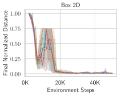
Refer to caption
Refer to caption
Refer to caption
Refer to caption
Refer to caption
Refer to caption
Refer to caption
Figure 5: Ablation results across all six environments. We see that using our derived qTsubscript𝑞𝑇q_{T} optimality equation is important for best performance across all six tasks and that odac is not sensitive to the quality of the dynamics model.
Refer to caption
Refer to caption
t=30𝑡30t=30
Refer to caption
t=40𝑡40t=40
Refer to caption
t=50𝑡50t=50
Figure 7: The inferred qΔt+1(Δt+1=0)subscript𝑞subscriptΔ𝑡1subscriptΔ𝑡10q_{\Delta_{t+1}}(\Delta_{t+1}=0) versus time during an example trajectory in the Ant environment. As the ant robot falls over, qΔt+1(Δt+1=0)subscript𝑞subscriptΔ𝑡1subscriptΔ𝑡10q_{\Delta_{t+1}}(\Delta_{t+1}=0) drops in value. We see that the optimal posterior qΔt+1(Δt+1=0)superscriptsubscript𝑞subscriptΔ𝑡1subscriptΔ𝑡10q_{\Delta_{t+1}}^{\star}(\Delta_{t+1}=0) given in Proposition 2 automatically assigns a high likelihood of terminating when this irrecoverable state is first reached, effectively acting as a dynamic discount factor.

B.2 Comparisons under Oracle Goal Sampling
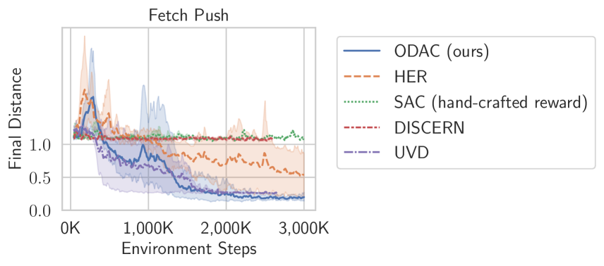
Refer to caption
Figure 8: Comparison of different methods for desired outcomes 𝐠𝐠\mathbf{g} sampled uniformly from the set of admissible states.

For exploration, Andrychowicz et al. [2] explore the benefits of HER either using a single, fixed goal during exploration (see Section 4.3 of Andrychowicz et al. [2]) or using oracle goal sampling, that is, during exploration, a new goal is sampled each episode from a uniform distribution over the set of all reachable goals in the environment. As such, oracle goal sampling requires knowledge of the environment to sample several reachable goals. For example, in the 2D box experiment (Figure 3(a)), points inside the grey block in the center are not reachable goal states, and this additional information must be available when performing oracle goal sampling.

To demonstrate the impact of sampling the desired outcome 𝐠𝐠\mathbf{g} during exploration, we evaluate odac and related methods on the Fetch task when using oracle goal sampling. As shown in Figure 8, the performances of UVD and odac are similar and both outperform other methods. These results suggest that UVD depends more heavily on sampling outcomes from the set of desired outcomes than odac. The significant decrease in performance when the desired outcome 𝐠𝐠\mathbf{g} is fixed may be due to the fact that uniformly sampling 𝐠𝐠\mathbf{g} implicitly provides a curriculum for learning. For example, in the Box 2D environment, goal states sampled above the box can train the agent to move around the obstacle, making it easier to learn how to reach the other side of the box. Without this guidance, prior methods often “get stuck” on the other side of the box. In contrast, odac consistently performs well in this more challenging setting, suggesting that the log-likelihood signal provides good guidance to the policy.

As shown in Figure 4, odac performs well on both this setting and the harder setting where the desired outcome 𝐠𝐠\mathbf{g} was fixed during exploration, suggesting that odac does not rely as heavily on the uniform sampling of 𝐠𝐠\mathbf{g} to learn a good policy than do other methods.

B.3 Comparison to Model-Based Planning

odac learns a dynamics model but does not use it for planning and instead relies on the derived Bellman updates to obtain a policy. However, a natural question is whether or not the method would benefit from using this model to perform model-based planning, as in Janner et al. [21]. We assess this by comparing odac with model-based baseline that uses a 1-step look-ahead. In particular, we follow the training procedure in Janner et al. [21] with k=1𝑘1k=1. To ensure a fair comparison, we use the exact same dynamics model architecture as in odac and match the update-to-environment step ratio to be 4-to-1 for both methods.

Section B.3 shows the final distance to the goal (best results in bold). Using the same dynamics model, odac, which does not use the dynamics model to perform planning and only uses it to compute rewards, outperforms the model-based planning method. While a better model might lead to better performance for the model-based baseline, these results suggest that odac is not sensitive to model quality to the same degree as model-based planning methods.

Table 2: Normalized final distances (lower is better) across four random seeds, multiplied by a factor of 100100100.
Environment odac (Mean + Standard Error) Dyna (Mean + Standard Error)
Box 2D 0.74 (0.091) 0.87 (0.058)
Ant 33 (27) 102 (0.83)
Sawyer Faucet 14 (6.3) 100 (5)
Fetch Push 12 (3.7) 96 (3.8)
Sawyer Push 58 (8.7) 96 (0.39)
Sawyer Window 4.4 (1.5) 116 (14)

B.4 Reward Visualization

We visualize the reward for the Box 2D environment in Figure 9. We see that over the course of training, the reward function initially flattens out near 𝐠𝐠\mathbf{g}, making learning easier by encouraging the policy to focus on moving just out of the top left corner of the environment. Later in training (around 16,000 steps), the policy learns to move out of the top left corner, and we see that the reward changes to have a stronger reward gradient near 𝐠𝐠\mathbf{g}. We also note that the reward are much more negative for being far 𝐠𝐠\mathbf{g} at the end of training: the top left region changes from having a penalty of 1.61.6-1.6 to 107107-107. Overall, these visualizations show that the reward function automatically changes during training and provides a strong reward signal for different parts of the state space depending on the behavior of the policy.
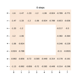
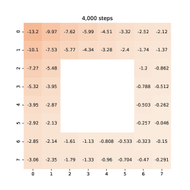
Refer to caption
Refer to caption
Refer to caption
Refer to caption
Refer to caption
Refer to caption
Refer to caption
(a) Reward Visualization
Refer to caption
(b) Learning Curve associated with Reward Visualized
Refer to caption
(c) Environment Visualization
Figure 9: We visualize the rewards over the course of training on a single random seed for the Box 2D environment. To visualize the reward, we discretize the continuous state space and evaluate r(𝐬t,𝐚t,𝐠;qΔ)𝑟subscript𝐬𝑡subscript𝐚𝑡𝐠subscript𝑞Δr(\mathbf{s}_{t},\mathbf{a}_{t},\mathbf{g};q_{\Delta}) for 𝐚=0𝐚0\mathbf{a}=\vec{0} at different states. As shown in Figure 9(c), the desired outcome 𝐠𝐠\mathbf{g} is near the bottom right and the states in the center are invalid. After 4-8 thousand environment steps, the reward is more flat near 𝐠𝐠\mathbf{g}, and only provides a reward gradient far from 𝐠𝐠\mathbf{g}. After 20 thousand environment steps, the reward gradient is much larger again near the end, and the penalty for being in the top left corner has changed from 1.61.6-1.6 to 107107-107.

Appendix C Experimental Details

C.1 Environment

Ant.

This Ant domain is based on the “Ant-V3” OpenAI Gym [4] environment, with three modifications: the gear ratio is reduced from 150150150 to 120120120, the contact force sensors are removed from the state, and there is no termination condition and the episode only terminates after a fixed amount of time. In this environment, the state space is 232323 dimensional, consistent of the XYZ coordinate of the center of the torso, the orientation of the ant (in quaternion), and the angle and angular velocity of all 8 joints. The action space is 8-dimensional and corresponds to the torque to apply to each joint. The desired outcome consists of the desired XYZ, orientation, and joint angles at a position that is 5 meters down and to the right of the initial position. This desired pose is shown in Figure 4.

Sawyer Push.

In this environment, the state and goal space is 444 dimensional and the action space is 222 dimension. The state and goal consists of the XY end effector (EE) and the XY position of the puck. The object is on a 40cm x 50cm table and starts 20 cm in front of the hand. The goal puck position is fixed to 15 cm forward and 30 cm to the right of the initial hand position, while the goal hand position is 5cm behind and 20 cm to the right of the initial hand position. The action is the change in position in each XY direction, with a maximum change of 3 cm per direction at each time step. The episode horizon is 100.

Sawyer Window and Faucet.

In this environment, the state and goal space is 666 dimensional and the action space is 222 dimension. The state and goal consists of the XYZ end effector (EE) and the XYZ position of the window or faucet end endpoint. The hand is initialized away from the window and faucet. The EE goal XYZ position is set to the initial window or faucet position. The action is the change in position in each XYZ direction. For the window task, the goal positions is to close the window, and for the faucet task, the goal position is to rotate the faucet 909090 degrees counter-clockwise from above.

Box 2D.

In this environment, the state is a 4x44𝑥44x4 with a 2x22𝑥22x2 box in the middle. The policy is initialized to to (3.5,2)3.52(-3.5,-2) and the desired outcome is (3.5,2)3.52(3.5,2). The action is the XY velocity of the agent, with wall collisions taken into account and maximum velocity of 0.20.20.2 in each direction. To make the environment stochastic, we add Gaussian noise to actions with mean zero and standard deviation that’s 10% of the maximum action magnitude.

Tabular Box 2D (Figure 1).

We implemented a tabular version of odac and applied it to the 2D environment shown in Figure 3(a). We discretize the environment into an 8×8888\times 8 grid of states. The action correspond to moving up, down, left, or right. If probability 1ϵ1italic-ϵ1-\epsilon, this action is taken. If the agent runs into a wall or boundary, the agent stays in its current state. With probability ϵ=0.1italic-ϵ0.1\epsilon=0.1, the commanded action is ignored and a neighboring state grid (including the current state) is uniformly sampled as the next state. The policy and Q𝑄Q-function are represented with look-up tables and randomly initialized. The entropy reward is weighted by 0.010.010.01 and the time prior pTsubscript𝑝𝑇p_{T} is geometric with parameter 0.50.50.5. The dynamics model, pd(0)superscriptsubscript𝑝𝑑0p_{d}^{(0)} is initialized to give a uniform probability to each states for every state and action. Each iteration, we simulate data collection by updating the dynamics model with the running average update pd(t+1)=0.99pd(t)+0.01pd,superscriptsubscript𝑝𝑑𝑡10.99superscriptsubscript𝑝𝑑𝑡0.01subscript𝑝𝑑p_{d}^{(t+1)}=0.99p_{d}^{(t)}+0.01p_{d}, where pdsubscript𝑝𝑑p_{d} is the true dynamics and update the policy and Q𝑄Q-function according to Equation 16 and Equation 14, respectively. Figure 1 shows that, in contrast to the binary-reward setting, the learned reward provides shaping for the policy, which solves the task within 100 iterations.

C.2 Algorithm

Pseudocode for the complete algorithm is shown in Algorithm 2.

Algorithm 2 Outcome-Driven Actor Critic
0:  Policy πθsubscript𝜋𝜃\pi_{\theta}, Q𝑄Q-function Qϕsubscript𝑄italic-ϕQ_{\phi}, dynamics model pψsubscript𝑝𝜓p_{\psi}, replay buffer \mathcal{R}, and map from state to achieved goal f𝑓f.
  for n=0,N1𝑛0𝑁1n=0,\dots N-1 episodes do
     Sample initial state 𝐬0subscript𝐬0\mathbf{s}_{0} from environment.
     Sample goal 𝐠𝐠\mathbf{g} from environment.
     for t=0,,H1𝑡0𝐻1t=0,\dots,H-1 steps do
        Get action 𝐚tπθ(𝐬t,𝐠)similar-tosubscript𝐚𝑡subscript𝜋𝜃subscript𝐬𝑡𝐠\mathbf{a}_{t}\sim\pi_{\theta}(\mathbf{s}_{t},\mathbf{g}).
        Get next state 𝐬t+1p(|𝐬t,𝐚t)\mathbf{s}_{t+1}\sim p(\cdot\,|\,\mathbf{s}_{t},\mathbf{a}_{t}).
        Store (𝐬t,𝐚t,𝐬t+1,𝐠)subscript𝐬𝑡subscript𝐚𝑡subscript𝐬𝑡1𝐠(\mathbf{s}_{t},\mathbf{a}_{t},\mathbf{s}_{t+1},\mathbf{g}) into replay buffer \mathcal{R}.
        Sample transition (𝐬,𝐚,𝐬,𝐠)similar-to𝐬𝐚superscript𝐬𝐠(\mathbf{s},\mathbf{a},\mathbf{s}^{\prime},\mathbf{g})\sim\mathcal{R}.
        Compute reward r=logpψ(𝐠|𝐬,𝐚)𝔻KL(qΔ(|𝐬t,𝐚t)p(Δ))r=\log p_{\psi}(\mathbf{g}\,|\,\mathbf{s},\mathbf{a})-\mathbb{D}_{\text{KL}}(q_{\Delta}(\cdot|\mathbf{s}_{t},\mathbf{a}_{t})\;\|\;p(\Delta)).
        Compute q(Δt=0|𝐬,𝐚)𝑞subscriptΔ𝑡conditional0𝐬𝐚q(\Delta_{t}=0|\mathbf{s},\mathbf{a}) using Equation 11.
        Update Qϕsubscript𝑄italic-ϕQ_{\phi} using Equation 17 and data (𝐬,𝐚,𝐬,𝐠,r)𝐬𝐚superscript𝐬𝐠𝑟(\mathbf{s},\mathbf{a},\mathbf{s}^{\prime},\mathbf{g},r).
        Update πθsubscript𝜋𝜃\pi_{\theta} using Equation 18 and data (𝐬,𝐚,𝐠)𝐬𝐚𝐠(\mathbf{s},\mathbf{a},\mathbf{g}).
        Update pψsubscript𝑝𝜓p_{\psi} using Equation 19 and data (𝐬,𝐚,𝐠)𝐬𝐚𝐠(\mathbf{s},\mathbf{a},\mathbf{g}).
     end for
     for t=0,,H1𝑡0𝐻1t=0,...,H-1 steps do
        for i=0,,k1𝑖0𝑘1i=0,...,k-1 steps do
           Sample future state 𝐬hisubscript𝐬subscript𝑖\mathbf{s}_{h_{i}}, where t<hiH1𝑡subscript𝑖𝐻1t<h_{i}\leq H-1.
           Store (𝐬t,𝐚t,𝐬t+1,f(𝐬hi))subscript𝐬𝑡subscript𝐚𝑡subscript𝐬𝑡1𝑓subscript𝐬subscript𝑖(\mathbf{s}_{t},\mathbf{a}_{t},\mathbf{s}_{t+1},f(\mathbf{s}_{h_{i}})) into \mathcal{R}.
        end for
     end for
  end for

C.3 Implementation Details

Dynamics model.

For the Ant and Sawyer experiments, we train a neural network to output the mean and standard deviation of a Laplace distribution. This distribution is then used to model the distribution over the difference between the current state and the next state, which we found to be more reliable than predicting the next state. So, the overall distribution is given by a Laplace distribution with learned mean μ𝜇\mu and fixed standard deviation σ𝜎\sigma computed via

pψ=Laplace(μ=gψ(𝐬,𝐚)+f(𝐬),σ=0.00001)subscript𝑝𝜓Laplaceformulae-sequence𝜇subscript𝑔𝜓𝐬𝐚𝑓𝐬𝜎0.00001\displaystyle p_{\psi}=\text{Laplace}(\mu=g_{\psi}(\mathbf{s},\mathbf{a})+f(\mathbf{s}),\sigma=0.00001)

where g𝑔g is the output of a network and f𝑓f is a function that maps a state into a goal.

For the 2D Navigation experiment, we use a Gaussian distribution. The dynamics neural network has hidden units of size [64,64]6464[64,64] with a ReLU hidden activations. For the Ant and Sawyer experiments, there is no output activation. For the linear-Gaussiand and 2D Navigation experiments, we have a tanh output, so that the mean and standard To bound the standard deviation outputted by the network, the standard-deviation tanh is multiplied by two with the standard deviation be between limited to between

Reward normalization.

Because the different experiments have rewards of very different scale, we normalize the rewards by dividing by a running average of the maximum reward magnitude. Specifically, for every reward r𝑟r in the i𝑖ith batch of data, we replace the reward with

r^=r/Ci^𝑟𝑟subscript𝐶𝑖\displaystyle\hat{r}=r/C_{i}

where we update the normalizing coefficient Cisubscript𝐶𝑖C_{i} using each batch of reward {rb}b=1Bsuperscriptsubscriptsubscript𝑟𝑏𝑏1𝐵\{r_{b}\}_{b=1}^{B}:

Ci+1(1λ)×Ci+λmaxb[1,,B]|rb|subscript𝐶𝑖11𝜆subscript𝐶𝑖𝜆subscript𝑏1𝐵subscript𝑟𝑏\displaystyle C_{i+1}\leftarrow(1-\lambda)\times C_{i}+\lambda\max_{b\in[1,\dots,B]}|r_{b}|

and Cisubscript𝐶𝑖C_{i} is initialized to 111. In our experiments, we use λ=0.001𝜆0.001\lambda=0.001.

Target networks.

To train our Q-function, we use the technique from Fujimoto et al. [12] in which we train two separate Q-networks with target networks and take the minimum over two to compute the bootstrap value. The target networks are updated using a slow, moving average of the parameters after every batch of data:

ϕ¯i+1=(1τ)ϕ¯i+×ϕi.\displaystyle\bar{\phi}_{i+1}=(1-\tau)\bar{\phi}_{i}+\times\phi_{i}.

In our experiments, we used τ=0.001𝜏0.001\tau=0.001.

Automatic entropy tuning.

We use the same technique as in Haarnoja et al. [17] to weight the rewards against the policy entropy term. Specifically, we pre-multiply the entropy term in

V^(𝐬,𝐠)Qϕ¯(𝐬,𝐚,𝐠)logπ(𝐚|𝐬;𝐠),^𝑉superscript𝐬𝐠subscript𝑄¯italic-ϕsuperscript𝐬superscript𝐚𝐠𝜋conditionalsuperscript𝐚superscript𝐬𝐠\displaystyle\hat{V}(\mathbf{s}^{\prime},\mathbf{g})\approx Q_{{\bar{\phi}}}(\mathbf{s}^{\prime},\mathbf{a}^{\prime},\mathbf{g})-\log\pi(\mathbf{a}^{\prime}|\mathbf{s}^{\prime};\mathbf{g}),

by a parameter α𝛼\alpha that is updated to ensure that the policy entropy is above a minimum threshold. The parameter α𝛼\alpha is updated by taking a gradient step on the following function with each batch of data:

α(α)=α(logπ(𝐚|𝐬,𝐠)+target)subscript𝛼𝛼𝛼𝜋conditional𝐚𝐬𝐠subscripttarget\displaystyle\mathcal{F}_{\alpha}(\alpha)=-\alpha\left(\log\pi(\mathbf{a}\,|\,\mathbf{s},\mathbf{g})+\mathcal{H}_{\text{target}}\right)

and where targetsubscripttarget\mathcal{H}_{\text{target}} is the target entropy of the policy. We follow the procedure in Haarnoja et al. [17] to choose targetsubscripttarget\mathcal{H}_{\text{target}} and choose target=Dactionsubscripttargetsubscript𝐷action\mathcal{H}_{\text{target}}=-D_{\text{action}}, where Dactionsubscript𝐷actionD_{\text{action}} is the dimension of the action space.

Exploration policy.

Because odac is an off-policy algorithm, we are free to use any exploration policy. It may be beneficial to add For the Ant and Sawyer tasks, we simply sample current policy. For the 2D Navigation task, at each time step, the policy takes a random action with probability 0.3 and repeats its

Evaluation policy.

For evaluation, we use the mean of the learned policy for selecting actions.

Hyperparameters.

Table 4 lists the hyperparameters that were shared across the experiments. Table 3 lists hyper-parameters specific to each environment.

Table 3: Environment specific hyper-parameters.
     Environment      horizon      Q𝑄Q-function and policy network sizes (hidden units)
     Box 2D      100      [64, 64]
     Ant      100      [400, 300]
     Fetch Push      50      [64, 64]
     Sawyer Push      100      [400, 300]
     Sawyer Window      100      [400, 300]
     Sawyer Faucet      100      [400, 300]
Table 4: General hyperparameters used for all experiments.
               Hyperparameter                Value
               # training batches per environment step                111
               batch size                256256256
               discount Factor                0.990.990.99
               policy hidden activation                ReLU
               Q𝑄Q-function hidden activation                ReLU
               replay buffer size                111 million
               hindsight relabeling strategy                future
               hindsight relabeling probability                80%
               target network update speed τ𝜏\tau                0.001
               reward scale update speed λ𝜆\lambda                0.001