A $q$-binomial extension of the CRR asset pricing model

Abstract

We propose an extension of the Cox-Ross-Rubinstein (CRR) model based on $q$-binomial (or Kemp) random walks, with application to default with logistic failure rates. This model allows us to consider time-dependent switching probabilities varying according to a trend parameter on a non-self-similar binomial tree. In particular, it includes tilt and stretch parameters that control increment sizes. Option pricing formulas are written using $q$-binomial coefficients, and we study the convergence of this model to a Black-Scholes type formula in continuous time. A convergence rate of order $O(N^{-1/2})$ is obtained.

Keywords: CRR model, default with logistic failure rate, $q$-binomial coefficients, Kemp random walk, option pricing, weak convergence, continuous-time limit.

Mathematics Subject Classification (2020): 60G42, 60G50, 11B65, 91G20.

JEL Classification: C02, G12, G13, D84, C25, C53.

1 Introduction

The binomial option pricing model was introduced in Sharpe (1978) and established in Cox et al. (1979), based on a recombining binary tree allowing for two different market returns $u$, $d$ at every time step. This model leads to tractable option pricing formulas for vanilla and exotic options using binomial coefficients, that converge to the Black-Scholes pricing formula see e.g. $\S$15-1 of Williams (1991), and § 5.7 of Föllmer and Schied (2004). Although pricing and hedging in the CRR model can be extended to time-dependent parameters, see e.g. § 11.4 in Privault (2009), the corresponding option pricing formulas have exponential instead of polynomial complexity, see also Georgiadis (2011).

Extending the flexibility of the CRR model using a wider class of parameters while maintaining its original polynomial complexity has important consequences for financial modeling. As the CRR model uses constant switching probabilities over time, it does not account possible acceleration effects in economic recessions or recoveries. For example, investors may overreact to a bad performance of a stock, and become more sensitive to a decrease in the underlying asset prices, see e.g. Soroka (2006). In this paper, we construct a CRR type model based on a $q$-binomial random walk with time-dependent switching probabilities, by replacing standard binomial coefficients with $q$-binomial coefficients. This provides an alternative to the binomial model by maintaining its polynomial complexity and by allowing the underlying security to move up and down with probabilities increasing or decreasing according to a trend parameter. This feature allows us to model default probabilities in a model where default risk can be compounded into a failure rate which can increase or decrease over time according to a logistic expression. This can for example apply to the modeling of accelerating economic recession or expansion phases. In addition, this model allows for the inclusion of a stretch parameter.

Convergence of approximations in the continuous-time limit is another important issue. Convergence rates of the order $O(N^{-1})$ in the number of time steps for the price of European call options have been obtained in Leisen and Reimer (1996) for the model of Tian (1993), see also Diener and Diener (2004) for a general asymptotic expansion for call options prices in the CRR model. In Tian (1999), a flexible CRR model with an additional “tilt” parameter has been proposed, and extended in Chang and Palmer (2007) as a general class of binomial models with a drift parameter that yields smooth convergence at the rate $O(N^{-1})$, with expansions in powers of $1/\sqrt{N}$ for the prices of digital and vanilla put and call options. In addition, arbitrarily fast convergence in binomial trees has been achieved in Joshi (2010) and Xiao (2010) respectively for odd and even number of time steps, and in Leduc (2013) for the model of Chang and Palmer (2007).

An optimal-drift model further reducing the order of convergence of the discretisation error from $O(N^{-1})$ to $o(N^{-1})$ has been proposed in Korn and Müller (2013). As noted in Leduc (2016b), such high-order convergence results cannot be reached when the strike price is too far away from the spot price. It has also been shown in Leduc (2016a) that as the number $N$ of time steps tends to infinity, the order of convergence of tree-based methods is in general $O(N^{-1})$ for continuous payoff functions, and $O(1/\sqrt{N})$ otherwise. See also Heston and Zhou (2000) for related “local” convergence rates, and Walsh (2003) for expressions of the coefficients of $1/\sqrt{N}$ and $1/N$ in the expansion of options prices with general payoff functions in a CRR-related model.

In Ritchken (1995), an additional “stretch” parameters has been introduced for the fine tuning of the pricing of barrier options in the trinomial model. In Chung and Shih (2007) the convergence of such a generalized CRR (GCRR) model has been studied, and has been shown to be of order $O(1/\sqrt{N})$ in the presence of stretch, and of order $O(N^{-1})$ without stretch, see Theorem 2 therein. Convergence of order $O(N^{-1})$ is also obtained in Chung and Shih (2007) for a suitable sequence of stretch parameters converging to one, see Corollary 1 therein.

Our $q$-binomial model also includes an additional parameter $\theta>0$, see (2.1) below, which plays the role of a stretch parameter. In order to evaluate the continuous-time limit of our model in option pricing, we will derive convergence results for $q$-binomial random walks. As noted in Charalambides (2016), the central limit theorem does not hold for the $q$-binomial distribution. On the other hand, the convergence of the $q$-binomial distribution has been studied for fixed $q\in(0,1)$, and convergence to a discrete Heine distribution has been shown in Gerhold and Zeiner (2010), see also Kyriakoussis and Vamvakari (2013).

In our financial setting we consider the case where $q=q_{N}$ depends on the total number of steps $N$, and study the convergence of the $q_{N}$-binomial model on $\{0,1,\ldots,N\}$ when $q_{N}$ tends to one as $N$ tends to infinity. In this setting, we show in Theorem 4.1 that when $q_{N}$ takes the form

$$q_{N}:=1+\eta\left(\frac{T}{N}\right)^{3/2}+O(N^{-2})$$

for some $T>0$, where the parameter $\eta\in$ captures the “intensity” of the trend $q_{N}$, and the market returns $d_{N}$, $u_{N}$ satisfy

$$d_{N}:=1-\sigma\sqrt{\frac{\theta T}{N}}+\zeta\sigma^{2}\frac{\theta T}{2N}+o(N^{-1}),\quad u_{N}:=1+\sigma\sqrt{\frac{\theta T}{N}}+\zeta\sigma^{2}\frac{\theta T}{2N}+o(N^{-1}),\quad$$

this model converges to a continuous-time (generalized) Black-Scholes price model of the type

$$d\macc@depth\char 1\relax\frozen@everymath{\macc@group}\macc@set@skewchar\macc@nested@a 111{S}_{t}=\sigma\macc@depth\char 1\relax\frozen@everymath{\macc@group}\macc@set@skewchar\macc@nested@a 111{S}_{t}dB_{t}+\zeta\frac{\sigma^{2}}{2}\macc@depth\char 1\relax\frozen@everymath{\macc@group}\macc@set@skewchar\macc@nested@a 111{S}_{t}dt+\frac{\sigma\eta\sqrt{\theta}}{1+\theta}t\macc@depth\char 1\relax\frozen@everymath{\macc@group}\macc@set@skewchar\macc@nested@a 111{S}_{t}dt,$$

with time-dependent affine interest rate on $[0,T]$, where $(B_{t})_{t\in[0,T]}$ is a standard Brownian motion. This result is proved in the sense weak convergence on the Skorohod space $\mathbb{D}([0,T],\mathbb{R})$ of càdlàg functions, equipped with the $J_{1}$ topology given by the distance

$$d_{J_{1}}(x,y)=\inf_{\lambda\in\Lambda}\big{(}\|x-(y\circ\lambda)\|_{\infty}+\|{\rm Id}-\lambda\|_{\infty}\big{)},\quad x,y\in\mathbb{D}([0,T],\mathbb{R}),$$

where ${\rm Id}$ denotes identity, $\|x\|_{\infty}=\sup_{t\in[0,T]}|x(t)|$, and $\Lambda$ denotes the set of strictly increasing mappings $\lambda$ of $[0,T]$ onto itself, see (Billingsley 1999, Section 12). In addition, in Theorem 3.1 we show convergence of European option prices at the rate $O(N^{-1/2})$. For this, we use an expansion for the distribution of sums of non identically distributed Bernoulli random variables, see Theorem 1.3 in Deheuvels et al. (1989), which extends Uspensky’s theorem, see § VII-11 of Uspensky (1937), which applied to i.i.d. case.

We proceed as follows. In Section 2 we review the main properties of $q$-binomial distributions and we prove a central limit theorem for the associated $q$-binomial random walk. Our $q$-binomial extension of the CRR model is presented in Section 3. Theorem 3.1 shows the weak convergence of our model to a generalized Black-Scholes model using a geometric Brownian motion with affine time-dependent drift, with convergence rates of order $O(N^{-1/2})$ or $O(N^{-1})$ depending on the model parameters. Theorem 3.1 is proved in Sections 4-5 by studying the weak convergence of the $q$-binomial random walk in continuous time.

2 The $q$-binomial distribution

This section contains the basic knowledge on $q$-binomial distribution and random walk that will be needed in the sequel. Consider the sequence $(X_{k})_{k\geq 1}$ of independent Bernoulli random variables with variable distribution parameterized in the logistic form

$${\mathord{\mathbb{P}}}_{\theta,q}(X_{k}=0)=\frac{1}{1+\theta q^{k-1}}\quad\mbox{and}\quad{\mathord{\mathbb{P}}}_{\theta,q}(X_{k}=1)=\frac{\theta q^{k-1}}{1+\theta q^{k-1}},$$ (2.1)

$k\geq 1$, where $\theta,q>0$, see Berkson (1953), Cox (1958). This parametrization has been used in Kemp and Kemp (1991) to construct the following extension of the binomial distribution with application to the statistical study of dice rolling experiments. This distribution is also derived in e.g. Corollary 3.1 of Charalambides (2010) and Theorem 9.5 of Charalambides (2019). In the next proposition we consider the time-inhomogeneous random walk $(Z_{n})_{n\geq 0}$ associated to the $q$-binomial distribution.

Proposition 2.1

Let $(X_{k})_{k\geq 1}$ be a sequence of independent Bernoulli random variables with distribution (2.1). The sum

$$Z_{n}:=X_{1}+\cdots+X_{n},\qquad n\geq 1,$$

with $Z_{0}:=0$, has the distribution

$${\mathord{\mathbb{P}}}_{\theta,q}(Z_{N}-Z_{n}=k)=\frac{\theta^{k}q^{(2n+k-1)k/2}}{(1+\theta q^{n})(1+\theta q^{n+1})\cdots(1+\theta q^{N-1})}{N-n\choose k}_{q},$$ (2.2)

$k=0,1,\ldots,N-n$, $0\leq n\leq N$, and the probability generating function

$$\mathop{\hbox{\rm I\kern-1.99997ptE}}\nolimits_{\theta,q}\big{[}t^{Z_{n}}\big{]}=\frac{(1+\theta tq)\cdots(1+\theta tq^{n-1})}{(1+\theta q)\cdots(1+\theta q^{n-1})},\qquad t\in[0,1],$$

where

$${n\choose k}_{q}:=\frac{(1-q^{n})\cdots(1-q^{n-k+1})}{(1-q)\cdots(1-q^{k})},\qquad k=0,1,\ldots,n,$$

is the $q$-binomial, or Gaussian binomial, coefficient.

Proof. For completeness, we provide a proof by induction on $N\geq n$. Relation (2.2) is clearly satisfied for $N=n$ and $N=n+1$. Assuming that (2.2) is satisfied at the rank $n\geq N$, we have

$$\!\!\!\!\!\!\!{\mathord{\mathbb{P}}}_{\theta,q}(Z_{N+1}-Z_{n}=k)=\frac{1}{1+\theta q^{N}}{\mathord{\mathbb{P}}}_{\theta,q}(Z_{N}-Z_{n}=k)+\frac{\theta q^{N}}{1+\theta q^{N}}{\mathord{\mathbb{P}}}_{\theta,q}(Z_{N}-Z_{n}=k-1)$$

$$= \frac{1}{(1+\theta q^{N})}\frac{\theta^{k}q^{(2n+k-1)k/2}}{(1+\theta q^{n})(1+\theta q^{n+1})\cdots(1+\theta q^{N-1})}{N-n\choose k}_{q}$$

$$+\frac{\theta q^{N}}{(1+\theta q^{N})}\frac{\theta^{k-1}q^{(2n+k-1)(k-2)/2}}{(1+\theta q^{n})(1+\theta q^{n+1})\cdots(1+\theta q^{N-1})}{N-n\choose k-1}_{q}$$

$$= \frac{\theta^{k}q^{(2n+k-1)k/2}}{(1+\theta q^{n})(1+\theta q^{n+1})\cdots(1+\theta q^{N})}\left({N-n\choose k}_{q}+q^{N-n-(k-1)}{N-n\choose k-1}_{q}\right)$$

$$= \frac{\theta^{k}q^{(2n+k-1)k/2}}{(1+\theta q^{n})(1+\theta q^{n+1})\cdots(1+\theta q^{N})}{N+1-n\choose k}_{q},$$

where we applied the $q$-Pascal rule

$${N+1-n\choose k}_{q}={N-n\choose k}_{q}+q^{N-n-(k-1)}{N-n\choose k-1}_{q},$$

see Proposition 6.1 in Kac and Cheung (2002). Next, regarding the probability generating function, we have

$$\mathop{\hbox{\rm I\kern-1.99997ptE}}\nolimits_{\theta,q}\big{[}t^{Z_{n}}\big{]} = \sum_{k=0}^{n}t^{k}{\mathord{\mathbb{P}}}_{\theta,q}(Z_{n}=k)$$

$$= \sum_{k=0}^{n}\frac{(\theta t)^{k}q^{(k-1)k/2}}{(1+\theta)(1+\theta q)\cdots(1+\theta q^{n-1})}{n\choose k}_{q}$$

$$= \left(\prod_{l=1}^{n}\frac{1}{1+\theta q^{l-1}}\right)\sum_{k=0}^{n}(\theta t)^{k}q^{(k-1)k/2}{n\choose k}_{q}$$

$$= \prod_{l=1}^{n}\frac{1+\theta tq^{l-1}}{1+\theta q^{l-1}},$$

where we used Gauss’s binomial formula

$$\sum_{k=0}^{n}(\theta t)^{k}q^{(k-1)k/2}{n\choose k}_{q}=\prod_{l=1}^{n}(1+\theta tq^{l-1}),$$

see Relation (5.5) in Kac and Cheung (2002). $\square$

The $q$-binomial distribution reduces to the binomial distribution as $q$ tends to $1$, since the $q$-binomial coefficients converge to the standard binomial coefficients when $q$ tends to $1$, see e.g. Chapter 6 of Kac and Cheung (2002).

Central limit theorem

As noted in Example 5.5 of Charalambides (2016), the central limit theorem does not hold for the $q$-binomial distribution when $q\not=1$, as in this case we have

$$\lim_{N\to\infty}\mathop{\hbox{\rm Var}}\nolimits_{\theta,q}[Z_{N}]=\lim_{N\to\infty}\sum_{k=1}^{N}{\mathord{\mathbb{P}}}_{\theta,q}(X_{k}=0){\mathord{\mathbb{P}}}_{\theta,q}(X_{k}=1)=\lim_{N\to\infty}\sum_{k=1}^{N}\frac{\theta q^{k-1}}{(1+\theta q^{k-1})^{2}}<\infty,$$

see, e.g., Theorem 1.1 in Deheuvels et al. (1989). It has been shown in Gerhold and Zeiner (2010) that for fixed $q\in(0,1)$, the distribution of $Z_{N}$ converges to a discrete Heine distribution as $N$ tends to infinity, see also §10.8.1 in Johnson et al. (2005). In Theorem 2 of Kyriakoussis and Vamvakari (2013), it has been shown that when $\theta$ takes the form $\theta_{N}=q^{-\vartheta N}$ for some $\vartheta\in(0,1)$, the distribution of $Z_{N}$ can be approximated by a deformed Stieltjes-Wigert distribution as $N$ tends to infinity. However, this requires ${\mathord{\mathbb{P}}}_{\theta_{N},q}(Z_{n}=k)$ to tend to zero for $k=1,\ldots,n-1$, which may not be meaningful in a financial setting. In the sequel, we will study the convergence of the $q$-binomial model on $\{1,\ldots,N\}$ when the parameter $q$ depends on $N$ and tends to one as $N$ tends to infinity.

In the next proposition, we show that the $q$-binomial random walk converges to a Gaussian distribution under a suitable assumption on $q_{N}$.

Proposition 2.2

Assume that $q_{N}=1+O(N^{-3/2})$ as $N$ tends to infinity. Then, letting $Z_{N}:=X_{1}+\cdots+X_{N}$, $N\geq 1$, the normalized sequence $(Z_{N}-\mathop{\hbox{\rm I\kern-1.99997ptE}}\nolimits_{\theta,q_{N}}[Z_{N}])/\sqrt{N}$ converges in distribution to a Gaussian ${\cal N}(0,\theta/(1+\theta)^{2})$ random variable as $N$ tends to infinity.

Proof. For $1\leq k\leq N$, by the binomial theorem, we have

$$q_{N}^{k-1}=1+(k-1)O(N^{-3/2})+R^{(k)}_{N},$$

where

$$\big{|}R^{(k)}_{N}\big{|} = \left|\sum_{l=2}^{k-1}{k-1\choose l}(O(N^{-3/2}))^{l}\right|$$

$$= \sum_{l=0}^{k-3}{k-1\choose l+2}|O(N^{-3(l+2)/2})|$$

$$\leq \frac{1}{N}\sum_{l=0}^{k-3}{k-3\choose l}|O(N^{-3l/2})|$$

$$= \frac{1}{N}(1+|O(N^{-3/2})|)^{k-3}$$

$$\leq \frac{1}{N}(1+|O(N^{-3/2})|)^{N}$$

$$= O(N^{-1}).$$

Therefore, we have

$$q_{N}^{k-1}=1+kO(N^{-3/2})+O(N^{-1}),$$

where the above terms $O(N^{-3/2})$ and $O(N^{-1})$ are uniform in $k\in\{1,\ldots,N\}$, hence

$${\mathord{\mathbb{P}}}_{\theta,q_{N}}(X_{k}=1) = \frac{\theta q^{k-1}_{N}}{1+\theta q^{k-1}_{N}}$$ (2.3)

$$= \theta\frac{1+kO(N^{-3/2})+O(N^{-1})}{1+\theta+\theta kO(N^{-3/2})+O(N^{-1})}$$

$$= \frac{\theta}{1+\theta}\big{(}1+kO(N^{-3/2})+O(N^{-1})\big{)}\left(1-\frac{\theta}{1+\theta}kO(N^{-3/2})+O(N^{-1})\right)$$

$$= \frac{\theta}{1+\theta}+\frac{k\theta}{(1+\theta)^{2}}O(N^{-3/2})+O(N^{-1}).$$

Thus, we have

$$\mathop{\hbox{\rm I\kern-1.99997ptE}}\nolimits_{\theta,q_{N}}[Z_{N}] = \sum_{k=1}^{N}{\mathord{\mathbb{P}}}_{\theta,q_{N}}(X_{k}=1)$$

$$= \frac{\theta}{1+\theta}\sum_{k=1}^{N}\left(1+\frac{k}{1+\theta}O(N^{-3/2})+O(N^{-1})\right)$$

$$= \frac{\theta N}{1+\theta}+\frac{\theta O(N^{1/2})}{2(1+\theta)^{2}}+O(1).$$

The variance of $Z_{N}$ is then given by

$$\sigma_{N}^{2}:=\mathop{\hbox{\rm Var}}\nolimits_{\theta,q_{N}}[Z_{N}]=\sum\limits_{k=1}^{N}{\mathord{\mathbb{P}}}_{\theta,q_{N}}(X_{k}=0){\mathord{\mathbb{P}}}_{\theta,q_{N}}(X_{k}=1)$$

$$=\sum\limits_{k=1}^{N}\left(\frac{\theta}{1+\theta}+kO(N^{-3/2})+O(N^{-1})\right)\left(\frac{1}{1+\theta}-kO(N^{-3/2})+O(N^{-1})\right)$$

$$=\frac{\theta N}{(1+\theta)^{2}}+O(N^{1/2})$$ (2.4)

as $N$ tends to infinity, and we conclude by the Lindeberg-Feller central limit theorem, as in e.g. Theorem 1.1 of Deheuvels et al. (1989). $\square$

$q$-geometric distribution

We end this section with some comments on the $q$-geometric distribution associated to the $q$-binomial distribution. Let $\tau$ denote the time the first “$0$” appears in the sequence $(X_{k})_{k\geq 1}$, i.e.

$$\tau:=\inf\{k\geq 1\ :\ X_{k}=0\}.$$

We have

$${\mathord{\mathbb{P}}}_{\theta,q}(\tau\geq k)=\prod_{l=1}^{k-1}{\mathord{\mathbb{P}}}_{\theta,q}(X_{l}=1)=\prod_{l=1}^{k-1}\frac{\theta q^{l-1}}{1+\theta q^{l-1}},\qquad k\geq 1,$$

with $\prod_{l=1}^{0}=1$ by convention, and

$${\mathord{\mathbb{P}}}_{\theta,q}(\tau=k) = {\mathord{\mathbb{P}}}_{\theta,q}(\tau\geq k)-{\mathord{\mathbb{P}}}_{\theta,q}(\tau>k)$$

$$= \prod_{l=1}^{k-1}\frac{\theta q^{l-1}}{1+\theta q^{l-1}}-\prod_{l=1}^{k}\frac{\theta q^{l-1}}{1+\theta q^{l-1}}$$

$$= \frac{1}{1+\theta q^{k-1}}\prod_{l=1}^{k-1}\frac{\theta q^{l-1}}{1+\theta q^{l-1}},\qquad k\geq 1,$$

which is the $q$-geometric distribution of the first kind according to § 2.10 in Charalambides (2016), and yields the standard geometric distribution with parameter $\theta/(1+\theta)$ when $q=1$. Taking $\tau$ as default time, this yields the discrete-time logistic failure rate

$${\mathord{\mathbb{P}}}_{\theta,q}(\tau=k\mid\tau\geq k)=\frac{{\mathord{\mathbb{P}}}_{\theta,q}(\tau=k)}{{\mathord{\mathbb{P}}}_{\theta,q}(\tau\geq k)}=\frac{1}{1+\theta q^{k-1}},\qquad k\geq 1,$$ (2.5)

see (21) in Cox (1972), (7) in Thompson (1977), or (0.8) in Fahrmeir (1997). This rate is constant in the geometric case, and increasing (resp. decreasing) when $q<1$ (resp. $q>1$).

3 A $q$-binomial CRR Model

Given $d,u$ such that $0<d<u$, we consider a risky asset price with initial value $S_{0}$ given in discrete time as

$$S_{n}=S_{0}u^{Z_{n}}d^{n-Z_{n}}=\left\{\begin{array}[]{ll}uS_{n-1},&X_{n}=1,\\ \\ dS_{n-1},&X_{n}=0,\end{array}\right.$$

$n\geq 1$, where $(X_{k})_{k\geq 1}$ is as in (2.1), with the distribution

$${\mathord{\mathbb{P}}}_{\theta,q}(S_{n}=S_{0}u^{k}d^{n-k})=\frac{\theta^{k}q^{(k-1)k/2}}{(1+\theta)(1+\theta q)\cdots(1+\theta q^{n-1})}{n\choose k}_{q},\quad k=0,1,\ldots,n,$$

and

$$\mathop{\hbox{\rm I\kern-1.99997ptE}}\nolimits_{\theta,q}\left[\frac{S_{n}}{S_{n-1}}\right]=\frac{d+u\theta q^{n-1}}{1+\theta q^{n-1}},\quad\mathop{\hbox{\rm Var}}\nolimits_{\theta,q}\left[\frac{S_{n}}{S_{n-1}}\right]=(u-d)^{2}\mathop{\hbox{\rm Var}}\nolimits_{\theta,q}[X_{n}]=\frac{(u-d)^{2}\theta q^{n-1}}{(1+\theta q^{n-1})^{2}},$$ (3.1)

$n\geq 1$. From (2.1), we note that the case $q>1$ is modeling an upward market trend, while $q<1$ models a downward trend. On the other hand, letting $q$ tend to $1$ recovers the standard CRR model with probabilities $1/(1+\theta)$ and $\theta/(1+\theta)$.

Consider now a riskless asset priced $A_{0}=1$ at time $0$ and

$$A_{n}:=\prod_{k=1}^{n}(1+r_{k})$$

at time $n\geq 1$, where $r_{k}$ satisfies

$$1+r_{k}=\mathop{\hbox{\rm I\kern-1.99997ptE}}\nolimits_{\theta,q}\left[\frac{S_{k}}{S_{k-1}}\right]=\frac{d+u\theta q^{k-1}}{1+\theta q^{k-1}},\qquad k\geq 1.$$ (3.2)

As a consequence of (3.1), we find that the discounted price process

$$\widetilde{S}_{n}=\frac{S_{n}}{A_{n}}=S_{n}\prod_{k=1}^{n}(1+r_{k})^{-1},\qquad n\geq 0,$$

is a martingale with respect to the filtration $({\cal F}_{n})_{n\geq 0}$ generated by $(S_{n})_{n\geq 0}$. Therefore, ${\mathord{\mathbb{P}}}_{\theta,q}$ is the unique risk-neutral probability measure and therefore the market model is without arbitrage and complete, see e.g. Theorems 5.17 and 5.38 in Föllmer and Schied (2004).

In this setting, the arbitrage-free price at time $n=0,1,\ldots,N$ of an option with payoff $\phi(S_{N})$ and maturity $N$ is given from (2.2) by

$$\left(\prod_{k=n+1}^{N}(1+r_{k})^{-1}\right)\mathop{\hbox{\rm I\kern-1.99997ptE}}\nolimits_{\theta,q}[\phi(S_{N})\mid{\cal F}_{n}]$$

$$= \left(\prod_{k=n+1}^{N}(1+r_{k})^{-1}\right)\sum_{k=0}^{N-n}\phi(S_{n}u^{k}d^{N-n-k}){\mathord{\mathbb{P}}}_{\theta,q}(Z_{N}-Z_{n}=k)$$

$$= \sum_{k=0}^{N-n}\theta^{k}\frac{q^{(2n+k-1)k/2}\phi(S_{n}u^{k}d^{N-n-k})}{(d+\theta uq^{n})\cdots(d+\theta uq^{N-1})}{N-n\choose k}_{q}.$$

In addition, (2.5) shows that the $q$-binomial model has the ability to model accelerating economic recession or expansion phases.

In the sequel we will study the convergence speed of the discrete $q$-binomial approximation in the case of European call options by defining $q_{N}$, $d_{N}$, $u_{N}$, $r_{k,N}$, $0\leq k\leq N$, as

$$\left\{\begin{array}[]{l}\displaystyle q_{N}:=1+\eta(\Delta t)^{3/2}+O(N^{-2}),\vskip 6.0pt plus 2.0pt minus 2.0pt\\ \displaystyle d_{N}:=1-\sigma\sqrt{\theta\Delta t}+\zeta\sigma^{2}\theta\Delta t/2+o(N^{-3/2}),\vskip 6.0pt plus 2.0pt minus 2.0pt\\ \displaystyle u_{N}:=1+\sigma\sqrt{\Delta t/\theta}+\zeta\sigma^{2}\Delta t/(2\theta)+o(N^{-3/2}),\vskip 6.0pt plus 2.0pt minus 2.0pt\\ \displaystyle r_{k,N}=\frac{d_{N}-1+(u_{N}-1)\theta q_{N}^{k-1}}{1+\theta q_{N}^{k-1}},\qquad k\geq 1.\end{array}\right.$$ (3.3)

As a consequence of Proposition 2.2 or Theorem 4.1 below, it can be shown that the arbitrage-free price

$$\left(\prod_{k=n+1}^{N}(1+r_{k,N})^{-1}\right)\mathop{\hbox{\rm I\kern-1.99997ptE}}\nolimits_{\theta,q}[(S_{N,N}-K)^{+}\mid{\cal F}_{n}]$$

of a European call option with strike price $K$ converges to the continuous-time limit

$$\exp\left(-\zeta\frac{\sigma^{2}}{2}T-\frac{\sigma\eta T^{2}\sqrt{\theta}}{2(1+\theta)}\right)\mathop{\hbox{\rm I\kern-1.99997ptE}}\nolimits\big{[}\big{(}\macc@depth\char 1\relax\frozen@everymath{\macc@group}\macc@set@skewchar\macc@nested@a 111{S}_{T}-K\big{)}^{+}\big{]}=S_{0}\Phi(d_{+})-K\exp\left(-\zeta\frac{\sigma^{2}}{2}T-\frac{\sigma T^{2}\eta\sqrt{\theta}}{2(1+\theta)}\right)\Phi(d_{-})$$ (3.4)

as $N$ tends to infinity, where

$$d_{+}:=\frac{1}{\sigma\sqrt{T}}\left(\log\left(\frac{S_{0}}{K}\right)+(1+\zeta)\frac{\sigma^{2}T}{2}+\frac{\sigma\eta T^{2}\sqrt{\theta}}{2(1+\theta)}\right),\qquad d_{-}=d_{+}-\sigma\sqrt{T},$$

and $\Phi$ is the cumulative distribution function of the standard normal distribution.

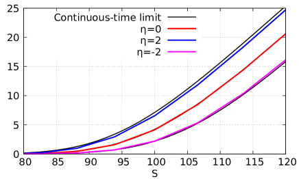
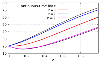
Figure 1 shows European call prices with strike level $K$ as functions of the underlying $S$ and volatility paramter $\sigma$ for $\eta=-2,2$, compared with the CRR and Black-Scholes formulas ($\eta=0$). We note that option prices may not be monotone functions of volatility when $\eta<0$.

(a) Prices with $K=100$, $\sigma=0.1$.

(b) Prices with $S=100$, $K=80$.

Figure 1: Option price graphs with $\theta=\zeta=1$.

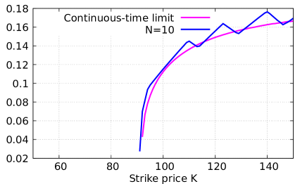
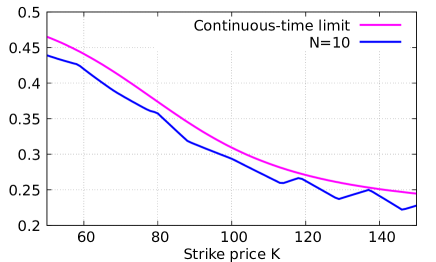
Figure 2 shows the smiles obtained by respectively applying the implied volatilities of the above discrete-time pricing formula and its continuous limit to the CRR and (generalized) Black-Scholes formulas (3.4) with $\eta=0$. We note that this composition may not be always defined when $\eta<0$.

(a) Implied volatility for $\eta=-2$.

(b) Implied volatility for $\eta=2$.

Figure 2: Implied volatility graphs with $\theta=\zeta=1$, $S=100$, $T=1$ and $\sigma=0.2$.

The following result, which is proved in Sections 4-5, provides convergence rates for option prices, see also Remark 5.1.

Theorem 3.1

Let $r_{k,N}$, $d_{N}$, $u_{N}$, and $q_{N}$ be as in (3.3). Then, we have

$$\prod_{k=1}^{N}(1+r_{k,N})^{-1}\mathop{\hbox{\rm I\kern-1.99997ptE}}\nolimits_{\theta,q_{N}}[(S_{N,N}-K)^{+}]$$

$$= \displaystyle S_{0}\Phi(d_{+})-K\exp\left(-\zeta\frac{\sigma^{2}T}{2}-\frac{\sigma\eta T^{2}\sqrt{\theta}}{2(1+\theta)}\right)\Phi(d_{-})+O(N^{-1/2}),$$

as $N$ tends to infinity.

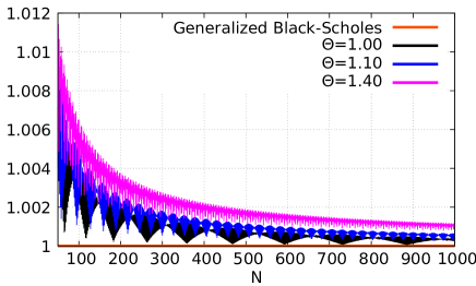
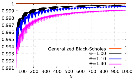
Figure 3 shows the convergence of option prices normalized to $1$ with the parameters $S_{0}=100$, $K=95$, $t=0.5$, $\sigma=0.2$, $T=1$ used in Tian (1999) and Chung and Shih (2007), and $\zeta=1$.

(a) Convergence for $\eta=-1$.

(b) Convergence for $\eta=1$.

Figure 3: Normalized convergence graphs.

Table 1 presents numerical estimates for the graphs of Figure 3.

		Number of time steps
Parameters		$N=100$	$N=1000$	$N=10000$	Limit (3.4)
$\eta=1$	$\theta=1$	11.164676	11.187615	11.189429	11.189701
	$\theta=1.1$	1.228880	11.253394	11.255885	11.256045
$\eta=0$	$\theta=1$	8.949356	8.947683	8.947027	8.947041
	$\theta=1.1$	8.960038	8.947035	8.947104	8.947041
$\eta=-1$	$\theta=1$	7.008068	6.993345	6.991934	6.991621
	$\theta=1.1$	7.027543	6.995757	6.994490	6.993759

Table 1: Convergence table.

4 Weak convergence in continuous time

In the sequel we let $T>0$ denote a terminal time horizon, and we use the discretization $\Delta t:=T/N$ of the time axis. Given $\sigma,\theta>0$ and $\zeta\in$, we assume that

$$d_{N}:=1-\sigma\sqrt{\theta\Delta t}+\zeta\frac{\sigma^{2}}{2}\theta\Delta t+o(N^{-1})\quad\mbox{and}\quad u_{N}:=1+\sigma\sqrt{\frac{\Delta t}{\theta}}+\zeta\frac{\sigma^{2}}{2\theta}\Delta t+o(N^{-1}).$$ (4.1)

In the next proposition we show the convergence of the $q$-binomial model to a (generalized) continuous-time Black-Scholes model with affine time-dependent risk-free interest rate

$$r_{t}:=\zeta\frac{\sigma^{2}}{2}+\frac{\sigma\eta\sqrt{\theta}}{1+\theta}t,\qquad t>0,$$

as the number $N$ of time steps tends to infinity. In the sequel, we let $S_{0,N}:=S_{0}$ and

$$S_{k,N}:=S_{0}u_{N}^{Z_{k}}d_{N}^{k-Z_{k}},\qquad k=1,\ldots,N,$$

and let $\lfloor x\rfloor$ denote the integer part of $x\geq 0$, i.e. the greatest integer less than or equal to $x$.

In the next proposition, we prove that the stepwise interpolation $S_{\lfloor Nt/T\rfloor,N}$, $t\in[0,T]$, between the random variables $S_{k,N}$, $k=0,\ldots,N$, converges to the solution $\big{(}\macc@depth\char 1\relax\frozen@everymath{\macc@group}\macc@set@skewchar\macc@nested@a 111{S}_{t}\big{)}_{t\in[0,T]}$ of the stochastic differential equation

$$d\macc@depth\char 1\relax\frozen@everymath{\macc@group}\macc@set@skewchar\macc@nested@a 111{S}_{t}=\sigma\macc@depth\char 1\relax\frozen@everymath{\macc@group}\macc@set@skewchar\macc@nested@a 111{S}_{t}dB_{t}+\zeta\frac{\sigma^{2}}{2}\macc@depth\char 1\relax\frozen@everymath{\macc@group}\macc@set@skewchar\macc@nested@a 111{S}_{t}dt+\frac{\sigma\eta\sqrt{\theta}}{1+\theta}t\macc@depth\char 1\relax\frozen@everymath{\macc@group}\macc@set@skewchar\macc@nested@a 111{S}_{t}dt,$$

where $(B_{t})_{t\in[0,T]}$ is a standard Brownian motion. The choice of the power $3/2$ in (4.2) is necessary in order for the next result to hold.

Theorem 4.1

Let $d_{N}$, $u_{N}$ be as in (4.1), and assume that $q_{N}$ depends on $N$ as

$$q_{N}:=1+\eta(\Delta t)^{3/2}+O(N^{-2}),$$ (4.2)

where $\eta\in$ and $\Delta t:=T/N$. Then we have the weak convergence

$$\left(S_{\lfloor Nt/T\rfloor,N}\right)_{t\in[0,T]}\ext@arrow 0359\Rightarrowfill@{}{\mathbb{D}([0,T],\mathbb{R})}\left(S_{0}\exp\left(\frac{\sigma\eta\sqrt{\theta}}{2(1+\theta)}t^{2}-(1-\zeta)\frac{\sigma^{2}}{2}t+\sigma B_{t}\right)\right)_{t\in[0,T]}$$

in $\mathbb{D}([0,T],\mathbb{R})$ as $N$ tends to infinity.

Proof. We start by proving one-dimensional convergence, followed by finite-dimensional convergence, and we conclude by showing the tightness of the sequence $\left(S_{\lfloor Nt/T\rfloor,N}\right)_{t\in[0,T]}$. We note that weak convergence can be obtained as a consequence of one-dimensional convergence for time-homogeneous Markov processes, see e.g. Theorems 2.5-2.6 of Ethier and Kurtz (2005), however, we prefer to present a self-contained proof here, as our random walk is not time-homogeneous. First, we show that for any $t\in[0,T]$ the one-dimensional convergence

$$S_{\lfloor Nt/T\rfloor,N}\ext@arrow 0359\Rightarrowfill@{}{\displaystyle}S_{0}\exp\left(\frac{\sigma\eta\sqrt{\theta}}{2(1+\theta)}t^{2}-(1-\zeta)\frac{\sigma^{2}}{2}t+\sigma B_{t}\right)$$ (4.3)

holds in distribution as $N$ tends to infinity. We note that

$$\frac{u_{N}}{d_{N}}=\left(1+\sigma\sqrt{\frac{\Delta t}{\theta}}+\zeta\frac{\sigma^{2}}{2\theta}\Delta t+o(N^{-1})\right)\left(1-\sigma\sqrt{\theta\Delta t}+\zeta\frac{\sigma^{2}}{2}\theta\Delta t+o(N^{-1})\right)^{-1}$$ (4.4)

$$= \left(1+\sigma\sqrt{\frac{\Delta t}{\theta}}+\zeta\frac{\sigma^{2}}{2\theta}\Delta t+o(N^{-1})\right)\left(1+\sigma\sqrt{\theta\Delta t}+\Big{(}1-\frac{\zeta}{2}\Big{)}\sigma^{2}\theta\Delta t+o(N^{-1})\right)$$

$$= 1+\sigma\frac{\theta+1}{\sqrt{\theta}}\sqrt{\Delta t}+\sigma^{2}(1+\theta)\left(1+\zeta\frac{1-\theta}{2\theta}\right)\Delta t+o(N^{-1}),$$

hence

$$\log\frac{u_{N}}{d_{N}}=\sigma\frac{\theta+1}{\sqrt{\theta}}\sqrt{\Delta t}+\sigma^{2}\frac{\theta^{2}-1}{2\theta}(1-\zeta)\Delta t+o(N^{-1}),$$ (4.5)

and, letting $\displaystyle Z_{\lfloor Nt/T\rfloor}:=\sum_{k=1}^{\lfloor Nt/T\rfloor}X_{k}$, by (2.3)-(2.4) we have

$$\mathop{\hbox{\rm I\kern-1.99997ptE}}\nolimits_{\theta,q_{N}}[Z_{\lfloor Nt/T\rfloor}] = \sum_{k=1}^{\lfloor Nt/T\rfloor}\mathbb{P}_{\theta,q_{N}}(X_{k}=1)$$

$$= \frac{\theta}{1+\theta}\sum_{k=1}^{\lfloor Nt/T\rfloor}\left(1+\frac{\eta k}{1+\theta}(\Delta t)^{3/2}+O(N^{-1})\right)$$

$$= \frac{\theta}{1+\theta}{\lfloor Nt/T\rfloor}+\frac{\theta\eta}{2(1+\theta)^{2}}\big{(}\lfloor Nt/T\rfloor(\lfloor Nt/T\rfloor-1)\big{)}(\Delta t)^{3/2}+O(1)$$

$$= \frac{\theta}{1+\theta}{\lfloor Nt/T\rfloor}+\frac{\theta\eta t^{2}N^{1/2}}{2(1+\theta)^{2}\sqrt{T}}+O(1),$$

and

$$\mathop{\hbox{\rm Var}}\nolimits_{\theta,q_{N}}\big{[}Z_{\lfloor Nt/T\rfloor}\big{]}=\sum_{k=1}^{\lfloor Nt/T\rfloor}\mathbb{P}_{\theta,q_{N}}(X_{k}=0)\mathbb{P}_{\theta,q_{N}}(X_{k}=1)$$

$$=\sum_{k=1}^{\lfloor Nt/T\rfloor}\left(\frac{\theta}{1+\theta}+\frac{\theta\eta k}{(1+\theta)^{2}}(\Delta t)^{3/2}+O(N^{-1})\right)\left(\frac{1}{1+\theta}-\frac{\theta\eta k}{(1+\theta)^{2}}(\Delta t)^{3/2}+O(N^{-1})\right)$$

$$=\frac{\theta{\lfloor Nt/T\rfloor}}{(1+\theta)^{2}}+O(N^{1/2})=\frac{\theta t}{T(1+\theta)^{2}}N+O(N^{1/2}).$$

As a consequence, we have

$$\log S_{\lfloor Nt/T\rfloor,N}$$

$$=\log(S_{0})+\lfloor Nt/T\rfloor\log d_{N}+Z_{\lfloor Nt/T\rfloor}\log(u_{N}/d_{N})$$

$$=\log(S_{0})+\lfloor Nt/T\rfloor\log d_{N}+\mathop{\hbox{\rm I\kern-1.99997ptE}}\nolimits_{\theta,q_{N}}\left[Z_{\lfloor Nt/T\rfloor}\right]\log(u_{N}/d_{N})$$

$$\hskip 142.26378pt+\big{(}Z_{\lfloor Nt/T\rfloor}-\mathop{\hbox{\rm I\kern-1.99997ptE}}\nolimits_{\theta,q_{N}}\left[Z_{\lfloor Nt/T\rfloor}\right]\big{)}\log(u_{N}/d_{N})$$

$$=\log(S_{0})+\lfloor Nt/T\rfloor\left(-\sigma\sqrt{\theta\Delta t}+(\zeta-1)\frac{\sigma^{2}}{2}\theta\Delta t+o(N^{-1})\right)$$

$$+\left(\frac{\theta}{1+\theta}{\lfloor Nt/T\rfloor}+\frac{\theta\eta t^{2}N^{1/2}}{2(1+\theta)^{2}\sqrt{T}}+O(1)\right)\left(\sigma\frac{\theta+1}{\sqrt{\theta}}\sqrt{\Delta t}+\sigma^{2}\frac{\theta^{2}-1}{2\theta}(1-\zeta)\Delta t+o(N^{-1})\right)$$

$$+\big{(}Z_{\lfloor Nt/T\rfloor}-\mathop{\hbox{\rm I\kern-1.99997ptE}}\nolimits_{\theta,q_{N}}\left[Z_{\lfloor Nt/T\rfloor}\right]\big{)}\left(\sigma\frac{\theta+1}{\sqrt{\theta}}\sqrt{\Delta t}+\sigma^{2}\frac{\theta^{2}-1}{2\theta}(1-\zeta)\Delta t+o(N^{-1})\right)$$

$$=\log(S_{0})+(\zeta-1)\frac{\sigma^{2}}{2}\theta t+\frac{\sigma^{2}}{2}(\theta-1)(1-\zeta)t+\frac{\eta t^{2}\sqrt{\theta}}{2(1+\theta)}\sigma+o(1)$$ (4.6)

$$+\frac{Z_{\lfloor Nt/T\rfloor}-\mathop{\hbox{\rm I\kern-1.99997ptE}}\nolimits_{\theta,q_{N}}\left[Z_{\lfloor Nt/T\rfloor}\right]}{\sqrt{\mathop{\hbox{\rm Var}}\nolimits_{\theta,q_{N}}\big{[}Z_{\lfloor Nt/T\rfloor}\big{]}}}\left(\frac{\theta t}{T(1+\theta)^{2}}N+O(N^{1/2})\right)^{1/2}$$

$$\qquad\qquad\times\left(\sigma\frac{\theta+1}{\sqrt{\theta}}\sqrt{\Delta t}+\sigma^{2}\frac{\theta^{2}-1}{2\theta}(1-\zeta)\Delta t+o(N^{-1})\right).$$

By Slutsky’s lemma and the Lindeberg-Feller central limit theorem, see (Billingsley 1995, Th. 27.2) or (Chung 1995, Th. 7.2.1), for the triangular array $(X_{k})_{1\leq k\leq\lfloor Nt/T\rfloor}$ of Bernoulli random variables, since

$$\lim_{N\to+\infty}\sum_{k=1}^{\lfloor Nt/T\rfloor}\mathbb{P}_{\theta,q_{N}}(X_{k}=0)\mathbb{P}_{\theta,q_{N}}(X_{k}=1)=+\infty,$$

we have

$$\frac{Z_{\lfloor Nt/T\rfloor}-\mathop{\hbox{\rm I\kern-1.99997ptE}}\nolimits_{\theta,q_{N}}\left[Z_{\lfloor Nt/T\rfloor}\right]}{\sqrt{\mathop{\hbox{\rm Var}}\nolimits_{\theta,q_{N}}\big{[}Z_{\lfloor Nt/T\rfloor}\big{]}}}\ext@arrow 0359\Rightarrowfill@{N\to+\infty}{}{\cal N}(0,1),$$

hence $\log S_{\lfloor Nt/T\rfloor,N}$ converges in distribution to

$${\cal N}\left(\log(S_{0})+(\zeta-1)\frac{\sigma^{2}}{2}t+\frac{\eta\sqrt{\theta}}{2(1+\theta)}\sigma t^{2},\sigma^{2}t\right),$$

which implies (4.3) by the continuous mapping theorem. More generally, this argument yields the convergence of

$$\log\frac{S_{\lfloor Nt_{i}/T\rfloor,N}}{S_{\lfloor Nt_{i-1}/T\rfloor,N}}=\left(\lfloor Nt_{i}/T\rfloor-\lfloor Nt_{i-1}/T\rfloor\right)\log d_{N}+\left(Z_{\lfloor Nt_{i}/T\rfloor}-Z_{\lfloor Nt_{i-1}/T\rfloor}\right)\log\frac{u_{N}}{d_{N}}$$

in distribution to

$${\cal N}\left((\zeta-1)\frac{\sigma^{2}}{2}(t_{i}-t_{i-1})+\frac{\eta\sqrt{\theta}}{2(1+\theta)}\sigma(t_{i}^{2}-t_{i-1}^{2}),\sigma^{2}(t_{i}-t_{i-1})\right),$$

for any $i=1,\ldots,p$, where the term $(t_{i}^{2}-t_{i-1}^{2})$ above is obtained from the limit of

$$\mathop{\hbox{\rm I\kern-1.99997ptE}}\nolimits_{\theta,q_{N}}\big{[}Z_{\lfloor Nt_{i}/T\rfloor}-Z_{\lfloor Nt_{i}/T\rfloor}\big{]}=\frac{\theta}{1+\theta}\left(\left\lfloor Nt_{i}/T\right\rfloor-\left\lfloor Nt_{i-1}/T\right\rfloor\right)$$

$$+\frac{\eta}{2(1+\theta)}\left(\left\lfloor Nt_{i}/T\right\rfloor\left(\left\lfloor Nt_{i}/T\right\rfloor-1\right)-\left(\left\lfloor Nt_{i-1}/T\right\rfloor\left(\left\lfloor Nt_{i-1}/T\right\rfloor-1\right)\right)\right)+o(N^{1/2}).$$

Next, by the independence of the $X_{k}$’s, the independence of the increments of $(B_{t})_{t\in[0,T]}$, and the continuous mapping lemma applied twice, first with the exponential function and second with $g_{p}(x_{1},\dots,x_{p})=\big{(}\prod_{i=1}^{k}x_{i}\big{)}_{1\leq k\leq p}$, we note that for any $p\geq 1$ and $0=t_{0}\leq t_{1}\leq\cdots\leq t_{p}\leq T$, the $p$-dimensional random vector

$$\left(S_{\lfloor Nt_{1}/T\rfloor,N},S_{\lfloor Nt_{2}/T\rfloor,N},\dots,S_{\lfloor Nt_{p}/T\rfloor,N}\right)$$

converges in distribution to

$$\left(S_{0}\exp\left(\frac{\sigma\eta\sqrt{\theta}}{2(1+\theta)}t_{i}^{2}+(\zeta-1)\frac{\sigma^{2}}{2}t_{i}+\sigma B_{t_{i}}\right)\right)_{i=1,\dots,p}$$

as $N$ tends to infinity. Finally, by continuity of the exponential and the limit

$$\!\!\!\!\!\!\!\!\!\!\!\!\!\!\!\!\!\!\!\!\!\!\!\!\!\!\!\lim_{N\to\infty}\mathop{\hbox{\rm I\kern-1.99997ptE}}\nolimits_{\theta,q_{N}}[\log S_{\lfloor Nt/T\rfloor,N}]=\lim_{N\to\infty}\log(S_{0})+\lfloor Nt/T\rfloor\log d_{N}+\mathbb{E}[Z_{\lfloor Nt/T\rfloor}]\log\frac{u_{N}}{d_{N}}$$

$$= \log S_{0}+(\zeta-1)\frac{\sigma^{2}}{2}\theta t+\left(\frac{\sigma^{2}}{2}(\theta-1)(1-\zeta)t+\frac{\eta t^{2}\sqrt{\theta}}{2(1+\theta)}\sigma\right),$$

obtained from (4.6), we can conclude the proof by showing the tightness of the sequence

$$(L_{N}(t))_{t\in[0,T]}:=\left(\log S_{\lfloor Nt/T\rfloor,N}-\mathop{\hbox{\rm I\kern-1.99997ptE}}\nolimits_{\theta,q_{N}}[\log S_{\lfloor Nt/T\rfloor,N}]\right)_{t\in[0,T]}.$$

For this, we note that from Lemma 4.2 and the bound $\big{(}\log(u_{N}/d_{N})\big{)}^{4}\leq C/N^{2}$ obtained from (4.5) we have

$$\mathop{\hbox{\rm I\kern-1.99997ptE}}\nolimits_{\theta,q_{N}}^{x}\big{[}\big{(}L_{N}(t)-L_{N}(0)\big{)}^{4}\big{]} = \big{(}\log(u_{N}/d_{N})\big{)}^{4}\mathop{\hbox{\rm I\kern-1.99997ptE}}\nolimits_{\theta,q_{N}}^{x}\left[\left(\sum_{k=1}^{\lfloor Nt/T\rfloor}(X_{k}-\mathop{\hbox{\rm I\kern-1.99997ptE}}\nolimits_{\theta,q_{N}}[X_{k}])\right)^{4}\right]$$

$$\leq \frac{C}{N^{2}}{\lfloor Nt/T\rfloor}^{2}\leq C\frac{t^{2}}{T^{2}},$$

and we conclude with the tightness criterion of Aldous (1978) as in (Bass 2011, Prop. 34.9), see also page 176 of Billingsley (1995). $\square$

The following lemma has been used in the proof of Theorem 4.1.

Lemma 4.2

Let $(Y_{n})_{n\geq 1}$ be a sequence of independent and centered random variables with uniformly bounded fourth moments : $\mathbb{E}[Y_{n}^{4}]\leq K$, for all $n\geq 1$. Then, there exists a finite constant $C$ such that

$$\mathbb{E}\Bigg{[}\left(\sum_{k=1}^{n}Y_{k}\right)^{4}\Bigg{]}\leq CKn^{2}.$$ (4.7)

Proof. We have

$$\left(\sum_{i=1}^{n}Y_{i}\right)^{4} = \sum_{i=1}^{n}Y_{i}^{4}+{4\choose 2}{2\choose 2}\sum_{\begin{subarray}{c}i,j=1\\ i\not=j\end{subarray}}^{n}Y_{i}^{2}Y_{j}^{2}+{4\choose 3}{1\choose 1}\sum_{\begin{subarray}{c}i,j=1\\ i\not=j\end{subarray}}^{n}Y_{i}^{3}Y_{j}$$

$$+{4\choose 2}{2\choose 1}{1\choose 1}\sum_{\begin{subarray}{c}i,j,k=1\\ i\not=j\not=k\end{subarray}}^{n}Y_{i}^{2}Y_{j}Y_{k}+{4\choose 1}{3\choose 1}{2\choose 1}{1\choose 1}\sum_{\begin{subarray}{c}i,j,k,l=1\\ i\not=j\not=k\not=l\end{subarray}}^{n}Y_{i}Y_{j}Y_{k}Y_{l}.$$

Since the random variables $Y_{i}$’s are independent and centered, we have

$$\mathbb{E}\Bigg{[}\left(\sum_{i=1}^{n}Y_{i}\right)^{4}\Bigg{]} = \sum_{i=1}^{n}\mathbb{E}[Y_{i}^{4}]+{4\choose 2}\sum_{\begin{subarray}{c}i,j=1\\ i\not=j\end{subarray}}^{n}\mathbb{E}[Y_{i}^{2}]\mathbb{E}[Y_{j}^{2}]$$

$$\leq nK+6n(n-1)K,$$

since $\big{(}\mathbb{E}[Y_{i}^{2}]\big{)}^{2}\leq\mathbb{E}[Y_{i}^{4}]\leq K$. The bound (4.7) follows. $\square$

5 Proof of Theorem 3.1

Proof. Letting $\theta_{N}:=\theta u_{N}/d_{N}$ and denoting by $m$ the smallest integer such that $S_{0}(u_{N})^{m}(d_{N})^{N-m}>K$, we have

$$\!\!\!\!\!\!\!\!\!\!\!\!\!\!\!\!\!\!\!\!\!\!\!\!\!\!\!\!\!\!\!\prod_{k=1}^{N}(1+r_{k,N})^{-1}\mathop{\hbox{\rm I\kern-1.99997ptE}}\nolimits_{\theta,q_{N}}[(S_{N,N}-K)^{+}]=S_{0}\prod_{k=1}^{N}(1+r_{k,N})^{-1}\sum_{k=m}^{N}\frac{\theta^{k}u_{N}^{k}d_{N}^{N-k}q_{N}^{(k-1)k/2}}{(1+\theta)\cdots(1+\theta q_{N}^{N-1})}{N\choose k}_{q_{N}}$$ (5.1)

$$-K\prod_{k=1}^{N}(1+r_{k,N})^{-1}\sum_{k=m}^{N}\frac{\theta^{k}q_{N}^{(k-1)k/2}}{(1+\theta)\cdots(1+\theta q_{N}^{N-1})}{N\choose k}_{q_{N}}$$

$$= S_{0}\sum_{k=m}^{N}\frac{\theta_{N}^{k}q_{N}^{(k-1)k/2}}{(1+\theta_{N})\cdots(1+\theta_{N}q_{N}^{N-1})}{N\choose k}_{q_{N}}$$

$$-K\prod_{k=1}^{N}(1+r_{k,N})^{-1}\sum_{k=m}^{N}\frac{\theta^{k}q_{N}^{(k-1)k/2}}{(1+\theta)\cdots(1+\theta q_{N}^{N-1})}{N\choose k}_{q_{N}}$$

$$= S_{0}{\mathord{\mathbb{P}}}_{\theta_{N},q_{N}}(Z_{N}\geq m)-K{\mathord{\mathbb{P}}}_{\theta,q_{N}}(Z_{N}\geq m)\prod_{k=1}^{N}(1+r_{k,N})^{-1},$$

where ${\mathord{\mathbb{P}}}_{\theta_{N},q_{N}}(Z_{N}=k)$ satisfies (2.2). By Theorem 1.3 in Deheuvels et al. (1989), we have

$${\mathord{\mathbb{P}}}_{\theta_{N},q_{N}}(Z_{N}\geq m)=1-{\mathord{\mathbb{P}}}_{\theta_{N},q_{N}}(Z_{N}\leq m-1)$$

$$=\Phi(-z_{m})-\frac{1-z_{m}^{2}}{6\sigma_{N}}\varphi(z_{m})\left(1-\frac{2}{\sigma_{N}^{2}}\sum_{k=1}^{N}({\mathord{\mathbb{P}}}_{\theta_{N},q_{N}}(X_{k}=1))^{2}{\mathord{\mathbb{P}}}_{\theta_{N},q_{N}}(X_{k}=0)\right)+O(\sigma_{N}^{-2}),$$ (5.2)

where $\varphi$ denotes the standard normal probability density function, $\sigma_{N}^{2}=\mathop{\hbox{\rm Var}}\nolimits_{\theta_{N},q_{N}}[Z_{N}]$, and

$$z_{m} :=\frac{(m-1)-\mathop{\hbox{\rm I\kern-1.99997ptE}}\nolimits_{\theta_{N},q_{N}}[Z_{N}]+1/2}{\sqrt{\mathop{\hbox{\rm Var}}\nolimits_{\theta_{N},q_{N}}[Z_{N}]}}$$

$$=\frac{m-\sum_{k=1}^{N}{\mathord{\mathbb{P}}}_{\theta_{N},q_{N}}(X_{k}=1)-1/2}{\sqrt{\mathop{\hbox{\rm Var}}\nolimits_{\theta_{N},q_{N}}[Z_{N}]}}$$

$$=\frac{\log(K/S_{0})-\sum_{k=1}^{N}\big{(}\log d_{N}+{\mathord{\mathbb{P}}}_{\theta_{N},q_{N}}(X_{k}=1)\log(u_{N}/d_{N})\big{)}}{\log(u_{N}/d_{N})\sqrt{\mathop{\hbox{\rm Var}}\nolimits_{\theta_{N},q_{N}}[Z_{N}]}}+\frac{\varepsilon_{N}-1/2}{\sqrt{\mathop{\hbox{\rm Var}}\nolimits_{\theta_{N},q_{N}}[Z_{N}]}},$$

with

$$0\leq\varepsilon_{N}:=m-\frac{\log(K/(S_{0}(d_{N})^{N}))}{\log(u_{N}/d_{N})}\leq 1,$$ (5.3)

since $m$ is the smallest integer such that $m>\log(K/(S_{0}(d_{N})^{N}))/\log(u_{N}/d_{N})$. Next, by (4.4) we have

$$\theta_{N}=\theta+(1+\theta)\sigma\sqrt{\theta\Delta t}+O(N^{-1}),$$ (5.4)

hence

$${\mathord{\mathbb{P}}}_{\theta_{N},q_{N}}(X_{k}=1)=\frac{\theta_{N}q_{N}^{k-1}}{1+\theta_{N}q_{N}^{k-1}}=\frac{\theta}{1+\theta}+\frac{\eta\theta k}{(1+\theta)^{2}}(\Delta t)^{3/2}+\frac{\sigma\sqrt{\theta\Delta t}}{1+\theta}+o(N^{-1/2})$$ (5.5)

see also (2.3) and (3.3). Now, by (4.1) and (4.5), we have

$$\log d_{N}=-\sigma\sqrt{\theta\Delta t}-(1-\zeta)\theta\sigma^{2}\frac{\Delta t}{2}+o(N^{-1}),\quad\log u_{N}=\sigma\sqrt{\frac{\Delta t}{\theta}}-(1-\zeta)\sigma^{2}\frac{\Delta t}{2\theta}+o(N^{-1}),$$

and

$$\log\frac{u_{N}}{d_{N}}=\left(\sqrt{\theta}+\frac{1}{\sqrt{\theta}}\right)\sigma\sqrt{\Delta t}-(1-\zeta)\sigma^{2}\frac{1-\theta^{2}}{2\theta}\Delta t+o(N^{-1}),$$

hence

$$\sum_{k=1}^{N}\left(\log d_{N}+{\mathord{\mathbb{P}}}_{\theta_{N},q_{N}}(X_{k}=1)\log\frac{u_{N}}{d_{N}}\right)=\sum_{k=1}^{N}\Bigg{(}-\sigma\sqrt{\theta\Delta t}-(1-\zeta)\frac{\theta}{2}\sigma^{2}\Delta t$$

$$\quad+\frac{1}{1+\theta}\left(\theta+\frac{\eta\theta k}{1+\theta}(\Delta t)^{3/2}+\sigma\sqrt{\theta\Delta t}+o(N^{-1/2})\right)$$

$$\quad\quad\times\left(\left(\frac{1+\theta}{\sqrt{\theta}}\right)\sigma\sqrt{\Delta t}+(1-\zeta)\frac{\sigma^{2}\Delta t}{2}\left(\frac{\theta^{2}-1}{\theta}\right)+o(N^{-1})\right)\Bigg{)}$$

$$=\sum_{k=1}^{N}\Bigg{(}(-1+\zeta)\frac{\sigma^{2}\Delta t}{2}+\frac{\sigma\eta k\sqrt{\theta}}{1+\theta}(\Delta t)^{2}+o(N^{-1})$$

$$\quad+\frac{\sigma\sqrt{\theta\Delta t}+o(N^{-1/2})}{1+\theta}\left(\left(\frac{1+\theta}{\sqrt{\theta}}\right)\sigma\sqrt{\Delta t}+(1-\zeta)\frac{\sigma^{2}\Delta t}{2}\left(\frac{\theta^{2}-1}{\theta}\right)+o(N^{-1})\right)\Bigg{)}$$

$$=(1+\zeta)\frac{\sigma^{2}T}{2}+\frac{\sigma\eta T^{2}\sqrt{\theta}}{2(1+\theta)}+O(N^{-1/2}).$$ (5.6)

Similarly, by (2.4), (4.2) and (4.5), we have

$$\mathop{\hbox{\rm Var}}\nolimits_{\theta_{N},q_{N}}[Z_{N}]\left(\log\frac{u_{N}}{d_{N}}\right)^{2} = \left(\frac{\theta N}{(1+\theta)^{2}}+o(N^{1/2})\right)\left(\left(\sqrt{\theta}+\frac{1}{\sqrt{\theta}}\right)^{2}\sigma^{2}\Delta t+O(N^{-3/2})\right)$$

$$= \sigma^{2}T+O(N^{-1/2}),$$

hence

$$z_{m} = \frac{\log(K/S_{0})-(1+\zeta)\sigma^{2}T/2-\sigma\eta T^{2}\sqrt{\theta}/(2(1+\theta))}{\sigma\sqrt{T}}+\frac{\varepsilon_{N}-1/2}{\sqrt{N\theta_{N}/(1+\theta_{N})^{2}}}+O(N^{-1/2})$$

$$= -d_{+}+\frac{\varepsilon_{N}-1/2}{\sqrt{N\theta_{N}/(1+\theta_{N})^{2}}}+O(N^{-1/2}).$$

By (5.2), we find

$${\mathord{\mathbb{P}}}_{\theta_{N},q_{N}}(Z_{N}\geq m)=\Phi\left(d_{+}-\frac{\varepsilon_{N}-1/2}{\sqrt{N\theta_{N}/(1+\theta_{N})^{2}}}+O(N^{-1/2})\right)+\frac{1-\theta}{1+\theta}O(N^{-1/2})+O(N^{-1}),$$ (5.7)

since by (2.3)-(2.4), (4.2) and (5.4) we have

$$1-\frac{2}{\sigma_{N}^{2}}\sum_{k=1}^{N}({\mathord{\mathbb{P}}}_{\theta_{N},q_{N}}(X_{k}=1))^{2}{\mathord{\mathbb{P}}}_{\theta_{N},q_{N}}(X_{k}=0)=\frac{1-\theta}{1+\theta}+O(N^{-1/2}),$$

as $z_{m}$ and $\varphi(z_{m})$ are bounded in $N\geq 1$. Repeating the above analysis by replacing $\theta_{N}$ with $\theta$, i.e. replacing (5.5) with (2.3), changing $1+\zeta$ into $1-\zeta$ in (5.6) and $\theta_{N}$ into $\theta$ in (5.7), shows that

$${\mathord{\mathbb{P}}}_{\theta,q_{N}}(Z_{N}\geq m)=\Phi\left(d_{-}-\frac{\varepsilon_{N}-1/2}{\sqrt{N\theta/(1+\theta)^{2}}}+O(N^{-1/2})\right)+\frac{1-\theta}{1+\theta}O(N^{-1/2})+O(N^{-1}).$$ (5.8)

Finally, we note that by (2.3) we have

$$r_{k,N}=d_{N}+(u_{N}-d_{N})\mathbb{P}_{\theta,q_{N}}(X_{k}=1)-1$$

$$=-\sigma\sqrt{\theta\Delta t}+\zeta\frac{\sigma^{2}}{2}\theta\Delta t+o(N^{-3/2})$$

$$+\left(\sigma\sqrt{\frac{\Delta t}{\theta}}+\sigma\sqrt{\theta\Delta t}+\zeta\frac{\sigma^{2}}{2\theta}\Delta t-\zeta\frac{\sigma^{2}}{2}\theta\Delta t+o(N^{-3/2})\right)\left(\frac{\theta}{1+\theta}+\frac{\eta\theta k}{(1+\theta)^{2}}(\Delta t)^{3/2}+O(N^{-1})\right)$$

$$=\frac{\sigma\eta}{{1+\theta}}k\sqrt{\theta\Delta t}(\Delta t)^{3/2}+\zeta\frac{\sigma^{2}\Delta t}{2}+O(N^{-3/2})$$

and

$$\sum_{k=n+1}^{N}r_{k,N} = \sum_{k=n+1}^{N}\left(\sigma\eta\sqrt{\theta\Delta t}\frac{k}{1+\theta}(\Delta t)^{3/2}+\zeta\frac{\sigma^{2}\Delta t}{2}+O(N^{-3/2})\right)$$

$$= \sigma\eta\frac{\sqrt{\theta\Delta t}}{1+\theta}(\Delta t)^{3/2}\sum_{k=n+1}^{N}k+\zeta\frac{\sigma^{2}\Delta t}{2}(N-n)+O(N^{-1/2})$$

$$= \sigma\eta\frac{T^{2}\sqrt{\theta}}{2(1+\theta)}+\zeta\frac{\sigma^{2}T}{2}+O(N^{-1/2}),$$

as $N$ tends to infinity. We conclude from the above identity combined with (5.1), (5.7) and (5.8). $\square$

Remark 5.1

When $\theta=1$ we have

$${\mathord{\mathbb{P}}}_{\theta_{N},q_{N}}(Z_{N}\geq m)=\Phi\left(d_{+}-\frac{\varepsilon_{N}-1/2}{\sqrt{N\theta_{N}/(1+\theta_{N})^{2}}}\right)+O(N^{-1})$$

and

$${\mathord{\mathbb{P}}}_{\theta,q_{N}}(Z_{N}\geq m)=\Phi\left(d_{-}-\frac{\varepsilon_{N}-1/2}{\sqrt{N\theta/(1+\theta)^{2}}}\right)+O(N^{-1}).$$

If in addition $\zeta=1$, then

$$S_{0}{\mathord{\mathbb{P}}}_{\theta_{N},q_{N}}(Z_{N}\geq m)-K\exp\left(-\frac{\sigma^{2}T}{2}-\frac{\sigma\eta T^{2}}{4}\right){\mathord{\mathbb{P}}}_{\theta,q_{N}}(Z_{N}\geq m)$$

converges to $\displaystyle S_{0}\Phi(d_{+})-K\exp\left(-\frac{\sigma^{2}T}{2}-\frac{\sigma\eta T^{2}\sqrt{\theta}}{2(1+\theta)}\right)\Phi(d_{-})$ with rate $O(N^{-1})$ since the contribution of $(\varepsilon_{N}-1/2)/\sqrt{N\theta_{N}/(1+\theta_{N})}$, resp. $(\varepsilon_{N}-1/2)/\sqrt{N\theta/(1+\theta)}$, is of order $O(N^{-1})$ by (5.3) because the first derivative of

$$x\mapsto S_{0}\Phi(d_{+}+x)-K\exp\left(-\frac{\sigma^{2}T}{2}-\frac{\sigma\eta T^{2}}{4}\right)\Phi(d_{-}+x)$$

vanishes at $x=0$.

Conclusion

This paper proposes an extension of the CRR model where the standard binomial coefficients are replaced by $q$-binomial coefficients, allowing for the modeling of a compounded default risk at increasing or decreasing rates. The proposed model uses a random walk with time-dependent probabilities, allowing for greater flexibility without losing the original polynomial complexity of the CRR model. In particular, the underlying asset price can move up and down with probabilities increasing or decreasing according to a trend parameter. We have derived a pricing formula for vanilla options generalizing the original CRR option pricing formula, and proved the convergence in distribution of our model to a (generalized) Black-Scholes type model with time-dependent interest rate. This convergence utilizes a geometric Brownian motion with time-dependent affine drift, and it holds with a $O(N^{-1/2})$ rate for European call options.

Acknowledgment

We thank the anonymous reviewers for suggestions that helped us improving this paper.

References

• Aldous (1978) D. Aldous. Stopping times and tightness. Ann. Probability, 6(2):335–340, 1978.
• Bass (2011) R.F. Bass. Stochastic Processes. Cambridge Series in Statistical and Probabilistic Mathematics. Cambridge University Press, 2011.
• Berkson (1953) J. Berkson. A statistically precise and relatively simple method of estimating the bio-assay with quantal response, based on the logistic function. Journal of the American Statistical Association, 48(263):565–599, 1953.
• Billingsley (1995) P. Billingsley. Probability and Measure, volume 245 of Wiley Series in Probability and Statistics. Wiley, third edition, 1995.
• Billingsley (1999) P. Billingsley. Convergence of Probability Measures. Wiley series in Probability and Statistics. Wiley-Interscience, 2nd edition, 1999.
• Chang and Palmer (2007) L.-B. Chang and K.J. Palmer. Smooth convergence in the binomial model. Finance Stoch., 11:91–105, 2007.
• Charalambides (2010) Ch.A. Charalambides. Discrete q𝑞q-distributions on Bernoulli trials with a geometrically varying success probability. J. Statist. Plann. Inference, 140:2355–2383, 2010.
• Charalambides (2016) Ch.A. Charalambides. Discrete q𝑞q-distributions. John Wiley & Sons, Inc., Hoboken, NJ, 2016.
• Charalambides (2019) Ch.A. Charalambides. A review of the basic discrete q𝑞q-distributions. In Lattice path combinatorics and applications, volume 58 of Dev. Math., pages 166–193. Springer, Cham, 2019.
• Chung (1995) K.L. Chung. A course in probability theory. Wiley Series in Probability and Statistics. Wiley, third edition, 1995.
• Chung and Shih (2007) S.-L. Chung and P.-T. Shih. Generalized Cox-Ross-Rubinstein binomial models. Management Science, 53(3):508–520, 2007.
• Cox (1958) D.R. Cox. The regression analysis of binary sequences. Journal of the Royal Statistical Society: Series B (Statistical Methodology), 20:215–232, 1958.
• Cox (1972) D.R. Cox. Regression models and life-tables. Journal of the Royal Statistical Society: Series B (Statistical Methodology), 34(2):187–220, 1972.
• Cox et al. (1979) J.C. Cox, S.A. Ross, and M. Rubinstein. Option pricing: A simplified approach. Journal of Financial Economics, 7:87–106, 1979.
• Deheuvels et al. (1989) P. Deheuvels, M.L. Puri, and S.S. Ralescu. Asymptotic expansions for sums of nonidentically distributed Bernoulli random variables. J. Multivariate Anal., 28:282–303, 1989.
• Diener and Diener (2004) F. Diener and M. Diener. Asymptotics of the price oscillations of a European call option in a tree model. Math. Finance, 14:271–293, 2004.
• Ethier and Kurtz (2005) S.N. Ethier and T.G. Kurtz. Markov processes, characterization and convergence. Wiley Series in Probability and Statistics. John Wiley & Sons Inc., New York, 2005.
• Fahrmeir (1997) L. Fahrmeir. Discrete failure time models. Discussion Paper 91, Collaborative Research Center 386, LMU München, 1997.
• Föllmer and Schied (2004) H. Föllmer and A. Schied. Stochastic finance, volume 27 of de Gruyter Studies in Mathematics. Walter de Gruyter & Co., Berlin, 2004.
• Georgiadis (2011) E. Georgiadis. Binomial options pricing has no closed-form solution. Algorithmic Finance, 1(1):13–16, 2011.
• Gerhold and Zeiner (2010) S. Gerhold and M. Zeiner. Convergence properties of Kemp’s q𝑞q-binomial distribution. Sankhya: The Indian Journal of Statistics, 72-A:331–343, 2010.
• Heston and Zhou (2000) S. Heston and G. Zhou. On the rate of convergence of discrete-time contingent claims. Math. Finance, 10(1):53–75, 2000.
• Johnson et al. (2005) N.L. Johnson, A.W. Kemp, and S. Kotz. Univariate discrete distributions. Wiley Series in Probability and Statistics. Wiley-Interscience, Hoboken, NJ, third edition, 2005.
• Joshi (2010) M.S. Joshi. Achieving higher order convergence for the prices of European options in binomial trees. Mathematical Finance, 20(1):89–103, 2010.
• Kac and Cheung (2002) V. Kac and P. Cheung. Quantum Calculus. Universitext. Springer, New York, second edition, 2002.
• Kemp and Kemp (1991) A.W. Kemp and C.D. Kemp. Weldon’s dice data revisited. Amer. Statist., 45(3):216–222, 1991.
• Korn and Müller (2013) R. Korn and S. Müller. The optimal-drift model: an accelerated binomial scheme. Finance and Stochastics, 17:135–160, 2013.
• Kyriakoussis and Vamvakari (2013) A.G. Kyriakoussis and M. Vamvakari. A q𝑞q-analogue of the Stirling formula and a continuous limiting behaviour of the q𝑞q-binomial distribution - numerical calculations. Methodol. Comput. Appl. Probab., 15:187–213, 2013.
• Leduc (2013) G. Leduc. A European option general first-order error formula. ANZIAM J., 54(4):248–272, 2013.
• Leduc (2016a) G. Leduc. Option convergence rate with geometric random walks approximations. Stochastic Analysis and Applications, 34(5):767–791, 2016a.
• Leduc (2016b) G. Leduc. Can high-order convergence of European option prices be achieved with common CRR-type binomial trees? Bulletin of the Malaysian Mathematical Sciences Society, 39(4):1329–1342, 2016b.
• Leisen and Reimer (1996) D.P.J. Leisen and M. Reimer. Binomial models for option valuation - examining and improving convergence. Appl. Math. Finance, 3(4):319–346, 1996.
• Privault (2009) N. Privault. Stochastic analysis in discrete and continuous settings: with normal martingales, volume 1982 of Lecture Notes in Mathematics. Springer-Verlag, Berlin, 2009.
• Ritchken (1995) P. Ritchken. On pricing barrier options. Journal of Derivatives, 3(2):19–28, 1995.
• Sharpe (1978) W.F. Sharpe. Investments. Prentice Hall, Englewood Cliffs, N.J., 1978.
• Soroka (2006) S.N. Soroka. Good news and bad news: Asymmetric responses to economic information. The Journal of Politics, 68(2):372–385, 2006.
• Thompson (1977) W.A. Thompson. On the treatment of grouped observations in life studies. Biometrics, 33(3):463–470, 1977.
• Tian (1993) Y. Tian. A modified lattice approach to option pricing. J. Futures Markets, 13(5):563–577, 1993.
• Tian (1999) Y. Tian. A flexible binomial option pricing model. J. Futures Markets, 19(7):817–843, 1999.
• Uspensky (1937) J.V. Uspensky. Introduction to mathematical probability. McGraw Hill, New York, 1937.
• Walsh (2003) J.B. Walsh. The rate of convergence of the binomial tree scheme. Finance Stoch., 7(3):337–361, 2003.
• Williams (1991) D. Williams. Probability with martingales. Cambridge Mathematical Textbooks. Cambridge University Press, Cambridge, 1991.
• Xiao (2010) X. Xiao. Improving speed of convergence for the prices of european options in binomial trees with even numbers of steps. Appl. Math. Comput., 216(9):2659–2670, 2010.