Ranking Love numbers for the neutron star equation of state: The need for third-generation detectors

Abstract

Gravitational-wave measurements of the tidal deformability in neutron-star binary coalescences can be used to infer the still unknown equation of state (EoS) of dense matter above the nuclear saturation density. By employing a Bayesian-ranking test we quantify the ability of current and future gravitational-wave observations to discriminate among families of nuclear-physics based EoS which differ in particle content and ab-initio microscopic calculations. While the constraining power of GW170817 is limited, we show that even twenty coalescences detected by LIGO-Virgo at design sensitivity are not enough to discriminate between EoS with similar softness but distinct microphysics. However, just a single detection with a third-generation detector such as the Einstein Telescope or Cosmic Explorer will rule out several families of EoS with very strong statistical significance, and can discriminate among models which feature similar softness, hence constraining the properties of nuclear matter to unprecedented levels.

Introduction. The equation of state (EoS) of dense matter plays a crucial role in many astrophysical phenomena associated with neutron stars (NSs) in different environments and dynamical regimes [1]. The electromagnetic (EM) and gravitational-wave (GW) signals emitted by isolated and (coalescing) binary NSs depend on the properties of the stellar structure and carry precious information on the nature of stellar cores where the density is much larger than the nuclear saturation point, $\rho_{0}\approx 2.7\times 10^{14}$g/cm³ [2, 3]. In this regime EoS models feature large uncertainties due to the complexity in describing strong interactions at densities where constituents other than nucleons may appear. This uncertainty reflects into a plethora of models with different particle content, featuring for example plain $npe\mu$ matter, hyperons, pion condensates, quarks, etc [2], and also predicting different macroscopic stellar properties, such as maximum mass, compactness, and tidal deformability [3, 4, 5]. This variety hampers our ability to uniquely characterise the behavior of nuclear matter in extreme conditions, and hence the NS structure.

Constraints on the EoS in the laboratory are limited by the density regime achievable by terrestrial experiments [6, 7, 8, 9, 10, 11, 12, 13, 14, 13]. Major advances are expected to come from astrophysical observations, either from mass-radius measurements in the EM band [15, 16, 17, 18, 1, 19, 20, 21, 22] or, more recently, from GW observations of binary NS mergers [23, 24, 25, 26], where the EoS leaves an imprint in the latest stages of the inspiral and in the post-merger signal. GW measurements of the tidal deformability of coalescing NS binaries [27, 28] provide a new tool to probe the behavior of matter at densities above $\rho_{0}$ [23, 29, 30, 31, 32, 33, 34, 35, 36, 37, 38, 39, 40] (see [41, 5] for recent reviews). The landmark detection of GW170817 has already ruled out very stiff EoS which predict large tidal deformabilities [23, 24]. Moreover, the detection of an EM counterpart to GW170817 has motivated several multimessenger analyses aimed at providing joint GW-EM constraints [42, 43, 44, 45, 46, 47, 48, 49, 50, 51, 52, 53, 54, 55, 56, 57, 58, 59, 60, 61, 62, 63, 64] (see [65, 5, 3] for some reviews).

The majority of these approaches interpreted constraints on the tidal deformability using phenomenological EoS, which map wide samples of models in terms of a relatively small set of parameters [66, 67, 68, 69, 70, 71, 72], or synthetic EoS [73]. While flexible, these models lack the description of the microphysical content which otherwise characterises ab-initio, nuclear-physics based EoS. In this work we pursue a complementary approach and try to answer the following question: given a set of nuclear-physics based cold EoS – which differ in the particle content and in the ab-initio microscopic calculations – what is the one that is mostly favored (in a rigorous statistical sense) by current and future observations?

Figure 1: Mass-radius and mass-tidal deformability diagrams for the EoS considered in the Bayesian analysis. The blue band on the left panel corresponds to the most massive pulsar observed in the EM band ($M=2.08^{+0.07}_{-0.07}\,M_{\odot}$ [74]), while dashed lines identify configurations with fixed compactness ${\cal C}=M/R$. Solid (dashed) curves correspond to stellar configurations with the speed of sound at the center smaller (larger) than the speed of light.

In order to address this problem, we perform a hierarchical Bayesian test that – given a set of GW data on the binary masses and tidal deformability – ranks different models of dense matter according to their statistical evidence. We first apply this method to the real data of GW170817, confirming that the constraining power of this event is limited to excluding only very stiff EoS [75]. We then extend this approach to a near-future scenario, using current interferometers at design sensitivity and stacking multiple binary NS observations characterised by different masses and distances [39, 40]. Our results show that the sensitivity of the advanced LIGO/Virgo interferometers is not sufficient to resolve the degeneracy between EoS featuring similar softness. We therefore apply, for the first time, this Bayesian analysis to the Einstein Telescope (ET), a proposed third-generation ground-based GW observatory [76, 77, 78, 79, 80, 81, 82]. In this case, we found that even a single ordinary detection would rule out several classes of EoS and is sufficient to discriminate among nuclear-matter models with similar softness. Furthermore, just stacking few detections would be sufficient to pinpoint a single EoS with decisive statistical evidence.

EoS catalog and dataset simulations. We consider 12 state-of-the-art EoS which can be classified into three broad families depending on their matter content: (i) plain $npe\mu$ nuclear matter — APR3, APR4, SLY, MPA1, MS1, MS1b, WFF1, WFF2 [83, 84, 85, 86, 87]; (ii)  models with hyperons — GNH3, H4 [88, 89]; and (iii) hybrid EoS with mixtures of nucleonic and quark matter — ALF2, SQM3 [90, 91]. Naming conventions follow [92, 3]. This ensemble of EoS encompasses a wide range of stiffness. For a reference mass $M=1.4M_{\odot}$, they predict compactness in the range ${\cal C}=M/R\in(0.14,0.20)$ and dimensionless tidal deformabilities in the range $\Lambda\in(151,1377)$, see Fig. 1 and Table 1.

The EoS have been selected to be compatible with J$0740$+$6620$ [74], the most massive pulsar observed to date ($M=2.08^{+0.07}_{-0.07}\,M_{\odot}$ at $68.3\%$ confidence level). In particular, all the considered EoS have a maximum mass above the ($2\sigma$) lower bound $1.94M_{\odot}$ and subluminal sound speed in the relevant mass range. For some EoS, this restricts the range of allowed configurations (e.g., WFF1 marginally satisfies the causality condition).

EoS	${\rm family}$	${\rm particles}$	$\Lambda_{1.4}$
ALF2	nmbt+bag	$npe\mu+Q$	754
APR3	nmbt	$npe\mu$	390
APR4	nmbt	$npe\mu$	261
GNH3	mft	$npe\mu+H$	866
H4	mft	$npe\mu+H$	897
MPA1	mft	$npe\mu$	487
MS1	mft	$npe\mu$	1377
MS1b	mft	$npe\mu$	1250
SLY	mft	$npe\mu$	297
SQM3	mft+bag	$npe\mu+H+Q$	432
WFF1	nmbt	$npe\mu$	151
WFF2	nmbt	$npe\mu$	229

Table 1: List of the selected EoS with the corresponding calculation methods (family), particle content, and dimensionless tidal deformability at the reference mass $M=1.4M_{\odot}$. The families are distinguished in: nuclear many body (nmbt) calculations and mean-field theory (mft) (see [93] for a review on EoS calculations). In the ALF2 and SQM3 EoS the quark (Q) content is modelled according to the MIT bag model, while the GNH3, H4 and SQM3 EoS include hyperons (H).

Besides analyzing the single GW170817 binary NS event, we simulate two selected catalogs of binary NS events consisting of 20 GW sources (see Appendix). The selected masses are drawn uniformly within $(1.2,1.6)\,M_{\odot}$, which is compatible with the mass range inferred for GW170817, and luminosity distance $d_{L}$ drawn uniformly in comoving volume with $60\leq d_{L}/{\rm Mpc}\leq 210$. We emphasize that, given the large number of binary-NS events expected in the third-generation era [94] one can restrict to a subset of optimal observations, e.g. including only the loudest events with relatively small component masses, which provide the best constraints on the EoS. The injected signals in the two catalogs assume the EoS APR4 and ALF2, respectively, as prototypes of soft and stiff nuclear matter.

We use the IMRPhenomPv2_NRTidal model [95, 96] GW waveform template. We inject nonspinning binaries, and we recover the component spins imposing a low-spin prior $\chi_{1,2}\in[-0.05,0.05]$ and assuming spins are (anti-)aligned. To help comparison between the events, we fix the same sky location and inclination for all sources, avoiding particularly optimistic or pessimistic choices. We inject 64-second long waveforms into a zero-noise configuration as described in [97], either for a network composed by the LIGO Hanford, LIGO Livingston, and Virgo detectors at design sensitivity [98], or for the future third-generation interferometer Einstein Telescope in its ET-D configuration [80]. We checked that our results remain valid also when using a random realization of the detector noise.

For a given simulated observation we reconstruct the posterior probability distribution of the waveform parameters using the publicly available BILBY code, a Bayesian inference library for GW astronomy [99, 100]. We use analytic marginalization procedures for the binary orbital phase, luminosity distance, and time of coalescence, as described in [100]. We marginalize on the inferred posterior probability distribution to extract the joint probability function $\mathcal{P}({\cal M},\eta,\tilde{\Lambda})$ for the binary chirp mass ${\cal M}$, symmetric mass ratio $\eta$, and effective tidal deformability [27]

$$\begin{split}\tilde{\Lambda}=&\frac{16}{13}\left[\frac{\left(m_{1}+12\,m_{2}\right)m_{1}^{4}\Lambda_{1}}{(m_{1}+m_{2})^{5}}+1\leftrightarrow 2\right]\,.\end{split}$$ (1)

For a given EoS, $\tilde{\Lambda}$ depends only on the two source-frame masses $m_{1}$ and $m_{2}$ or, equivalently, on ${\cal M}$ and $\eta$.

Bayesian methods. Given the data $\mathcal{D}$ from a GW event compatible with a coalescing NS binary, the degree of belief that the two NSs obey a given EoS can be quantified by the evidence [51]

$$\begin{split}\mathcal{Z}(\mathcal{D}|{\rm EoS})=&\int_{a}^{b}dp^{(1)}\int_{a}^{b}dp^{(2)}\,\mathcal{P}({\cal M},\eta,\tilde{\Lambda}|\mathcal{D})\\ &\times\mathcal{P}(p^{(1)}|{\rm EoS})\,\mathcal{P}(p^{(2)}|{\rm EoS})\,,\end{split}$$ (2)

where $p^{(1)}$ and $p^{(2)}$ are the central pressures of the two NSs. For any given EoS, there is a deterministic mapping between the central pressures and the waveform parameters, $\{p^{(1)},p^{(2)}\}\to\{{\cal M},\eta,\tilde{\Lambda}\}$, and in the above equation $\{{\cal M},\eta,\tilde{\Lambda}\}$ are evaluated as functions of $\{p^{(1)},p^{(2)}\}$.

The priors on the central pressures are uniform distributions within $p^{(i)}\in[a,b]$, where $a=p_{\rm min}\simeq 1.21\times 10^{34}{\rm dyne/cm}^{2}$ and $b=p_{\rm max}$ corresponds, for a given EoS, to the value of the pressure which yields the maximum mass configuration compatible with causality.

The calculation of the evidence in Eq. (2) can be largely simplified using the fact that the chirp mass of NS binaries is measured with exquisite precision [97], since these sources perform several cycles in band. (For example, the chirp mass of GW$170817$ was measured with $\approx 0.1\%$ precision, much better than any other intrinsic parameter [23].) Therefore, in Eq. (2), we can fix ${\cal M}$ to its median inferred value ${\cal M}_{\star}$. Note that an accurate measurement of the source-frame masses solely from GWs can be hindered by the well-known degeneracy between the inclination angle and the luminosity distance [101, 102], which may induce potential biases in the redshift measurement. To resolve this degeneracy we assume that the redshift of the selected events is known (e.g. if independently measured by an EM counterpart as in GW170817 [24]). Thus, we fix $\mathcal{M}_{\star}=\mathcal{M}_{\star}^{\rm det}/(1+z)$, where $\mathcal{M}_{\star}^{\rm det}$ is the median of the inferred distribution of the detector-frame chirp mass, and $z$ is the injected value of the redshift. We also verified that our analysis is not significantly affected by shifting $z$ away from its injected value by $\pm 10\%$, which is very conservative since it corresponds to the accuracy in $z$ as measured from the GW170817 EM counterpart [24].

Following [51], the conditional probability $\mathcal{P}(\eta,\tilde{\Lambda}|\mathcal{M}_{\star},\mathcal{D})$ can be replaced by the marginalized probability $\mathcal{P}(\eta,\tilde{\Lambda}|\mathcal{D})$ to a very good approximation, and the evidence reduces to

$$\mathcal{Z}(\mathcal{D}|{\rm EoS})= \int_{a}^{b}dp^{(1)}\,\mathcal{P}(\eta(p^{(1)},p^{(2)}_{\star}),\tilde{\Lambda}(p^{(1)},p^{(2)}_{\star})|\mathcal{D})$$ (3)

$$\times \mathcal{P}(p^{(1)}|{\rm EoS})\,\mathcal{P}(p^{(2)}_{\star}|{\rm EoS})\ ,$$

where $p_{\star}^{(2)}$ is the solution (if it exists) of $\mathcal{M}(p^{(1)},p^{(2)}_{\star})=\mathcal{M}_{\star}$. The above equations assume that the EoS configurations are sampled uniformly with respect to the central pressures. However, one could have equally used any monotonic function of the pressure. In particular, we opt for sampling the EoS uniformly with respect to $\log_{10}(p^{(1)})$ and change the integral in Eq. (3) accordingly.

Figure 2: Bayes factors for different EoS models computed for GW170817 and normalized with respect to the EoS with maximum evidence in the catalogue (WFF2). Vertical dashed lines identify the threshold above which the Bayes factor provide a strong and decisive evidence in favor of WFF2.

We can use the Bayes factor,

$$\mathcal{B}^{1}_{2}=\frac{\mathcal{Z}(\mathcal{D}|{\rm EoS}_{1})}{\mathcal{Z}(\mathcal{D}|{\rm EoS}_{2})}\,,$$ (4)

to express the relative odds of two EoS given the data $\mathcal{D}$, assuming equal priors on the EoS, $\mathcal{P}({\rm EoS}_{1})=\mathcal{P}({\rm EoS}_{2})$.

The previous discussion can be easily extended to the case of stacked observations $\vec{\mathcal{D}}=\{\mathcal{D}_{1}\dots\mathcal{D}_{n}\}$. After $n$ observations the relative odds will be updated by the cumulative Bayes factor,

$$\mathcal{B}^{1}_{2}=\prod_{k=1}^{n}\frac{\mathcal{Z}(\mathcal{D}_{k}|{\rm EoS}_{1})}{\mathcal{Z}(\mathcal{D}_{k}|{\rm EoS}_{2})}\,.$$ (5)

The main quantity of interest is the cumulative logarithmic Bayes factor, $\log_{10}{\cal B}^{i}_{T}$, between a candidate EoS_i and a benchmark EoS_T after $n$ GW detections. We adopt the Kass-Raftery criterion [103] and decisively exclude ${\rm EoS}_{i}$ with respect to ${\rm EoS}_{T}$ when $\log_{10}\mathcal{B}_{T}^{i}<-2$.

Results. We start by applying this method to real data, using GW170817 [24, 23], the only binary NS GW event – among those detected so far by LIGO and Virgo [104, 105] – that provided an accurate measurement of the tidal deformability [24, 106]. Figure 2 shows the Bayes factors of different EoS in the catalog normalized with respect to the EoS with maximum evidence, which turns out to be WFF2. The evidence against other EoS is weak in most cases, except for GNH3 and H4, and especially for MS1 and MS1b which are decisively excluded according to the Kass-Raftery scale. This is in agreement with the fact that MS1 and MS1b are the stiffest EoS in our catalog and therefore the easiest to rule out with GW170817 [24, 106, 45, 42, 47, 107, 49, 75]. Likewise, EoS stiffer than MS1 and MS1b are even more disfavored by GW170817.

Stronger constraints and statistical evidence can be obtained from accumulating more detections [39, 40]. In Fig. 3 we show the Bayes factor as a function of the number of randomly chosen events detected by the advanced LIGO-Virgo network at design sensitivity and assuming the real EoS is either: i) relatively stiff (ALF2, top panel) or ii) relatively soft (APR4, bottom panel). In each panel we show only the subset of EoS with the highest Bayes factors, whereas the other EoS are easier to rule out. In both cases it is challenging to rule out EoS with stiffness similar to the reference one even after 20 detections (this is more evident for a soft model such as APR4, shown in the bottom panel). This analysis shows, in a clear and statistically robust way, that while several LIGO-Virgo detections at design sensitivity could discriminate among some stiff EoS (e.g. ALF2 versus MPA1 and SQM3) and between some soft and stiff models [39], they remain inconclusive, since the sensitivity is not enough to discriminate among wide classes of EoS with similar stiffness.

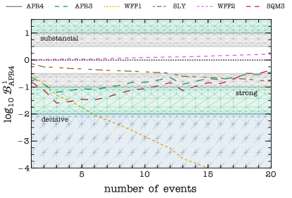
Figure 3: Evolution of the EoS Bayes factor with the number of events for the LIGO-Virgo network at design sensitivity. Top and bottom panels refer to the ALF2 (stiff EoS) and AP4 (soft EoS) injections, respectively. In each panel, the quantity $\log_{10}{\cal B}^{i}_{T}$ is normalized with respect to the injected EoS. Shaded bands mark the boundaries of the evidence criteria according to the Kass-Raftery scale [103]. In particular, $\log_{10}{\cal B}^{i}_{T}<-2$ indicates decisive unfavorable evidence.

The latter conclusion motivates to forecast a similar analysis in the era of third-generation GW detectors [76, 77, 78, 79, 80, 81, 82]. The situation here drastically changes, as shown in Fig. 4. We simulated the same 20 detections with ET, by assuming the conservative case of an underlying APR4 EoS, as in the bottom panel of Fig. 3. For each event, we plot the Bayes factors normalized by the injected EoS and we only show those EoS which have nonvanishing evidence ($\log_{10}{\cal B}_{\rm APR4}^{i}>-10$) for at least one event. The fact that most EoS have negligible evidence is a consequence of the much higher sensitivity of the ET detector, and it allows us to exclude all but a couple of EoS of our dataset (namely WFF2 and SLy, which feature a tidal deformability similar to APR4) with only a single observation.

Even in the most pessimistic case, in which a single observation is not enough to exclude a given EoS, stacking two/three detections would allow us to decisively exclude all EoS in the catalog other than the reference one. Even stronger conclusions apply to the case in which the reference EoS are stiff (as for ALF2): in this case all the other EoS in our catalog are decisively excluded for any single event.

Thus, at variance with advanced LIGO/Virgo, ET will be able to distinguish among EoS with similar softness, and also among EoS families featuring different microphysical properties (see Table 1). For example, a single ET detection of any of the $20$ events considered in our catalog would be sufficient to exclude APR3 relative to APR4 ($\log_{10}{\cal B}^{\rm APR3}_{\rm APR4}<-10$). These two EoS feature the same particle content but differ in the description of the nucleon interaction.

Conclusions. We proposed a robust Bayesian-ranking test to discriminate among families of ab-initio nuclear EoS using GW observations. We applied this test to GW170817, which very mildly favors a relatively soft, standard $npe\mu$ EoS (WFF2), although its power in ruling out EoS with similar stiffness is limited. Furthermore, we showed that near-future observations will not be conclusive: even $20$ NS binary detections with LIGO-Virgo at design sensitivity will not be able to distinguish among well-motivated nuclear models.

On the other hand, a single detection by ET will rule out with decisive statistical evidence most of the EoS, including those with comparable softness. In addition, just a few combined detections can be sufficient to robustly identify the best-fit EoS within a catalogue, hence constraining the particle content of nuclear matter at ultrahigh density. The same conclusion would apply assuming that binaries are observed by the proposed Cosmic Explorer [78, 79], which features a noise curve similar to that of ET-D at high frequencies, where tidal effects contribute more to the GW signal. Joint detections by ET and Cosmic Explorer would further strengthen our results.

Measuring the masses and tidal deformabilities from multiple events would allow us to quantify the faithfulness of the best-fit EoS, e.g. by looking for inconsistencies between the best-fit predictions and the data in the $\Lambda-M$ plane (see Fig. 1), in case the “true” EoS is not in the dataset.

A further advantage of our approach based on a ranking test among nuclear-physics based EoS is that it can be straightforwardly extended to accommodate other measurements by combining the likelihoods of different models. It would be interesting to extend our analysis in this direction by combining future GW observations with EM ones [51, 60], or with post-merger signals [26].

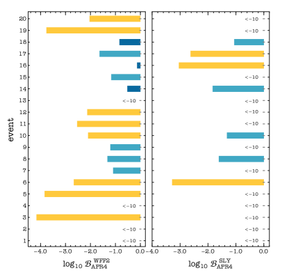
Figure 4: Bayes factors for simulated observations with ET, relative to the injected EoS APR4, for WFF2 and SLY. The remaining set of ten EoS yield $\log_{10}{\cal B}_{\rm APR4}^{i}<-10$ for all events, and they are not shown in the plot.

Acknowledgments. We are indebted to Swetha Bhagwat, Omar Benhar, Marica Branchesi, and Valeria Ferrari for discussions and comments on the manuscript. Numerical calculations have been made possible through a CINECA-INFN agreement, providing access to resources on MARCONI at CINECA. We acknowledge financial support provided under the European Union’s H2020 ERC, Starting Grant agreement no. DarkGRA–757480. We also acknowledge support under the MIUR PRIN and FARE programmes (GW-NEXT, CUP: B84I20000100001), and from the Amaldi Research Center funded by the MIUR program “Dipartimento di Eccellenza” (CUP: B81I18001170001).

Appendix. In Table 2 we list the masses and distances of the 20 binary NS sources considered in the main text. The masses were drawn uniformly in the range $(1.2,1.6)\,M_{\odot}$, whereas the luminosity distance $d_{L}$ was drawn uniformly in comoving volume with $60\leq d_{L}/{\rm Mpc}\leq 210$. For each event, we also show the 68% confidence intervals around the median for the tidal deformability inferred by projected LIGO-Virgo network and ET observations.

${\rm event}$	$m_{1}/M_{\odot}$	$m_{2}/M_{\odot}$	$d_{\textnormal{L}}/{\rm Mpc}$	$\tilde{\Lambda}_{\textnormal{APR4}}$	$\tilde{\Lambda}_{\textnormal{ALF2}}$	$\tilde{\Lambda}^{\textnormal{HLV}}_{\textnormal{APR4}}$	$\tilde{\Lambda}^{\textnormal{HLV}}_{\textnormal{ALF2}}$	$\tilde{\Lambda}^{\textnormal{ET}}_{\textnormal{APR4}}$
1	1.51	1.37	61	220	643	$221^{+71}_{-62}$	$627^{+79}_{-81}$	$220^{+4}_{-4}$
2	1.30	1.27	107	442	1200	$476^{+257}_{-159}$	$1132^{+217}_{-218}$	$441^{+8}_{-9}$
3	1.57	1.55	64	128	395	$138^{+53}_{-46}$	$386^{+62}_{-60}$	$127^{+3}_{-3}$
4	1.23	1.23	179	573	1510	$1085^{+880}_{-544}$	$1519^{+766}_{-532}$	$563^{+12}_{-12}$
5	1.48	1.25	165	313	873	$683^{+646}_{-351}$	$968^{+527}_{-329}$	$312^{+12}_{-9}$
6	1.54	1.28	132	257	730	$386^{+350}_{-169}$	$745^{+284}_{-204}$	$257^{+8}_{-8}$
7	1.47	1.40	167	223	655	$549^{+561}_{-302}$	$741^{+474}_{-264}$	$216^{+9}_{-9}$
8	1.48	1.36	182	240	697	$693^{+671}_{-391}$	$869^{+613}_{-345}$	$239^{+12}_{-13}$
9	1.33	1.33	204	359	1000	$1049^{+889}_{-573}$	$1247^{+826}_{-524}$	$349^{+13}_{-14}$
10	1.58	1.42	133	169	506	$275^{+274}_{-127}$	$518^{+220}_{-147}$	$168^{+7}_{-7}$
11	1.39	1.29	182	345	962	$809^{+729}_{-427}$	$1078^{+665}_{-394}$	$342^{+11}_{-12}$
12	1.35	1.31	191	359	1000	$925^{+836}_{-488}$	$1175^{+727}_{-457}$	$353^{+12}_{-12}$
13	1.34	1.25	112	424	1150	$463^{+287}_{-159}$	$1099^{+249}_{-233}$	$424^{+12}_{-12}$
14	1.41	1.40	208	255	739	$894^{+846}_{-504}$	$1024^{+770}_{-455}$	$243^{+12}_{-16}$
15	1.36	1.25	204	405	1110	$1106^{+894}_{-596}$	$1309^{+824}_{-532}$	$395^{+17}_{-16}$
16	1.49	1.46	130	187	558	$286^{+259}_{-132}$	$554^{+216}_{-149}$	$177^{+7}_{-8}$
17	1.57	1.31	186	225	648	$705^{+678}_{-396}$	$850^{+625}_{-351}$	$224^{+9}_{-9}$
18	1.54	1.45	198	171	515	$645^{+656}_{-374}$	$740^{+604}_{-325}$	$167^{+10}_{-10}$
19	1.33	1.22	153	466	1250	$733^{+616}_{-341}$	$1257^{+531}_{-385}$	$472^{+11}_{-12}$
20	1.44	1.29	205	309	870	$962^{+843}_{-539}$	$1134^{+803}_{-479}$	$312^{+10}_{-13}$

Table 2: Source parameters for the $20$ BNS considered in this work. The last three columns provide the $68\%$ confidence intervals around the median for the tidal deformability measured by the LIGO-Virgo network (HLV) and ET for each event.

References

- [1] F. Ozel, G. Baym, and T. Guver, “Astrophysical Measurement of the Equation of State of Neutron Star Matter,” Phys. Rev. D 82 (2010) 101301, arXiv:1002.3153 [astro-ph.HE].
- [2] J. M. Lattimer and M. Prakash, “Neutron Star Observations: Prognosis for Equation of State Constraints,” Phys. Rept. 442 (2007) 109–165, arXiv:astro-ph/0612440 [astro-ph].
- [3] F. Özel and P. Freire, “Masses, Radii, and the Equation of State of Neutron Stars,” Ann. Rev. Astron. Astrophys. 54 (2016) 401–440, arXiv:1603.02698 [astro-ph.HE].
- [4] E. Poisson and C. Will, Gravity: Newtonian, Post-Newtonian, Relativistic. Cambridge University Press, Cambridge, UK, 2014.
- [5] K. Chatziioannou, “Neutron star tidal deformability and equation of state constraints,” Gen. Rel. Grav. 52 no. 11, (2020) 109, arXiv:2006.03168 [gr-qc].
- [6] B.-A. Li and X. Han Phys. Lett. B 727 (2013) 276.
- [7] P. Russotto et al. Phys. Rev. C 94 (2016) 034608.
- [8] M. B. Tsang et al. Phys. Rev. Lett. 102 (2009) 122701.
- [9] P. Danielewicz and J. Lee Nucl. Phys. A 298 (2002) 1592.
- [10] B. A. Brown Phys. Rev. Lett. 922 (2014) 1.
- [11] Z. Zhang and L.-W. Chen Phys. Lett. B 726 (2013) 234 – 238.
- [12] P. Danielewicz, R. Lacey, and W. G. Lynch Science 298 (2002) 1592.
- [13] S. Shlomo, V. M. Kolomietz, and G. Colò The European Physical Journal A - Hadrons and Nuclei 30 no. 1, (2006) 23–30.
- [14] G. Colò Physics of Particles and Nuclei 39 no. 2, (2008) 286–305.
- [15] P. Demorest, T. Pennucci, S. Ransom, M. Roberts, and J. Hessels, “Shapiro Delay Measurement of A Two Solar Mass Neutron Star,” Nature 467 (2010) 1081–1083, arXiv:1010.5788 [astro-ph.HE].
- [16] J. Antoniadis et al., “A Massive Pulsar in a Compact Relativistic Binary,” Science 340 (2013) 6131, arXiv:1304.6875 [astro-ph.HE].
- [17] E. Fonseca et al., “The NANOGrav Nine-year Data Set: Mass and Geometric Measurements of Binary Millisecond Pulsars,” Astrophys. J. 832 no. 2, (2016) 167, arXiv:1603.00545 [astro-ph.HE].
- [18] H. T. Cromartie et al., “Relativistic Shapiro delay measurements of an extremely massive millisecond pulsar,” Nature Astron. 4 no. 1, (2019) 72–76, arXiv:1904.06759 [astro-ph.HE].
- [19] A. W. Steiner, J. M. Lattimer, and E. F. Brown, “The Equation of State from Observed Masses and Radii of Neutron Stars,” Astrophys. J. 722 (2010) 33–54, arXiv:1005.0811 [astro-ph.HE].
- [20] T. Guver and F. Ozel, “The mass and the radius of the neutron star in the transient low mass X-ray binary SAX J1748.9-2021,” Astrophys. J. Lett. 765 (2013) L1, arXiv:1301.0831 [astro-ph.HE].
- [21] T. E. Riley et al., “A View of PSR J0030+0451: Millisecond Pulsar Parameter Estimation,” Astrophys. J. Lett. 887 no. 1, (2019) L21, arXiv:1912.05702 [astro-ph.HE].
- [22] M. Miller et al., “PSR J0030+0451 Mass and Radius from Data and Implications for the Properties of Neutron Star Matter,” Astrophys. J. Lett. 887 no. 1, (2019) L24, arXiv:1912.05705 [astro-ph.HE].
- [23] LIGO Scientific, Virgo Collaboration, B. Abbott et al., “Gw170817: Observation of gravitational waves from a binary neutron star inspiral,” Phys. Rev. Lett. 119 no. 16, (2017) 161101, arXiv:1710.05832 [gr-qc].
- [24] LIGO Scientific, Virgo Collaboration, B. Abbott et al., “Properties of the binary neutron star merger GW170817,” Phys. Rev. X 9 no. 1, (2019) 011001, arXiv:1805.11579 [gr-qc].
- [25] LIGO Scientific, Virgo Collaboration, B. Abbott et al., “GW190425: Observation of a Compact Binary Coalescence with Total Mass ,” Astrophys. J. Lett. 892 no. 1, (2020) L3, arXiv:2001.01761 [astro-ph.HE].
- [26] L. Baiotti and L. Rezzolla, “Binary neutron star mergers: a review of Einstein’s richest laboratory,” Rept. Prog. Phys. 80 no. 9, (2017) 096901, arXiv:1607.03540 [gr-qc].
- [27] E. E. Flanagan and T. Hinderer, “Constraining neutron star tidal Love numbers with gravitational wave detectors,” Phys. Rev. D 77 (2008) 021502, arXiv:0709.1915 [astro-ph].
- [28] T. Hinderer, “Tidal Love numbers of neutron stars,” Astrophys. J. 677 (2008) 1216–1220, arXiv:0711.2420 [astro-ph].
- [29] T. Hinderer, B. D. Lackey, R. N. Lang, and J. S. Read, “Tidal deformability of neutron stars with realistic equations of state and their gravitational wave signatures in binary inspiral,” Physical Review D 81 no. 12, (June, 2010) 101–12.
- [30] L. Baiotti, T. Damour, B. Giacomazzo, A. Nagar, and L. Rezzolla, “Analytic modelling of tidal effects in the relativistic inspiral of binary neutron stars,” Phys.Rev.Lett. 105 (2010) 261101, arXiv:1009.0521 [gr-qc].
- [31] L. Baiotti, T. Damour, B. Giacomazzo, A. Nagar, and L. Rezzolla, “Accurate numerical simulations of inspiralling binary neutron stars and their comparison with effective-one-body analytical models,” Phys.Rev. D84 (2011) 024017, arXiv:1103.3874 [gr-qc].
- [32] J. Vines, E. E. Flanagan, and T. Hinderer, “Post-1-Newtonian tidal effects in the gravitational waveform from binary inspirals,” Phys. Rev. D 83 (2011) 084051, arXiv:1101.1673 [gr-qc].
- [33] F. Pannarale, L. Rezzolla, F. Ohme, and J. S. Read, “Will black hole-neutron star binary inspirals tell us about the neutron star equation of state?,” Phys.Rev. D84 (2011) 104017, arXiv:1103.3526 [astro-ph.HE].
- [34] J. E. Vines and E. E. Flanagan, “Post-1-Newtonian quadrupole tidal interactions in binary systems,” Phys. Rev. D 88 (2013) 024046, arXiv:1009.4919 [gr-qc].
- [35] B. D. Lackey, K. Kyutoku, M. Shibata, P. R. Brady, and J. L. Friedman, “Extracting equation of state parameters from black hole-neutron star mergers. I. Nonspinning black holes,” Phys.Rev. D85 (2012) 044061, arXiv:1109.3402 [astro-ph.HE].
- [36] A. Maselli, L. Gualtieri, and V. Ferrari, “Constraining the equation of state of nuclear matter with gravitational wave observations: Tidal deformability and tidal disruption,” Phys. Rev. D88 no. 10, (2013) 104040, arXiv:1310.5381 [gr-qc].
- [37] B. D. Lackey, K. Kyutoku, M. Shibata, P. R. Brady, and J. L. Friedman, “Extracting equation of state parameters from black hole-neutron star mergers: aligned-spin black holes and a preliminary waveform model,” Phys.Rev. D89 no. 4, (2014) 043009, arXiv:1303.6298 [gr-qc].
- [38] M. Favata, “Systematic parameter errors in inspiraling neutron star binaries,” Phys. Rev. Lett. 112 (2014) 101101, arXiv:1310.8288 [gr-qc].
- [39] W. Del Pozzo, T. G. F. Li, M. Agathos, C. Van Den Broeck, and S. Vitale, “Demonstrating the feasibility of probing the neutron star equation of state with second-generation gravitational wave detectors,” Phys. Rev. Lett. 111 no. 7, (2013) 071101, arXiv:1307.8338 [gr-qc].
- [40] B. D. Lackey and L. Wade, “Reconstructing the neutron-star equation of state with gravitational-wave detectors from a realistic population of inspiralling binary neutron stars,” Phys. Rev. D 91 no. 4, (2015) 043002, arXiv:1410.8866 [gr-qc].
- [41] A. Guerra Chaves and T. Hinderer, “Probing the equation of state of neutron star matter with gravitational waves from binary inspirals in light of GW170817: a brief review,” J. Phys. G 46 no. 12, (2019) 123002, arXiv:1912.01461 [nucl-th].
- [42] E. Annala, T. Gorda, A. Kurkela, and A. Vuorinen, “Gravitational-wave constraints on the neutron-star-matter Equation of State,” Phys. Rev. Lett. 120 no. 17, (2018) 172703, arXiv:1711.02644 [astro-ph.HE].
- [43] B. Margalit and B. D. Metzger, “Constraining the Maximum Mass of Neutron Stars From Multi-Messenger Observations of GW170817,” Astrophys. J. Lett. 850 no. 2, (2017) L19, arXiv:1710.05938 [astro-ph.HE].
- [44] D. Radice, A. Perego, F. Zappa, and S. Bernuzzi, “GW170817: Joint Constraint on the Neutron Star Equation of State from Multimessenger Observations,” Astrophys. J. Lett. 852 no. 2, (2018) L29, arXiv:1711.03647 [astro-ph.HE].
- [45] A. Bauswein, O. Just, H.-T. Janka, and N. Stergioulas, “Neutron-star radius constraints from GW170817 and future detections,” Astrophys. J. Lett. 850 no. 2, (2017) L34, arXiv:1710.06843 [astro-ph.HE].
- [46] Y. Lim and J. W. Holt, “Neutron star tidal deformabilities constrained by nuclear theory and experiment,” Phys. Rev. Lett. 121 no. 6, (2018) 062701, arXiv:1803.02803 [nucl-th].
- [47] E. R. Most, L. R. Weih, L. Rezzolla, and J. Schaffner-Bielich, “New constraints on radii and tidal deformabilities of neutron stars from GW170817,” Phys. Rev. Lett. 120 no. 26, (2018) 261103, arXiv:1803.00549 [gr-qc].
- [48] Z. Carson, A. W. Steiner, and K. Yagi, “Constraining nuclear matter parameters with GW170817,” Phys. Rev. D 99 no. 4, (2019) 043010, arXiv:1812.08910 [gr-qc].
- [49] S. De, D. Finstad, J. M. Lattimer, D. A. Brown, E. Berger, and C. M. Biwer, “Tidal Deformabilities and Radii of Neutron Stars from the Observation of GW170817,” Phys. Rev. Lett. 121 no. 9, (2018) 091102, arXiv:1804.08583 [astro-ph.HE]. [Erratum: Phys.Rev.Lett. 121, 259902 (2018)].
- [50] E. Annala, T. Gorda, A. Kurkela, J. Nättilä, and A. Vuorinen, “Evidence for quark-matter cores in massive neutron stars,” Nature Phys. (2020) , arXiv:1903.09121 [astro-ph.HE].
- [51] G. Raaijmakers et al., “Constraining the dense matter equation of state with joint analysis of NICER and LIGO/Virgo measurements,” Astrophys. J. Lett. 893 no. 1, (2020) L21, arXiv:1912.11031 [astro-ph.HE].
- [52] C. D. Capano, I. Tews, S. M. Brown, B. Margalit, S. De, S. Kumar, D. A. Brown, B. Krishnan, and S. Reddy, “Stringent constraints on neutron-star radii from multimessenger observations and nuclear theory,” Nature Astron. 4 no. 6, (2020) 625–632, arXiv:1908.10352 [astro-ph.HE].
- [53] M. C. Miller, C. Chirenti, and F. K. Lamb, “Constraining the equation of state of high-density cold matter using nuclear and astronomical measurements,” arXiv:1904.08907 [astro-ph.HE].
- [54] B. Kumar and P. Landry, “Inferring neutron star properties from GW170817 with universal relations,” Phys. Rev. D 99 no. 12, (2019) 123026, arXiv:1902.04557 [gr-qc].
- [55] M. Fasano, T. Abdelsalhin, A. Maselli, and V. Ferrari, “Constraining the Neutron Star Equation of State Using Multiband Independent Measurements of Radii and Tidal Deformabilities,” Phys. Rev. Lett. 123 no. 14, (2019) 141101, arXiv:1902.05078 [astro-ph.HE].
- [56] H. Güven, K. Bozkurt, E. Khan, and J. Margueron, “Multi-messenger and multi-physics Bayesian inference for GW170817 binary neutron star merger,” Phys. Rev. C 102 no. 1, (2020) 015805, arXiv:2001.10259 [nucl-th].
- [57] S. Traversi, P. Char, and G. Pagliara, “Bayesian Inference of Dense Matter Equation of State within Relativistic Mean Field Models using Astrophysical Measurements,” Astrophys. J. 897 (2020) 165, arXiv:2002.08951 [astro-ph.HE].
- [58] P. Landry, R. Essick, and K. Chatziioannou, “Nonparametric constraints on neutron star matter with existing and upcoming gravitational wave and pulsar observations,” Phys. Rev. D 101 no. 12, (2020) 123007, arXiv:2003.04880 [astro-ph.HE].
- [59] T. Dietrich, M. W. Coughlin, P. T. H. Pang, M. Bulla, J. Heinzel, L. Issa, I. Tews, and S. Antier, “Multimessenger constraints on the neutron-star equation of state and the Hubble constant,” Science 370 no. 6523, (2020) 1450–1453, arXiv:2002.11355 [astro-ph.HE].
- [60] J. Zimmerman, Z. Carson, K. Schumacher, A. W. Steiner, and K. Yagi, “Measuring Nuclear Matter Parameters with NICER and LIGO/Virgo,” arXiv:2002.03210 [astro-ph.HE].
- [61] H. O. Silva, A. M. Holgado, A. Cárdenas-Avendaño, and N. Yunes, “Astrophysical and theoretical physics implications from multimessenger neutron star observations,” arXiv:2004.01253 [gr-qc].
- [62] M. Al-Mamun, A. W. Steiner, J. Nättilä, J. Lange, R. O’Shaughnessy, I. Tews, S. Gandolfi, C. Heinke, and S. Han, “Combining Electromagnetic and Gravitational-Wave Constraints on Neutron-Star Masses and Radii,” Phys. Rev. Lett. 126 no. 6, (2021) 061101, arXiv:2008.12817 [astro-ph.HE].
- [63] A. Sabatucci and O. Benhar, “Tidal deformation of neutron stars from microscopic models of nuclear dynamics,” Phys. Rev. C 1091 (2020) 0545807.
- [64] A. Maselli, A. Sabatucci, and O. Benhar, “Constraining three-nucleon forces with multimessenger data,” arXiv:2010.03581 [astro-ph.HE].
- [65] L. Baiotti, “Gravitational waves from neutron star mergers and their relation to the nuclear equation of state,” Prog. Part. Nucl. Phys. 109 no. 12, (2019) 103714.
- [66] J. S. Read, B. D. Lackey, B. J. Owen, and J. L. Friedman, “Constraints on a phenomenologically parameterized neutron-star equation of state,” Phys. Rev. D 79 (2009) 124032, arXiv:0812.2163 [astro-ph].
- [67] L. Lindblom, “Spectral Representations of Neutron-Star Equations of State,” Phys. Rev. D 82 (2010) 103011, arXiv:1009.0738 [astro-ph.HE].
- [68] K. Hebeler, J. M. Lattimer, C. J. Pethick, and A. Schwenk, “Equation of state and neutron star properties constrained by nuclear physics and observation,” Astrophys. J. 773 (2013) 11, arXiv:1303.4662 [astro-ph.SR].
- [69] S. K. Greif, G. Raaijmakers, K. Hebeler, A. Schwenk, and A. L. Watts, “Equation of state sensitivities when inferring neutron star and dense matter properties,” Mon. Not. Roy. Astron. Soc. 485 no. 4, (2019) 5363–5376, arXiv:1812.08188 [astro-ph.HE].
- [70] K. Hebeler, J. D. Holt, J. Menendez, and A. Schwenk, “Nuclear forces and their impact on neutron-rich nuclei and neutron-rich matter,” Ann. Rev. Nucl. Part. Sci. 65 (2015) 457–484, arXiv:1508.06893 [nucl-th].
- [71] I. Tews, J. Carlson, S. Gandolfi, and S. Reddy, “Constraining the speed of sound inside neutron stars with chiral effective field theory interactions and observations,” Astrophys. J. 860 no. 2, (2018) 149, arXiv:1801.01923 [nucl-th].
- [72] B. Biswas, P. Char, R. Nandi, and S. Bose, “Towards mitigation of apparent tension between nuclear physics and astrophysical observations by improved modeling of neutron star matter,” Phys. Rev. D 103 no. 10, (2021) 103015, arXiv:2008.01582 [astro-ph.HE].
- [73] P. Landry and R. Essick, “Nonparametric inference of the neutron star equation of state from gravitational wave observations,” Phys. Rev. D 99 no. 8, (2019) 084049, arXiv:1811.12529 [gr-qc].
- [74] E. Fonseca et al., “Refined Mass and Geometric Measurements of the High-Mass PSR J0740+6620,” arXiv:2104.00880 [astro-ph.HE].
- [75] LIGO Scientific, Virgo Collaboration, B. P. Abbott et al., “Model comparison from LIGO–Virgo data on GW170817’s binary components and consequences for the merger remnant,” Class. Quant. Grav. 37 no. 4, (2020) 045006, arXiv:1908.01012 [gr-qc].
- [76] M. Punturo et al., “The Einstein Telescope: A third-generation gravitational wave observatory,” Class. Quant. Grav. 27 (2010) 194002.
- [77] S. Dwyer, D. Sigg, S. W. Ballmer, L. Barsotti, N. Mavalvala, and M. Evans, “Gravitational wave detector with cosmological reach,” Phys. Rev. D 91 (Apr, 2015) 082001. https://link.aps.org/doi/10.1103/PhysRevD.91.082001.
- [78] LIGO Scientific Collaboration, B. P. Abbott et al., “Exploring the Sensitivity of Next Generation Gravitational Wave Detectors,” Class. Quant. Grav. 34 no. 4, (2017) 044001, arXiv:1607.08697 [astro-ph.IM].
- [79] R. Essick, S. Vitale, and M. Evans, “Frequency-dependent responses in third generation gravitational-wave detectors,” Phys. Rev. D96 no. 8, (2017) 084004, arXiv:1708.06843 [gr-qc].
- [80] S. Hild et al., “Sensitivity Studies for Third-Generation Gravitational Wave Observatories,” Class. Quant. Grav. 28 (2011) 094013, arXiv:1012.0908 [gr-qc].
- [81] B. S. Sathyaprakash et al., “Extreme Gravity and Fundamental Physics,” arXiv:1903.09221 [astro-ph.HE].
- [82] M. Maggiore et al., “Science Case for the Einstein Telescope,” JCAP 03 (2020) 050, arXiv:1912.02622 [astro-ph.CO].
- [83] A. Akmal, V. Pandharipande, and D. Ravenhall, “The Equation of state of nucleon matter and neutron star structure,” Phys. Rev. C 58 (1998) 1804–1828, arXiv:nucl-th/9804027.
- [84] F. Douchin and P. Haensel, “A unified equation of state of dense matter and neutron star structure,” Astron. Astrophys. 380 (2001) 151, arXiv:astro-ph/0111092.
- [85] H. Müther, M. Prakash, and T. Ainsworth, “The nuclear symmetry energy in relativistic Brueckner-Hartree-Fock calculations,” Phys. Lett. B 199 (1987) 469–474.
- [86] H. Mueller and B. D. Serot, “Relativistic mean field theory and the high density nuclear equation of state,” Nucl. Phys. A606 (1996) 508–537, arXiv:nucl-th/9603037 [nucl-th].
- [87] R. B. Wiringa, V. Fiks, and A. Fabrocini, “Equation of state for dense nucleon matter,” Phys. Rev. C 38 (1988) 1010–1037.
- [88] N. Glendenning, “Neutron Stars Are Giant Hypernuclei?,” Astrophys. J. 293 (1985) 470–493.
- [89] B. D. Lackey, M. Nayyar, and B. J. Owen, “Observational constraints on hyperons in neutron stars,” Phys. Rev. D 73 (2006) 024021, arXiv:astro-ph/0507312.
- [90] M. Alford, M. Braby, M. Paris, and S. Reddy, “Hybrid stars that masquerade as neutron stars,” Astrophys. J. 629 (2005) 969–978, arXiv:nucl-th/0411016.
- [91] M. Prakash, J. Cooke, and J. Lattimer, “Quark - hadron phase transition in protoneutron stars,” Phys. Rev. D 52 (1995) 661–665.
- [92] J. M. Lattimer and M. Prakash, “Neutron star structure and the equation of state,” Astrophys. J. 550 (2001) 426, arXiv:astro-ph/0002232.
- [93] O. Benhar and S. Fantoni, Nuclear Matter Theory. CRC Press, 2020. https://books.google.it/books?id=UFDhDwAAQBAJ.
- [94] M. Mapelli and N. Giacobbo, “The cosmic merger rate of neutron stars and black holes,” Mon. Not. Roy. Astron. Soc. 479 no. 4, (2018) 4391–4398, arXiv:1806.04866 [astro-ph.HE].
- [95] T. Dietrich, S. Bernuzzi, and W. Tichy, “Closed-form tidal approximants for binary neutron star gravitational waveforms constructed from high-resolution numerical relativity simulations,” Phys. Rev. D 96 no. 12, (2017) 121501, arXiv:1706.02969 [gr-qc].
- [96] T. Dietrich et al., “Matter imprints in waveform models for neutron star binaries: Tidal and self-spin effects,” Phys. Rev. D 99 no. 2, (2019) 024029, arXiv:1804.02235 [gr-qc].
- [97] L. Wade, J. D. E. Creighton, E. Ochsner, B. D. Lackey, B. F. Farr, T. B. Littenberg, and V. Raymond, “Systematic and statistical errors in a bayesian approach to the estimation of the neutron-star equation of state using advanced gravitational wave detectors,” Phys. Rev. D89 no. 10, (2014) 103012, arXiv:1402.5156 [gr-qc].
- [98] M. Pitkin, S. Reid, S. Rowan, and J. Hough, “Gravitational Wave Detection by Interferometry (Ground and Space),” Living Rev. Rel. 14 (2011) 5, arXiv:1102.3355 [astro-ph.IM].
- [99] G. Ashton et al., “BILBY: A user-friendly Bayesian inference library for gravitational-wave astronomy,” Astrophys. J. Suppl. 241 no. 2, (2019) 27, arXiv:1811.02042 [astro-ph.IM].
- [100] I. M. Romero-Shaw et al., “Bayesian inference for compact binary coalescences with bilby: validation and application to the first LIGO–Virgo gravitational-wave transient catalogue,” Mon. Not. Roy. Astron. Soc. 499 no. 3, (2020) 3295–3319, arXiv:2006.00714 [astro-ph.IM].
- [101] S. A. Usman, J. C. Mills, and S. Fairhurst, “Constraining the Inclinations of Binary Mergers from Gravitational-wave Observations,” Astrophys. J. 877 no. 2, (2019) 82, arXiv:1809.10727 [gr-qc].
- [102] H.-Y. Chen, S. Vitale, and R. Narayan, “Viewing angle of binary neutron star mergers,” Phys. Rev. X 9 no. 3, (2019) 031028, arXiv:1807.05226 [astro-ph.HE].
- [103] R. E. Kass and A. E. Raftery, “Bayes factors,” Journal of the american statistical association 90 no. 430, (1995) 773–795.
- [104] LIGO Scientific, Virgo Collaboration, B. P. Abbott et al., “GWTC-1: A Gravitational-Wave Transient Catalog of Compact Binary Mergers Observed by LIGO and Virgo during the First and Second Observing Runs,” Phys. Rev. X 9 no. 3, (2019) 031040, arXiv:1811.12907 [astro-ph.HE].
- [105] LIGO Scientific, Virgo Collaboration, R. Abbott et al., “GWTC-2: Compact Binary Coalescences Observed by LIGO and Virgo During the First Half of the Third Observing Run,” arXiv:2010.14527 [gr-qc].
- [106] LIGO Scientific, Virgo Collaboration, B. P. Abbott et al., “GW170817: Measurements of neutron star radii and equation of state,” Phys. Rev. Lett. 121 no. 16, (2018) 161101, arXiv:1805.11581 [gr-qc].
- [107] I. Harry and T. Hinderer, “Observing and measuring the neutron-star equation-of-state in spinning binary neutron star systems,” Class. Quant. Grav. 35 no. 14, (2018) 145010, arXiv:1801.09972 [gr-qc].