Review of end-to-end speech synthesis technology based on deep learning

Abstract

As an indispensable part of modern human-computer interaction system, speech synthesis technology helps users get the output of intelligent machine more easily and intuitively, thus has attracted more and more attention. Due to the limitations of high complexity and low efficiency of traditional speech synthesis technology, the current research focus is the deep learning-based end-to-end speech synthesis technology, which has more powerful modeling ability and a simpler pipeline. It mainly consists of three modules: text front-end, acoustic model, and vocoder. This paper reviews the research status of these three parts, and classifies and compares various methods according to their emphasis. Moreover, this paper also summarizes the open-source speech corpus of English, Chinese and other languages that can be used for speech synthesis tasks, and introduces some commonly used subjective and objective speech quality evaluation method. Finally, some attractive future research directions are pointed out.

1 Introduction

With the rapid development of computer science, artificial intelligence, automation and robot control technology, the demand of human-computer interaction has been fully met and the way has become more and more direct and convenient. Human-computer interaction relies heavily on speech communication. The speech system of the machine is divided into three functional modules: voiceprint recognition, speech recognition and speech synthesis. The most difficult and complex task is speech synthesis. This is because that compared to speech and voiceprint recognition, speech synthesis systems usually require more data for training and more complex models for modeling in order to accurately synthesize high-fidelity speech with various styles by inputting simple text.

Speech synthesis is also called text-to-speech (TTS) when the input is text. TTS is a frontier technology in the field of information processing, which involves many disciplines such as acoustics, linguistics, and computer science. The main task is to convert input text into output speech. TTS system is the mouth of the intelligent machine, which has been widely used in various fields of people’s daily life, such as voice navigation, information broadcast, intelligent assistant, intelligent customer service, and has achieved great economic benefits. Moreover, it is also being applied to some new fields, such as article reading, language education, video dubbing, and rehabilitation therapy. TTS applications has become an important part of people’s lives.

Deep learning-based TTS technology

With the development of computer science and technology, the intelligibility and naturalness of synthesized speech have been greatly improved due to the continuous improvement of TTS techniques from the formant-based methods Vogten and Berendsen (1988); Klatt (1987); Kang and Hong (2011); Khorinphan et al. (2014); Klatt (1980); Schröder (2001) to the unit selection-based waveform cascade methods Capes et al. (2017); Chu et al. (2003); Murray et al. (1996); Moulines and Charpentier (1990); Atal and Hanauer (1971); Hunt and Black (1996); Gonzalvo et al. (2016), and to the hidden Markov model (HMM)-based statistical parametric speech synthesis (SPSS) methods Saito et al. (2017); Chen et al. (2015); Nose (2016); Tokuda et al. (2013); Kawahara et al. (2008); Yoshimura et al. (1999); Zen et al. (2007, 2009). Deep learning is a new research direction in the field of artificial intelligence in recent years. This method can effectively capture the latent information and association in data, and has more powerful modeling ability than traditional statistical learning methods Yang et al. (2014). TTS methods based on deep learning have been widely researched Ze et al. (2013); Fernandez et al. (2013); Lu et al. (2013); Qian et al. (2014). For example, in the SPSS model based on deep neural network (DNN), DNN can learn the mapping function from linguistic features (input) to acoustic features (output).

DNN-based acoustic models provide an effective distributed representation of the complex dependencies between linguistic features and acoustic features. However, one limitation of the acoustic feature modeling method based on feedforward DNN is that it ignores the continuity of speech. The DNN-based method assumes that each frame is sampled independently, although there is correlation between consecutive frames in the speech data. Recurrent Neural Network (RNN) provides an effective method to model the correlation between adjacent frames of speech, because it can use all the available input features to predict the output features of each frame. Based on this, some researchers use RNN instead of DNN to capture the long-term dependence of speech frames in order to improve the quality of synthesized speech Zen and Sak (2015); Tuerk and Robinson (1993); Karaali et al. (1998); Fan et al. (2014); Fernandez et al. (2014); Zen et al. (2014).

End-to-end TTS technology

The traditional SPSS network is a complex pipeline containing many modules, composed of text-to-phoneme network, audio segmentation network, phoneme duration prediction network, fundamental frequency prediction network and vocoder Arık et al. (2017); Gibiansky et al. (2017). Building these modules requires a lot of professional knowledge and complex engineering implementation, which will take a lot of time and effort. Also, the combination of errors in each component may make the model difficult to train. End-to-end TTS methods are driven by the desire to simplify TTS systems and reduce the need for manual intervention and linguistic background knowledge. The end-to-end TTS model only needs to be trained from scratch on the paired data set of $\langle$text, speech$\rangle$, and can directly synthesize speech from the text. The state-of-the-art end-to-end TTS models based on deep learning have been able to synthesize speech close to human voice Wang et al. (2017); Shen et al. (2018); Oord et al. (2016).

It is mainly composed of three parts: text analysis front-end, acoustic model and vocoder, as shown in Fig. 1. Firstly, the text front-end converts the text into standard input. Then, the acoustic model converts the standard input into intermediate acoustic features, which are used to model the long-term structure of speech. The most common intermediate acoustic features are spectrogram Wang et al. (2017); Shen et al. (2018), vocoder feature Sotelo et al. (2017) or linguistic feature Oord et al. (2016). Finally, the vocoder is used to fill in low-level signal details and convert acoustic features into time-domain waveform samples. To reduce the difficulty of training and improve the quality of synthesized speech, the text front-end, acoustic model and vocoder are usually trained separately Shen et al. (2018), and they can also be fine-tuned jointly Sotelo et al. (2017). This article will introduce some of the latest developments in each of the three components according to the structure of Fig. 2.

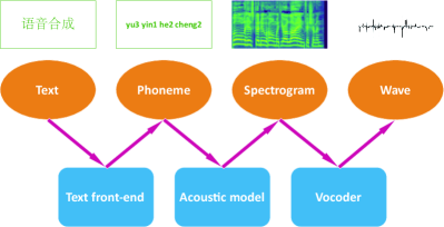
Figure 1: Pipeline architecture for TTS

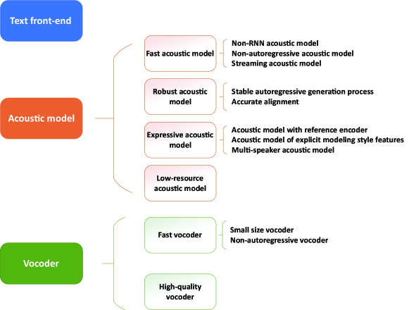
Figure 2: Section organization of the TTS model

There have been some reviews on TTS. For example, Deng et al. (2018) analyzed the number of documents and citations of TTS papers from 1992 to 2017, aiming to help researchers understand the development trend of TTS. Aroon and Dhonde (2015) reviewed SPSS methods based on HMM. Adiga and Prasanna (2019) reviewed SPSS methods and partially deep learning based methods. Ning et al. (2019) and Sruthi and Meharban (2020) reviewed TTS methods based on deep learning. Kalita and Deb (2017) reviewed emotional TTS methods for Hindi. Tits et al. (2019) reviewed the emotional speech corpus that could be used for TTS.

Although there have been some reviews on TTS methods based on deep learning, only some of baseline models have been introduced, such as WaveNet Oord et al. (2016), Tacotron Wang et al. (2017) and SampleRNN Mehri et al. (2016). These models have many problems, such as slow training and inference speed, instability, lack of emotion and rhythm in synthesized speech, and a large amount of high-quality speech data required for training. The state-of-the-art TTS methods can completely or partially solve these problems, still so far there has been no comprehensive review of the latest deep learning-based TTS models. Moreover, the quantity and quality of training speech corpus play a decisive role in the training results of TTS model, and how to effectively evaluate the quality of synthesized speech has always been a problem in the field of TTS. Therefore, this paper will make a detailed summary of the latest end-to-end TTS models based on deep learning, speech corpus and evaluation methods of synthesized speech, and finally give some future research directions.

The rest of this paper is organized as follows: Sect. 2, 3 and 4 respectively introduce the latest text front-end, acoustic model and vocoder based on deep learning. Sect. 5 organizes the corpus that could be used for TTS. Sect. 6 introduces commonly used synthesized speech evaluation methods from both subjective and objective aspects. Sect. 7 puts forward some challenges and future research directions for reference. The last section draws a general conclusion of this paper.

2 Text front-end

It is difficult to synthesize high-fidelity speech only using original phonemes or original text as the input of the TTS model, especially for languages that contain polyphonic characters and have complex prosodic structures, such as Mandarin. Therefore, it is necessary to use the text front-end to introduce additional pronunciation and syntactic information. The text front-end predicts the pronunciation mode from the original text, aiming to provide enough information for the back-end to accurately synthesize speech. The quality of the text front-end has a great impact on the clarity and naturalness of the synthesized speech. Pronunciation patterns are important information for languages with many polyphonic characters and ambiguous pronunciations, such as Mandarin. Syntactic information also contributes a lot to the pronunciation of a sentence, which determines the pause and tone of a sentence. People usually read a phrase that has a full meaning in its entirety, and pause between phrases that need to be separated. For languages with many ambiguities, the effect of syntactic information on sentence segmentation may also cause listeners to have a completely different understanding of a sentence. Therefore, this information needs to be predicted by the text front-end as a conditional input of the acoustic model to synthesize speech with correct pronunciation and prosody.

The traditional Mandarin text front-end is a cascade system, which consists of a series of text processing components, such as text normalization (TN), Chinese word segmentation (CWS), part-of-speech (POS) tagging, grapheme-to-phoneme (G2P) and prosodic structure prediction (PSP). The text front-end structure of other languages is similar to that of Mandarin. These components are usually modeled by traditional statistical methods, such as syntactic trees Zhang et al. (2016) and CRF Qian et al. (2010) based methods for PSP tasks and dictionary matching based methods Huang et al. (2010) for pronunciation prediction tasks. However, these traditional text front-ends often fail to predict correctly in some unusual or complex contexts. To boost prediction accuracy, some researchers have adopted state-of-the-art NLP frameworks based on deep learning methods such as BLSTM-CRF Zheng et al. (2018); Huang et al. (2015), Word2Vec Mikolov et al. (2013), Transformer Vaswani et al. (2017) and BERT Devlin et al. (2018) to improve the text front-end model based on dictionary and traditional statistical learning methods. These models can extract contextual information from the text effectively, and thus help the text front-end to accurately determine the pronunciation of polyphonic characters, the meaning of ambiguous sentences, and the prosodic boundaries between each word, each phrase and each sentence. The following will introduce the latest text front-end model based on deep learning from the aspects of text normalization, prosodic structure prediction, pronunciation prediction, contextual information extraction and so on.

Text normalization

Text normalization is an important preprocessing step for TTS tasks. Zhang et al. (2020a) standardized Mandarin text by combining the traditional rule-based system with a neural text network consisting of multi-head self-attention modules in Transformer to convert Non-Standard Words (NSW) into Spoken-Form Words (SFW). This method has a higher prediction accuracy than the rule-based system.

Prosodic structure prediction

Prosodic structure prediction is also an important function of the text front-end. Taking Mandarin as an example, the prosodic structure of Mandarin is a three-level hierarchical structure composed of three basic units: prosodic words (PW), prosodic phrases (PPH) and intonation phrases (IPH) Chu and Qian (2001). Because these three levels of prediction tasks are interrelated, Pan et al. (2019) modeled prosody information at all levels of the text in the way of multi-task learning, and proposed a Mandarin prosodic boundary prediction model based on BLSTM-CRF, which improved the prediction accuracy and simplified the model. Lu et al. (2019) also proposed a method of multi-tasking learning to efficiently complete PSP tasks based on the self-attention model.

Pronunciation prediction

Other text front-ends have the pronunciation prediction function on the basis of text normalization and prosody prediction. The G2P tasks of Mandarin can be divided into two categories: G2P of monophonic characters and G2P of polyphonic characters. The pronunciation of monophonic characters can be easily determined by a pronunciation dictionary, while G2P of polyphonic characters is highly context sensitive Zhang et al. (2020b). Therefore, disambiguation of polyphonic characters is the main task of Mandarin G2P. To accurately predict the pronunciation of polyphonic characters, Cai et al. (2019), Shan et al. (2016) and Park and Lee (2020) proposed to use Bi-LSTM network for G2P. On the basis of Pan et al. (2019), Yang et al. (2019) proposed to preprocess the original text by replacing the Word2Vec model with the encoder of Transformer-based NLP model and BERT pre-training model, and then carry out G2P and PSP in the Mandarin text front-end. The accuracy of prediction can be improved by taking advantage of Transformer and BERT network. However, pre-training models, such as BERT, are too large to be used in realtime applications and edge devices. To reduce the size of the model, Zhang et al. (2020b) proposed to use the simplified TinyBERT model Jiao et al. (2019) for the G2P and PSP tasks simultaneously using multi-task learning. It can ensure the accuracy of the prediction results while reducing the size of the model. Conkie and Finch (2020) proposed a text front-end that can be used to process multiple languages, including text normalization and G2P functions. They regard these two front-end tasks as two neural machine translation (NMT) tasks and use Transformer for modeling. Byte pair encoding (BPE) technology Sennrich et al. (2015) is also used to process uncommon words, and the splicing technique is used for long texts, which improves the accuracy of prediction and the quality of synthesized speech.

Introduction of style information

The text front-end can also directly add additional style information to the TTS system to provide the synthesized speech style features. For example, Tahon et al. (2018) added a pronunciation adaptive framework based on CRF between text front-end and TTS model to generate different styles of speech. In order to make the synthesized speech closer to human voice, Székely et al. (2020) took the front and back utterances of an utterance and the breath pronunciation events between them as a data set to learn the breath location information of the context, thus adding human breath information into the training data. The forward and backward breath predictors were also used to predict the location of breath more accurately.

Contextual information extraction

The text front-end model can also extract the contextual information of the text. The extracted additional contextual information can be input into the acoustic model as prior knowledge. For example, Hayashi et al. (2019) directly used BERT as a context feature extraction network to encode input text, and added encoded word or sentence-level contextual information to the input of the encoder of the acoustic model to improve the quality of synthesized speech. In order to obtain the phrase structure of the sentence and word relationship information, Guo et al. (2019a) used the factor parser Klein et al. (2003) in the Stanford parser to extract the syntactic tree. Then, the embedding vectors of extracted syntactic features and input tokens are then combined as the input of the acoustic model encoder, enabling TTS models to correctly synthesize speech when facing some ambiguous sentences. In order to improve the quality of synthesized speech, GraphSpeech Liu et al. (2020a) inputs syntactic knowledge as additional contextual information into the self-attention module of Transformer-TTS Li et al. (2019). The syntax tree of the input text is converted into a syntax graph to model the language relation between any two characters in the input text, describe the global relation between the input characters and extract grammatical features of the text.

Unified text front-end

To reduce the cumulative training error of each part and simplify the model, the components of the text front-end with various functions can be combined together. Pan et al. (2020) proposed a Mandarin text front-end model that unifies a series of text processing components, which can directly convert the original text into linguistic features. Firstly, the original text is normalized by the method proposed by Zhang et al. (2020a) Then, the Word2Vec model is used to convert sentences into character embedding, and an auxiliary model composed of dilated convolution or Transformer encoder is used to predict CWS and POS respectively. Finally, the results are embedded and combined with the original characters as the input of the main module to jointly predict the labels of phoneme, tone and prosody.

3 Acoustic model

Tacotron Wang et al. (2017) is the first end-to-end acoustic model based on deep learning, and it is also the most widely used acoustic model. It can synthesize acoustic features directly from text, and then synthesize speech waveforms according to Griffin-Lim algorithm Griffin and Lim (1984). Tacotron is based on the Seq2Seq architecture of encoder-decoder with attention mechanism. The encoder is composed of the CBHG network and is used to encode the input text. The CBHG network includes convolution bank, highway networks and Bi-GRU Chung et al. (2014). Decoder consists of RNN with attention mechanism that aligns the output of the encoder with the mel-spectrogram to be generated. Finally, the decoder maps the output sequence of the encoder to the mel-spectrogram in an autoregressive manner Van Oord et al. (2016). The autoregressive generative method is to decompose the joint probability $p(\boldsymbol{x})$ of the acoustic feature sequence $\boldsymbol{x}=\{x_{1},x_{2},\ldots,x_{T}\}$ into:

$$p(\boldsymbol{x})=\prod_{i=0}^{T-1}p(x_{i+1}\mid x_{1},x_{2},\ldots,x_{i})$$ (1)

This means that the acoustic features of the $n$-th frame are generated under the condition of the previous $n-1$ frames. In order to increase the speed of synthesizing mel-spectrogram, Tacotron generates multiple frames of mel-spectrogram at each decoding step.

Although Tacotron is better than most SPSS models, it still has the following four disadvantages:

• The decoder in Tacotron is composed of RNN and synthesizes acoustic features in an autoregressive manner, which introduces a time-series dependence. Therefore, it cannot be calculated in parallel, resulting in slow training and inference speed.

• Tacotron uses content-based attention mechanism, thus the synthesized speech will have many errors, such as mispronunciation, missed words and repetitions.

• Tacotron cannot synthesize speech with a specific emotion and rhythm.

• Tacotron needs to use a lot of high-fidelity speech data during training to get good results.

In order to overcome these disadvantages in Tacotron, researchers have proposed many new acoustic models based on Tacotron. The following will introduce various improvement methods for the above four disadvantages.

3.1 Fast acoustic model

Although Tacotron can synthesize high-fidelity speech that is close to human voice, it cannot be used in practical applications due to its slow training and inference speed. The training and inference speed of acoustic model can be improved by improving RNN network, improving autoregressive generative method and using streaming method.

3.1.1 Non-RNN acoustic model

Multi-layer CNN can replace RNN to capture the long-term dependence of the context, and can speed up training and inference in the way of parallel computing. For example, Tacotron 2 Shen et al. (2018) replaces the complex CBHG and GRU structures with simple LSTM Hochreiter and Schmidhuber (1997) and CNN structures on the basis of Tacotron. Deep Voice 3 Ping et al. (2017) uses residual gated convolution Dauphin et al. (2017); Gehring et al. (2017) instead of RNN to capture contextual information, where the encoder and decoder are composed of non-causal and causal CNNs. DCTTS Tachibana et al. (2018) replaces RNN with CNN on the basis of Tacotron, which consists of Text2Mel and Spectrogram Super Resolution Network (SSRN).

In addition to CNN, other networks can be used instead of RNN to achieve parallel computing. For example, Li et al. (2019) proposed to use Transformer to replace the RNN and attention networks in Tacotron 2, thereby increasing the computational efficiency by using the multi-head self-attention in Transformer to generate the hidden states of encoder and decoder in parallel. Bi et al. (2018) proposed that the deep feed-forward sequential memory network (DFSMN) Zhang et al. (2018c) with a structure similar to dilated-CNN Oord et al. (2016) can be used to replace RNN in the acoustic model. The quality of speech generation by the DFSMN-based model is similar to that of the RNN-based model, and the model complexity is reduced and the training time is reduced.

3.1.2 Non-autoregressive acoustic model

Although the above models improve the computational efficiency by means of parallel computation, they still need to generate acoustic features frame by frame in an autoregressive manner Van Oord et al. (2016) during inference, resulting in a very slow generation speed. Therefore, if acoustic features can be generated in parallel, the generation speed will be greatly improved. However, it is difficult for the acoustic model based on the attention mechanism to learn the correct alignment between input and output if the mel-spectrogram is directly generated in parallel in a non-autoregressive manner. In order to solve this problem, FastSpeech Ren et al. (2019a), SpeedySpeech Vainer and Dušek (2020), ParaNet Peng et al. (2020), FastPitch Łańcucki (2020) and other models introduced a teacher network to replace the implicit autoregressive alignment method of the traditional seq2seq model through knowledge distillation. The autoregressive teacher network can guide the non-autoregressive network to learn correct attention alignment.

FastSpeech consists of the feed-forward Transformer networks, which can generate acoustic feature frames in parallel under the guidance of the length regulator. The length regulator aligns each language unit with a corresponding number of acoustic frames in a manner provided by the autoregressive teacher network. However, the Transformer module is complex and has a large number of parameters. To reduce model parameters and further improve the speed of training and inference, DeviceTTS Huang et al. (2020), SpeedySpeech Vainer and Dušek (2020), TalkNet Beliaev et al. (2020), and Parallel Tacotron Elias et al. (2020) replace the Transformer module in FastSpeech with simple DFSMN Zhang et al. (2018c), residual dilated-CNN, CNN and lightweight convolution (LConv) Wu et al. (2019), respectively.

The training process for models such as Fastspeech, Speedyspeech, and Paranet is complicated by the use of knowledge distillation. To simplify the training process, other generative models such as normalizing flow and generative adversarial network (GAN) generative models can be used to avoid autoregressive generation and knowledge distillation process. Glow-TTS Kim et al. (2020) uses the Glow Kingma and Dhariwal (2018) normalizing flow instead of Transformer as the decoder to generate mel-spectrogram in parallel (the Glow normalizing flow will be described in detail in Sect. 4.1.2). Flow-TTS Miao et al. (2020) also uses a Glow-based decoder to generate mel-spectrogram non-autoregressively. Donahue et al. (2020) proposed an end-to-end TTS model EATS based on GAN-TTS Bińkowski et al. (2019), which directly synthesized speech non-autoregressively using GAN. Table 1 lists the methods to improve training and inference speed of each model.

3.1.3 Streaming acoustic model

Although the training and inference speed of TTS models has been greatly improved, most of the current models can only output speech after inputting an entire sentence. The longer the sentence, the longer the waiting time, that is, the system will delay the input, which seriously affects the experience of human-computer interaction experience. To solve this problem, some researchers have proposed streaming incremental TTS systems Yanagita et al. (2019); Stephenson et al. (2020); Ellinas et al. (2020); Ma et al. (2019), which can output speech in real time while inputting text, because they only need to see a few characters or words to synthesize speech. The streaming system can generate new audio while the user plays the audio, which greatly improves the applicability of the TTS system and the user experience. It can be applied in the fields of simultaneous translation, dialog generation, and assistive technologies Ma et al. (2019).

Traditional acoustic models with complete sentences as input can rely on the full linguistic context (ie, past and future words) to construct their internal representations for acoustic features, thus generating high-quality speech. However, due to the limited contextual information that streaming acoustic models can obtain, it is a challenge to effectively model the overall prosodic structure of speech. Yanagita et al. (2019) proposed the streaming neural TTS model for the first time. In order to learn the intra-sentence boundary features, they used the start, middle and end symbols to split the training sentence into multiple subunits, which were used to train the Tacotron. And they allow the model to learn the acoustic time-series within one full sentence by taking the last vector of the mel-spectrogram from the previous units as the initial input for each unit. Finally, the entire sentence is synthesized by incrementally synthesizing blocks consisting of one or more words with symbols.

This method needs to preprocess the training data, and only considers the previous information, which will cause the prosodic error of synthesized speech. In order to solve this problem, Ma et al. (2019) borrowed the idea of prefix-to-prefix framework of simultaneous machine translation Ma et al. (2018a). When generating acoustic features and speech waveforms incrementally, not only the previous results but also the information of the following words should be be used as the condition. Stephenson et al. (2020) also proposed that the following words should be considered when incrementally encoding each word. They use Bi-LSTM to encode the first word to the following few words of the word to be synthesized, and then input the resulting embedding vector into the decoder. Finally, the speech segments will be cropped Kisler et al. (2017) and spliced. Ellinas et al. (2020) proposed a streaming inference method, which can input the generated acoustic frames into the vocoder before the inference process of the acoustic model is completed. They accumulate the output frames from each decoding step in a buffer, and when the buffer includes enough frames to accommodate the total receptive field of the convolutional layers in post-net, the acoustic frames are passed to post-net in a larger batch. The post-net is trained to refine the entire acoustic frames sequence. The acoustic frames in the buffer are partially redundant to consider the contextual information of the acoustic frame to be synthesized. Stephenson et al. (2021) used the language model GPT-2 Radford et al. (2019) to predict the next word in the input text, thereby improving the naturalness of speech synthesized by the incremental TTS model by utilizing the predicted contextual information.

Table 1: Methods to improve the training and inference speed of each acoustic model

Acoustic model	Neural network types	Generative model types	Characteristics
Tacotron (Wang et al., 2017)	CBHG, GRU	Autoregression	Synthesizing speech end-to-end, the structure is complex, the training and inference speed is slow
Deep Voice 3 (Ping et al., 2017)	CNN	Autoregression	Based on CNN, training and inference speed is faster than Tacotron
DCTTS (Tachibana et al., 2018)	CNN	Autoregression	Based on CNN, training and inference speed is faster than Tacotron
Tacotron 2 (Shen et al., 2018)	LSTM, CNN	Autoregression	The structure is simpler than Tacotron
Transformer-TTS (Li et al., 2019)	Transformer	Autoregression	Based on Transformer, training and inference speed is faster than Tacotron
FastSpeech (Ren et al., 2019a)	Transformer	Non-autoregression	Training through knowledge distillation, training speed is slow, inference speed is fast
ParaNet (Peng et al., 2020)	CNN	Non-autoregression	Training through knowledge distillation, based on CNN, the structure is simpler than FastSpeech
EATS (Donahue et al., 2020)	CNN	GAN	Based on CNN and GAN, the training and inference speed is fast, the structure is fully end-to-end
Glow-TTS (Kim et al., 2020)	Transformer, Glow	Normalizing flow	Based on normalizing flow, training and inference speed is fast
SpeedySpeech (Vainer and Dušek, 2020)	CNN	Non-autoregression	Training through knowledge distillation, based on CNN, the structure is simpler than FastSpeech
TalkNet (Beliaev et al., 2020)	CNN	Non-autoregression	Based on CNN, training and inference speed is faster, the structure is simpler than FastSpeech
Flow-TTS (Miao et al., 2020)	Glow	Normalizing flow	Based on normalizing flow, training and inference speed is fast
DeviceTTS (Huang et al., 2020)	DFSMN, RNN	Combination of autoregression and non-autoregression	Based on DFSMN, the structure is simpler than FastSpeech
Parallel Tacotron (Elias et al., 2020)	LConv	Non-autoregression	Based on LConv, the structure is simpler than FastSpeech
FastPitch (Łańcucki, 2020)	Transformer	Non-autoregression	Training through knowledge distillation, training speed is slow and inference speed is fast

3.2 Robust acoustic model

The neural TTS models based on autoregressive generative method and attention mechanism have been able to generate speech that is as natural as human voice. However, these models are not as robust as traditional methods. During training, the autoregression-based models need to first decide whether it should stop when predicting each frame. Therefore, incorrect prediction of a single frame can result in serious errors, such as ending the the generation process early. Moreover, there are almost no constraints in the attention mechanism of the acoustic model to prevent problems such as repetition, skipping, long pauses, or nonsense. These errors are rare and therefore usually do not show up in small test sets such as those used in subjective listening tests. However, in customer-oriented products, even if there is only a small probability of such problems, it will greatly reduce the user experience. Therefore, many improved methods for autoregressive generative model and attention mechanism widely used in neural TTS models have been proposed.

3.2.1 Stable autoregressive generation process

In order to improve the training convergence speed, the autoregressive TTS models such as Tacotron use natural acoustic feature frames as the input of decoder for teacher forcing training in training stage, while in inference stage, use the previously predicted acoustic feature frames as the input of the decoder to generate speech in free running mode. The distribution of the data predicted by the model is different from the distribution of the real data used in the training process, and the discrepancy between these two distributions can quickly accumulate errors in decoding, resulting in exposure bias and wrong results, such as skipping, repeating words, incomplete synthesis and inappropriate prosody phrase breaks. And this makes the model can only be used to synthesize short sentences, because the sound quality will deteriorate as the length of the synthesized sentence increases.

A simple method to reduce exposure bias is scheduled sampling Bengio et al. (2015), in which acoustic feature frames of the current time step are predicted by using natural acoustic feature frames or those predicted by the previous time step with a certain probability Pan et al. (2020); Morrison et al. (2020). However, due to the inconsistency between the natural speech frames and the predicted speech frames during the scheduled sampling, the temporal correlation of the acoustic feature sequence is destroyed, leading to the decline of the quality of the synthesized speech.

To avoid this problem, Guo et al. (2019b) proposed to use the Professor Forcing Lamb et al. (2016) method for training, which is a GAN-based adversarial training method. The model is composed of a generator and a discriminator. The generator generates the output sequence in the manner of teacher forcing and free running, respectively. The discriminator based on self-attention GAN (SAGAN) Zhang et al. (2019a) is used to determine which way the output sequence is generated. They reduce the exposure bias by introducing an additional term to minimize the gap between the output sequences generated by the two methods in the training goal of the generator, although this solution is not stable and easy enough. Liu et al. (2019b) proposed the random descent method, which first uses the natural acoustic features as the input of the decoder for the first round of teacher forcing training, and then replaces the natural acoustic features with the acoustic features generated in the first round for the second round of teacher forcing training. The model is trained multiple iterations to minimize the gap between the generated acoustic features and the natural acoustic features, thereby reducing the exposure bias. Liu et al. (2020b) also proposed a method based on knowledge distillation to reduce exposure bias, which is to train a teacher model first, and then use it to guide the training of the student model. The teacher model uses ground-truth data for training, and the student model uses the predicted value of the previous time step to guide the prediction of the next time step. Knowledge distillation is performed by minimizing the distance between the hidden states of the decoder at each time step of the two models.

When the target sequence is generated by autoregressive method, the previous wrong token will affect the next one. The acoustic feature sequence is usually longer than the target sequence of other sequence learning tasks (such as NMT). Therefore, the results of the TTS task will be more susceptible to error propagation, resulting in that the right part of the generated acoustic feature sequence is usually worse than the left part. Ren et al. (2019b) used the bidirectional sequence modeling (BSM) technique to alleviate error propagation. They generated acoustic feature sequences from left to right and from right to left respectively to prevent the model from generating sequences with poor quality on one side. Zheng et al. (2019) proposed two BSM methods for acoustic models, which take full advantage of the autoregressive model at the initial iteration stage and reduce errors in synthesized speech by adding bidirectional decoding regularization term to the loss function during training. The first method is to construct two acoustic models that generate the mel-spectrogram from front to back and from back to front respectively, and then minimize the difference between the output mel-spectrogram of the two models. The second method is to use two decoders to generate mel-spectrogram forward and backward while sharing an encoder, and then minimize the difference between the state or attention weight values of the two decoders at each time step. Moreover, Vainer and Dušek (2020) employed three data augmentations on the input mel-spectrogram to improve the robustness of the model to error propagation during autoregressive generation:

• A small amount of Gaussian noise is added to each spectrogram pixel.

• The model outputs are simulated by feeding the input spectrogram through the network without gradient update in parallel mode.

• The input spectrograms are degraded by randomly replacing several frames with random frames, thereby encouraging the model to use temporally more distant frames.

When acoustic features are generated by autoregressive acoustic models, there is a problem of local information preference Chen et al. (2016b); Liu et al. (2019a), that is, the acoustic feature frames to be generated by the current time step are completely dependent on the acoustic feature frames generated by the previous time step, and are independent of the text conditions. In order to avoid ignoring text information during synthesis and thus generating wrong speech, Liu et al. (2019a) learned from the idea of InfoGAN Chen et al. (2016a) and proposed to use an additional auxiliary CTC recognizer to recognize the predicted acoustic features. The predicted acoustic features are used to restore the corresponding input text. This method essentially maximizes the mutual information between the predicted acoustic features and the input text to enhance the dependence between them.

3.2.2 Accurate alignment

Similar to other Seq2Seq models, many TTS models use the attention mechanism to align input text with output spectrograms. The attention mechanism allows the output of the decoder at each step to focus on a subset of hidden states of the encoder, and the result directly controls the duration and rhythm of the synthesized speech. The main structure of the attention mechanism is shown in Fig. 3, which can be expressed as Chaudhari et al. (2019):

$$(h_{1},h_{2},\ldots,h_{L})=Encoder(x_{1},x_{2},\ldots,x_{L})$$ (2)

$$s_{i}=Attention(s_{i-1},c_{i-1},y_{i-1})$$ (3)

$$e_{i,j}=f_{a}(s_{i},h_{j})$$ (4)

$$\alpha_{i,j}=f_{d}(e_{i,j})$$ (5)

$$c_{i}=\sum_{j}\alpha_{i,j}h_{j}$$ (6)

$$y_{i}=Decoder(y_{i-1},c_{i},s_{i})$$ (7)

where $\{x_{j}\}_{j=1}^{L}$ is input sequence, $L$ is the length of input sequence, $\{h_{j}\}_{j=1}^{L}$ are hidden states of encoder, $c_{i}$ is context vector, $\alpha_{i,j}$ are attention weights over input, $s_{i}$ is hidden state of decoder, $e_{i,j}$ are energy values, $y_{i}$ is output token, $f_{a}$ is alignment function, $f_{d}$ is distribution function, and the form of $f_{a}$ and $f_{d}$ depends on the specific attention mechanism.

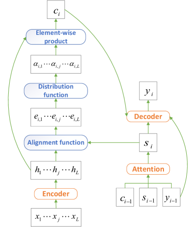
Figure 3: Attention mechanism structure

First, the input sequence $(x_{1},x_{2},\ldots,x_{L})$ is encoded by encoder and transformed to $(h_{1},h_{2},\ldots,h_{L})$. Then, the hidden states $\{s_{i}\}_{i=1}^{T}$ of decoder is generated by the attention network, and the corresponding weights $\{\alpha_{i,j}\}_{j=1}^{L}$ of encoder states in the $i$-th time step are calculated by $s_{i}$. The context vector $c_{i}$ consists of a linear combination of attention weights $\{\alpha_{i,j}\}_{j=1}^{L}$ and encoder states $\{h_{j}\}_{j=1}^{L}$. Finally, the decoder generates the output token $y_{i}$ using the current time step context vector $c_{i}$ and hidden state $s_{i}$.

Since the order and position of input text and output speech in TTS task are corresponding, attention alignment in TTS is a surjective mapping from the output frames to the input tokens and should follow such strict criteria He et al. (2019):

• Locality Each output frame should be aligned around a single input token to avoid attention collapse.

• Monotonicity The position of the aligned input token must never rewind backward to prevent repeating.

• Completeness Each input token should be covered once or aligned with some output frame to avoid skipping.

The original Tacotron model uses the content-based attention mechanism proposed by Bahdanau et al. (2014). In this case, Eq. (4) is:

$$e_{i,j}=v^{T}tanh(Ws_{i}+Vh_{j}+b)$$ (8)

where $Ws_{i}$ and $Vh_{j}$ represent query and key, respectively.

The content-based attention mechanism does not consider the position information of each item in the sequence at all, and can not effectively utilize the monotonicity and locality of alignment, thus alignment errors are common. In order to enable the attention mechanism to consider the positon information of input and output, and thus enhance the generalization ability of synthesizing long sentences, Char2wav Sotelo et al. (2017), Voiceloop Taigman et al. (2017) and Melnet Vasquez and Lewis (2019) adopted the Gaussian mixture model (GMM) attention mechanism proposed by Graves (2013) to replace the content-based attention mechanism in Tacotron. This method is a purely location-based attention mechanism, which uses an unnormalized mixture of $K$ Gaussians to produce the attention weights, $\alpha_{i,j}$, for each encoder state:

$$\alpha_{i,j}=\sum_{k=1}^{K}\frac{w_{i,k}}{Z_{i,k}}exp\Big{(}-\frac{(j-\mu_{i,k})^{2}}{2(\sigma_{i,k})^{2}}\Big{)}$$ (9)

$$\mu_{i,k}=\mu_{i-1,k}+\Delta_{i,k}$$ (10)

where $w_{i,k}$, $Z_{i,k}$, $\Delta_{i,k}$ and $\sigma_{i,k}$ are computed from the attention RNN state. The mean of each Gaussian component $\mu_{i,k}$ is computed using the recurrence relation in Eq. (10), which makes the mechanism location-relative and potentially monotonic if $\Delta_{i,k}$ is constrained to be positive. Although this location-based attention mechanism can enhance the generalization ability of acoustic models for long sentences, it sacrifices some of the naturalness of synthesized speech.

In order to combine content and location information in alignment, Tacotron 2 uses the hybrid location-sensitive attention mechanism Chorowski et al. (2015). In this case, Eq. (4) is:

$$e_{i,j}=v^{T}tanh(Ws_{i}+Vh_{j}+Uf_{i,j}+b)$$ (11)

where $Uf_{i,j}$ represents the location-sensitive term, and uses convolutional features computed from the previous attention weights $\{\alpha_{i-1,j}\}_{j=1}^{L}$. This method combines the content and location features to make alignment more accurate by additionally introducing previous attention weight information.

Based on the monotonicity of alignment between input and output sequences in TTS, various monotonic attention mechanisms have been proposed to reduce errors in attention alignment. In order to introduce monotonicity into the hybrid location-sensitive attention, Battenberg et al. (2020) proposed Dynamic Convolution Attention (DCA), which removed content-based terms $Ws_{i}$ and $Vh_{j}$, leaving only location-sensitive term $Uf_{i,j}$ as static filters, while adding a set of learned dynamic filters $Tg_{i,j}$ and a single fixed prior filter $p_{i,j}$. In this case, Eq. (4) is redefined as:

$$e_{i,j}=v^{T}tanh(Uf_{i,j}+Tg_{i,j}+b)+p_{i,j}$$ (12)

Similar to static filters $Uf_{i,j}$, dynamic filters $Tg_{i,j}$ are computed from the attention RNN state and serve to dynamically adjust the alignment relative to the alignment at the previous step. Prior filter $p_{i,j}$ is used to bias the alignment toward short forward steps. This monotonic DCA has stronger generalization ability and is more stable.

Raffel et al. (2017) proposed a monotonic alignment method that can be applied to TTS: monotonic attention (MA). At each step $i$, MA inspects the memory entries from the memory index $t_{i-1}$ it focused on at the previous step and evaluates the ”selection probability” $p_{i,j}$:

$$p_{i,j}=\sigma({e_{i,j}})$$ (13)

where $\sigma$ is logistic sigmoid function and energy values $e_{i,j}$ are produced as in Eq. (4). Starting from $j=t_{i-1}$, at each time MA would sample $z_{i,j}\sim Bernoulli(p_{i,j})$ to decide to keepj unmoved $(z_{i,j}=1)$ or move to the next position $(z_{i,j}=0)$. j would keep moving forward until reaching the end of inputs, or until receiving a positive sampling result $z_{i,j}=1$, and when j stops, memory $h_{j}$ would be directly picked as $c_{i}$. With such restriction, it is guaranteed that solely one input unit would be focused on at each step, and its position would never rewind backward. Moreover, the mechanism only requires linear time complexity and supports online inputs, which could be efficient in practice.

In contrast to the traditional “soft” attention using continuous weights, MA, which simply selects one input unit as the context vector $c_{i}$, is a “hard” attention. It can ensure the locality of attention alignment, but it could not be trained by standard back-propagation (BP) algorithm. Multiple approaches have been proposed for this issue, including reinforcement learning Xu et al. (2015); Zaremba and Sutskever (2015); Ling (2017), approximation by beam search Shankar et al. (2018), and approximation by soft attention for training Raffel et al. (2017).

To further guarantee the completeness of alignment, He et al. (2019) proposed stepwise monotonic attention (SMA), which adds additional restrictions on MA: in each decoding step, the attention alignment position moves forward at most one step, and it is not allowed to skip any input unit. The alignment of soft attention (SA), MA and SMA is shown in Fig. 4 He et al. (2019). The color depth of each node in the figure represents the size of the attention weight between each output acoustic feature frame and the input phoneme. The darker the color, the greater the value of attention weight. The figure shows that each acoustic feature frame is calculated by multiple input phonemes in SA. Each acoustic feature frame is determined by an input phoneme in MA. In SMA, not only each acoustic feature frame is determined by an input phoneme, but all input phonemes must be corresponding at least once, which ensures the locality, monotonicity and completeness of attention alignment.

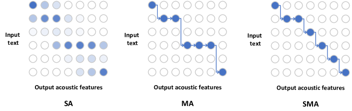
Figure 4: The alignment of SA, MA and SMA

Zhang et al. (2018b) and Yasuda et al. (2019) also proposed similar monotonic attention mechanisms. Zhang et al. (2018b) suggested that only the alignment paths satisfying the monotonic condition are taken into consideration at each decoder time step. The attention probabilities of each time step can be computed recursively using a forward algorithm, and a transition agent is proposed to help the attention mechanism make decisions whether to move forward or stay at each decoder time step. This attention mechanism has the advantages of fast convergence speed and high stability. Yasuda et al. (2019) also proposed a hard monotonic attention mechanism. The framework and likelihood function are similar to those of a hidden Markov model (HMM). The constrained alignment is conceptually borrowed from segment-to-segment neural transduction (SSNT) Yu et al. (2016b, a). They factorized the generation probability for acoustic features into an alignment transition probability and emission probability, thereby constraining the alignment process to moving from left to right, and only one step at a time. Although this hard monotonic alignment method can avoid some alignment errors that are commonly observed in soft-attention-based methods, including muffling, skipping, and repeating, this attention mechanism has poor stability and long training time.

In order to make more direct use of the correspondence between text and speech in TTS, Tachibana et al. (2018) and Wang (2019) added a guided attention loss to content-based dot product attention Vaswani et al. (2017). More specifically, they added an additional monotonic attention loss to the original audio reconstruction loss, forcing the non-zero values of the attention weight matrix were concentrated on the diagonal as much as possible. Furthermore, the forced increment attention was proposed to force the text and speech to be aligned monotonously by making the corresponding text position of acoustic feature frame at each time step move forward by at most one. To produce monotonic alignment, Deep Voice 3 and ParaNet added positional encoding in Transformer to the content-based dot product attention. Besides, they added an attention window Liu et al. (2019b); Merboldt et al. (2019) he attention during inference, calculated the attention weights only for the input characters in the window, and took the position of the character with the largest attention weight as the starting position of the next window. Moreover, ParaNet adopted a multi-layer attention mechanism to iteratively refine attention alignment in a layer-by-layer manner.

However, the use of positional encoding can cause errors when synthesizing long sentences Li et al. (2020). To synthesize long sentences stably, Glow-TTS removes the positional encoding and adds relative position representations Shaw et al. (2018) into self-attention modules instead. RobuTrans Li et al. (2020) counts on the 1-D CNN used in Encoder Pre-net to model relative position information in a fixed window. Moreover, in order to make the self-attention in Transformer more suitable for TTS models, RobuTrans also uses Pseudo Non-causal Attention (PNCA) to replace the traditional causal self-attention. The decoding process is more robust by providing the decoder with the holistic view of the input sequence and the frame-level context information.

As described in Sect. 3.1.2, a large number of non-autoregressive acoustic models have been proposed recently. TTS is a one-to-many mapping. For the same text input, there are many possible speech expressions with different prosody. To eliminate ambiguity in multi-mode output, the acoustic models with autoregressive decoders can predict the acoustic feature frames of the next time step by combining the contextual information provided by the acoustic feature frames generated by the previous time step. However, acoustic models with non-autoregressive decoders need to obtain contextual information in other ways to select an appropriate generation mode. Non-autoregressive acoustic models need to determine the output length in advance, rather than predict whether to stop at each frame. In this case, in order to align the inputs and outputs, a duration predictor similar to the one used in the traditional SPSS method Ze et al. (2013); Zen et al. (2009) can be used instead of the attention network. Aligning with a duration predictor can avoid the errors of skipping, repeating, and irregular stops caused by the attention mechanism. This method first appeared in NMT Gu et al. (2018), and then was introduced into TTS through non-autoregressive acoustic models such as FastSpeech Ren et al. (2019a). Acoustic models with duration predictors can align input phonemes and output acoustic features by introducing additional alignment modules or using external aligners. Next, these two alignment methods are introduced separately.

The most direct way to obtain the alignment information is provided by an external aligner. For example, FastSpeech extracts phoneme duration from a pre-trained autoregressive model by knowledge distillation Kim and Rush (2016). However, FastSpeech lacks generalization ability for long utterances, especially those whose length exceeds the maximum length of the utterance in the training set. This may be because the self-attention is a global modeling method. To use the local modeling method to make network more stable, DeviceTTS Huang et al. (2020) replaces the Transformer with DFSMN, which makes use of a latency control window size to learn the context. To simplify the training process, JDI-T Lim et al. (2020) jointly trains the autoregressive Transformer teacher network and the feed-forward Transformer student network. To avoid the complicated knowledge distillation process, some models use a separate external alignment model to predict the target phoneme duration, thus establishing alignment between input phonemes and output acoustic features. For example, TalkNet Beliaev et al. (2020) uses the CTC-based automatic speech recognition (ASR) model Quartznet Kriman et al. (2020), FastSpeech 2 Ren et al. (2020) uses the forced-alignment tool MFA toolkit McAuliffe et al. (2017), DurIAN Yu et al. (2019) uses a external alignment model Zen et al. (2016); Fan et al. (2014), RobuTrans Li et al. (2020) uses speech recognition tools, Parallel Tacotron Elias et al. (2020) and Non-Attentive Tacotron Shen et al. (2020) use a speaker-dependent HMM-based aligner with a lexicon Wightman and Talkin (1997). To address the difficulty of training an aligner due to data sparsity, Shen et al. (2020) used fine-grained VAE (FVAE) to achieve semi-supervised and unsupervised duration prediction, that is, simply train the model using the predicted durations instead of the target durations for upsampling.

It is also possible to directly learn alignment by training an alignment module within the model. For example, AlignTTS Zeng et al. (2020) uses the dynamic programming to consider all possible alignments in training, that is, uses the alignment loss inspired by the Baum-Welch algorithm Taylor (2009); Baum et al. (1970) to train the mix density network for alignment. Glow-TTS uses the Monotonic Alignment Search (MAS) algorithm to predict the duration of each input tokens by searching for the most probable monotonic alignment between text and the latent representation of speech. The internal alligator of EATS Donahue et al. (2020) implicitly enhances the monotonicity of alignment by predicting token lengths and obtaining positions using a cumulative sum operation. Moreover, the dynamic time warping (DTW) loss and the aligner length loss are introduced to learn alignment and ensure that the model can accurately predict phoneme lengths. Flow-TTS Miao et al. (2020) trains a length predictor inside the model to predict the output length in advance, and takes the positional encoding of the predicted spectrogram length as query vector to align the input and output using the positional attention module based on the multi-head dot-product attention mechanism Vaswani et al. (2017).

Since one-to-many regression problems like TTS can benefit from autoregressive decoding, it is also possible to combine the autoregressive method with duration predictor to further improve the stability of TTS models, such as the alignment methods used in DurIAN, Non-Attentive Tacotron Shen et al. (2020), DeviceTTS and RobuTrans Li et al. (2020). The alignment method of each model is shown in Table 2.

Table 2: Alignment method of each acoustic model

Acoustic model	Neural network types	Generative model types	Alignment methods	Characteristics
Tacotron (Wang et al., 2017)	CBHG, GRU	Autoregression	Content-based attention	Unstable, alignment errors often occur
Char2Wav (Sotelo et al., 2017)	RNN	Autoregression	GMM attention	Low naturalness of synthesized speech
Deep Voice 3 (Ping et al., 2017)	CNN	Autoregression	Dot-product attention, positional encoding, attention window	Attention is monotonic
VoiceLoop (Taigman et al., 2017)	Shifting buffer	Autoregression	GMM attention	Low naturalness of synthesized speech
DCTTS (Tachibana et al., 2018)	CNN	Autoregression	Dot-product attention and guided attention	Stable, alignment errors are rare
Tacotron 2 (Shen et al., 2018)	LSTM, CNN	Autoregression	Mixed location-sensitive attention	Able to synthesize long sentences accurately
DurIAN (Yu et al., 2019)	CBHG, RNN	Autoregression	Duration prediction model, external alignment model	Stable, alignment errors are rare
FastSpeech (Ren et al., 2019a)	Transformer	Non-autoregression	Duration prediction model, knowledge distillation	Errors will occur when synthesizing long sentences
FastSpeech 2 (Ren et al., 2020)	Transformer	Non-autoregression	Duration prediction model, MFA toolkit	Stable, alignment errors are rare
ParaNet (Peng et al., 2020)	CNN	Non-autoregression	Dot-product attention, positional encoding, attention window, multi-layer attention, knowledge distillation	Attention alignment is monotonic and stable
EATS (Donahue et al., 2020)	CNN	GAN	Duration prediction model, internal alignment module	Stable, alignment errors are rare
Non-Attentive Tacotron (Shen et al., 2020)	RNN	Autoregression	Duration prediction model, external alignment module	Stable, alignment errors are rare
FastPitch (Łańcucki, 2020)	Transformer	Non-autoregression	Duration prediction model, knowledge distillation	Can control the pitch contour of synthesized speech
Glow-TTS (Kim et al., 2020)	Transformer, Glow	Normalizing flow	Duration prediction model, MAS algorithm	The alignment is monotonic and stable
AlignTTS (Zeng et al., 2020)	Transformer	Non-autoregression	Duration prediction model, internal alignment module	Stable, alignment errors are rare
SpeedySpeech (Vainer and Dušek, 2020)	CNN	Non-autoregression	Duration prediction model, knowledge distillation	Stable, alignment errors are rare
JDI-T (Lim et al., 2020)	Transformer	Non-autoregression	Duration prediction model, knowledge distillation	Joint training of teacher and student network, stable and alignment errors are rare
TalkNet (Beliaev et al., 2020)	CNN	Non-autoregression	Duration prediction model, ASR model	Stable, alignment errors are rare
Flow-TTS (Miao et al., 2020)	Glow	Normalizing flow	Multi-head dot-product attention, internal length predictor	High quality of synthesized speech, fast training and inference speed
DeviceTTS (Huang et al., 2020)	DFSMN, RNN	Combination of autoregression and non-autoregression	Duration prediction model	Stable, alignment errors are rare
Parallel Tacotron (Elias et al., 2020)	LConv	Non-autoregression	Duration prediction model, HMM-based aligner	Stable, alignment errors are rare
RobuTrans (Li et al., 2020)	Transformer	Autoregression	Duration prediction model, speech recognition tools	Stable, alignment errors are rare

3.3 Expressive acoustic model

The speech synthesized by deep learning method has a smooth tone, without rhythm and expressiveness, thus it often has a certain gap with the real human voice. In order to synthesize expressive speech, three parts need to be considered: ”what to say”, ”who to say” and ”how to say”. ”What to say” is controlled by the input text and the text front-end. ”Who to say” can be controlled by collecting a large amount of voice data of a person and then training the model to learn to imitate the speaker’s voice. ”How to say” is controlled by prosodic information such as tone, speech rate, and emotion of the synthesized speech. In this paper, ”who to say” and ”how to say” are collectively referred to as the style features of synthesized speech.

3.3.1 Acoustic model with reference encoder

Style information can be introduced by adding a reference encoder to synthesize expressive speech. There are mainly two methods based on reference encoders that can be used to synthesize speech with a specific style. The first method is to directly control various speech style parameters, such as pitch, loudness, and emotion, by using a trained reference encoder. The second method is to input the reference audio into the reference encoder and use the style parameters encoded by the reference encoder to transfer the speech style features between the reference speech and the target speech. Different methods and models have been proposed to disentangle the different style feature information so that each style feature can be easily controlled individually to synthesize speech with the target style. These methods and models are described in the following paragraphs.

Skerry-Ryan et al. (2018) divided the features of speech into three components: text, speaker, and prosody. A reference encoder is added to tacotron to extract the prosody embedding from the reference speech with a specific style, and the speaker embedding is obtained by using a speaker embedding lookup table. Then the prosody embedding, speaker embedding and text embedding are combined and input into the decoder to synthesize speech with the style of the reference speech. Gururani et al. (2019) refined the model on the basis of Skerry-Ryan et al. (2018), divided the style features of speech into pitch and loudness, and selected two 1-D time series to model the fundamental frequency $f_{0}$ and loudness of the reference speech respectively. In order to transfer the emotion features in the reference speech more accurately, Li et al. (2021) added two emotion classifiers after the reference encoder and decoder respectively to enhance emotion classification ability in the emotion space. Moreover, they adopted a style loss Johnson et al. (2016); Gatys et al. (2015) to measure the style differences between the generated and reference mel-spectrogram Ma et al. (2018b); Gatys et al. (2016).

Voice conversion (VC) model can disentangle the speaker-dependent timbre feature from speech Chou et al. (2018, 2019); Qian et al. (2019); Serrà et al. (2019); Kameoka et al. (2018), but cannot extract other style features such as the content, pitch and rhythm of speech. Inspired by the voice conversion model AutoVC Qian et al. (2019), Qian et al. (2020) proposed SPEECHFLOW, which is a speech style conversion model that can disentangle the rhythm, pitch, content, and timbre information. Rhythm, pitch and content features are extracted by three encoders respectively, and timbre feature is represented by one-hot vector of speaker ID. SPEECHFLOW can be trained for speech style conversion by replacing the input of the three encoders with the spectrogram or pitch contour of the reference speech.

Similarly, in order to disentangle different style features in speech and achieve the purpose of individually controlling each feature, Wang et al. (2018b) introduced a global style token (GST) network in Tacotron, which plays a role of clustering. When the GST network is trained with speech data with various styles, multiple meaningful and interpretable tokens can be obtained. The weighted sum of these tokens is used as a style embedding to control and transfer the style features of speech. In inference, a specific weight can be chosen directly for each style token, or a reference signal can be fed to guide the choice of token combination weights. For the choice of token weight, Kwon et al. (2019a) proposed a controlled weight (CW)-based method to define the weight values by investigating the distribution of each emotion in the emotional vector space. Um et al. (2020) proposed to improve the method of simply averaging the style embedding vectors belonging to each emotion category Kwon et al. (2019b) to determine the representative weight vectors by maximizing the ratio of inter-category distance to intra-category distance (I2I), and proposed to apply the spread-aware I2I (SA-I2I) method to change the emotion intensity instead of the simple linear interpolation-based approach. Mellotron Valle et al. (2020a) additionally introduces fundamental frequency $f_{0}$ information, and takes text, speaker, fundamental frequency $f_{0}$, attention mapping, and GST as conditions when synthesizing speech, in which the speaker represents timbre, the fundamental frequency $f_{0}$ represents pitch, the attention mapping represents rhythm, and GST represents prosody.

Since GST-Tacotron uses only paired input text and reference speech for training, inputting unpaired text and speech during synthesis will cause the generated sound to become blurry. Moreover, in this case, the reference encoder may store some text information in the reference embedding rather than prosody and speaker information to reconstruct the input speech. Using the idea of dual learning, Liu et al. (2018) proposed to train GST-Tacotron with unpaired text and speech, and input the output mel-spectrogram into the ASR model to predict the input text, thus preventing the reference encoder from encoding any text information. Furthermore, they also use the regularization method of attention consistency loss to accelerate the training convergence speed of both ASR and TTS models.

In order to control the style of synthesized speech more flexibly, multiple reference encoders can be used to extract different style features of multiple reference speech respectively. For example, Bian et al. (2019) used multiple reference encoders based on GST network to disentangle different style features, and proposed intercross training technique to separate the style latent space by introducing orthogonality constraints between the extracted styles of each encoder. However, this intercross training scheme does not guarantee each combination of style classes is seen during training, causing a missed opportunity to learn disentangled representations of styles and sub-optimal results on disjoint datasets. Whitehill et al. (2019) used an adversarial cycle consistency training scheme to ensure the use of information from all style dimensions to address the challenges of multi-reference style transfer on disjoint datasets. They achieved a higher rate of style transfer for disjoint datasets than previous models.

Variational auto-encoder (VAE) Kingma and Welling (2013) generates samples with specific features by sampling from the distribution of latent variables. Latent variables are continuous and can be interpolated, similar to the implicit style features in speech. The speech style features learned by VAE in an unsupervised manner can be easily separated, scaled and combined. Therefore, there are many tasks that use VAE to control the synthesized speech style. The speech style features learned by VAE in an unsupervised manner can be easily separated, scaled and combined. Therefore, there are many works using VAE to control the style of synthesized speech. For example, Zhang et al. (2019c) added a VAE network to Tacotron 2 to learn latent variables representing speech style. Each dimension of latent variables represents a different style feature. In order to further disentangle the various style features of speech, Hsu et al. (2019) proposed GMVAE-Tacotron based on the Gaussian mixture VAE network, with two levels of hierarchical latent variables. The first level is a discrete latent variable, representing a certain category of style (e.g. speaker ID, clean/noisy). The second level is a continuous latent variable approximated by the multivariate Gaussian distribution. Each component represents the degree of the feature (e.g. noise level, speaking rate, pitch) under the category of the first level. In general, it is equivalent to using the GMM to fit the distribution of latent variables. This model can effectively factorize and independently control latent attributes underlying the speech signal.

However, these methods only model the global style features of speech, without considering prosodic control at the phoneme and word levels. In order to model acoustic features at various resolutions, Sun et al. (2020), in addition to modeling global speech features such as noise and channel number, also modeled word-level and phoneme-level prosodic features such as fundamental frequency $f_{0}$, energy and duration. They used a conditional VAE with an autoregressive structure to make prosodic features of each layer more interpretable and to impose hierarchical conditioning across all latent dimensions. Parallel Tacotron Elias et al. (2020) used two different VAE models, one similar to Hsu et al. (2019) for modeling global features of speech such as different prosodic patterns of different speakers, and the other similar to Sun et al. (2020) for modeling phoneme-level fine-grained features.

Normalizing flow can control the latent variables to synthesize speech with different styles by learning an invertible mapping of data to a latent space. For example, Flowtron Valle et al. (2020b) applied the normalizing flow to Tacotron to control speech variation and style transfer by learning a latent space that stores non-textual information. Glow-TTS Kim et al. (2020) takes Glow Kingma and Dhariwal (2018) as the decoder to control the style of synthesized speech by controlling the prior distribution of latent variables. It is also possible to model speech style features with both normalizing flow and VAE. Aggarwal et al. (2020) used VAE and Householder Flow Tomczak and Welling (2016) to improve the reference encoder proposed by Skerry-Ryan et al. (2018), thereby enhancing the disentanglement capability of the TTS system.

GAN can also be used in style speech synthesis. For example, Ma et al. (2018b) enhanced the content-style disentanglement ability and controllability of the model by combining a pairwise training procedure, an adversarial game, and a collaborative game into one training scheme. The adversarial game concentrates the true data distribution, and the collaborative game minimizes the distance between real samples and generated samples in both the original space and the latent space.

3.3.2 Acoustic model of explicit modeling style features

The prosody of the speech can also be controlled intuitively by constraining the prosodic features of the waveform. For example, Morrison et al. (2020) proposed a user-controllable, context-aware neural prosody generator that allows the input of the $f_{0}$ contour for certain time frames and generates the remaining time frames from input text and contextual prosody. CHiVE Kenter et al. (2019) is a conditional VAE model with a hierarchical structure. It can generate prosodic features such as fundamental frequency $f_{0}$, energy $c_{0}$ and duration suitable for use with a vocoder, and yield a prosodic space from which meaningful prosodic features can be sampled. To efficiently capture the hierarchical nature of the linguistic input (words, syllables and phones), both the encoder and decoder parts of the auto-encoder are hierarchical, in line with the linguistic structure, with layers being clocked dynamically at the respective rates.

In practical applications, since it is difficult to interpret and give practical meaning to each of the latent variables learned by unsupervised style separation methods such as GST and VAE, FastSpeech uses a length adjuster to replicate and expand the hidden state of the phoneme sequence according to the duration of each phoneme, thus intuitively controlling the speech speed and some prosodic features.

FastPitch Łańcucki (2020) adds a pitch prediction network to FastSpeech to control pitch. Compared with FastSpeech and FastPitch, FastSpeech 2 introduces more style features such as pitch, energy, and more accurate duration as conditional inputs to construct a variance adaptor, and uses trained predictors of energy, pitch, and duration predictors to synthesize speech with a specific style. Durian simply divides speech styles into several discrete categories, learns embedding vectors from speech data with various styles through supervised learning , and controls the intensity of the style by multiplying a scalar.

3.3.3 Multi-speaker acoustic model

Multi-speaker speech synthesis is also an important task of TTS model. A simple way to synthesize the voices of multiple speakers is to add a speaker embedding vector to the input Gibiansky et al. (2017); Ping et al. (2017). The speaker embedding vector can be obtained by additionally training a reference encoder. For example, Jia et al. (2018), Arik et al. (2018) and Nachmani et al. (2018) introduced a speaker encoder in Tacotron 2, Deep Voice 3 and VoiceLoop Taigman et al. (2017) respectively to encode the speaker information in the reference speech into a fixed-dimensional speaker embedding vector. The embedding vector can be extracted only from a small number of speech fragments of the target speaker. The speech data corpus used to train the speaker encoder only needs to contain the recordings of a large number of speakers, but does not need to be of high quality. Even if the training data contains a small amount of noise, the extraction of timbre features will not be affected.

The speaker adaptation can also be used for multi-speaker speech synthesis. Arik et al. (2018), Taigman et al. (2017), and Zhang et al. (2020c) fine-tune the trained multi-speaker model using a small number of $\langle$text, speech$\rangle$ data pairs of the target speaker. Fine-tuning can be applied to the speaker embedded vector Arik et al. (2018); Taigman et al. (2017), part of the model Zhang et al. (2020c), or the whole model Arik et al. (2018). Moss et al. (2020) proposed a fine-tuning method to select different model hyperparameters for different speakers, achieving the goal of synthesizing the voice of a specific speaker with only a small number of speech samples, in which the selection of hyperparameters adopts the Bayesian optimization method Shahriari et al. (2015).

However, these methods are not very effective when synthesizing the speech of unseen speakers. To solve this problem, Cooper et al. (2020) extracted speaker information by using learnable dictionary encoding (LDE) on the basis of Jia et al. (2018), and inserted the speaker embedding into both prenet layer and attention network of Tacotron 2 as additional information. When training the speaker encoder, Nachmani et al. (2018) introduced, in addition to the use of MSE losses, the contrast loss term and the cyclic loss term, which allowed the model to synthesize the voice of the new speaker with only a small amount of audio. When training the speaker encoder, in addition to the MSE loss, Nachmani et al. (2018) also a contrastive loss term and a cyclic loss term, which allow the model to synthesize the voice of a new speaker with only a small amount of audio. Cai et al. (2020) and Shi et al. (2020) introduced an identity feedback constraint by adding an additional loss term between the reference embedding and the extraction embedding of the synthesized signal, thus increasing the robustness and speaker similarity of the produced speeches.

3.4 Low-resource acoustic model

Deep learning based acoustic models need to be trained with a large number of high-quality $\langle$text, speech$\rangle$ data pairs to synthesize high-fidelity speech, and the data set requirements are higher when synthesizing speech with specific prosody and emotion. But for $95\%$ of languages and audio with a specific style, the corpus is very scarce. Moreover, the English speech corpus used for TTS usually contains about $10-40$ hours of speech data and contains no more than $20,000$ words. The largest public English speech corpus, LibriTTS Zen et al. (2019), contains only $80,000$ words, which is far lower than the number of words in the regular English vocabulary (usually $130,000-160,000$). When synthesizing, the acoustic model may mispronounce words outside the training set. It is difficult to cover all vocabulary just by increasing the number of training utterances, because the natural frequency of words tends to follow the Zipfian distribution Taylor and Richmond (2019), which means that the number of new words contained in the speech data per hour gradually decreases. Therefore, to achieve a linear increase in word coverage would require an exponential increase in audio data, which would be costly and impractical. Besides, most speech data is recorded by non-professionals and contains a lot of noise. Therefore, the lack of high-quality speech training data in TTS is mainly manifested in the lack of training data that cannot cover all vocabulary and contains noise.

To solve the problem that the speech data cannot cover all the words, text and phonemes can be input into the acoustic network together. During training, some words can be represented by text randomly, so that the acoustic model can predict the phoneme pronunciation of unseen words according to the learned correspondence between characters and phonemes Ping et al. (2017); Peng et al. (2020). The text front-end can also be used to convert the text into phonemes in advance, in order to make the model only need to learn the pronunciation of a small number of phonemes.

To solve the problem of the lack of speech data for minority languages and dialects, the method of cross-language transfer learning can be used. For example, Guo et al. (2018) and Zhang et al. (2019b) trained an average language model with a large Mandarin corpus and a small Tibetan corpus when training the Tibetan TTS model, which made up for the lack of Tibetan speech data. Tu et al. (2019) introduced cross-language transfer learning into Tacotron. They used speech data from high-resource languages to pre-train Tacotron, and then fine-tuned the pre-trained model with speech data from low-resource languages. Nekvinda and Dušek (2020) used the idea of meta-learning to train the acoustic model with only a small number of samples from multiple languages in order to synthesize speech containing multiple languages. They used a fully convolutional encoder from DCTTS, whose parameters are generated using a separate contextual parameter generator network Platanios et al. (2018) conditioned on language embedding, thus realizing cross-lingual knowledge-sharing.

Semi-supervised pre-training can also be used to reduce the demand of the TTS model for paired training data. Chung et al. (2019) proposed training the encoder and decoder with unpaired text and speech respectively, and then fine-tuning the pre-trained Tacotron with a small amount of $\langle$text, speech$\rangle$ data pairs. Although this approach helps the model synthesizes more intelligible speech, the experimental results show that pre-training the encoder and decoder separately at the same time does not bring further improvement than only pre-training the decoder. And there is a mismatch between pre-training only the decoder and fine-tuning the whole model, because during pre-training the decoder is only conditioned on the previous frame, while during fine-tuning the decoder is also conditioned on the text representation output by the encoder. To avoid potential error caused by this mismatch and further improve the data efficiency by using only speech, Zhang and Lin (2020) proposed to use vector Vector-quantization Variational-Autoencoder (VQ-VAE) Chorowski et al. (2019); Oord et al. (2017) to extract unsupervised linguistic units from untranscribed speech and then use $\langle$linguistic units, speech$\rangle$ pairs to pre-train the entire model. The language units act as phonemes that are paired with the audio, while VQ-VAE plays a role similar to speech recognition model. However, VQ-VAE is trained in an unsupervised way to obtain discretized linguistic representations, which is suitable for low-resource languages. Finally, the model is fine-tuned with a small amount of $\langle$text, speech$\rangle$ data pairs.

Using dual learning to train TTS and ASR models simultaneously can also achieve the purpose of using text or speech data alone to train both models. Tjandra et al. (2017) proposed an auto-encoder model in which one is regarded as an encoder and the other as a decoder. For example, when there is only speech but no corresponding text, the ASR model can be used as the encoder to output text, and the TTS model can be used as the decoder to output speech, and then the speech output of the TTS model is expected to be as close as possible to the input speech. The other situation is similar when there is only text but no speech. Ren et al. (2019b) also used the idea of dual learning to combine TTS and ASR to build the capability of the language understanding and modeling in both speech and text domains using unpaired data during training, that is, using denoising auto-encoder (DAE) to reconstruct corrupt speech and text in an encoder-decoder framework. They also used a dual transformation (DT) approach similar to Tjandra et al. to train the model to convert text to speech and speech to text respectively. The difference is that Tjandra et al. relied on two well-trained TTS and ASR models, whereas Ren et al. trained the two models from scratch, which is suitable for the lack of training data.

Multi-speaker TTS model has much lower requirements on the quantity and quality of training data than models that synthesize speech with a specific style, because they only need to separate and capture timbre information in the audio. However, if the speech training data of the target speaker is too small, the timbre features cannot be effectively learned. In order to increase the amount of speech data of the target speaker, Huybrechts et al. (2020) used a voice conversion (VC) model to convert the voice data of other speakers into the voice of the target speaker for data augmentation, then trained the TTS model with the expanded speech data, and finally used the real voice data of the target speaker for fine-tuning.

The noise in the training data can be reduced by pre-processing steps. Valentini-Botinhao and Yamagishi (2018) took the acoustic features of clean speech and noisy speech respectively as the input and target of RNN network, enabling the network to convert noisy speech into clean speech. Generally, the data in the corpus containing different styles of speech is of low quality and contains noise, which will hinder the training of style speech synthesis model. In this case, the method of speech style control introduced in Sect. 3.3.1 can be used to train the style extraction network with clean data and noisy data. By making the network learn about the latent variables of noise features, it can synthesize clean speech. For example, Wang et al. (2018b) trained GST-Tacotron by using data sets mixed with various noises to learn tokens about the noise features. During synthesis, the token representing noiseless is used as the style embedding to convert noisy reference speech to clean speech. Hsu et al. (2019) used one dimension of the mixed Gaussian distribution to represent the noise feature. Clean speech can be synthesized by using the average value of the clean speech class or the value of the noise variable extracted from the clean reference speech as the value of the noise feature.

4 Vocoder

Inspired by the successful application of autoregressive generative model Van Oord et al. (2016) in the field of image and natural language generation, Oord et al. (2016) first applied this method to TTS and proposed the most widely used vocoder WaveNet. In order to capture the long-range temporal dependencies in audio signals, WaveNet adopts a multi-layer dilated causal gated convolutional network, which makes the receptive field to grow exponentially with the depth. WaveNet uses speaker identity and linguistic features as global and local conditions respectively to synthesize the speech of the target speaker and text. However, WaveNet has a complex network structure and is autoregressive, therefore the training and inference speed is slow. Moreover, the speech synthesized with WaveNet is sometimes not natural. Therefore, after it was proposed, there are a lot of work to improve it. The direction of improvement is mainly to accelerate the speed of training and inference and improve the quality of synthesized speech, which are respectively called fast vocoder and high-quality vocoder. These methods are introduced in the following sections.

4.1 Fast vocoder

The training can be accelerated by reducing the size and parameters of the vocoder, and the inference can be accelerated by replacing the autoregressive method in WaveNet with non-autoregressive methods. The following sections will introduce various small-size vocoders and non-autoregressive vocoders.

4.1.1 Small size vocoder

To improve the speed of training and inference, Fftnet Jin et al. (2018) uses the simple ReLU activation function and $1\times 1$ convolutions to replace the gated activation units and dilated convolutions in WaveNet, which reduces the computational cost. SampleRNN Mehri et al. (2016) adopted a multi-scale RNN structure. Different layers operate on audio data of different time scales. Compared with WaveNet, it only processes individual samples in the last layer to improve the synthesis speed, and back-propagates the gradient of the loss function only on a small fraction of audio to improve the training speed. WaveRNN Kalchbrenner et al. (2018) only uses a single-layer GRU network with a dual softmax layer that predict respectively the 8 coarse (or more significant) bits and the 8 fine (or least significant) bits of the 16-bit audio sample, and applies a weight pruning technique to further reduce the model parameters. Furthermore, for the purpose of generating multiple channels of speech in parallel, WaveRNN divides a long audio sequence into multiple short sequences evenly during inference, and the generation within and between each short sequence is autoregressive. Although WaveRNN is autoregressive and based on RNN, its training and inference time is still short, thus it can be used in systems with few resources such as mobile phones and embedded systems. The Multi-Band WaveRNN proposed by Yu et al. (2019) further improves the inference speed of WaveRNN by generating multiple bands in parallel, and performs 8-bit quantization on the weight value to reduce the model size. LPCNet Valin and Skoglund (2019) reduces the complexity of the model by combining WaveRNN with linear prediction (LP) technology in traditional digital signal processing, thereby improving the synthesis efficiency. The characteristics of various small-size vocoders are shown in Table 3.

Table 3: Small size vocoder

Vocoder	Neural network types	Characteristics
WaveNet (Oord et al., 2016)	Dilated causal gated CNN	Based on dilated CNN, the training and inference speed is slow
SampleRNN (Mehri et al., 2016)	RNN	Multi-scale RNN structure, training and inference speed is faster than Wavenet
FftNet (Jin et al., 2018)	$1\times 1$ CNN	Based on $1\times 1$ convolution, the model structure is simple, and the training and inference speed is fast
WaveRNN (Kalchbrenner et al., 2018)	GRU	Based on single layer of GRU, the model structure is simple, and the training and inference speed is fast
Multi-Band WaveRNN (Yu et al., 2019)	GRU	Parallel generation of multiple bands, the training and inference speed is fast
LPCNet (Valin and Skoglund, 2019)	GRU	The linear prediction (LP) technology is used, the model structure is simple, and the training and inference speed is fast

4.1.2 Non-autoregressive vocoder

Similar to acoustic models, these vocoders increase the speed of training and inference to a certain extent, but all generate audio signals frame by frame in an autoregressive manner. If the non-autoregressive generation method can be used to generate speech waveforms in parallel, the inference speed will be greatly improved. Based on this idea, various non-autoregressive vocoders are proposed, and their characteristics are shown in Table 4.

Table 4: Non-autoregressive vocoder

Vocoder	Neural network types	Generative model types	Characteristics
WaveNet (Oord et al., 2016)	Dilated causal gated convolution	Autoregression	Autoregressive generation, slow training and inference speed
Parallel WaveNet (Oord et al., 2018)	Dilated causal gated convolution	IAF	Based on knowledge distillation, training and inference speed is fast, Monte Carlo sampling is required to estimate KL divergence, the training process is unstable
FloWaveNet (Kim et al., 2018)	Dilated convolution	Normalizing flow	The inference speed is fast, the training convergence speed is slow, the model contains many parameters
ClariNet (Ping et al., 2018)	Dilated causal gated convolution	IAF	Based on knowledge distillation, the training and inference speed is fast, the training process is stable
WaveGlow (Prenger et al., 2019)	Non-causal dilated convolution, $1\times 1$ convolution	Normalizing flow	The inference speed is fast, the training convergence speed is slow, the model contains many parameters
MelGAN (Kumar et al., 2019)	Dilated convolution, transposed convolution, grouped convolution	GAN	The inference speed is fast, the training convergence speed is slow
GAN-TTS (Bińkowski et al., 2019)	Dilated convolution	GAN	The training and inference speed is fast, no need for mel-spectrogram as input
Parallel WaveGAN (Yamamoto et al., 2020)	Non-causal dilated convolution	GAN	The inference speed is fast, the training convergence speed is slow, the model contains many parameters
WaveVAE (Peng et al., 2020)	Dilated causal gated convolution	IAF, VAE	The training and inference speed is fast
WaveFlow (Ping et al., 2020)	2D-dilated convolution	Autoregression	Combining the advantages of autoregressive flow and non-autoregressive flow, the training and inference speed is fast
WaveGrad (Chen et al., 2020)	Dilated convolution	Diffusion probability model	The inference speed is fast, the training convergence speed is slow
DiffWave (Kong et al., 2020b)	Bidirectional dilated convolution	Diffusion probability model	The inference speed is fast, the training convergence speed is slow
Multi-Band MelGAN (Yang et al., 2021)	Dilated convolution, transposed convolution, grouped convolution	GAN	The training and inference speed is fast

The traditional Gaussian autoregressive model is equivalent to an autoregressive flow (AF) Kingma et al. (2016), which is a kind of normalizing flow Rezende and Mohamed (2015). The main idea of the normalizing flow is that a complex distribution can be obtained by a simple distribution transformed through multiple invertible functions. It was originally proposed to make the distribution function of latent variables in VAE Kingma and Welling (2013) more complex. The flow-based generative model learns the bidirectional mapping from the input sample $x$ to the latent representation $\boldsymbol{z}$, i.e. $\boldsymbol{x}=f(\boldsymbol{z})$ and $\boldsymbol{z}=\boldsymbol{f}^{-1}(\boldsymbol{x})$. This mapping $\boldsymbol{f}$ is called a normalizing flow and is an invertible function fitted by neural networks, consisting of $k$ invertible transformations $\boldsymbol{f}=f_{1}\circ\cdots\circ f_{k}$. The normalizing flow transforms a simple density distribution $p(\boldsymbol{z})$ (such as an isotropic Gaussian distribution) to a complex distribution $p(\boldsymbol{x})$ by applying an invertible transformation $\boldsymbol{x}=\boldsymbol{f}(\boldsymbol{z})$. The probability density of $\boldsymbol{x}$ can be calculated through the change of variables formula:

$$p(\boldsymbol{x})=p(\boldsymbol{z})\Big{|}det\Big{(}\frac{\partial\boldsymbol{f}^{-1}(\boldsymbol{x})}{\partial\boldsymbol{x}}\Big{)}\Big{|}$$ (14)

where $det$ is the Jacobian determinant. The computation of the determinant has the complexity of $O(n^{3})$, where $n$ is the dimension of $\boldsymbol{x}$ and $\boldsymbol{z}$. In order to reduce the amount of computation, two flow models that can easily calculate the Jacobian determinant have been proposed, respectively, based on autoregressive transformation Van Oord et al. (2016) and bipartite transformation Kingma and Dhariwal (2018); Dinh et al. (2014, 2016).

During training, the autoregressive flow calculates the latent variable $z_{i},i=1,\ldots,D$ by transforming the speech $\boldsymbol{x}={x_{1},x_{2},\ldots,x_{D}}$:

$$z_{i}=\sigma_{i}(x_{1:i-1})\cdot x_{i}+\mu_{i}(x_{1:i-1})$$ (15)

where $z_{1:D}$ is $D$ latent variables subject to the isotropic Gaussian distribution, $\mu$ is the shift variables representing the mean, and $\sigma$ is the scaling variables representing the standard deviation. The training process is non-autoregressive, and $z_{i}$ only depends on $x_{1:i}$. In this case, the Jacobian matrix is a triangular matrix whose determinant is the product of the diagonal terms:

$$det\Big{(}\frac{\partial f^{-1}(\boldsymbol{x})}{\partial\boldsymbol{x}}\Big{)}=\prod_{i}\sigma_{i}(x_{1:i-1})$$ (16)

During inference, the trained $z_{i},i=1,\ldots,D$ and the previously generated audio $x_{1:i-1}$ are used to predict the new $x_{i}$:

$$x_{i}=\frac{z_{i}-\mu_{i}(x_{1:i-1})}{\sigma_{i}(x_{1:i-1})}$$ (17)

This inference process is autoregressive, resulting in slow inference. In order to speed up the inference speed, Parallel WaveNet Oord et al. (2018) and its improved model ClariNet Ping et al. (2018) use inverse autoregressive flow (IAF) Kingma et al. (2016) to generate speech in Parallel. IAF is another normalizing flow. In contrast to AF, IAF uses the previously obtained latent variable $z_{1:i-1}$ to calculate $z_{i}$ during training:

$$z_{i}=\frac{x_{i}-\mu_{i}(z_{1:i-1})}{\sigma_{i}(z_{1:i-1})}$$ (18)

This training process is autoregressive. In inference, $z_{1:i}$ is used to predict $x_{i}$:

$$x_{i}=\sigma_{i}(z_{1:i-1})\cdot z_{i}+\mu_{i}(z_{1:i-1})$$ (19)

This inference process is non-autoregressive. Therefore, AF is fast in training and slow in inference, whereas IAF is just the opposite. In order to train and synthesize quickly at the same time, Parallel WaveNet and ClariNet take the autoregression WaveNet as the teacher network, which is responsible for providing the guidance information on the distribution of $z_{i},i=1,\ldots,D$ during training. And IAF is used as the student network to take charge of the final audio sampling, and solve the problem that IAF cannot be trained in parallel by means of probability density distillation.

However, due to the knowledge distillation used in Parallel WaveNet and Clarinet, the training process is complex. In order to simplify the training process, Peng et al. (2020) proposed WaveVAE. The encoder and decoder of WaveVAE are respectively parameterized by a Gaussian autoregressive WaveNet and the one-step-ahead predictions from an IAF. It can jointly optimize the encoder $q_{\varphi}(\boldsymbol{z}|\boldsymbol{x})$ and decoder $p_{\theta}(\boldsymbol{x}|\boldsymbol{z})$ to be trained from scratch by maximizing the evidence lower bound (ELBO) for observed $\boldsymbol{x}$ in VAE, but at the expense of sound quality.

In order to train and synthesize more quickly, Ping et al. (2020) proposed WaveFlow which combines autoregressive flow and non-autoregressive convolution. The training process does not need complex knowledge distillation, only based on the likelihood function, and combines the advantages of autoregressive and non-autoregressive flow. It can train and synthesizing high- fidelity speech quickly, while only occupying small memory. WaveFlow represents a 1-D audio sequence $\boldsymbol{x}={x_{1},x_{2},\ldots,x_{D}}$ with a 2-D matrix $\boldsymbol{X}\in\boldsymbol{R}^{h\times w}$, in which adjacent samples are in the same column. The latent variable matrix $\boldsymbol{Z}\in\boldsymbol{R}^{h\times w}$ is defined as:

$$Z_{i,j}=\sigma_{i,j}(X_{1:i-1,:})\cdot X_{i,j}+\mu_{i,j}(X_{1:i-1,:})$$ (20)

where $X_{1:i-1,:}$ represents all the elements above the $i$-th row. Therefore, the value of $Z_{i,j}$ depends only on the sample in $i$-th row and $j$-th column and the samples above $i$-th row, which can be calculated at the same time. In inference, the sample is generated by:

$$X_{i,j}=\frac{Z_{i,j}-\mu_{i,j}(X_{1:i-1,:})}{\sigma_{i,j}(X_{1:i-1,:})}$$ (21)

Although it is autoregressive, it only takes $h$ steps to generate all samples, and $h$ is usually small, like 8 or 16. WaveFlow uses a 2-D dilated CNN to model a 2-D matrix. Non-causal CNN is used on width dimension, causal CNN with autoregressive constraints is used on height dimension, and convolution queue Paine et al. (2016) is used to cache the intermediate hidden states to speed up the autoregressive synthesis on height dimension. Therefore, it not only retains both the advantage of autoregressive inference method that can accurately simulate the local variations of waveform and non-autoregressive convolutional structure that can do speedy synthesis and capture the long-range structure in the data.

WaveGlow Prenger et al. (2019) and FloWaveNet Kim et al. (2018) are also based on normalizing flow and have similar structures, using Glow Kingma and Dhariwal (2018) and Real-NVP Dinh et al. (2016) respectively. Real-NVP is an improved model of the normalizing flow NICE Dinh et al. (2014). It is trained and inferred by bipartite transformation, but each layer can only transform a part of the input. As an improved model of Real-NVP, Glow introduces $1\times 1$ invertible CNN to mix the information between two channels and realizes complete transformation. The affine coupling layer in WaveGlow and Flowavenet transforms one half dimension $x_{b}$ of input vector $\boldsymbol{x}$ each time, leaving the other half dimension $x_{a}$ unchanged. The transformation process is:

$$z_{a}=x_{a}$$ (22)

$$z_{b}=x_{b}\cdot\sigma_{b}(x_{a})+\mu_{b}(x_{a})$$ (23)

where $x_{a}$ and $x_{b}$ are the result of bisecting $\boldsymbol{x}$, $z_{a}$ and $z_{b}$ are the corresponding latent variables respectively. The inference process is:

$$x_{a}=z_{a}$$ (24)

$$x_{b}=\frac{z_{b}-\mu_{b}(x_{a})}{\sigma_{b}(x_{a})}$$ (25)

Therefore, WaveGlow and FloWaveNet can both compute the latent variable $\boldsymbol{z}$ and synthesize the speech frame $\boldsymbol{x}$ in parallel. In fact, the bipartite transformation is a special autoregressive transformation Ping et al. (2020), which can be reduced to a bipartite transformation by substitution:

$$\left(\begin{array}[]{l}\mu_{i}(x_{1:i-1})\\ \sigma_{i}(x_{1:i-1})\end{array}\right)=\left\{\begin{array}[]{ll}(0,1)^{T},&i\in a\\ (\mu_{i}(x_{a}),\sigma_{i}(x_{a}))^{T},&i\in b\end{array}\right.$$ (26)

Compared with autoregressive transformation, bipartite transformation is not as expressive as autoregressive transformation, because it reduces the dependence between data $\boldsymbol{X}$ and latent variable $\boldsymbol{Z}$. As a result, the speech synthesized by WaveGlow and FloWaveNet is of low quality. A deeper network is needed to obtain the results comparable to the autoregressive model.

In addition to normalizing flow, GAN Goodfellow et al. (2014) can also be used to synthesize speech in parallel, such as Parallel WaveGAN Yamamoto et al. (2020), MelGAN Kumar et al. (2019), multi-band MelGAN Yang et al. (2021) and GAN-TTS Bińkowski et al. (2019). Parallel WaveGAN’s generator is similar in structure to WaveNet, which uses random noise and mel-spectrogram conditions to generate speech waveforms. Its discriminator is used to determine whether the generated audio is real. MelGAN’s generator simply uses dilated CNN to increase the receptive field, and its inference speed is faster than Parallel WaveGAN. Its discriminator outputs real/fake labels and feature maps Wang et al. (2018a), and speeds up training by using grouped convolutions to reduce the model parameter.

The feature matching loss adopted by MelGAN generates feature maps with neural networks, while the multi-resolution STFT loss adopted by Parallel WaveGAN uses STFT algorithm to generate feature maps. Inspired by this, multi-band MelGAN introduces the multi-resolution STFT loss in Parallel Wavegan into MelGAN instead of the original feature matching loss, and carries out a multi-band extension to MelGAN to measure the difference between the real and predicted audio in multiple subband scales of audio, which further improves the training and inference speed of MelGAN. In order to obtain better results and faster training speed, GAN-TTS uses an ensemble of small scale unconditional and conditional Random Window Discriminators (RWDs) operating at different window sizes, which respectively assess the realism of the generated speech and its correspondence with the input text.

The diffusion probability model Sohl-Dickstein et al. (2015); Ho et al. (2020) can also be used to generate speech waveforms. It is a probabilistic model based on Markov chain, which divides the mapping relationship between the noise and the target waveform into several steps, and gradually transforms the simple distribution (e.g., isotropic Gaussian) into the complex data distribution by means of Markov chain. It first trains the diffusion process of Markov chains (from structured waveform to noise), and then decodes the noise through the reverse process (from noise to structured waveform). The decoding process requires only a constant few generation steps, so the inference speed is fast. Chen et al. (2020) proposed a fully convolutional vocoder WaveGrad to synthesize speech non-autoregressively based on diffusion probability model and score matching framework Song et al. (2020); Song and Ermon (2020). A similar model is DiffWave Kong et al. (2020b), which uses bidirectional dilated convolution architecture with a long bidirectional receptive field and a much smaller number of model parameters than WaveGrad. However, the inference speed of the vocoder based on diffusion probability model is slightly lower than that of the flow-based vocoder.

4.2 High-quality vocoder

To improve the naturalness of speech, WaveNet proposes to expand the receptive field by dilated CNN and introduce additional conditional information, such as speaker information (global conditioning) and acoustic features (local conditioning), by modeling the conditional probability of audio. WaveNet takes softmax layer as the output layer of the network, and adopts nonlinear quantization method of $\mu$-law companding transformation to obtain discrete-value speech signals. Although the reconstructed speech signal is close to the original, the quantization process still introduces white noise into the original signal. Yoshimura et al. (2018) proposed a quantization noise shaping method based on mel-cepstrum, which solved this problem by preprocessing WaveNet with a mel-log spectral approximation (MLSA) filter Imai et al. (1983). Because the mel-cepstrum matches the human auditory perception characteristics, this method effectively filters the white noise introduced by the commonly used quantization method in the speech waveform synthesis system, and has no extra computational cost compared with WaveNet in the synthesis stage.

In order to improve the quality of the speech synthesized by the autoregressive vocoder, Jin et al. (2018) proposed to add zero padding to the input to make the network have a stronger generalization ability. And when outputting the result, instead of directly taking the value of the maximum probability, sampling is conducted according to the probability distribution to simulate the real speech signal containing noise. Due to the training error of vocoder, there is always noise in the generated speech sample. And in the process of autoregressive generation, the noise in the synthesized speech sample will become more and more loud over time. Generating new samples with noisy speech samples as input to the network adds more and more uncertainty to the network. Therefore, during the training, they added some noise to the input to make the network robust to the input samples containing noise, and reduced the noise injected into the pronunciation samples by post-processing with spectral subtraction noise reduction Loizou (2013).

When using implicit generative models such as GAN to generate audio, speech waveforms of different resolutions can be predicted at the same time to perfect the details of synthesized speech and stabilize the training process, as shown in Table 5. Parallel Wave GAN and Multi-Band MelGAN use a multi-resolution STFT loss for training. The discriminator in MelGAN adopts a multi-scale structure to simultaneously discriminate feature maps of audio waveforms with different sampling frequencies to learn the features of different audio frequency ranges. Besides, MelGAN uses feature matching loss to optimize both discriminator and generator, thereby reducing the distance between the feature maps of the real and synthesized audio. VocGAN Yang et al. (2020) uses both multi-resolution STFT loss and feature matching loss, and extends the generator on the basis of MelGAN to output multiple waveforms of different scales. It helps the generator learn the mapping of both low- and high-frequency components of acoustic features by training the generator with the adversarial loss calculated by a set of discriminators with different resolutions. Moreover, VocGAN also applied the joint conditional and unconditional (JCU) loss Zhang et al. (2018a). The conditional loss leads the generator to map the acoustic feature of the input mel-spectrogram to the waveform more accurately, thus reducing the discrepancy between the acoustic characteristics of the input mel-spectrogram and the output waveform. In addition to using the multi-scale discriminator in MelGAN, HiFi-GAN Kong et al. (2020a) introduced the multi-period discriminator (MPD) to model the periodic patterns of speech. Each sub-discriminator only accepts equally spaced samples of an input audio, aiming to capture different implicit structures from each other by looking at different parts of the input audio. Besides, the generator in HiFi-GAN is connected with a multi-receptive field fusion (MRF) module after each transposed convolution, which can observe patterns of various lengths in parallel. Gritsenko et al. (2020) proposed a method for training parallel vocoder based on the spectral generalized energy distance (GED) Sejdinovic et al. (2013); Shen and Vogelstein (2020); Gneiting and Raftery (2007) between the generated and the real audio distribution. The main difference from other spectrogram-based losses is that, in addition to the attractive term between the generated data and the actual data, GED also adds a repulsive term between generated data to the training loss to avoid generated samples collapsing to a single point, thus capturing the full data distribution. GED can be combined with the adversarial loss to further improve the synthesized speech quality.

Table 5: Methods of GAN-based vocoder to improve the naturalness of generated speech

Vocoder	Characteristics
MelGAN (Kumar et al., 2019)	Using multi-scale discriminant structure and feature matching loss
Parallel WaveGAN (Yamamoto et al., 2020)	Using multi-resolution STFT loss
VocGAN (Yang et al., 2020)	Using multi-resolution STFT loss, feature matching loss, multi-scale waveform generator, and JCU loss
HiFi-GAN (Kong et al., 2020a)	Using multi-scale discrimination, multi-period discrimination, and MRF
Multi-Band MelGAN (Yang et al., 2021)	Using multi-resolution STFT loss

Similar to the acoustic models, the multi-speaker TTS task can also be performed only by the vocoder. Chen et al. (2018) borrowed the idea of meta-learning and proposed three methods to synthesize the voice of a new speaker using only a small amount of the target speaker’s speech. The first method is to fix other parameters of the model and update only the speaker embedding vector. The second method is to fine-tune all the parameters of the model. The third method is to use a trained neural network encoder to predict the speaker embedding. The experimental results show that the speech synthesized by the second method has the highest naturalness. However, the method they proposed only works when the quality of the training speech data is high.

5 Speech corpus

The proposal of the end-to-end TTS method based on deep learning reduces the difficulty of developing a high-quality TTS system. Compared with the ASR model, TTS model requires more high-quality speech data with labels to achieve better training results, and the number of open source corpora that meets these conditions is very small. For the convenience of researchers to carry out experiments, several commonly used open source TTS corpora are introduced below. The details of each corpus are shown in Table 6.

Table 6: Details of each corpus

Corpus	Language	Number of speakers	Hours	Labeling method	Sampling Rate (kHz)
VCTK	English	109	44	Characters	48
LJ Speech	English	1	24	Original and standardized characters and phonemes	22.05
LibriTTS	English	2,456	585	Original and standardized characters, contextual information	24
CMU ARCTIC	English	7	7	Characters	16
Blizzard2011	English	1	16.6	Characters	16
Blizzard2013	English	1	300	Characters	44.1
Blizzard2017	English	1	6	Characters	44.1
CSMSC	Mandarin	1	12	Pinyin, rhythm and phoneme boundary	48
AISHELL-3	Mandarin	218	85	Characters, pinyin	44.1
DiDiSpeech	Mandarin	6,000	800	Standardized Pinyin	48
CSS10	German, Greek, Spanish, French, Chinese, Japanese, Russian, Finnish, Hungarian, Dutch	Single speaker per language		Original and standardized characters	22
Common Voice	60 languages		7,335	Characters	48

5.1 English speech corpus

Due to the versatility of English, the academic research on English TTS is the most. Therefore, there are many English TTS corpora available for free, such as VCTK Veaux et al. (2016), LJ Speech Ito and Johnson (2017) and LibriTTS Zen et al. (2019).

The VCTK corpus includes speech data uttered by 109 native speakers of English with various accents. Each speaker reads out about 400 sentences, most of which were selected from a newspaper plus the Rainbow Passage and an elicitation paragraph intended to identify the speaker’s accent. The speaker uses an omni-directional head-mounted microphone to record speech in a hemi-anechoic chamber of the University of Edinburgh at a sampling frequency of 24 bit and 96 kHz. All recordings were converted into 16 bit, downsampled to 48 kHz, and manually end-pointed. The VCTK corpus was originally recorded for building HMM-based multi-speaker TTS systems.

LJ Speech is a public domain corpus consisting of 13,100 short audio clips of a single speaker, made up of non-professional audiobooks from the LibriVox project Kearns (2014). Each audio file is a single-channel 16 bit PCM WAV with a sampling rate of 22,050 Hz. The audio clips range in length from approximately 1 second to 10 seconds and are segmented automatically based on silences in the recording, with a total duration of about 24 hours. Clip boundaries generally align with sentence or clause boundaries. The text was matched to the audio manually, and a QA pass was done to ensure that the text accurately matched the words spoken in the audio.

The LibriTTS corpus is composed of audio and text from the LibriSpeech Panayotov et al. (2015) corpus. Librispeech, made up of audiobooks from the LibriVox project, was originally designed for ASR research and contains 982 hours of speech data from 2,484 speakers. The LibriTTS corpus inherits some of the properties of the LibriSpeech corpus, while addressing problems that make LibriSpeech less suitable for TTS tasks. For example, LibriTTS increases the sampling rate of audio files from 16 kHz to 24 kHz, splits speech at sentence breaks instead of at silences longer than 0.3 seconds, contains the original text and the standardized text, can extract contextual information (such as neighbouring sentences), and excludes utterances with significant background noise. The processed LibriTTS corpus consists of 585 hours of speech data at 24 kHz sampling rate from 2,456 speakers and its corresponding text transcripts.

There are other open source English corpora, such as the CMU ARCTIC corpus Kominek et al. (2003) constructed by the Language Technologies Institute of Carnegie Mellon University for unit selection speech synthesis research. However, the amount of data in this corpus is too small to train the neural end-to-end TTS model well. Every year, The Blizzard Challenge, an international speech synthesis competition, provides participants with open source English speech data. For example, the corpus of The Blizzard Challenge 2011, 2013 and 2017 consists of tens of hours, hundreds of hours and 6 hours of audio and corresponding text transcripts of audiobooks read by a single speaker, with sampling frequencies of 16 kHz, 44.1 kHz and 44.1 kHz, respectively.

5.2 Mandarin speech corpus

Mandarin is the language with the largest number of speakers in the world, thus Mandarin TTS has also been widely researched and applied Gibiansky et al. (2017); Ping et al. (2017). However, Mandarin has a complex tone and prosodic structure Minematsu et al. (2012). Meanwhile, Chinese characters are ideograms, which are not directly related to pronunciation. It is necessary to convert the original Chinese text into phonemes or pinyin as audio transcription. Therefore, compared with English, the cost of recording and transcribing high-quality Mandarin corpus is higher, resulting in few open source high-quality Mandarin corpus. In order to facilitate researchers to conduct research on Mandarin TTS, several open source Mandarin corpora that can be used for TTS will be introduced.

CSMSC (Chinese Standard Mandarin Speech Copus) Baker (2017) is a single-speaker Mandarin female voice corpus released by data-baker company. The corpus uses a professional recording studio and recording software for recording. The recording environment and equipment remain unchanged throughout the recording, and the signal-to-noise ratio (SNR) of the recording environment is not less than 35 dB. The audio format is a mono PCM WAV with a sampling frequency of 48 kHz 16 bit and an effective duration of approximately 12 hours. The recordings cover a variety of topics, such as news, fiction, technology, entertainment, dialogue, etc. The speech corpus is proofread, and rhythms and phoneme boundaries are manually edited.

AISHELL-3 Shi et al. (2020) is a high-quality Mandarin corpus for multi-speaker TTS published by Shell Shell. It contains roughly 85 hours of emotion-neutral recordings spoken by 218 native Chinese mandarin speakers, as well as transcripts in Chinese character-level and pinyin-level. All utterances are recorded using a high-fidelity microphone (44.1 kHz, 16 bit) in a quiet indoor environment. The topics of the textual content spread a wide range of domains including smart home voice commands, news reports and geographic information.

DiDiSpeech Guo et al. (2020) is a large open source Mandarin speech corpus released by DiDi Chuxing company. The corpus includes approximately 800 hours of speech data at a sampling rate of 48 kHz from 6,000 speakers and corresponding text transcripts. All speech data in the DiDiSpeech corpus are recorded in a quiet environment, and the audio with significant background noise is filtered. It is suitable for various speech processing tasks, such as voice conversion, multi-speaker TTS and ASR.

5.3 Multilingual speech corpus

There has been little research in the TTS field into languages other than English, partly because of the lack of available open source corpora. To enable TTS to be applied to more languages, some researchers have constructed speech corpora containing multiple languages, such as CSS10 Park and Mulc (2019) and Common Voice Livingstone and Russo (2018).

CSS10 is a single-speaker corpus of ten languages, including Chinese, Dutch, French, Finnish, Japanese, Hungarian, Greek, German, Russian and Spanish. It is composed of short audio clips from LibriVox audiobooks and corresponding standardized transcriptions. All audio files are sampled at 22 kHz.

Common Voice is the largest public multilingual speech corpus, currently containing nearly 9,283 hours (7,335 hours verified) of speech data in 60 languages and fully open to the public. The project employs crowdsourcing for data collection and data validation. The audio clips are released as mono-channel, 16 bit MPEG-3 files with a 48 kHz sampling rate. This corpus is designed for ASR and rather noisy, thus denoising of the original audio data is required before it is used for the TTS task Nekvinda and Dušek (2020).

5.4 Emotional speech corpus

Emotional TTS has been extensively researched, but one of the problems currently in this field is the lack of publicly available emotional speech corpus and the difficulty of recording such data. None of the above-mentioned corpora contains explicit emotional information, and most of the existing emotional corpora cannot be effectively used to train the emotional TTS model based on deep learning, because these data sets contain a small number of sentences, such as RAVDESS Livingstone and Russo (2018), CREMA-D Cao et al. (2014), GEEMP Bänziger et al. (2012), EMO-DB Burkhardt et al. (2005), or contain noise, such as IMPROV Busso et al. (2016) and IEMOCAP Busso et al. (2008).

To fill this gap, Tits et al. (2019) released the Emov-DB corpus, which covers five emotions (amusement, anger, sleepiness, disgust, and neutral) and two languages (English and French). The English speech data is recorded by two male and two female speakers, and the French speech data is recorded by one male speaker. English sentences are taken from the CMU ARCTIC Corpus and French sentences from the SIWIS Corpus Honnet et al. (2017). Each audio file is recorded in 16 bits .wav format.

6 Evaluation method

The speech quality is measured in three aspects: clarity, intelligibility and naturalness. However, at present, there is no uniform evaluation criterion for the quality of synthesized speech. In fact, different from the quantitative evaluation methods for tasks such as classification and prediction, since the final user is the audience, the level of generated speech quality often requires subjective qualitative evaluation. However, subjective evaluation is difficult to measure with strict standards, because there will be some deviations. In addition, some objective speech quality evaluation metrics also have reference value. Therefore, this section will summarize the evaluation methods of synthesized speech respectively from both subjective and objective aspects.

6.1 Subjective evaluation method

Subjective evaluation methods are usually more suitable for evaluating generative models, but they require significant resources and face challenges in the reliability, validity and reproducibility of results Ji et al. (2020). The most commonly used subjective evaluation method is the Mean Opinion Score (MOS), which measures naturalness by asking listeners to score the synthesized speech. MOS adopts a five-point scoring system, with higher scores indicating higher speech quality, which can be collected using the CrowdMOS toolkit Ribeiro et al. (2011). MUSHRA (Multiple Stimuli with Hidden Reference and Anchor) Recommendation (2001); Series (2014) is also a subjective listening test method. Specifically, the audio to be tested is mixed with natural speech as reference (upper limit) and total loss audio as anchor factor (lower limit). The listeners are asked to subjectively score the test audio, hidden reference audio and anchor factor through the double-blind listening test, with a score from 0 to 100. The 0-100 scale used by MUSHRA allows very small differences to be rated. The main advantage over the MOS methodology is that MUSHRA requires fewer participants to obtain statistically significant results.

All the above are absolute rating methods, and sometimes it is necessary to compare the speech quality generated by two models, which requires the use of relative rating methods, such as comparison mean opinion score (CMOS) and AB preference test. CMOS is used to compare the difference between the MOS value of the model under test and the baseline. AB preference test selects a better model or finds no significant difference between the two models by asking the listeners to compare the speech of the same sentence synthesized by the two models. The ABX preference test can be used when comparing multi-speaker TTS models or speech conversion models. Specifically, listeners are asked to listen to three speech fragments A, B and X respectively, where X represents the target speech, while A and B represent the speech generated by the two models respectively. The listeners are then asked to judge whether speech A or B is closer to X in terms of the personality characteristics of the speech, or can not give a clear judgment. Finally, the judgments of all listeners are counted to calculate the proportion of the speech synthesized by each model that sounded more like the target speech.

6.2 Objective evaluation method

The objective evaluation method is mainly the quantitative evaluation of the TTS model and the generated speech. The differences between the generated samples and the real samples are usually used to evaluate the model. However, these evaluation metrics can only reflect the data processing ability of the model to a certain extent, and cannot truly reflect the quality of the generated speech.

The most intuitive way to objectively evaluate the prosody and accuracy of synthesized speech is to directly calculate the root mean square error (RMSE), absolute error and negative log likelihood (NLL) of $f_{0}$, pitch, $c_{0}$ (the 0-th cepstrum coefficient) and duration of reference audio and predicted audio, as well as the character error rate (CER), word error rate (WER) and utterance error rate (UER) of synthesized speech.

Another commonly used objective evaluation metric for judging the difference between the generated samples and the real samples is Mel-Cepstral Distortion (MCD) Kubichek (1993). MCD quantifies the reconstruction performance of Mel-Frequency Cepstrum Coefficients (MFCC) by calculating the spectral distance between synthesized and reference mel-spectral features. Its calculation formula is:

$$MCD_{K}=\frac{1}{T}\sum_{t=0}^{T-1}\sqrt{\sum_{k=1}^{K}(c_{t,k}-c_{t,k}^{\prime})^{2}}$$ (27)

where $c_{t,k}$ and $c_{t,k}^{\prime}$ are the k-th MFCC from the t-th frame of the reference and predicted audio, respectively. The MCD is usually calculated using the mean square error (MSE) calculated by the MFCC features of $K=13$ dimensions. The lower the value of MCD, the higher the quality of synthesized speech. It can be used to evaluate timbral distortion, and its unit is db. A similar evaluation metric is mel-spectral distortion (MSD). MSD is calculated in the same way as MCD, but it is calculated with the logarithmic mel-spectral amplitude rather than cepstrum coefficient, which captures the harmonic content not found in MCD.

Gross Pitch Error (GPE) and Voicing Decision Error (VDE) are two commonly used metrics to measure the error rate of synthesized speech Nakatani et al. (2008). GPE is the estimation error of the audio $f_{0}$ value, defined as Skerry-Ryan et al. (2018):

$$GPE=\frac{\sum_{t}1[\mid p_{t}-p_{t}^{\prime}\mid>0.2p_{t}]1[v_{t}]1[v_{t}^{\prime}]}{\sum_{t}1[v_{t}]1[v_{t}^{\prime}]}$$ (28)

where $p_{t}$, $p_{t}^{\prime}$ are the pitch signals from the reference and predicted audio, $v_{t}$, $v_{t}^{\prime}$ are the voicing decisions from the reference audio and predicted audio, and $1$ is the indicator function. The GPE measures the percentage of voiced frames in the predicted audio that deviate in pitch by more than $20\%$ compared to the reference. VDE is defined as Skerry-Ryan et al. (2018):

$$VDE=\frac{\sum_{t=0}^{T-1}1[v_{t}\not=v_{t}^{\prime}]}{T}$$ (29)

where $v_{t}$, $v_{t}^{\prime}$ are the voicing decisions of the reference and predicted audio, $T$ is the total number of frames, and $1$ is the indicator function. VDE is used to measure the frame-level voicing decision error rate of the predicted audio. The lower these two metrics, the better. However, some algorithms have low GPE but high VDE. In order to reduce the values of VDE and GPE at the same time, Chu and Alwan (2009) combined GPE and VDE and proposed $f_{0}$ Frame Error (FFE) metric. FFE is used to measure the percentage of frames that either contain a $20\%$ pitch error (according to GPE) or a voicing decision error (according to VDE), defined as Skerry-Ryan et al. (2018):

$$\begin{split}&FFE=\\ &\frac{\sum_{t=0}^{T-1}(1[\mid p_{t}-p_{t}^{\prime}\mid>0.2p_{t}]1[v_{t}]1[v_{t}^{\prime}]+1[v_{t}\not=v_{t}^{\prime}])}{T}\end{split}$$ (30)

FFE is used to calculate the ratio of the difference between the predicted pitch and the true pitch, which can quantify the reconstruction error of the $f_{0}$ trajectory. The lower the value, the better.

Bińkowski et al. (2019) also proposed four metrics for evaluating TTS models: unconditional and conditional Fréchet DeepSpeech Distance (FDSD, cFDSD) and Kernel DeepSpeech Distance (KDSD, cKDSD). These metrics are inspired by the commonly used metrics for evaluating GAN-based image generation models Heusel et al. (2017); Bińkowski et al. (2018), which judge the quality of the synthesized speech by calculating the distance between the synthesized audio and the reference audio. Moreover, the quality of synthesized speech waveform can also be evaluated by calculating Perceptual evaluation of speech quality (PESQ) Rix et al. (2001) of reference speech and synthesized speech, with the higher the value, the better.

7 Future development direction

With the development of deep learning fields such as NMT, ASR, image generation and music generation, although existing TTS methods can synthesize high-fidelity speech by drawing on various Seq2Seq models and generation models, they still have many shortcomings. For example, the existing TTS technology based on deep learning is still unable to stably synthesize speech in real time, and the quality of the generated speech is difficult to be guaranteed. For example, the end-to-end TTS technology based on deep learning has not been able to synthesize speech stably in real time, and the quality of the generated speech cannot be guaranteed. Therefore, a large part of TTS models currently used in the industry are based on waveform cascade technology Capes et al. (2017). Moreover, the state-of-the-art TTS technology is limited to a few common languages such as English and Mandarin. Since it is difficult to obtain the data pairs of $\langle$text, speech$\rangle$, there has been little research on minor languages and dialects.

Based on the above introduction and summary of TTS method, it can be concluded that there will be at least the following development directions in the field of TTS in the future:

• Control the style of speech in a precise and fine-grained manner Speaking styles such as emotion, intonation and rhythm often change during conversation. However, current neural TTS systems cannot precisely control these style features of speech individually. How to achieve fine-grained style control of speech at word level and phrase level will also be the focus of TTS research in the future. In addition, due to the difficulty in recording and labeling emotional speech data, how to effectively use emotional speech data limited in quantity and quality to train the TTS model and enable it to learn the representation methods of various style features in speech is also an urgent problem in the field of TTS.

• In-depth research on the representation method of speech signal in deep neural network Children learn to speak long before they learn to read and write. They can conduct a dialogue and produce novel sentences, without being trained on an annotated corpus of speech and text or aligned phonetic symbols. Presumably, they achieve this by recoding the input speech in their own internal phonetic representations (proto-phonemes or proto-text) Dunbar et al. (2019). This idea can also be applied to TTS systems, as stated in the goal of the ZeroSpeech Challenge: extract acoustic units from speech signals by unsupervised learning and create good data representation. Therefore, representation learning and meta-learning can be used to improve the modeling ability and learning efficiency of TTS model for speech data, thus greatly reducing the labeled speech data required for training.

• Build a fully end-to-end TTS pipeline Although the existing TTS models are all called end-to-end, most of them are divided into three parts: text front-end, acoustic model and vocoder. These three modules need to be trained separately, and the errors generated by each module will gradually accumulate. The latest TTS frameworks such as ClariNet Ping et al. (2018), FastSpeech 2s Ren et al. (2020), EATS Donahue et al. (2020) and Wave-Tacotron combine these modules and claim to be fully end-to-end for training and inference. However, they still generate intermediate acoustic features as the condition of the audio generation module, essentially similar to other methods. A fully end-to-end model that maps original text or phonemes directly to speech waveforms would greatly simplify the TTS pipeline.

• Apply the deep learning methods used in other tasks to TTS First, as a generation task, speech synthesis and image generation have great similaritie. Many methods used in TTS are inspired by image generation methods. For example, MelNet Vasquez and Lewis (2019) regards the speech spectrogram as an image, and synthesizes the mel-spectrogram using a 2-D multi-scale autoregressive generation method. The methods of generating images and speech with specific styles are also very similar. Second, the alignment method in the acoustic model can learn from the methods in NMT and ASR, which are also Seq2Seq models. Third, as recognition and generation are dual tasks, multi-task learning can be adopted to combine recognition and generation models to improve each other and reduce the demand for labeled data during training. In addition to combining TTS and ASR Tjandra et al. (2017); Liu et al. (2018); Ren et al. (2019b); Tjandra et al. (2018); Xu et al. (2020), it is also possible to combine speaker recognition with multi-speaker TTS Chen et al. (2018); Tjandra et al. (2018), and combine speech emotion recognition with emotional speech synthesis Li et al. (2021) for dual training.

8 Conclusion

The research of end-to-end TTS technology based on deep learning has become a hot topic in the field of artificial intelligence. In order to make researchers to have a clear understanding of the latest TTS paradigm, this paper summarizes the latest technologies used in each module of the TTS system in detail, and classifies the methods according to their characteristics and compares their advantages and disadvantages. Furthermore, the public speech corpus for various TTS tasks and the commonly used subjective and objective speech quality evaluation methods are also summarized. Finally, some suggestions for the future development direction of TTS are put forward.

References

- Adiga and Prasanna (2019) Adiga N, Prasanna S (2019) Acoustic features modelling for statistical parametric speech synthesis: a review. IETE Technical Review 36(2):130–149
- Aggarwal et al. (2020) Aggarwal V, Cotescu M, Prateek N, Lorenzo-Trueba J, Barra-Chicote R (2020) Using vaes and normalizing flows for one-shot text-to-speech synthesis of expressive speech. In: ICASSP 2020-2020 IEEE International Conference on Acoustics, Speech and Signal Processing (ICASSP), IEEE, pp 6179–6183
- Arık et al. (2017) Arık SÖ, Chrzanowski M, Coates A, Diamos G, Gibiansky A, Kang Y, Li X, Miller J, Ng A, Raiman J, et al. (2017) Deep voice: Real-time neural text-to-speech. In: International Conference on Machine Learning, PMLR, pp 195–204
- Arik et al. (2018) Arik SO, Chen J, Peng K, Ping W, Zhou Y (2018) Neural voice cloning with a few samples. arXiv preprint arXiv:180206006
- Aroon and Dhonde (2015) Aroon A, Dhonde S (2015) Statistical parametric speech synthesis: A review. In: 2015 IEEE 9th International Conference on Intelligent Systems and Control (ISCO), IEEE, pp 1–5
- Atal and Hanauer (1971) Atal BS, Hanauer SL (1971) Speech analysis and synthesis by linear prediction of the speech wave. The journal of the acoustical society of America 50(2B):637–655
- Bahdanau et al. (2014) Bahdanau D, Cho K, Bengio Y (2014) Neural machine translation by jointly learning to align and translate. arXiv preprint arXiv:14090473
- Baker (2017) Baker D (2017) Chinese standard mandarin speech copus
- Bänziger et al. (2012) Bänziger T, Mortillaro M, Scherer KR (2012) Introducing the geneva multimodal expression corpus for experimental research on emotion perception. Emotion 12(5):1161
- Battenberg et al. (2020) Battenberg E, Skerry-Ryan R, Mariooryad S, Stanton D, Kao D, Shannon M, Bagby T (2020) Location-relative attention mechanisms for robust long-form speech synthesis. In: ICASSP 2020-2020 IEEE International Conference on Acoustics, Speech and Signal Processing (ICASSP), IEEE, pp 6194–6198
- Baum et al. (1970) Baum LE, Petrie T, Soules G, Weiss N (1970) A maximization technique occurring in the statistical analysis of probabilistic functions of markov chains. The annals of mathematical statistics 41(1):164–171
- Beliaev et al. (2020) Beliaev S, Rebryk Y, Ginsburg B (2020) Talknet: Fully-convolutional non-autoregressive speech synthesis model. arXiv preprint arXiv:200505514
- Bengio et al. (2015) Bengio S, Vinyals O, Jaitly N, Shazeer N (2015) Scheduled sampling for sequence prediction with recurrent neural networks. arXiv preprint arXiv:150603099
- Bi et al. (2018) Bi M, Lu H, Zhang S, Lei M, Yan Z (2018) Deep feed-forward sequential memory networks for speech synthesis. In: 2018 IEEE International Conference on Acoustics, Speech and Signal Processing (ICASSP), IEEE, pp 4794–4798
- Bian et al. (2019) Bian Y, Chen C, Kang Y, Pan Z (2019) Multi-reference tacotron by intercross training for style disentangling, transfer and control in speech synthesis. arXiv preprint arXiv:190402373
- Bińkowski et al. (2018) Bińkowski M, Sutherland DJ, Arbel M, Gretton A (2018) Demystifying mmd gans. arXiv preprint arXiv:180101401
- Bińkowski et al. (2019) Bińkowski M, Donahue J, Dieleman S, Clark A, Elsen E, Casagrande N, Cobo LC, Simonyan K (2019) High fidelity speech synthesis with adversarial networks. arXiv preprint arXiv:190911646
- Burkhardt et al. (2005) Burkhardt F, Paeschke A, Rolfes M, Sendlmeier WF, Weiss B (2005) A database of german emotional speech. In: Ninth European Conference on Speech Communication and Technology
- Busso et al. (2008) Busso C, Bulut M, Lee CC, Kazemzadeh A, Mower E, Kim S, Chang JN, Lee S, Narayanan SS (2008) Iemocap: Interactive emotional dyadic motion capture database. Language resources and evaluation 42(4):335–359
- Busso et al. (2016) Busso C, Parthasarathy S, Burmania A, AbdelWahab M, Sadoughi N, Provost EM (2016) Msp-improv: An acted corpus of dyadic interactions to study emotion perception. IEEE Transactions on Affective Computing 8(1):67–80
- Cai et al. (2019) Cai Z, Yang Y, Zhang C, Qin X, Li M (2019) Polyphone disambiguation for mandarin chinese using conditional neural network with multi-level embedding features. arXiv preprint arXiv:190701749
- Cai et al. (2020) Cai Z, Zhang C, Li M (2020) From speaker verification to multispeaker speech synthesis, deep transfer with feedback constraint. arXiv preprint arXiv:200504587
- Cao et al. (2014) Cao H, Cooper DG, Keutmann MK, Gur RC, Nenkova A, Verma R (2014) Crema-d: Crowd-sourced emotional multimodal actors dataset. IEEE transactions on affective computing 5(4):377–390
- Capes et al. (2017) Capes T, Coles P, Conkie A, Golipour L, Hadjitarkhani A, Hu Q, Huddleston N, Hunt M, Li J, Neeracher M, et al. (2017) Siri on-device deep learning-guided unit selection text-to-speech system. In: INTERSPEECH, pp 4011–4015
- Chaudhari et al. (2019) Chaudhari S, Polatkan G, Ramanath R, Mithal V (2019) An attentive survey of attention models. arXiv preprint arXiv:190402874
- Chen et al. (2015) Chen LH, Raitio T, Valentini-Botinhao C, Ling ZH, Yamagishi J (2015) A deep generative architecture for postfiltering in statistical parametric speech synthesis. IEEE/ACM Transactions on Audio, Speech, and Language Processing 23(11):2003–2014
- Chen et al. (2020) Chen N, Zhang Y, Zen H, Weiss RJ, Norouzi M, Chan W (2020) Wavegrad: Estimating gradients for waveform generation. arXiv preprint arXiv:200900713
- Chen et al. (2016a) Chen X, Duan Y, Houthooft R, Schulman J, Sutskever I, Abbeel P (2016a) Infogan: Interpretable representation learning by information maximizing generative adversarial nets. arXiv preprint arXiv:160603657
- Chen et al. (2016b) Chen X, Kingma DP, Salimans T, Duan Y, Dhariwal P, Schulman J, Sutskever I, Abbeel P (2016b) Variational lossy autoencoder. arXiv preprint arXiv:161102731
- Chen et al. (2018) Chen Y, Assael Y, Shillingford B, Budden D, Reed S, Zen H, Wang Q, Cobo LC, Trask A, Laurie B, et al. (2018) Sample efficient adaptive text-to-speech. arXiv preprint arXiv:180910460
- Chorowski et al. (2015) Chorowski J, Bahdanau D, Serdyuk D, Cho K, Bengio Y (2015) Attention-based models for speech recognition. arXiv preprint arXiv:150607503
- Chorowski et al. (2019) Chorowski J, Weiss RJ, Bengio S, van den Oord A (2019) Unsupervised speech representation learning using wavenet autoencoders. IEEE/ACM transactions on audio, speech, and language processing 27(12):2041–2053
- Chou et al. (2018) Chou Jc, Yeh Cc, Lee Hy, Lee Ls (2018) Multi-target voice conversion without parallel data by adversarially learning disentangled audio representations. arXiv preprint arXiv:180402812
- Chou et al. (2019) Chou Jc, Yeh Cc, Lee Hy (2019) One-shot voice conversion by separating speaker and content representations with instance normalization. arXiv preprint arXiv:190405742
- Chu and Qian (2001) Chu M, Qian Y (2001) Locating boundaries for prosodic constituents in unrestricted mandarin texts. In: International Journal of Computational Linguistics & Chinese Language Processing, Volume 6, Number 1, February 2001: Special Issue on Natural Language Processing Researches in MSRA, pp 61–82
- Chu et al. (2003) Chu M, Peng H, Zhao Y, Niu Z, Chang E (2003) Microsoft mulan-a bilingual tts system. In: 2003 IEEE International Conference on Acoustics, Speech, and Signal Processing, 2003. Proceedings.(ICASSP’03)., IEEE, vol 1, pp I–I
- Chu and Alwan (2009) Chu W, Alwan A (2009) Reducing f0 frame error of f0 tracking algorithms under noisy conditions with an unvoiced/voiced classification frontend. In: 2009 IEEE International Conference on Acoustics, Speech and Signal Processing, IEEE, pp 3969–3972
- Chung et al. (2014) Chung J, Gulcehre C, Cho K, Bengio Y (2014) Empirical evaluation of gated recurrent neural networks on sequence modeling. arXiv preprint arXiv:14123555
- Chung et al. (2019) Chung YA, Wang Y, Hsu WN, Zhang Y, Skerry-Ryan R (2019) Semi-supervised training for improving data efficiency in end-to-end speech synthesis. In: ICASSP 2019-2019 IEEE International Conference on Acoustics, Speech and Signal Processing (ICASSP), IEEE, pp 6940–6944
- Conkie and Finch (2020) Conkie A, Finch A (2020) Scalable multilingual frontend for tts. In: ICASSP 2020-2020 IEEE International Conference on Acoustics, Speech and Signal Processing (ICASSP), IEEE, pp 6684–6688
- Cooper et al. (2020) Cooper E, Lai CI, Yasuda Y, Fang F, Wang X, Chen N, Yamagishi J (2020) Zero-shot multi-speaker text-to-speech with state-of-the-art neural speaker embeddings. In: ICASSP 2020-2020 IEEE International Conference on Acoustics, Speech and Signal Processing (ICASSP), IEEE, pp 6184–6188
- Dauphin et al. (2017) Dauphin YN, Fan A, Auli M, Grangier D (2017) Language modeling with gated convolutional networks. In: International conference on machine learning, PMLR, pp 933–941
- Deng et al. (2018) Deng GF, Tsai CH, Ku T (2018) The historical review and current trends in speech synthesis by bibliometric approach. In: International Conference on Frontier Computing, Springer, pp 1966–1978
- Devlin et al. (2018) Devlin J, Chang MW, Lee K, Toutanova K (2018) Bert: Pre-training of deep bidirectional transformers for language understanding. arXiv preprint arXiv:181004805
- Dinh et al. (2014) Dinh L, Krueger D, Bengio Y (2014) Nice: Non-linear independent components estimation. arXiv preprint arXiv:14108516
- Dinh et al. (2016) Dinh L, Sohl-Dickstein J, Bengio S (2016) Density estimation using real nvp. arXiv preprint arXiv:160508803
- Donahue et al. (2020) Donahue J, Dieleman S, Bińkowski M, Elsen E, Simonyan K (2020) End-to-end adversarial text-to-speech. arXiv preprint arXiv:200603575
- Dunbar et al. (2019) Dunbar E, Algayres R, Karadayi J, Bernard M, Benjumea J, Cao XN, Miskic L, Dugrain C, Ondel L, Black AW, et al. (2019) The zero resource speech challenge 2019: Tts without t. arXiv preprint arXiv:190411469
- Elias et al. (2020) Elias I, Zen H, Shen J, Zhang Y, Jia Y, Weiss R, Wu Y (2020) Parallel tacotron: Non-autoregressive and controllable tts. arXiv preprint arXiv:201011439
- Ellinas et al. (2020) Ellinas N, Vamvoukakis G, Markopoulos K, Chalamandaris A, Maniati G, Kakoulidis P, Raptis S, Sung JS, Park H, Tsiakoulis P (2020) High quality streaming speech synthesis with low, sentence-length-independent latency. Proc Interspeech 2020 pp 2022–2026
- Fan et al. (2014) Fan Y, Qian Y, Xie FL, Soong FK (2014) Tts synthesis with bidirectional lstm based recurrent neural networks. In: Fifteenth annual conference of the international speech communication association
- Fernandez et al. (2013) Fernandez R, Rendel A, Ramabhadran B, Hoory R (2013) F0 contour prediction with a deep belief network-gaussian process hybrid model. In: 2013 IEEE International Conference on Acoustics, Speech and Signal Processing, IEEE, pp 6885–6889
- Fernandez et al. (2014) Fernandez R, Rendel A, Ramabhadran B, Hoory R (2014) Prosody contour prediction with long short-term memory, bi-directional, deep recurrent neural networks. In: Fifteenth Annual Conference of the International Speech Communication Association
- Gatys et al. (2015) Gatys LA, Ecker AS, Bethge M (2015) A neural algorithm of artistic style. arXiv preprint arXiv:150806576
- Gatys et al. (2016) Gatys LA, Ecker AS, Bethge M (2016) Image style transfer using convolutional neural networks. In: Proceedings of the IEEE conference on computer vision and pattern recognition, pp 2414–2423
- Gehring et al. (2017) Gehring J, Auli M, Grangier D, Yarats D, Dauphin YN (2017) Convolutional sequence to sequence learning. In: International Conference on Machine Learning, PMLR, pp 1243–1252
- Gibiansky et al. (2017) Gibiansky A, Arik SÖ, Diamos GF, Miller J, Peng K, Ping W, Raiman J, Zhou Y (2017) Deep voice 2: Multi-speaker neural text-to-speech. In: NIPS
- Gneiting and Raftery (2007) Gneiting T, Raftery AE (2007) Strictly proper scoring rules, prediction, and estimation. Journal of the American statistical Association 102(477):359–378
- Gonzalvo et al. (2016) Gonzalvo X, Tazari S, Chan Ca, Becker M, Gutkin A, Silen H (2016) Recent advances in google real-time hmm-driven unit selection synthesizer
- Goodfellow et al. (2014) Goodfellow IJ, Pouget-Abadie J, Mirza M, Xu B, Warde-Farley D, Ozair S, Courville A, Bengio Y (2014) Generative adversarial networks. arXiv preprint arXiv:14062661
- Graves (2013) Graves A (2013) Generating sequences with recurrent neural networks. arXiv preprint arXiv:13080850
- Griffin and Lim (1984) Griffin D, Lim J (1984) Signal estimation from modified short-time fourier transform. IEEE Transactions on acoustics, speech, and signal processing 32(2):236–243
- Gritsenko et al. (2020) Gritsenko AA, Salimans T, Berg Rvd, Snoek J, Kalchbrenner N (2020) A spectral energy distance for parallel speech synthesis. arXiv preprint arXiv:200801160
- Gu et al. (2018) Gu J, Wang Y, Chen Y, Cho K, Li VO (2018) Meta-learning for low-resource neural machine translation. arXiv preprint arXiv:180808437
- Guo et al. (2019a) Guo H, Soong FK, He L, Xie L (2019a) Exploiting syntactic features in a parsed tree to improve end-to-end tts. arXiv preprint arXiv:190404764
- Guo et al. (2019b) Guo H, Soong FK, He L, Xie L (2019b) A new gan-based end-to-end tts training algorithm. arXiv preprint arXiv:190404775
- Guo et al. (2020) Guo T, Wen C, Jiang D, Luo N, Zhang R, Zhao S, Li W, Gong C, Zou W, Han K, et al. (2020) Didispeech: A large scale mandarin speech corpus. arXiv preprint arXiv:201009275
- Guo et al. (2018) Guo W, Yang H, Gan Z (2018) A dnn-based mandarin-tibetan cross-lingual speech synthesis. In: 2018 Asia-Pacific Signal and Information Processing Association Annual Summit and Conference (APSIPA ASC), IEEE, pp 1702–1707
- Gururani et al. (2019) Gururani S, Gupta K, Shah D, Shakeri Z, Pinto J (2019) Prosody transfer in neural text to speech using global pitch and loudness features. arXiv preprint arXiv:191109645
- Hayashi et al. (2019) Hayashi T, Watanabe S, Toda T, Takeda K, Toshniwal S, Livescu K (2019) Pre-trained text embeddings for enhanced text-to-speech synthesis. In: INTERSPEECH, pp 4430–4434
- He et al. (2019) He M, Deng Y, He L (2019) Robust sequence-to-sequence acoustic modeling with stepwise monotonic attention for neural tts. arXiv preprint arXiv:190600672
- Heusel et al. (2017) Heusel M, Ramsauer H, Unterthiner T, Nessler B, Hochreiter S (2017) Gans trained by a two time-scale update rule converge to a local nash equilibrium. arXiv preprint arXiv:170608500
- Ho et al. (2020) Ho J, Jain A, Abbeel P (2020) Denoising diffusion probabilistic models. arXiv preprint arXiv:200611239
- Hochreiter and Schmidhuber (1997) Hochreiter S, Schmidhuber J (1997) Long short-term memory. Neural computation 9(8):1735–1780
- Honnet et al. (2017) Honnet PE, Lazaridis A, Garner PN, Yamagishi J (2017) The siwis french speech synthesis database? design and recording of a high quality french database for speech synthesis. Tech. rep., Idiap
- Hsu et al. (2019) Hsu WN, Zhang Y, Weiss RJ, Chung YA, Wang Y, Wu Y, Glass J (2019) Disentangling correlated speaker and noise for speech synthesis via data augmentation and adversarial factorization. In: ICASSP 2019-2019 IEEE International Conference on Acoustics, Speech and Signal Processing (ICASSP), IEEE, pp 5901–5905
- Huang et al. (2010) Huang FL, Lin JH, Lin XW (2010) Disambiguation for polyphones of chinese based on two-pass unified approach. In: 2010 International Computer Symposium (ICS2010), IEEE, pp 603–607
- Huang et al. (2015) Huang Z, Xu W, Yu K (2015) Bidirectional lstm-crf models for sequence tagging. arXiv preprint arXiv:150801991
- Huang et al. (2020) Huang Z, Li H, Lei M (2020) Devicetts: A small-footprint, fast, stable network for on-device text-to-speech. arXiv preprint arXiv:201015311
- Hunt and Black (1996) Hunt AJ, Black AW (1996) Unit selection in a concatenative speech synthesis system using a large speech database. In: 1996 IEEE International Conference on Acoustics, Speech, and Signal Processing Conference Proceedings, IEEE, vol 1, pp 373–376
- Huybrechts et al. (2020) Huybrechts G, Merritt T, Comini G, Perz B, Shah R, Lorenzo-Trueba J (2020) Low-resource expressive text-to-speech using data augmentation. arXiv preprint arXiv:201105707
- Imai et al. (1983) Imai S, Sumita K, Furuichi C (1983) Mel log spectrum approximation (mlsa) filter for speech synthesis. Electronics and Communications in Japan (Part I: Communications) 66(2):10–18
- Ito and Johnson (2017) Ito K, Johnson L (2017) The lj speech dataset. https://keithito.com/LJ-Speech-Dataset/
- Ji et al. (2020) Ji S, Luo J, Yang X (2020) A comprehensive survey on deep music generation: Multi-level representations, algorithms, evaluations, and future directions. arXiv preprint arXiv:201106801
- Jia et al. (2018) Jia Y, Zhang Y, Weiss RJ, Wang Q, Shen J, Ren F, Chen Z, Nguyen P, Pang R, Moreno IL, et al. (2018) Transfer learning from speaker verification to multispeaker text-to-speech synthesis. arXiv preprint arXiv:180604558
- Jiao et al. (2019) Jiao X, Yin Y, Shang L, Jiang X, Chen X, Li L, Wang F, Liu Q (2019) Tinybert: Distilling bert for natural language understanding. arXiv preprint arXiv:190910351
- Jin et al. (2018) Jin Z, Finkelstein A, Mysore GJ, Lu J (2018) Fftnet: A real-time speaker-dependent neural vocoder. In: 2018 IEEE International Conference on Acoustics, Speech and Signal Processing (ICASSP), IEEE, pp 2251–2255
- Johnson et al. (2016) Johnson J, Alahi A, Fei-Fei L (2016) Perceptual losses for real-time style transfer and super-resolution. In: European conference on computer vision, Springer, pp 694–711
- Kalchbrenner et al. (2018) Kalchbrenner N, Elsen E, Simonyan K, Noury S, Casagrande N, Lockhart E, Stimberg F, Oord A, Dieleman S, Kavukcuoglu K (2018) Efficient neural audio synthesis. In: International Conference on Machine Learning, PMLR, pp 2410–2419
- Kalita and Deb (2017) Kalita J, Deb N (2017) Emotional text to speech synthesis: A review. International Journal of Advanced Research in Computer and Communication Engineering 6(4):428–430
- Kameoka et al. (2018) Kameoka H, Kaneko T, Tanaka K, Hojo N (2018) Stargan-vc: Non-parallel many-to-many voice conversion using star generative adversarial networks. In: 2018 IEEE Spoken Language Technology Workshop (SLT), IEEE, pp 266–273
- Kang and Hong (2011) Kang M, Hong Y (2011) Formant synthesis of haegeum: a sound analysis/synthesis system using cepstral envelope. In: 2011 International Conference on Information Science and Applications, IEEE, pp 1–8
- Karaali et al. (1998) Karaali O, Corrigan G, Gerson I, Massey N (1998) Text-to-speech conversion with neural networks: A recurrent tdnn approach. arXiv preprint cs/9811032
- Kawahara et al. (2008) Kawahara H, Morise M, Takahashi T, Nisimura R, Irino T, Banno H (2008) Tandem-straight: A temporally stable power spectral representation for periodic signals and applications to interference-free spectrum, f0, and aperiodicity estimation. In: 2008 IEEE International Conference on Acoustics, Speech and Signal Processing, IEEE, pp 3933–3936
- Kearns (2014) Kearns J (2014) Librivox: Free public domain audiobooks. Reference Reviews
- Kenter et al. (2019) Kenter T, Wan V, Chan CA, Clark R, Vit J (2019) Chive: Varying prosody in speech synthesis with a linguistically driven dynamic hierarchical conditional variational network. In: International Conference on Machine Learning, PMLR, pp 3331–3340
- Khorinphan et al. (2014) Khorinphan C, Phansamdaeng S, Saiyod S (2014) Thai speech synthesis with emotional tone: Based on formant synthesis for home robot. In: 2014 Third ICT International Student Project Conference (ICT-ISPC), IEEE, pp 111–114
- Kim et al. (2020) Kim J, Kim S, Kong J, Yoon S (2020) Glow-tts: A generative flow for text-to-speech via monotonic alignment search. arXiv preprint arXiv:200511129
- Kim et al. (2018) Kim S, Lee SG, Song J, Kim J, Yoon S (2018) Flowavenet: A generative flow for raw audio. arXiv preprint arXiv:181102155
- Kim and Rush (2016) Kim Y, Rush AM (2016) Sequence-level knowledge distillation. arXiv preprint arXiv:160607947
- Kingma and Dhariwal (2018) Kingma DP, Dhariwal P (2018) Glow: Generative flow with invertible 1x1 convolutions. arXiv preprint arXiv:180703039
- Kingma and Welling (2013) Kingma DP, Welling M (2013) Auto-encoding variational bayes. arXiv preprint arXiv:13126114
- Kingma et al. (2016) Kingma DP, Salimans T, Jozefowicz R, Chen X, Sutskever I, Welling M (2016) Improving variational inference with inverse autoregressive flow. arXiv preprint arXiv:160604934
- Kisler et al. (2017) Kisler T, Reichel U, Schiel F (2017) Multilingual processing of speech via web services. Computer Speech & Language 45:326–347
- Klatt (1980) Klatt DH (1980) Software for a cascade/parallel formant synthesizer. the Journal of the Acoustical Society of America 67(3):971–995
- Klatt (1987) Klatt DH (1987) Review of text-to-speech conversion for english. The Journal of the Acoustical Society of America 82(3):737–793
- Klein et al. (2003) Klein D, Manning CD, et al. (2003) Fast exact inference with a factored model for natural language parsing. Advances in neural information processing systems pp 3–10
- Kominek et al. (2003) Kominek J, Black AW, Ver V (2003) Cmu arctic databases for speech synthesis
- Kong et al. (2020a) Kong J, Kim J, Bae J (2020a) Hifi-gan: Generative adversarial networks for efficient and high fidelity speech synthesis. arXiv preprint arXiv:201005646
- Kong et al. (2020b) Kong Z, Ping W, Huang J, Zhao K, Catanzaro B (2020b) Diffwave: A versatile diffusion model for audio synthesis. arXiv preprint arXiv:200909761
- Kriman et al. (2020) Kriman S, Beliaev S, Ginsburg B, Huang J, Kuchaiev O, Lavrukhin V, Leary R, Li J, Zhang Y (2020) Quartznet: Deep automatic speech recognition with 1d time-channel separable convolutions. In: ICASSP 2020-2020 IEEE International Conference on Acoustics, Speech and Signal Processing (ICASSP), IEEE, pp 6124–6128
- Kubichek (1993) Kubichek R (1993) Mel-cepstral distance measure for objective speech quality assessment. In: Proceedings of IEEE Pacific Rim Conference on Communications Computers and Signal Processing, IEEE, vol 1, pp 125–128
- Kumar et al. (2019) Kumar K, Kumar R, de Boissiere T, Gestin L, Teoh WZ, Sotelo J, de Brébisson A, Bengio Y, Courville A (2019) Melgan: Generative adversarial networks for conditional waveform synthesis. arXiv preprint arXiv:191006711
- Kwon et al. (2019a) Kwon O, Jang I, Ahn C, Kang HG (2019a) An effective style token weight control technique for end-to-end emotional speech synthesis. IEEE Signal Processing Letters 26(9):1383–1387
- Kwon et al. (2019b) Kwon O, Song E, Kim JM, Kang HG (2019b) Effective parameter estimation methods for an excitnet model in generative text-to-speech systems. arXiv preprint arXiv:190508486
- Lamb et al. (2016) Lamb A, Goyal A, Zhang Y, Zhang S, Courville A, Bengio Y (2016) Professor forcing: A new algorithm for training recurrent networks. arXiv preprint arXiv:161009038
- Łańcucki (2020) Łańcucki A (2020) Fastpitch: Parallel text-to-speech with pitch prediction. arXiv preprint arXiv:200606873
- Li et al. (2019) Li N, Liu S, Liu Y, Zhao S, Liu M (2019) Neural speech synthesis with transformer network. In: Proceedings of the AAAI Conference on Artificial Intelligence, vol 33, pp 6706–6713
- Li et al. (2020) Li N, Liu Y, Wu Y, Liu S, Zhao S, Liu M (2020) Robutrans: A robust transformer-based text-to-speech model. In: Proceedings of the AAAI Conference on Artificial Intelligence, vol 34, pp 8228–8235
- Li et al. (2021) Li T, Yang S, Xue L, Xie L (2021) Controllable emotion transfer for end-to-end speech synthesis. In: 2021 12th International Symposium on Chinese Spoken Language Processing (ISCSLP), IEEE, pp 1–5
- Lim et al. (2020) Lim D, Jang W, Park H, Kim B, Yoon J, et al. (2020) Jdi-t: Jointly trained duration informed transformer for text-to-speech without explicit alignment. arXiv preprint arXiv:200507799
- Ling (2017) Ling J (2017) Coarse-to-fine attention models for document summarization. PhD thesis
- Liu et al. (2018) Liu DR, Yang CY, Wu SL, Lee HY (2018) Improving unsupervised style transfer in end-to-end speech synthesis with end-to-end speech recognition. In: 2018 IEEE Spoken Language Technology Workshop (SLT), IEEE, pp 640–647
- Liu et al. (2019a) Liu P, Wu X, Kang S, Li G, Su D, Yu D (2019a) Maximizing mutual information for tacotron. arXiv preprint arXiv:190901145
- Liu et al. (2019b) Liu R, Yang J, Liu M (2019b) A new end-to-end long-time speech synthesis system based on tacotron2. In: Proceedings of the 2019 International Symposium on Signal Processing Systems, pp 46–50
- Liu et al. (2020a) Liu R, Sisman B, Li H (2020a) Graphspeech: Syntax-aware graph attention network for neural speech synthesis. arXiv preprint arXiv:201012423
- Liu et al. (2020b) Liu R, Sisman B, Li J, Bao F, Gao G, Li H (2020b) Teacher-student training for robust tacotron-based tts. In: ICASSP 2020-2020 IEEE International Conference on Acoustics, Speech and Signal Processing (ICASSP), IEEE, pp 6274–6278
- Livingstone and Russo (2018) Livingstone SR, Russo FA (2018) The ryerson audio-visual database of emotional speech and song (ravdess): A dynamic, multimodal set of facial and vocal expressions in north american english. PloS one 13(5):e0196391
- Loizou (2013) Loizou PC (2013) Speech enhancement: theory and practice. CRC press
- Lu et al. (2019) Lu C, Zhang P, Yan Y (2019) Self-attention based prosodic boundary prediction for chinese speech synthesis. In: ICASSP 2019-2019 IEEE International Conference on Acoustics, Speech and Signal Processing (ICASSP), IEEE, pp 7035–7039
- Lu et al. (2013) Lu H, King S, Watts O (2013) Combining a vector space representation of linguistic context with a deep neural network for text-to-speech synthesis. In: Eighth ISCA Workshop on Speech Synthesis
- Ma et al. (2018a) Ma M, Huang L, Xiong H, Zheng R, Liu K, Zheng B, Zhang C, He Z, Liu H, Li X, et al. (2018a) Stacl: Simultaneous translation with implicit anticipation and controllable latency using prefix-to-prefix framework. arXiv preprint arXiv:181008398
- Ma et al. (2019) Ma M, Zheng B, Liu K, Zheng R, Liu H, Peng K, Church K, Huang L (2019) Incremental text-to-speech synthesis with prefix-to-prefix framework. arXiv preprint arXiv:191102750
- Ma et al. (2018b) Ma S, Mcduff D, Song Y (2018b) Neural tts stylization with adversarial and collaborative games. In: International Conference on Learning Representations
- McAuliffe et al. (2017) McAuliffe M, Socolof M, Mihuc S, Wagner M, Sonderegger M (2017) Montreal forced aligner: Trainable text-speech alignment using kaldi. In: Interspeech, vol 2017, pp 498–502
- Mehri et al. (2016) Mehri S, Kumar K, Gulrajani I, Kumar R, Jain S, Sotelo J, Courville A, Bengio Y (2016) Samplernn: An unconditional end-to-end neural audio generation model. arXiv preprint arXiv:161207837
- Merboldt et al. (2019) Merboldt A, Zeyer A, Schlüter R, Ney H (2019) An analysis of local monotonic attention variants. In: INTERSPEECH, pp 1398–1402
- Miao et al. (2020) Miao C, Liang S, Chen M, Ma J, Wang S, Xiao J (2020) Flow-tts: A non-autoregressive network for text to speech based on flow. In: ICASSP 2020-2020 IEEE International Conference on Acoustics, Speech and Signal Processing (ICASSP), IEEE, pp 7209–7213
- Mikolov et al. (2013) Mikolov T, Chen K, Corrado G, Dean J (2013) Efficient estimation of word representations in vector space. arXiv preprint arXiv:13013781
- Minematsu et al. (2012) Minematsu N, Kobayashi S, Shimizu S, Hirose K (2012) Improved prediction of japanese word accent sandhi using crf. In: Thirteenth Annual Conference of the International Speech Communication Association
- Morrison et al. (2020) Morrison M, Jin Z, Bryan NJ, Mysore GJ (2020) Controllable neural prosody synthesis. arXiv preprint arXiv:200803388
- Moss et al. (2020) Moss HB, Aggarwal V, Prateek N, González J, Barra-Chicote R (2020) Boffin tts: Few-shot speaker adaptation by bayesian optimization. In: ICASSP 2020-2020 IEEE International Conference on Acoustics, Speech and Signal Processing (ICASSP), IEEE, pp 7639–7643
- Moulines and Charpentier (1990) Moulines E, Charpentier F (1990) Pitch-synchronous waveform processing techniques for text-to-speech synthesis using diphones. Speech communication 9(5-6):453–467
- Murray et al. (1996) Murray IR, Arnott JL, Rohwer EA (1996) Emotional stress in synthetic speech: Progress and future directions. Speech Communication 20(1-2):85–91
- Nachmani et al. (2018) Nachmani E, Polyak A, Taigman Y, Wolf L (2018) Fitting new speakers based on a short untranscribed sample. In: International Conference on Machine Learning, PMLR, pp 3683–3691
- Nakatani et al. (2008) Nakatani T, Amano S, Irino T, Ishizuka K, Kondo T (2008) A method for fundamental frequency estimation and voicing decision: Application to infant utterances recorded in real acoustical environments. Speech Communication 50(3):203–214
- Nekvinda and Dušek (2020) Nekvinda T, Dušek O (2020) One model, many languages: Meta-learning for multilingual text-to-speech. arXiv preprint arXiv:200800768
- Ning et al. (2019) Ning Y, He S, Wu Z, Xing C, Zhang LJ (2019) A review of deep learning based speech synthesis. Applied Sciences 9(19):4050
- Nose (2016) Nose T (2016) Efficient implementation of global variance compensation for parametric speech synthesis. IEEE/ACM Transactions on Audio, Speech, and Language Processing 24(10):1694–1704
- Oord et al. (2018) Oord A, Li Y, Babuschkin I, Simonyan K, Vinyals O, Kavukcuoglu K, Driessche G, Lockhart E, Cobo L, Stimberg F, et al. (2018) Parallel wavenet: Fast high-fidelity speech synthesis. In: International conference on machine learning, PMLR, pp 3918–3926
- Oord et al. (2016) Oord Avd, Dieleman S, Zen H, Simonyan K, Vinyals O, Graves A, Kalchbrenner N, Senior A, Kavukcuoglu K (2016) Wavenet: A generative model for raw audio. arXiv preprint arXiv:160903499
- Oord et al. (2017) Oord Avd, Vinyals O, Kavukcuoglu K (2017) Neural discrete representation learning. arXiv preprint arXiv:171100937
- Paine et al. (2016) Paine TL, Khorrami P, Chang S, Zhang Y, Ramachandran P, Hasegawa-Johnson MA, Huang TS (2016) Fast wavenet generation algorithm. arXiv preprint arXiv:161109482
- Pan et al. (2019) Pan H, Li X, Huang Z (2019) A mandarin prosodic boundary prediction model based on multi-task learning. In: INTERSPEECH, pp 4485–4488
- Pan et al. (2020) Pan J, Yin X, Zhang Z, Liu S, Zhang Y, Ma Z, Wang Y (2020) A unified sequence-to-sequence front-end model for mandarin text-to-speech synthesis. In: ICASSP 2020-2020 IEEE International Conference on Acoustics, Speech and Signal Processing (ICASSP), IEEE, pp 6689–6693
- Panayotov et al. (2015) Panayotov V, Chen G, Povey D, Khudanpur S (2015) Librispeech: an asr corpus based on public domain audio books. In: 2015 IEEE international conference on acoustics, speech and signal processing (ICASSP), IEEE, pp 5206–5210
- Park and Lee (2020) Park K, Lee S (2020) g2pm: A neural grapheme-to-phoneme conversion package for mandarinchinese based on a new open benchmark dataset. arXiv preprint arXiv:200403136
- Park and Mulc (2019) Park K, Mulc T (2019) Css10: A collection of single speaker speech datasets for 10 languages. arXiv preprint arXiv:190311269
- Peng et al. (2020) Peng K, Ping W, Song Z, Zhao K (2020) Non-autoregressive neural text-to-speech. In: International Conference on Machine Learning, PMLR, pp 7586–7598
- Ping et al. (2017) Ping W, Peng K, Gibiansky A, Arik SO, Kannan A, Narang S, Raiman J, Miller J (2017) Deep voice 3: Scaling text-to-speech with convolutional sequence learning. arXiv preprint arXiv:171007654
- Ping et al. (2018) Ping W, Peng K, Chen J (2018) Clarinet: Parallel wave generation in end-to-end text-to-speech. arXiv preprint arXiv:180707281
- Ping et al. (2020) Ping W, Peng K, Zhao K, Song Z (2020) Waveflow: A compact flow-based model for raw audio. In: International Conference on Machine Learning, PMLR, pp 7706–7716
- Platanios et al. (2018) Platanios EA, Sachan M, Neubig G, Mitchell T (2018) Contextual parameter generation for universal neural machine translation. arXiv preprint arXiv:180808493
- Prenger et al. (2019) Prenger R, Valle R, Catanzaro B (2019) Waveglow: A flow-based generative network for speech synthesis. In: ICASSP 2019-2019 IEEE International Conference on Acoustics, Speech and Signal Processing (ICASSP), IEEE, pp 3617–3621
- Qian et al. (2019) Qian K, Zhang Y, Chang S, Yang X, Hasegawa-Johnson M (2019) Autovc: Zero-shot voice style transfer with only autoencoder loss. In: International Conference on Machine Learning, PMLR, pp 5210–5219
- Qian et al. (2020) Qian K, Zhang Y, Chang S, Hasegawa-Johnson M, Cox D (2020) Unsupervised speech decomposition via triple information bottleneck. In: International Conference on Machine Learning, PMLR, pp 7836–7846
- Qian et al. (2010) Qian Y, Wu Z, Ma X, Soong F (2010) Automatic prosody prediction and detection with conditional random field (crf) models. In: 2010 7th International Symposium on Chinese Spoken Language Processing, IEEE, pp 135–138
- Qian et al. (2014) Qian Y, Fan Y, Hu W, Soong FK (2014) On the training aspects of deep neural network (dnn) for parametric tts synthesis. In: 2014 IEEE International Conference on Acoustics, Speech and Signal Processing (ICASSP), IEEE, pp 3829–3833
- Radford et al. (2019) Radford A, Wu J, Child R, Luan D, Amodei D, Sutskever I (2019) Language models are unsupervised multitask learners. OpenAI blog 1(8):9
- Raffel et al. (2017) Raffel C, Luong MT, Liu PJ, Weiss RJ, Eck D (2017) Online and linear-time attention by enforcing monotonic alignments. In: International Conference on Machine Learning, PMLR, pp 2837–2846
- Recommendation (2001) Recommendation I (2001) 1534-1,“method for the subjective assessment of intermediate sound quality (mushra)”. International Telecommunications Union, Geneva, Switzerland 2
- Ren et al. (2019a) Ren Y, Ruan Y, Tan X, Qin T, Zhao S, Zhao Z, Liu TY (2019a) Fastspeech: Fast, robust and controllable text to speech. arXiv preprint arXiv:190509263
- Ren et al. (2019b) Ren Y, Tan X, Qin T, Zhao S, Zhao Z, Liu TY (2019b) Almost unsupervised text to speech and automatic speech recognition. In: International Conference on Machine Learning, PMLR, pp 5410–5419
- Ren et al. (2020) Ren Y, Hu C, Qin T, Zhao S, Zhao Z, Liu TY (2020) Fastspeech 2: Fast and high-quality end-to-end text-to-speech. arXiv preprint arXiv:200604558
- Rezende and Mohamed (2015) Rezende D, Mohamed S (2015) Variational inference with normalizing flows. In: International Conference on Machine Learning, PMLR, pp 1530–1538
- Ribeiro et al. (2011) Ribeiro F, Florêncio D, Zhang C, Seltzer M (2011) Crowdmos: An approach for crowdsourcing mean opinion score studies. In: 2011 IEEE international conference on acoustics, speech and signal processing (ICASSP), IEEE, pp 2416–2419
- Rix et al. (2001) Rix AW, Beerends JG, Hollier MP, Hekstra AP (2001) Perceptual evaluation of speech quality (pesq)-a new method for speech quality assessment of telephone networks and codecs. In: 2001 IEEE International Conference on Acoustics, Speech, and Signal Processing. Proceedings (Cat. No. 01CH37221), IEEE, vol 2, pp 749–752
- Saito et al. (2017) Saito Y, Takamichi S, Saruwatari H (2017) Statistical parametric speech synthesis incorporating generative adversarial networks. IEEE/ACM Transactions on Audio, Speech, and Language Processing 26(1):84–96
- Schröder (2001) Schröder M (2001) Emotional speech synthesis: A review. In: Seventh European Conference on Speech Communication and Technology
- Sejdinovic et al. (2013) Sejdinovic D, Sriperumbudur B, Gretton A, Fukumizu K (2013) Equivalence of distance-based and rkhs-based statistics in hypothesis testing. The Annals of Statistics pp 2263–2291
- Sennrich et al. (2015) Sennrich R, Haddow B, Birch A (2015) Neural machine translation of rare words with subword units. arXiv preprint arXiv:150807909
- Series (2014) Series B (2014) Method for the subjective assessment of intermediate quality level of audio systems. International Telecommunication Union Radiocommunication Assembly
- Serrà et al. (2019) Serrà J, Pascual S, Segura C (2019) Blow: a single-scale hyperconditioned flow for non-parallel raw-audio voice conversion. arXiv preprint arXiv:190600794
- Shahriari et al. (2015) Shahriari B, Swersky K, Wang Z, Adams RP, De Freitas N (2015) Taking the human out of the loop: A review of bayesian optimization. Proceedings of the IEEE 104(1):148–175
- Shan et al. (2016) Shan C, Xie L, Yao K (2016) A bi-directional lstm approach for polyphone disambiguation in mandarin chinese. In: 2016 10th International Symposium on Chinese Spoken Language Processing (ISCSLP), IEEE, pp 1–5
- Shankar et al. (2018) Shankar S, Garg S, Sarawagi S (2018) Surprisingly easy hard-attention for sequence to sequence learning. In: Proceedings of the 2018 Conference on Empirical Methods in Natural Language Processing, pp 640–645
- Shaw et al. (2018) Shaw P, Uszkoreit J, Vaswani A (2018) Self-attention with relative position representations. arXiv preprint arXiv:180302155
- Shen and Vogelstein (2020) Shen C, Vogelstein JT (2020) The exact equivalence of distance and kernel methods in hypothesis testing. AStA Advances in Statistical Analysis pp 1–19
- Shen et al. (2018) Shen J, Pang R, Weiss RJ, Schuster M, Jaitly N, Yang Z, Chen Z, Zhang Y, Wang Y, Skerrv-Ryan R, et al. (2018) Natural tts synthesis by conditioning wavenet on mel spectrogram predictions. In: 2018 IEEE International Conference on Acoustics, Speech and Signal Processing (ICASSP), IEEE, pp 4779–4783
- Shen et al. (2020) Shen J, Jia Y, Chrzanowski M, Zhang Y, Elias I, Zen H, Wu Y (2020) Non-attentive tacotron: Robust and controllable neural tts synthesis including unsupervised duration modeling. arXiv preprint arXiv:201004301
- Shi et al. (2020) Shi Y, Bu H, Xu X, Zhang S, Li M (2020) Aishell-3: A multi-speaker mandarin tts corpus and the baselines. arXiv preprint arXiv:201011567
- Skerry-Ryan et al. (2018) Skerry-Ryan R, Battenberg E, Xiao Y, Wang Y, Stanton D, Shor J, Weiss R, Clark R, Saurous RA (2018) Towards end-to-end prosody transfer for expressive speech synthesis with tacotron. In: international conference on machine learning, PMLR, pp 4693–4702
- Sohl-Dickstein et al. (2015) Sohl-Dickstein J, Weiss E, Maheswaranathan N, Ganguli S (2015) Deep unsupervised learning using nonequilibrium thermodynamics. In: International Conference on Machine Learning, PMLR, pp 2256–2265
- Song and Ermon (2020) Song Y, Ermon S (2020) Improved techniques for training score-based generative models. arXiv preprint arXiv:200609011
- Song et al. (2020) Song Y, Garg S, Shi J, Ermon S (2020) Sliced score matching: A scalable approach to density and score estimation. In: Uncertainty in Artificial Intelligence, PMLR, pp 574–584
- Sotelo et al. (2017) Sotelo J, Mehri S, Kumar K, Santos JF, Kastner K, Courville A, Bengio Y (2017) Char2wav: End-to-end speech synthesis
- Sruthi and Meharban (2020) Sruthi K, Meharban M (2020) Review on image captioning and speech synthesis techniques. In: 2020 6th International Conference on Advanced Computing and Communication Systems (ICACCS), IEEE, pp 352–356
- Stephenson et al. (2020) Stephenson B, Besacier L, Girin L, Hueber T (2020) What the future brings: Investigating the impact of lookahead for incremental neural tts. arXiv preprint arXiv:200902035
- Stephenson et al. (2021) Stephenson B, Hueber T, Girin L, Besacier L (2021) Alternate endings: Improving prosody for incremental neural tts with predicted future text input. arXiv preprint arXiv:210209914
- Sun et al. (2020) Sun G, Zhang Y, Weiss RJ, Cao Y, Zen H, Wu Y (2020) Fully-hierarchical fine-grained prosody modeling for interpretable speech synthesis. In: ICASSP 2020-2020 IEEE International Conference on Acoustics, Speech and Signal Processing (ICASSP), IEEE, pp 6264–6268
- Székely et al. (2020) Székely É, Henter GE, Beskow J, Gustafson J (2020) Breathing and speech planning in spontaneous speech synthesis. In: ICASSP 2020-2020 IEEE International Conference on Acoustics, Speech and Signal Processing (ICASSP), IEEE, pp 7649–7653
- Tachibana et al. (2018) Tachibana H, Uenoyama K, Aihara S (2018) Efficiently trainable text-to-speech system based on deep convolutional networks with guided attention. In: 2018 IEEE International Conference on Acoustics, Speech and Signal Processing (ICASSP), IEEE, pp 4784–4788
- Tahon et al. (2018) Tahon M, Lecorvé G, Lolive D (2018) Can we generate emotional pronunciations for expressive speech synthesis? IEEE Transactions on Affective Computing 11(4):684–695
- Taigman et al. (2017) Taigman Y, Wolf L, Polyak A, Nachmani E (2017) Voiceloop: Voice fitting and synthesis via a phonological loop. arXiv preprint arXiv:170706588
- Taylor and Richmond (2019) Taylor J, Richmond K (2019) Analysis of pronunciation learning in end-to-end speech synthesis. In: INTERSPEECH, pp 2070–2074
- Taylor (2009) Taylor P (2009) Text-to-speech synthesis. Cambridge university press
- Tits et al. (2019) Tits N, El Haddad K, Dutoit T (2019) Emotional speech datasets for english speech synthesis purpose: A review. In: Proceedings of SAI Intelligent Systems Conference, Springer, pp 61–66
- Tjandra et al. (2017) Tjandra A, Sakti S, Nakamura S (2017) Listening while speaking: Speech chain by deep learning. In: 2017 IEEE Automatic Speech Recognition and Understanding Workshop (ASRU), IEEE, pp 301–308
- Tjandra et al. (2018) Tjandra A, Sakti S, Nakamura S (2018) Machine speech chain with one-shot speaker adaptation. arXiv preprint arXiv:180310525
- Tokuda et al. (2013) Tokuda K, Nankaku Y, Toda T, Zen H, Yamagishi J, Oura K (2013) Speech synthesis based on hidden markov models. Proceedings of the IEEE 101(5):1234–1252
- Tomczak and Welling (2016) Tomczak JM, Welling M (2016) Improving variational auto-encoders using householder flow. arXiv preprint arXiv:161109630
- Tu et al. (2019) Tu T, Chen YJ, Yeh Cc, Lee HY (2019) End-to-end text-to-speech for low-resource languages by cross-lingual transfer learning. arXiv preprint arXiv:190406508
- Tuerk and Robinson (1993) Tuerk C, Robinson T (1993) Speech synthesis using artificial neural networks trained on cepstral coefficients. In: Third European Conference on Speech Communication and Technology
- Um et al. (2020) Um SY, Oh S, Byun K, Jang I, Ahn C, Kang HG (2020) Emotional speech synthesis with rich and granularized control. In: ICASSP 2020-2020 IEEE International Conference on Acoustics, Speech and Signal Processing (ICASSP), IEEE, pp 7254–7258
- Vainer and Dušek (2020) Vainer J, Dušek O (2020) Speedyspeech: Efficient neural speech synthesis. arXiv preprint arXiv:200803802
- Valentini-Botinhao and Yamagishi (2018) Valentini-Botinhao C, Yamagishi J (2018) Speech enhancement of noisy and reverberant speech for text-to-speech. IEEE/ACM Transactions on Audio, Speech, and Language Processing 26(8):1420–1433
- Valin and Skoglund (2019) Valin JM, Skoglund J (2019) Lpcnet: Improving neural speech synthesis through linear prediction. In: ICASSP 2019-2019 IEEE International Conference on Acoustics, Speech and Signal Processing (ICASSP), IEEE, pp 5891–5895
- Valle et al. (2020a) Valle R, Li J, Prenger R, Catanzaro B (2020a) Mellotron: Multispeaker expressive voice synthesis by conditioning on rhythm, pitch and global style tokens. In: ICASSP 2020-2020 IEEE International Conference on Acoustics, Speech and Signal Processing (ICASSP), IEEE, pp 6189–6193
- Valle et al. (2020b) Valle R, Shih K, Prenger R, Catanzaro B (2020b) Flowtron: an autoregressive flow-based generative network for text-to-speech synthesis. arXiv preprint arXiv:200505957
- Van Oord et al. (2016) Van Oord A, Kalchbrenner N, Kavukcuoglu K (2016) Pixel recurrent neural networks. In: International Conference on Machine Learning, PMLR, pp 1747–1756
- Vasquez and Lewis (2019) Vasquez S, Lewis M (2019) Melnet: A generative model for audio in the frequency domain. arXiv preprint arXiv:190601083
- Vaswani et al. (2017) Vaswani A, Shazeer N, Parmar N, Uszkoreit J, Jones L, Gomez AN, Kaiser L, Polosukhin I (2017) Attention is all you need. arXiv preprint arXiv:170603762
- Veaux et al. (2016) Veaux C, Yamagishi J, MacDonald K, et al. (2016) Superseded-cstr vctk corpus: English multi-speaker corpus for cstr voice cloning toolkit
- Vogten and Berendsen (1988) Vogten L, Berendsen E (1988) From text to speech: the mitalk system. Journal of Phonetics 16(3):371–375
- Wang (2019) Wang G (2019) Deep text-to-speech system with seq2seq model. arXiv preprint arXiv:190307398
- Wang et al. (2018a) Wang TC, Liu MY, Zhu JY, Tao A, Kautz J, Catanzaro B (2018a) High-resolution image synthesis and semantic manipulation with conditional gans. In: Proceedings of the IEEE conference on computer vision and pattern recognition, pp 8798–8807
- Wang et al. (2017) Wang Y, Skerry-Ryan R, Stanton D, Wu Y, Weiss RJ, Jaitly N, Yang Z, Xiao Y, Chen Z, Bengio S, et al. (2017) Tacotron: Towards end-to-end speech synthesis. arXiv preprint arXiv:170310135
- Wang et al. (2018b) Wang Y, Stanton D, Zhang Y, Ryan RS, Battenberg E, Shor J, Xiao Y, Jia Y, Ren F, Saurous RA (2018b) Style tokens: Unsupervised style modeling, control and transfer in end-to-end speech synthesis. In: International Conference on Machine Learning, PMLR, pp 5180–5189
- Whitehill et al. (2019) Whitehill M, Ma S, McDuff D, Song Y (2019) Multi-reference neural tts stylization with adversarial cycle consistency. arXiv preprint arXiv:191011958
- Wightman and Talkin (1997) Wightman CW, Talkin DT (1997) The aligner: Text-to-speech alignment using markov models. In: Progress in speech synthesis, Springer, pp 313–323
- Wu et al. (2019) Wu F, Fan A, Baevski A, Dauphin YN, Auli M (2019) Pay less attention with lightweight and dynamic convolutions. arXiv preprint arXiv:190110430
- Xu et al. (2020) Xu J, Tan X, Ren Y, Qin T, Li J, Zhao S, Liu TY (2020) Lrspeech: Extremely low-resource speech synthesis and recognition. In: Proceedings of the 26th ACM SIGKDD International Conference on Knowledge Discovery & Data Mining, pp 2802–2812
- Xu et al. (2015) Xu K, Ba J, Kiros R, Cho K, Courville A, Salakhudinov R, Zemel R, Bengio Y (2015) Show, attend and tell: Neural image caption generation with visual attention. In: International conference on machine learning, PMLR, pp 2048–2057
- Yamamoto et al. (2020) Yamamoto R, Song E, Kim JM (2020) Parallel wavegan: A fast waveform generation model based on generative adversarial networks with multi-resolution spectrogram. In: ICASSP 2020-2020 IEEE International Conference on Acoustics, Speech and Signal Processing (ICASSP), IEEE, pp 6199–6203
- Yanagita et al. (2019) Yanagita T, Sakti S, Nakamura S (2019) Neural itts: Toward synthesizing speech in real-time with end-to-end neural text-to-speech framework. In: Proceedings of the 10th ISCA Speech Synthesis Workshop, pp 183–188
- Yang et al. (2019) Yang B, Zhong J, Liu S (2019) Pre-trained text representations for improving front-end text processing in mandarin text-to-speech synthesis. In: INTERSPEECH, pp 4480–4484
- Yang et al. (2021) Yang G, Yang S, Liu K, Fang P, Chen W, Xie L (2021) Multi-band melgan: Faster waveform generation for high-quality text-to-speech. In: 2021 IEEE Spoken Language Technology Workshop (SLT), IEEE, pp 492–498
- Yang et al. (2014) Yang J, Wang Y, Liu H, Li J, Lu J (2014) Deep learning theory and its application in speech recognition. Commun Countermeas 33:1–5
- Yang et al. (2020) Yang J, Lee J, Kim Y, Cho H, Kim I (2020) Vocgan: A high-fidelity real-time vocoder with a hierarchically-nested adversarial network. arXiv preprint arXiv:200715256
- Yasuda et al. (2019) Yasuda Y, Wang X, Yamagishi J (2019) Initial investigation of an encoder-decoder end-to-end tts framework using marginalization of monotonic hard latent alignments. arXiv preprint arXiv:190811535
- Yoshimura et al. (1999) Yoshimura T, Tokuda K, Masuko T, Kobayashi T, Kitamura T (1999) Simultaneous modeling of spectrum, pitch and duration in hmm-based speech synthesis. In: Sixth European Conference on Speech Communication and Technology
- Yoshimura et al. (2018) Yoshimura T, Hashimoto K, Oura K, Nankaku Y, Tokuda K (2018) Mel-cepstrum-based quantization noise shaping applied to neural-network-based speech waveform synthesis. IEEE/ACM Transactions on Audio, Speech, and Language Processing 26(7):1177–1184
- Yu et al. (2019) Yu C, Lu H, Hu N, Yu M, Weng C, Xu K, Liu P, Tuo D, Kang S, Lei G, et al. (2019) Durian: Duration informed attention network for multimodal synthesis. arXiv preprint arXiv:190901700
- Yu et al. (2016a) Yu L, Blunsom P, Dyer C, Grefenstette E, Kocisky T (2016a) The neural noisy channel. arXiv preprint arXiv:161102554
- Yu et al. (2016b) Yu L, Buys J, Blunsom P (2016b) Online segment to segment neural transduction. arXiv preprint arXiv:160908194
- Zaremba and Sutskever (2015) Zaremba W, Sutskever I (2015) Reinforcement learning neural turing machines-revised. arXiv preprint arXiv:150500521
- Ze et al. (2013) Ze H, Senior A, Schuster M (2013) Statistical parametric speech synthesis using deep neural networks. In: 2013 ieee international conference on acoustics, speech and signal processing, IEEE, pp 7962–7966
- Zen and Sak (2015) Zen H, Sak H (2015) Unidirectional long short-term memory recurrent neural network with recurrent output layer for low-latency speech synthesis. In: 2015 IEEE International Conference on Acoustics, Speech and Signal Processing (ICASSP), IEEE, pp 4470–4474
- Zen et al. (2007) Zen H, Nose T, Yamagishi J, Sako S, Masuko T, Black AW, Tokuda K (2007) The hmm-based speech synthesis system (hts) version 2.0. In: SSW, Citeseer, pp 294–299
- Zen et al. (2009) Zen H, Tokuda K, Black AW (2009) Statistical parametric speech synthesis. speech communication 51(11):1039–1064
- Zen et al. (2014) Zen H, Sak H, Graves A, Senior A (2014) Statistical parametric speech synthesis based on recurrent neural networks. In: Poster presentation given at UKSpeech Conference
- Zen et al. (2016) Zen H, Agiomyrgiannakis Y, Egberts N, Henderson F, Szczepaniak P (2016) Fast, compact, and high quality lstm-rnn based statistical parametric speech synthesizers for mobile devices. arXiv preprint arXiv:160606061
- Zen et al. (2019) Zen H, Dang V, Clark R, Zhang Y, Weiss RJ, Jia Y, Chen Z, Wu Y (2019) Libritts: A corpus derived from librispeech for text-to-speech. arXiv preprint arXiv:190402882
- Zeng et al. (2020) Zeng Z, Wang J, Cheng N, Xia T, Xiao J (2020) Aligntts: Efficient feed-forward text-to-speech system without explicit alignment. In: ICASSP 2020-2020 IEEE International Conference on Acoustics, Speech and Signal Processing (ICASSP), IEEE, pp 6714–6718
- Zhang and Lin (2020) Zhang H, Lin Y (2020) Unsupervised learning for sequence-to-sequence text-to-speech for low-resource languages. arXiv preprint arXiv:200804549
- Zhang et al. (2018a) Zhang H, Xu T, Li H, Zhang S, Wang X, Huang X, Metaxas DN (2018a) Stackgan++: Realistic image synthesis with stacked generative adversarial networks. IEEE transactions on pattern analysis and machine intelligence 41(8):1947–1962
- Zhang et al. (2019a) Zhang H, Goodfellow I, Metaxas D, Odena A (2019a) Self-attention generative adversarial networks. In: International conference on machine learning, PMLR, pp 7354–7363
- Zhang et al. (2020a) Zhang J, Pan J, Yin X, Li C, Liu S, Zhang Y, Wang Y, Ma Z (2020a) A hybrid text normalization system using multi-head self-attention for mandarin. In: ICASSP 2020-2020 IEEE International Conference on Acoustics, Speech and Signal Processing (ICASSP), IEEE, pp 6694–6698
- Zhang et al. (2018b) Zhang JX, Ling ZH, Dai LR (2018b) Forward attention in sequence-to-sequence acoustic modeling for speech synthesis. In: 2018 IEEE International Conference on Acoustics, Speech and Signal Processing (ICASSP), IEEE, pp 4789–4793
- Zhang et al. (2018c) Zhang S, Lei M, Yan Z, Dai L (2018c) Deep-fsmn for large vocabulary continuous speech recognition. In: 2018 IEEE International Conference on Acoustics, Speech and Signal Processing (ICASSP), IEEE, pp 5869–5873
- Zhang et al. (2019b) Zhang W, Yang H, Bu X, Wang L (2019b) Deep learning for mandarin-tibetan cross-lingual speech synthesis. IEEE Access 7:167884–167894
- Zhang et al. (2020b) Zhang Y, Deng L, Wang Y (2020b) Unified mandarin tts front-end based on distilled bert model. arXiv preprint arXiv:201215404
- Zhang et al. (2019c) Zhang YJ, Pan S, He L, Ling ZH (2019c) Learning latent representations for style control and transfer in end-to-end speech synthesis. In: ICASSP 2019-2019 IEEE International Conference on Acoustics, Speech and Signal Processing (ICASSP), IEEE, pp 6945–6949
- Zhang et al. (2016) Zhang Z, Wu F, Yang C, Dong M, Zhou F (2016) Mandarin prosodic phrase prediction based on syntactic trees. In: SSW, pp 160–165
- Zhang et al. (2020c) Zhang Z, Tian Q, Lu H, Chen LH, Liu S (2020c) Adadurian: Few-shot adaptation for neural text-to-speech with durian. arXiv preprint arXiv:200505642
- Zheng et al. (2018) Zheng Y, Tao J, Wen Z, Li Y (2018) Blstm-crf based end-to-end prosodic boundary prediction with context sensitive embeddings in a text-to-speech front-end. In: Interspeech, pp 47–51
- Zheng et al. (2019) Zheng Y, Tao J, Wen Z, Yi J (2019) Forward–backward decoding sequence for regularizing end-to-end tts. IEEE/ACM Transactions on Audio, Speech, and Language Processing 27(12):2067–2079