Stabilized integrating factor Runge-Kutta method and unconditional preservation of maximum
bound principle

Abstract

Maximum bound principle (MBP) is an important property for a large class of semilinear parabolic equations, in the sense that the time-dependent solution of the equation with appropriate initial and boundary conditions and nonlinear operator preserves for all time a uniform pointwise bound in absolute value. It has been a challenging problem on how to design unconditionally MBP-preserving high-order accurate time-stepping schemes for these equations. In this paper, we combine the integrating factor Runge-Kutta (IFRK) method with the linear stabilization technique to develop a stabilized IFRK (sIFRK) method, and successfully derive sufficient conditions for the proposed method to preserve MBP unconditionally in the discrete setting. We then elaborate some sIFRK schemes with up to the third-order accuracy, which are proven to be unconditionally MBP-preserving by verifying these conditions. In addition, it is shown that many classic strong stability-preserving sIFRK schemes do not satisfy these conditions except the first-order one. Extensive numerical experiments are also carried out to demonstrate the performance of the proposed method.

1 Introduction

Let us consider a class of semilinear parabolic equations of the form

(1) $$u_{t}=\mathcal{L}u+f[u],\qquad t>0,\ \bm{x}\in\Omega,$$

where $u=u(t,\bm{x})$ is the time-dependent quantity of interest defined on an open, connected and bounded region $\Omega\subset\mathbb{R}^{d}$ with Lipschitz boundary $\partial\Omega$, $\mathcal{L}$ is a linear, local (classic) or nonlocal, elliptic operator, and $f$ represents a nonlinear operator. For some specific $\mathcal{L}$ and $f$, the solution to (1) under appropriate initial and boundary conditions satisfies some important properties, such as existence of invariant sets and energy dissipation. The existence of invariant sets also means that the solution satisfies the maximum bound principle (MBP) [10] in the sense that if the initial data and/or the boundary value are pointwisely bounded by some specific constant in absolute value, then the absolute value of the solution is also bounded by the same constant everywhere for all time. A well-known case is the classic Allen-Cahn equation [1, 14] with $\mathcal{L}$ given by the Laplace operator and $f[u]=u-u^{3}$ in (1), where the constant bounding the solution is $1$. In addition to the MBP, the Allen-Cahn equation also satisfies the energy dissipation, namely, the solution decreases some free energy in time. The energy dissipation is a common property shared by phase-field models, which are typical cases of the semilinear parabolic equations (1) derived as the gradient flows with respect to some specific free energy functional. When designing numerical schemes for phase-field models, the MBP and the energy dissipation are desired to be preserved in the discrete setting for the equations possessing these two properties.

The MBP becomes an indispensable tool to study physical features of semilinear parabolic equations, including the aspects of mathematical analysis and numerical simulation. During the past several decades, there have been many researches devoted to MBP-preserving numerical methods for equations like (1). For the spatial discretizations, a partial list includes the works for finite element method [3, 6, 43, 44, 46], finite difference method [4, 5, 42], and finite volume method [33, 34]. For the temporal discretizations, the stabilized linear semi-implicit methods were shown to preserve the MBP unconditionally for the first-order schemes [37, 41] but only conditionally for the second-order methods [21]. Some nonlinear second-order schemes were also presented to preserve conditionally the MBP for the Allen-Cahn type equations in [22, 23]. The exponential time differencing (ETD) method [2, 7, 20] was applied to the nonlocal Allen-Cahn equation together with a linear stabilization technique and the corresponding first- and second-order ETD schemes were proved to be unconditionally MBP-preserving in [9]. Later, an abstract framework on the MBP-preserving ETD schemes with linear stabilization was established in [10] for a wide range of semilinear parabolic equations. The ETD method comes from the variation-of-constants formula with the nonlinear terms approximated by polynomial interpolations, followed by exact integration of the resulting integrals involving matrix exponentials. The stabilized ETD method is efficient and accurate for semilinear parabolic equations with stiff linear and nonlinear terms, and thus has been successfully applied to various phase-field models recently (see e.g., [27, 28, 29, 47]). However, as shown in [10], the existing MBP-preserving ETD schemes are only up to second order in time, while higher-order ETD schemes with stabilization fail to preserve the MBP. Therefore, it is highly desirable to find an alternative choice to develop higher-order time-stepping schemes which preserve the MBP unconditionally.

The integrating factor (IF) method is another widely-used temporal integration method based on the exponential integrators and proposed to solve the ordinary differential equations with large Lipschitz constants [30]. Different from the ETD method, the IF method is derived by directly applying numerical quadratures to the integrals in the variation-of-constants formula, and has been also successfully used for many scientific applications [20, 31, 32]. In [25], the strong stability-preserving (SSP) integrating factor Runge-Kutta (IFRK) method is proposed for solving (1), where the concept of SSP [18] means that

$$\|u^{n+1}\|\leq\|u^{n}\|,$$

if the nonlinear operator $f$ satisfies

(2) $$\|u^{n}+\tau f[u^{n}]\|\leq\|u^{n}\|,\quad\forall\,\tau\in[0,\tau_{FE}],$$

for some $\tau_{FE}>0$ and the linear operator $\mathcal{L}$ satisfies

(3) $$\|e^{\tau\mathcal{L}}\|\leq 1,\quad\forall\,\tau\geq 0.$$

It is observed that the restriction on the time-step size of IFRK methods to be SSP only comes from the nonlinear term while the restrictions from both linear and nonlinear parts must be enforced for the standard RK method. This implies that the IFRK method can be more efficient than the standard RK method, especially in the case that the linear part of the equation (1) is highly stiff.

An initial exploration of high-order MBP-preserving schemes based on the IFRK method was recently made in [26]. Resorting to the SSP property or similarly the total variation bounded (TVB) property [17, 24], several MBP-preserving IFRK schemes up to the fourth-order accuracy were presented under the appropriate variants of (2) and (3). However, all these schemes still need certain constraints on the time-step size, which comes from (2). In this paper, we would like to completely remove the constraints on the time-step size and develop unconditionally MBP-preserving IFRK schemes. To this end, one of the key ingredient is the application of the linear stabilization technique. The stabilization was first introduced in [45] in order to improve the energy stability of the linear semi-implicit Euler scheme for the phase-field model. The main idea is to add and subtract a linear term $\kappa u$ in the original equation, where $\kappa\geq 0$ is a stabilizing constant, and to make the linear part, combined with the term $\kappa u$, dominates the nonlinear part by choosing the value of $\kappa$ appropriately. As a result, the stability is improved without sacrificing the linearity of the original semi-implicit scheme. Apart from the applications of the stabilization technique mentioned in the previous paragraphs, there has been a large amount of literature on the stabilized numerical schemes for phase-field models, see [15, 38] and the references therein.

The main contribution of our work in this paper is to develop a family of stabilized IFRK (sIFRK) time-stepping schemes for the semilinear parabolic equation (1) with unconditional preservation of the MBP. In particular, we derive sufficient conditions for the sIFRK method to preserve the MBP without any constraint on the time-step size, and present some examples of such sIFRK method with up to third-order accuracy in time. In addition, we also show that the stabilized versions of many classic SSP-IFRK schemes developed in [25] do not satisfy these conditions except the first-order one.

The rest of the paper is organized as follows. In Section 2, we briefly review the abstract framework developed in [10] for semilinear parabolic equations, including the formulation of an equivalent form of (1) with linear stabilization and the conditions on the linear and nonlinear operators in order to possess the MBP. In Section 3, we propose the sIFRK method in the general Butcher form and derive the sufficient conditions such that the method can preserve the MBP unconditionally. Convergence analysis of the sIFRK method is then provided, as well as energy boundedness. In addition, we also investigate the SSP-sIFRK method and the corresponding sufficient condition for unconditional MBP preservation. Some unconditionally MBP-preserving sIFRK schemes with respectively first-, second-, and third-order temporal accuracies are then presented and discussed in detail in Section 4. In Section 5, various numerical experiments, including 2D and 3D cases, are performed to verify the convergence and the unconditional MBP preservation of the proposed method. Some concluding remarks are finally given in Section 6.

2 Overview on maximum bound principle

In this section, we give a brief review of the abstract framework established in [10] for analysis of the maximum bound principle (MBP) of semilinear parabolic equations with the form of (1). The basic assumptions for the operators will be given along with the main results while all details will be omitted.

For simplicity, let us consider the semilinear parabolic equation (1) with $\mathcal{L}:C^{2}(\overline{\Omega})\to C(\Omega)$ being the Laplace operator (or a second-order elliptic differential operator [13]), subject to the initial condition

(4) $$u(0,\bm{x})=u_{0}(\bm{x}),\quad\bm{x}\in{\overline{\Omega}}$$

and the homogeneous Neumann or the periodic boundary condition (only for a rectangular domain $\Omega=\prod_{i=1}^{d}(a_{i},b_{i})$) on $\partial\Omega$. It is well-known from classic analysis [12] that the operator $\mathcal{L}$ generates a contraction semigroup $\{S_{\mathcal{L}}(t)\}_{t\geq 0}$ with respect to the supremum norm on the subspace of $C(\overline{\Omega})$ that satisfies such boundary condition. Next we make the following assumption on the operator $f$.

Assumption 1.

The nonlinear operator $f$ acts as a composite function induced by a given one-variable continuously differentiable function $f_{0}:\mathbb{R}\to\mathbb{R}$, i.e.,

(5) $$f[w](\bm{x})=f_{0}(w(\bm{x})),\qquad\forall\,w\in C(\Omega),\ \forall\,\bm{x}\in\Omega,$$

and there exists a constant $\gamma>0$ such that $f_{0}(\gamma)\leq 0\leq f_{0}(-\gamma)$.

Then we have the following result on the MBP for the semilinear parabolic equation (1).

Theorem 1.

[10] Let $T>0$ be a constant. Under Assumptions 1, if $\|u_{0}\|_{C(\overline{\Omega})}\leq\gamma$, then the equation (1) subject to the homogeneous Neumann or periodic boundary condition has a unique solution $u\in C([0,T]\times\overline{\Omega})$ and it satisfies $\|u(t)\|_{C(\overline{\Omega})}\leq\gamma$ for all $t\in[0,T]$.

The continuity of a function defined on a set $D\subset\mathbb{R}^{d}$ is defined as follows [36]:

$$\text{$w$ is continuous at $\bm{x}^{*}\in D$}\iff\text{$\forall\,\bm{x}_{k}\to\bm{x}^{*}$ in $D$ implies $w(\bm{x}_{k})\to w(\bm{x}^{*})$}.$$

Then under the same analysis framework, the MBP of Theorem 1 can be further extended to the case of finite dimensional operators in space [10], such as discrete approximations of $\mathcal{L}$, denoted by $\mathcal{L}^{h}$, in which the domain of a function is the set of all spatial grid points (boundary and interior points), denoted by $X$. The corresponding space-discrete equation of (1) with $\mathcal{L}^{h}$ becomes an ordinary differential equation (ODE) system taking the same form:

(6) $$u_{t}=\mathcal{L}^{h}u+f[u],\qquad t>0,\ \bm{x}\in X^{*}$$

with $u(0,\bm{x})=u_{0}(\bm{x})$ for any $\bm{x}\in X$, where $X^{*}=X$ for the homogeneous Neumann boundary condition and $X^{*}=X\cap\overline{\Omega}_{+}$ with $\overline{\Omega}_{+}=\prod_{i=1}^{d}(a_{i},b_{i}]$ for the periodic one. We further assume that the discrete operator $\mathcal{L}^{h}$ satisfies the following assumption.

Assumption 2.

For any $w\in C(X)$ and $\bm{x}_{0}\in X^{*}$, if

$$w(\bm{x}_{0})=\max_{\bm{x}\in{X}}w(\bm{x}),$$

then $\mathcal{L}^{h}w(\bm{x}_{0})\leq 0$.

The continuous analogue of Assumption 2 is obviously satisfied by the second-order elliptic differential operator $\mathcal{L}$. Assumption 2 guarantees that $\mathcal{L}^{h}$ generates a contraction semigroup $\{S_{\mathcal{L}^{h}}(t)\}_{t\geq 0}$ on the subspace of $C(X)$ satisfying the homogeneous Neumann (or periodic) boundary condition. It is easy to verify that such assumption holds for the discrete approximation of $\mathcal{L}$ by the classic central difference or mass-lumping finite element method. Note that in these cases, $\mathcal{L}^{h}$ can be simply regarded as a square matrix and $S_{\mathcal{L}^{h}}(t)=e^{t\mathcal{L}^{h}}$ as a matrix exponential. If both Assumptions 1 and 2 hold, then the space-discrete problem of (6) has a unique solution $u\in C([0,T];C(X))$ satisfying the MBP [10].

Remark 1.

As studied in [10], the linear operator $\mathcal{L}$ in (1) could be similarly generalized to the nonlocal diffusion operator [8] and the fractional Laplace operator [16], and the results of Theorem 1 still hold. Due to the nonlocality of these two operators, the corresponding boundary conditions are now volume constraints. For the nonlocal diffusion operator, the boundary condition is usually imposed on $\Omega_{c}$, a closed and bounded set surrounding $\Omega$ with $\partial\Omega\subset\Omega_{c}$; for the fractional Laplace operator, the boundary condition is imposed on $\mathbb{R}^{d}\setminus\Omega$.

Let us introduce an artificial stabilizing constant $\kappa>0$. The space-discrete equation (6) can be rewritten in the equivalent form

(7) $$u_{t}=\mathcal{L}^{h}_{\kappa}u+\mathcal{N}[u],$$

where $\mathcal{L}^{h}_{\kappa}=\mathcal{L}^{h}-\kappa\mathcal{I}$ and $\mathcal{N}=\kappa\mathcal{I}+f$. According to (5) in Assumption 1, we know

$$\mathcal{N}[w](\bm{x})=N_{0}(w(\bm{x})),\qquad\forall\,w\in C(\Omega),\ \forall\,\bm{x}\in\Omega,$$

where $N_{0}(\xi)=\kappa\xi+f_{0}(\xi)$ for $\xi\in\mathbb{R}$. The stabilizing constant $\kappa$ is required to satisfy

(8) $$\kappa\geq\max_{|\xi|\leq\gamma}|f_{0}^{\prime}(\xi)|,$$

which always can be reached since $f_{0}$ is continuously differentiable. Then, the following lemma can be proved.

Lemma 2.

[10] Under Assumption 1 and the requirement (8), it holds that

• $|N_{0}(\xi)|\leq\kappa\gamma$ for any $\xi\in[-\gamma,\gamma]$;

• $|N_{0}(\xi_{1})-N_{0}(\xi_{2})|\leq 2\kappa|\xi_{1}-\xi_{2}|$ for any $\xi_{1},\xi_{2}\in[-\gamma,\gamma]$.

This lemma plays an important role on the MBP analysis of time integrations of the equation (1) and its space-discrete system (6). It was shown in [9, 10] that, when applied to the equivalent equation (7) instead of the original one (6), the first- and second-order exponential time differencing (ETD) schemes, ETD1 and ETDRK2 [7, 47], satisfy the discrete MBP without any restriction on the time-step size. The resulting schemes are called stabilized ETD schemes for solving the equation (1). However, such a result cannot be generalized to higher-order (order greater than two) ETD schemes [10].

3 Unconditionally MBP-preserving stabilized IFRK methods

From now on, we suppose all assumptions stated in the previous section hold, and focus our discussions on time-stepping schemes of the space-discrete system (6).

3.1 Stabilized IFRK schemes and unconditional MBP preservation

Multiplying both sides of (7) by $e^{-t\mathcal{L}^{h}_{\kappa}}$ (as exponential integrating factor), we have

$$e^{-t\mathcal{L}^{h}_{\kappa}}(u_{t}-\mathcal{L}^{h}_{\kappa}u)=e^{-t\mathcal{L}^{h}_{\kappa}}\mathcal{N}[u],$$

and thus

$$(e^{-t\mathcal{L}^{h}_{\kappa}}u)_{t}=e^{-t\mathcal{L}^{h}_{\kappa}}\mathcal{N}[u].$$

A transformation of variable $w=e^{-t\mathcal{L}^{h}_{\kappa}}u$ gives us the system

$$w_{t}=e^{-t\mathcal{L}^{h}_{\kappa}}\mathcal{N}[e^{t\mathcal{L}^{h}_{\kappa}}w]=:G(t,w),$$

which is then evolved forward in time from $t_{n}$ to $t_{n+1}$ using the standard explicit $s$-stage Runge-Kutta (RK) method [19] ($s$ is a positive integer), that is,

(9a) $$w^{(0)} =w^{n},$$

(9b) $$w^{(i)} =w^{n}+\tau\sum_{j=0}^{i-1}a_{ij}G(t_{n}+c_{j}\tau,w^{(j)}),\quad 1\leq i\leq s,$$

(9c) $$w^{n+1} =w^{(s)},$$

where $\tau=t_{n+1}-t_{n}$ is the uniform time-step size,

(10) $$a_{ij}\geq 0,\quad 1\leq i\leq s,\ 0\leq j\leq i-1,$$

and

(11) $$c_{0}=0,\quad c_{i}=\sum_{j=0}^{i-1}a_{ij},\ 1\leq i\leq s.$$

For the sake of consistency, we also require that $c_{s}=1$ [19]. Then, transforming the variable $w$ back to $u$ yields

(12a) $$u^{(0)} =u^{n},$$

(12b) $$u^{(i)} =e^{c_{i}\tau\mathcal{L}^{h}_{\kappa}}u^{n}+\tau\sum_{j=0}^{i-1}a_{ij}e^{(c_{i}-c_{j})\tau\mathcal{L}^{h}_{\kappa}}\mathcal{N}[u^{(j)}],\quad 1\leq i\leq s,$$

(12c) $$u^{n+1} =u^{(s)}.$$

The scheme (12) with the constraints (10) and (11) is called the stabilized integrating factor Runge-Kutta (sIFRK) method for solving the space-discrete system (6) of the equation (1), in response to the standard IFRK method (i.e., (12) with $\mathcal{L}^{h}_{\kappa}=\mathcal{L}^{h}$).

Remark 2.

Note that the coefficients $\{a_{ij}\}$ and $\{c_{i}\}$ in (12) have slightly different meanings from the usual Butcher table (see, e.g., [19]). The formula (9) expresses the RK method in a unified form for each stage, including the last one for $w^{n+1}$, and the classic Butcher table corresponding to (9) takes the following representation:

(13)

$$c_{0}$$

We still call (12) the Butcher form of the sIFRK method.

Now, we investigate the MBP preservation of the sIFRK method (12). To this end, we use the notation $\|\cdot\|$ to represent the vector $\infty$-norm, and then define the induced matrix $\infty$-norm as $\|e^{\tau\mathcal{L}^{h}}\|=\sup\limits_{\|w\|=1}{\|e^{\tau\mathcal{L}^{h}}w\|}$. Since $\{e^{\tau\mathcal{L}^{h}}\}_{\tau\geq 0}$ is a contraction semigroup, which means $\|e^{\tau\mathcal{L}^{h}}\|\leq 1$ for any $\tau\geq 0$, and thus,

(14) $$\|e^{\tau\mathcal{L}^{h}_{\kappa}}\|\leq e^{-\kappa\tau},\qquad\forall\,\tau\geq 0.$$

In the following, we present our main result on sufficient conditions for the sIFRK method (12) in the Butcher form to be unconditionally MBP-preserving.

Theorem 3.

Suppose that the Butcher table (13) of the sIFRK method satisfies

• the property of nondecreasing abscissas, i.e., $0=c_{0}\leq c_{1}\leq c_{2}\leq\cdots\leq c_{s}=1$;

• for $i=1,2,\dots,s$, the function $g_{i}(x):=e^{-c_{i}x}+x\sum_{j=0}^{i-1}a_{ij}e^{-(c_{i}-c_{j})x}$ is nonincreasing on $[0,\infty)$.

Then, if $\|u^{n}\|\leq\gamma$, the solution $u^{n+1}$ obtained from (12) always satisfies $\|u^{n+1}\|\leq\gamma$ for any $\tau>0$.

Proof.

By using the condition (i) and the inequality (14), it is easy to show that, for each $i$ in (12b), we have

$$\|u^{(i)}\| \leq\|e^{c_{i}\tau\mathcal{L}^{h}_{\kappa}}\|\|u^{n}\|+\tau\sum_{j=0}^{i-1}a_{ij}\|e^{(c_{i}-c_{j})\tau\mathcal{L}^{h}_{\kappa}}\|\|\mathcal{N}[u^{(j)}]\|$$

(15) $$\leq e^{-c_{i}\kappa\tau}\|u^{n}\|+\tau\sum_{j=0}^{i-1}a_{ij}e^{-(c_{i}-c_{j})\kappa\tau}\|\mathcal{N}[u^{(j)}]\|.$$

Let us assume $\|u^{(j)}\|\leq\gamma$ for all $j\leq i-1$. Then, we can derive from Lemma 2 and (3.1) that

(16) $$\|u^{(i)}\|\leq e^{-c_{i}\kappa\tau}\gamma+\tau\sum_{j=0}^{i-1}a_{ij}e^{-(c_{i}-c_{j})\kappa\tau}\kappa\gamma=g_{i}(\kappa\tau)\gamma.$$

Based on the condition (ii), we have $g_{i}(\kappa\tau)\leq g_{i}(0)=1$, and consequently we have $\|u^{(i)}\|\leq\gamma$ from (16). By induction, we obtain $\|u^{(i)}\|\leq\gamma$ for $i=1,2,\dots,s$, and thus, $\|u^{n+1}\|\leq\gamma$. ∎

Remark 3.

It is observed from the proof that, under the conditions of Theorem 3, if $\|u^{n}\|\leq\gamma$, then all internal stages of the sIFRK method are also bounded in the norm by $\gamma$, that is, $\|u^{(i)}\|\leq\gamma$ for $1\leq i\leq s$. Actually, this bound could be sharper, for example, $\|u^{n+1}\|$ is actually bounded by $g_{s}(\kappa\tau)\gamma$ instead of $\gamma$.

Later in Section 4, we will present some examples of unconditionally MBP-preserving sIFRK schemes up to the third-order temporal accuracy by verifying the conditions (i) and (ii) in Theorem 3.

3.2 Convergence analysis and energy stability

In the theory of numerical ODEs, the RK method (9) is often called an $s$-stage, $p$th-order method if the Butcher table (13) satisfies some appropriate order conditions in the truncation error, see, e.g., [19]. For simplicity, instead of introducing these order conditions, we assume that the RK method (9) with coefficients (13) possesses the accuracy of order $p$. Based on this assumption, we now present the error estimates of the sIFRK method (12).

Theorem 4.

For a fixed $T>0$, assume that the function $f_{0}$ in (5) is $p$-times continuously differentiable on $[-\gamma,\gamma]$ and the exact solution $u(t)$ of the space-discrete equation (6) with the initial data $u_{0}$ is sufficiently smooth in $[0,T]$. Let $\{u^{n}\}$ be the sequence generated by the sIFRK method (12) for (6) with $u^{0}=u_{0}$. Under the conditions of Theorem 3, if $\|u_{0}\|\leq\gamma$, then we have, for any $\tau>0$,

$$\|u(t_{n})-u^{n}\|\leq C(e^{2\kappa st_{n}}-1)\tau^{p},$$

where the constant $C>0$ is independent of $\tau$.

Proof.

Following [11], we introduce the reference functions $U_{i}$ for $0\leq i\leq s$, with $U_{0}=u(t_{n})$ and $U_{s}=u(t_{n+1})$, determined by

(17) $$U_{i} =e^{c_{i}\tau\mathcal{L}^{h}_{\kappa}}u(t_{n})+\tau\sum\limits_{j=0}^{i-1}a_{ij}e^{(c_{i}-c_{j})\tau\mathcal{L}^{h}_{\kappa}}\mathcal{N}[U_{j}]+R_{i},\quad 1\leq i\leq s,$$

where $R_{i}$ is the truncation error satisfying

$$R_{0}=R_{1}=\cdots=R_{s-1}=0,\quad\|R_{s}\|\leq C_{s}\tau^{p+1},$$

where the constant $C_{s}>0$ depends on the $C^{p}[0,T]$-norm of $u$, the $C^{p}[-\gamma,\gamma]$-norm of $f_{0}$, $p$, and $\kappa$, but is independent of $\tau$.

Define $e^{n}=u(t_{n})-u^{n}$ and $e_{i}=U_{i}-u^{(i)}$ for $0\leq i\leq s$, then $e_{0}=e^{n}$ and $e_{s}=e^{n+1}$. Subtracting (12b) from (17) yields

$$e_{i}=e^{c_{i}\tau\mathcal{L}^{h}_{\kappa}}e^{n}+\tau\sum\limits_{j=0}^{i-1}a_{ij}e^{(c_{i}-c_{j})\tau\mathcal{L}^{h}_{\kappa}}(\mathcal{N}[U_{j}]-\mathcal{N}[u^{(j)}])+R_{i},\quad 1\leq i\leq s.$$

Since $\|u^{(j)}\|\leq\gamma$ by Remark 3, using Lemma 2, we can obtain

$$\|\mathcal{N}[U_{j}]-\mathcal{N}[u^{(j)}]\|\leq 2\kappa\|U_{j}-u^{(j)}\|=2\kappa\|e_{j}\|.$$

Then for $1\leq i\leq s-1$, we derive

$$\|e_{i}\| \leq\|e^{c_{i}\tau\mathcal{L}^{h}_{\kappa}}\|\|e^{n}\|+\tau\sum\limits_{j=0}^{i-1}a_{ij}\|e^{(c_{i}-c_{j})\tau\mathcal{L}^{h}_{\kappa}}\|\|\mathcal{N}[U_{j}]-\mathcal{N}[u^{(j)}]\|$$

$$\leq\|e^{n}\|+2\kappa\tau\sum\limits_{j=0}^{i-1}\|e_{j}\|,$$

where we have used (14) and $e^{-\kappa\tau}\leq 1$ for any $\tau\geq 0$ and $\kappa>0$. By induction, we can obtain

$$\|e_{i}\|\leq(1+2\kappa\tau)^{i}\|e^{n}\|,\quad 1\leq i\leq s-1.$$

Thus, for $i=s$ we immediately get

$$\|e^{n+1}\| \leq\|e^{\tau\mathcal{L}^{h}_{\kappa}}\|\|e^{n}\|+\tau\sum\limits_{j=0}^{s-1}a_{sj}\|e^{(1-c_{j})\tau\mathcal{L}^{h}_{\kappa}}\|\|\mathcal{N}[U_{j}]-\mathcal{N}[u^{(j)}]\|+\|R_{s}\|$$

$$\leq\|e^{n}\|+2\kappa\tau\sum\limits_{j=0}^{s-1}\|e_{j}\|+C_{s}\tau^{p+1}$$

$$\leq(1+2\kappa\tau)^{s}\|e^{n}\|+C_{s}\tau^{p+1}.$$

By induction, we have

$$\|e^{n}\| \leq(1+2\kappa\tau)^{sn}\|e^{0}\|+C_{s}\tau^{p+1}\sum\limits_{i=0}^{n-1}(1+2\kappa\tau)^{si}$$

$$\leq(1+2\kappa\tau)^{sn}\|e^{0}\|+\frac{C_{s}}{2\kappa s}(e^{2\kappa sn\tau}-1)\tau^{p}.$$

By letting $C=\frac{C_{s}}{2\kappa s}$, we obtain the desired result since $e^{0}=0$ and $n\tau=t_{n}$. ∎

As an application of the convergence result, we next investigate the energy stability. The semilinear parabolic equation (1) as a phase-field model can be regarded as the gradient flow driven by the energy

$$E[u]=-\frac{1}{2}(u,\mathcal{L}u)+(F(u),1),$$

where $F^{\prime}(u)=-f_{0}(u)$ and $(\cdot,\cdot)$ denotes the usual $L^{2}$ inner product in $\Omega$. The solution to the phase-field model decreases the energy in time until a steady state is reached. Although we could not prove the energy decay property for numerical solution of (1) produced by the sIFRK method, we can obtain a uniform bound of the energy at any time step. More precisely, for small enough time-step size $\tau$, it holds that

$$E[u^{n}]\leq E[u_{0}]+C_{0},$$

where the constant $C_{0}>0$ is independent of $\tau$. The proof can be done based on the convergence result from Theorem 4 and the same process used in [9], so we omit the details.

3.3 Strong stability-preserving sIFRK schemes

As done in [39], with some given $\{\alpha_{ij}\}$ for $1\leq i\leq s$ and $0\leq j\leq i-1$ such that

(18) $$\alpha_{ij}\geq 0,\quad\sum_{j=0}^{i-1}\alpha_{ij}=1,\ 1\leq i\leq s,$$

one can transform the sIFRK method (12) with (10) and (11) in the Butcher form into the following Shu-Osher form:

(19a) $$u^{(0)} =u^{n},$$

(19b) $$u^{(i)} =\sum_{j=0}^{i-1}e^{(c_{i}-c_{j})\tau\mathcal{L}^{h}_{\kappa}}\big{(}\alpha_{ij}u^{(j)}+\tau\beta_{ij}\mathcal{N}[u^{(j)}]\big{)},\quad{\rm for}\;\;1\leq i\leq s,$$

(19c) $$u^{n+1} =u^{(s)},$$

where $\beta_{ij}=a_{ij}-\sum_{k=j+1}^{i-1}\alpha_{ik}a_{kj}$. Such formula with $\kappa=0$ (i.e., $\mathcal{L}^{h}_{\kappa}=\mathcal{L}^{h}$) has been used in [25] to investigate the strong stability-preserving (SSP) property of numerical schemes for the equation (1), and later the MBP-preserving property in [26].

If all coefficients in (19b) additionally satisfy that

(20) $$\beta_{ij}\geq 0,\text{ and }\beta_{ij}=0\text{ if the corresponding }\alpha_{ij}=0,\quad 0\leq j<i\leq s,$$

then the right-hand side of (19b) is clearly a convex combination of a class of integrating factor Euler substeps:

$$u^{(j)}\mapsto e^{(c_{i}-c_{j})\tau\mathcal{L}^{h}_{\kappa}}\Big{(}u^{(j)}+\tau\frac{\beta_{ij}}{\alpha_{ij}}\mathcal{N}[u^{(j)}]\Big{)},\quad 0\leq j\leq i-1.$$

Thus, we call the time-stepping formula (19) with constraints (18) and (20) the SSP-sIFRK method, which is the correspondingly stabilized version of the SSP-IFRK (i.e., with $\kappa=0$) developed in [25]. Obviously, a sIFRK method may not be a SSP-sIFRK method due to the extra requirement (20). It is also worth noting that the MBP only holds conditionally for the SSP-IFRK method [26] in the sense that some restriction on the time-step size is needed.

The following result on the sufficient condition for the SSP-sIFRK method to be unconditionally MBP-preserving can be derived directly based on the Shu-Osher form (19).

Theorem 5.

Suppose that the coefficients $\{\alpha_{ij}\}$, $\{\beta_{ij}\}$ satisfy (18) and (20) respectively, and $\{c_{i}\}$ satisfies the condition (i) of Theorem 3. In addition, suppose that for $0\leq j<i\leq s$,

(21) $$\frac{\beta_{ij}}{\alpha_{ij}}\leq c_{i}-c_{j},$$

if $\alpha_{ij}\not=0$. Then, if $\|u^{n}\|\leq\gamma$, the solution $u^{n+1}$ obtained from (19) always satisfies $\|u^{n+1}\|\leq\gamma$ for any $\tau>0$.

Proof.

Assume $\|u^{(j)}\|\leq\gamma$ for $j\leq i-1$. Using Lemma 2 and (14), we obtain from (19b) that

$$\|u^{(i)}\| \leq\sum_{j=0}^{i-1}\alpha_{ij}\|e^{(c_{i}-c_{j})\tau\mathcal{L}^{h}_{\kappa}}\|\Big{\|}u^{(j)}+\tau\frac{\beta_{ij}}{\alpha_{ij}}\mathcal{N}[u^{(j)}]\Big{\|}$$

$$\leq\sum_{j=0}^{i-1}\alpha_{ij}e^{-(c_{i}-c_{j})\kappa\tau}\Big{(}\gamma+\tau\frac{\beta_{ij}}{\alpha_{ij}}\cdot\kappa\gamma\Big{)}$$

(22) $$\leq\gamma\sum_{j=0}^{i-1}\frac{\alpha_{ij}}{1+(c_{i}-c_{j})\kappa\tau}\Big{(}1+\frac{\beta_{ij}}{\alpha_{ij}}\kappa\tau\Big{)},$$

where we used the fact $e^{-a}\leq\frac{1}{1+a}$ for any $a\geq 0$ in the last inequality. Then, the combination of (21) and (22) gives us

$$\|u^{(i)}\|\leq\gamma\sum_{j=0}^{i-1}\alpha_{ij}=\gamma.$$

By induction, we finally obtain $\|u^{n+1}\|=\|u^{(s)}\|\leq\gamma$, which completes the proof. ∎

Remark 4.

The sufficient conditions for unconditional MBP preservation of the SSP-sIFRK method given in Theorem 5 are easier to check than the ones stated in Theorem 3 for testing the case of sIFRK method, but they are not equivalent. Note that the SSP-sIFRK schemes (19) are mostly obtained by basing the IFRK method on the optimal canonical Shu-Osher form with non-decreasing abscissas. On the other hand, one also could follow the similar idea as in [25] to establish a system of equations and inequalities with respect to the coefficients $\alpha_{ij}$, $\beta_{ij}$, and $c_{i}$ based on the conditions (11), (18), (20) and (21), and then construct unconditionally MBP-preserving SSP-sIFRK schemes by solving the optimization problem for the coefficients.

Remark 5.

As an analogue to SSP schemes, the total variation bounded (TVB) schemes [17, 24] also could preserve the MBP under certain constraints on the time-step size. Several conditionally MBP-preserving IFRK schemes found in our recent work [26] are based on the combination of the TVB property and the IFRK method. In order to remove these constraints, one potential way is still to add a linear stabilization term in these schemes as done in this paper.

4 Examples of unconditionally MBP-preserving sIFRK method

In this section, we present some examples of the sIFRK method which are unconditionally MBP-preserving by checking the sufficient condition stated in Theorem 3 or Theorem 5. In addition, we also show that the SSP-sIFRK schemes, that is, the SSP-IFRK schemes developed in [25, 26] with the proposed stabilization, fail to hold these conditions except the first-order one. For simplicity of notations, we denote by sIFRK($s$,$p$) the $s$-stage, $p$th-order sIFRK method and by the vector $c=[c_{0},c_{1},c_{2},\dots,c_{s}]^{T}$ the abscissas.

4.1 First-order sIFRK scheme

The sIFRK(1,1) scheme is given by

$$u^{n+1}=e^{\tau\mathcal{L}^{h}_{\kappa}}(u^{n}+\tau\mathcal{N}[u^{n}]).$$

Here, $c=[0,1]^{T}$ and $g_{1}(x)=e^{-x}+xe^{-x}$ satisfies the conditions (i) and (ii) in Theorem 3, thus sIFRK(1,1) is unconditionally MBP-preserving. Note that sIFRK(1,1) is also an SSP-sIFRK method at the same time since both (18) and (20) hold. Moreover, one can find that $g_{1}(x)<1$ for $x>0$ and $|g_{1}(x)-1|=\mathcal{O}(x^{2})$.

4.2 Second-order sIFRK schemes

The family of sIFRK($s$,2) schemes [40] with $c=[0,\frac{1}{s},\frac{2}{s},\dots,1]^{T}$ (thus the condition (i) in Theorem 3 holds) are defined by: $u^{(0)}=u^{n}$,

(23a) $$u^{(i)} =e^{\frac{\tau}{s}\mathcal{L}^{h}_{\kappa}}\Big{(}u^{(i-1)}+\frac{\tau}{s}\mathcal{N}[u^{(i-1)}]\Big{)}$$

$$=e^{\frac{i\tau}{s}\mathcal{L}^{h}_{\kappa}}u^{n}+\frac{\tau}{s}\sum_{j=0}^{i-1}e^{\frac{(i-j)\tau}{s}\mathcal{L}^{h}_{\kappa}}\mathcal{N}[u^{(j)}],\quad 1\leq i\leq s-1,$$

(23b) $$u^{n+1} =e^{\tau\mathcal{L}^{h}_{\kappa}}u^{n}+\frac{\tau}{s-1}\sum_{j=1}^{s-1}e^{\frac{(s-j)\tau}{s}\mathcal{L}^{h}_{\kappa}}\mathcal{N}[u^{(j)}].$$

Here, we have

$$g_{i}(x) =e^{-\frac{i}{s}x}+\frac{x}{s}\sum_{j=0}^{i-1}e^{-\frac{i-j}{s}x},\quad 1\leq i\leq s-1,$$

$$g_{s}(x) =e^{-x}+\frac{x}{s-1}\sum_{j=1}^{s-1}e^{-\frac{s-j}{s}x},$$

which can be shown to be nonincreasing on $[0,\infty)$ by checking their derivatives (i.e., the conditions (ii) in Theorem 3 holds). Thus, all sIFRK($s$,2) schemes defined by (23) are unconditionally MBP-preserving.

For convenience of use, we list some of sIFRK($s$,2) methods as follows:

• sIFRK(2,2) with $c=[0,\frac{1}{2},1]^{T}$:

  $$u^{(1)} =e^{\frac{\tau}{2}\mathcal{L}^{h}_{\kappa}}\Big{(}u^{n}+\frac{\tau}{2}\mathcal{N}[u^{n}]\Big{)},$$

  $$u^{n+1} =e^{\tau\mathcal{L}^{h}_{\kappa}}u^{n}+\tau e^{\frac{\tau}{2}\mathcal{L}^{h}_{\kappa}}\mathcal{N}[u^{(1)}].$$

• sIFRK(3,2) with $c=[0,\frac{1}{3},\frac{2}{3},1]^{T}$:

  $$u^{(1)} =e^{\frac{\tau}{3}\mathcal{L}^{h}_{\kappa}}\Big{(}u^{n}+\frac{\tau}{3}\mathcal{N}[u^{n}]\Big{)},$$

  $$u^{(2)} =e^{\frac{\tau}{3}\mathcal{L}^{h}_{\kappa}}\Big{(}u^{(1)}+\frac{\tau}{3}\mathcal{N}[u^{(1)}]\Big{)},$$

  $$u^{n+1} =e^{\tau\mathcal{L}^{h}_{\kappa}}u^{n}+\frac{\tau}{2}e^{\frac{2\tau}{3}\mathcal{L}^{h}_{\kappa}}\mathcal{N}[u^{(1)}]+\frac{\tau}{2}e^{\frac{\tau}{3}\mathcal{L}^{h}_{\kappa}}\mathcal{N}[u^{(2)}].$$

• sIFRK(4,2) with $c=[0,\frac{1}{4},\frac{2}{4},\frac{3}{4},1]^{T}$:

  $$u^{(1)} =e^{\frac{\tau}{4}\mathcal{L}^{h}_{\kappa}}\Big{(}u^{n}+\frac{\tau}{4}\mathcal{N}[u^{n}]\Big{)},$$

  $$u^{(2)} =e^{\frac{\tau}{4}\mathcal{L}^{h}_{\kappa}}\Big{(}u^{(1)}+\frac{\tau}{4}\mathcal{N}[u^{(1)}]\Big{)},$$

  $$u^{(3)} =e^{\frac{\tau}{4}\mathcal{L}^{h}_{\kappa}}\Big{(}u^{(2)}+\frac{\tau}{4}\mathcal{N}[u^{(2)}]\Big{)},$$

  $$u^{n+1} =e^{\tau\mathcal{L}^{h}_{\kappa}}u^{n}+\frac{\tau}{3}e^{\frac{3\tau}{4}\mathcal{L}^{h}_{\kappa}}\mathcal{N}[u^{(1)}]+\frac{\tau}{3}e^{\frac{\tau}{2}\mathcal{L}^{h}_{\kappa}}\mathcal{N}[u^{(2)}]+\frac{\tau}{3}e^{\frac{\tau}{4}\mathcal{L}^{h}_{\kappa}}\mathcal{N}[u^{(3)}].$$

As pointed out in [25], more stages in the methods lead to more accurate numerical results. We will verify it in the next section by using the second-order methods presented above.

Remark 6.

We note that all of the SSP-sIFRK($s$,2) schemes proposed in [25] do not satisfy the conditions in Theorems 3 and 5. The SSP-sIFRK($s$,2) schemes take the following unified form: $u^{(0)}=u^{n}$,

(24a) $$u^{(i)} =e^{\frac{\tau}{s-1}\mathcal{L}^{h}_{\kappa}}\Big{(}u^{(i-1)}+\frac{\tau}{s-1}\mathcal{N}[u^{(i-1)}]\Big{)}$$

$$=e^{\frac{i\tau}{s-1}\mathcal{L}^{h}_{\kappa}}u^{n}+\frac{\tau}{s-1}\sum_{j=0}^{i-1}e^{\frac{(i-j)\tau}{{s-1}}\mathcal{L}^{h}_{\kappa}}\mathcal{N}[u^{(j)}],\quad 1\leq i\leq s-1,$$

(24b) $$u^{n+1} =\frac{1}{s}e^{\tau\mathcal{L}^{h}_{\kappa}}u^{n}+\frac{s-1}{s}\Big{(}u^{(s-1)}+\frac{\tau}{s-1}\mathcal{N}[u^{(s-1)}]\Big{)}$$

$$=e^{\tau\mathcal{L}^{h}_{\kappa}}u^{n}+\frac{\tau}{s}\sum_{j=0}^{s-2}e^{\frac{(s-1-j)\tau}{{s-1}}\mathcal{L}^{h}_{\kappa}}\mathcal{N}[u^{(j)}]+\frac{\tau}{s}\mathcal{N}[u^{(s-1)}].$$

Here, $c=[0,\frac{1}{s-1},\frac{2}{s-1},\dots,\frac{s-2}{s-1},1,1]^{T}$. One can easily see that

$$\frac{\beta_{s,s-1}}{\alpha_{s,s-1}}=\frac{1}{s-1}>0=c_{s}-c_{s-1},$$

which violates (21) in Theorem 5. Moreover, it also does not satisfy the condition (ii) in Theorem 3 with

$$g_{s}(x)=e^{-x}+\frac{x}{s}\sum_{j=0}^{s-2}e^{-\frac{s-1-j}{{s-1}}x}+\frac{x}{s}.$$

4.3 Third-order sIFRK schemes

Unlike the second-order schemes, we do not have a general form for third-order or higher-order schemes. Below, we present one third-order sIFRK scheme, which satisfies the conditions (i) and (ii) in Theorem 3 (we simply omit the details of verification), and thus is unconditionally MBP-preserving.

The scheme is given by Heun-sIFRK(3,3) with $c=[0,\frac{1}{3},\frac{2}{3},1]^{T}$ [40]:

$$u^{(1)} =e^{\frac{\tau}{3}\mathcal{L}^{h}_{\kappa}}u^{n}+\frac{\tau}{3}e^{\frac{\tau}{3}\mathcal{L}^{h}_{\kappa}}\mathcal{N}[u^{n}],$$

$$u^{(2)} =e^{\frac{2\tau}{3}\mathcal{L}^{h}_{\kappa}}u^{n}+\frac{2\tau}{3}e^{\frac{\tau}{3}\mathcal{L}^{h}_{\kappa}}\mathcal{N}[u^{(1)}],$$

$$u^{n+1} =e^{\tau\mathcal{L}^{h}_{\kappa}}u^{n}+\frac{\tau}{4}e^{\tau\mathcal{L}^{h}_{\kappa}}\mathcal{N}[u^{n}]+\frac{3\tau}{4}e^{\frac{\tau}{3}\mathcal{L}^{h}_{\kappa}}\mathcal{N}[u^{(2)}]{\color[rgb]{0,0,0}.}$$

Remark 7.

The SSP-sIFRK(3,3) scheme proposed in [25] takes the following form:

$$u^{(1)} =e^{\frac{2\tau}{3}\mathcal{L}^{h}_{\kappa}}\Big{(}u^{n}+\frac{2}{3}\tau\mathcal{N}[u^{n}]\Big{)},$$

$$u^{(2)} =\frac{2}{3}e^{\frac{2\tau}{3}\mathcal{L}^{h}_{\kappa}}u^{n}+\frac{1}{3}\Big{(}u^{(1)}+\frac{4}{3}\tau\mathcal{N}[u^{(1)}]\Big{)},$$

$$u^{n+1} =\frac{59}{128}e^{\tau\mathcal{L}^{h}_{\kappa}}u^{n}+\frac{15}{128}e^{\tau\mathcal{L}^{h}_{\kappa}}\Big{(}u^{n}+\frac{4}{3}\tau\mathcal{N}[u^{n}]\Big{)}+\frac{27}{64}e^{\frac{\tau}{3}\mathcal{L}^{h}_{\kappa}}\Big{(}u^{(2)}+\frac{4}{3}\tau\mathcal{N}[u^{(2)}]\Big{)}.$$

Here, $c=[0,\frac{2}{3},\frac{2}{3},1]^{T}$. One can easily see

$$\frac{\beta_{2,1}}{\alpha_{2,1}}=\frac{4}{3}>0=c_{2}-c_{1},$$

which violates with (21) in Theorem 5. Moreover, it also does not satisfy the condition (ii) in Theorem 3 with

$$g_{2}(x)=e^{-\frac{2}{3}x}+\frac{2x}{9}e^{-\frac{2}{3}x}+\frac{4x}{9}.$$

Remark 8.

We have not found so far in the literature any fourth-order or higher-order sIFRK scheme in the explicit form satisfying the conditions in Theorem 3. Alternatively, one may further consider the fully implicit IFRK approach, as done in [25] for the SSP method, to develop MBP-preserving schemes.

5 Numerical experiments

In this section, we carry out some numerical experiments to demonstrate the performance of the sIFRK schemes presented in Section 4. The spatial discretization is performed by the central difference method for all examples and the matrix exponentials are implemented by using the fast Fourier transform (FFT) [28, 29]. First, the convergence rates in time and space are verified by testing a benchmark Allen-Cahn traveling wave problem. Second, we verify the unconditional MBP preservation of the schemes by various evolution examples. In the end, we present a 3D simulation example to show effectiveness of the proposed method.

5.1 Convergence tests

It is well-known that the 2D Allen-Cahn equation in the whole space has a traveling wave solution. Let us take the domain $\Omega=(-0.5,0.5)^{2}$ and consider the equation

(27) $$u_{t}=\Delta u+\frac{1}{\epsilon^{2}}(u-u^{3}),\qquad t>0,\ (x,y)\in\Omega$$

with the initial data

$$u_{0}(x,y)=\frac{1}{2}\left(1-\tanh\Big{(}\frac{x}{2\sqrt{2}\epsilon}\Big{)}\right).$$

The periodic boundary condition is imposed to allow for an approximate traveling wave solution (for $\epsilon\ll 1$) of the form

$$u(t,x,y)=\frac{1}{2}\left(1-\tanh\Big{(}\frac{x-st}{2\sqrt{2}\epsilon}\Big{)}\right),$$

where $s=\frac{3}{\sqrt{2}\epsilon}$. We set $\epsilon=0.015$ and the ending time $T=\frac{\sqrt{2}\epsilon}{4}$. In this setting, the stabilizing constant is chosen as $\kappa=\frac{2}{\epsilon^{2}}$.

Setting $h=1/2048$, we then compute the numerical solutions with various time-step sizes by the proposed schemes. The numerical errors of the solutions at $t=T$ and corresponding convergence rates are given in Tables 1–3, where the desired temporal convergence rates (1 for sIFRK(1,1), 2 for sIFRK($s$,2), and 3 for sIFRK($s$,3)) are obviously observed. As expected, the error constants are smaller for the schemes with more stages for a fixed order of accuracy.

Table 1: Errors and convergence rates in time of the traveling wave problem (27) using the first-order sIFRK scheme with $h=1/2048$ ($\delta=T/128$).

	$\tau$	$L^{2}$ Error	Rate	$L^{\infty}$ Error	Rate
sIFRK(1,1)	$\delta$	8.4586e-01	–	9.9870e-01	–
	$\delta/2$	5.6129e-01	0.59	9.7073e-01	0.04
	$\delta/4$	3.5269e-01	0.67	8.1648e-01	0.24
	$\delta/8$	2.0037e-01	0.81	5.3899e-01	0.59
	$\delta/16$	1.0573e-01	0.92	3.0023e-01	0.84
	$\delta/32$	5.3960e-02	0.97	1.5577e-01	0.95

Table 2: Errors and convergence rates in time of the traveling wave problem (27) using the second-order sIFRK schemes with $h=1/2048$ ($\delta=T/32$).

	$\tau$	$L^{2}$ Error	Rate	$L^{\infty}$ Error	Rate
sIFRK(2,2)	$\delta$	8.4566e-01	–	9.9917e-01	–
	$\delta/2$	4.7032e-01	0.84	9.3871e-01	0.09
	$\delta/4$	2.0091e-01	1.22	5.5135e-01	0.76
	$\delta/8$	6.3380e-02	1.66	1.8665e-01	1.56
	$\delta/16$	1.7488e-02	1.85	5.1933e-02	1.84
	$\delta/32$	4.5077e-03	1.95	1.3401e-02	1.95
sIFRK(3,2)	$\delta$	7.3155e-01	–	9.9722e-01	–
	$\delta/2$	4.0349e-01	0.85	8.8763e-01	0.16
	$\delta/4$	1.6074e-01	1.32	4.5403e-01	0.96
	$\delta/8$	4.8871e-02	1.71	1.4456e-01	1.65
	$\delta/16$	1.3275e-02	1.88	3.9471e-02	1.87
	$\delta/32$	3.3790e-03	1.97	1.0052e-02	1.97
sIFRK(4,2)	$\delta$	6.7288e-01	–	9.9437e-01	–
	$\delta/2$	3.6256e-01	0.89	8.4291e-01	0.23
	$\delta/4$	1.3836e-01	1.38	3.9619e-01	1.08
	$\delta/8$	4.1285e-02	1.74	1.2239e-01	1.69
	$\delta/16$	1.1122e-02	1.89	3.3097e-02	1.88
	$\delta/32$	2.8059e-03	1.98	8.3543e-03	1.98

Table 3: Errors and convergence rates in time of the traveling wave problem (27) using the third-order sIFRK scheme with $h=1/2048$ ($\delta=T/16$).

	$\tau$	$L^{2}$ Error	Rate	$L^{\infty}$ Error	Rate
Heun-sIFRK(3,3)	$\delta$	8.8453e-01	–	9.9956e-01	–
	$\delta/2$	4.5029e-01	0.97	9.2778e-01	0.10
	$\delta/4$	1.4266e-01	1.65	4.0876e-01	1.18
	$\delta/8$	2.7399e-02	2.38	8.1593e-02	2.32
	$\delta/16$	4.1342e-03	2.72	1.2337e-02	2.72
	$\delta/32$	4.6608e-04	3.14	1.3954e-03	3.14

Next, we test the convergence with respect to the spatial mesh size $h$ using the sIFRK(2,2) scheme with $\tau=T/2048$. The numerical errors of the solutions at $t=T$ and corresponding convergence rates are presented in Table 4, and it is observed that the spatial convergence is of second order, which is consistent with the expectation for the central difference method.

Table 4: Errors and convergence rates in space of the traveling wave problem (27) using the sIFRK(2,2) scheme with $\tau=T/2048$.

$h$	$L^{2}$ Error	Rate	$L^{\infty}$ Error	Rate
$1/32$	3.6280e-01	–	8.2219e-01	–
$1/64$	1.2410e-01	1.54	3.3584e-01	1.29
$1/128$	3.3108e-02	1.90	9.6036e-02	1.80
$1/256$	8.3700e-03	1.98	2.4480e-02	1.97
$1/512$	2.0878e-03	2.00	6.1317e-03	1.99
$1/1024$	5.2727e-04	1.98	1.5341e-03	1.99

5.2 MBP preservation

Some examples will be tested to demonstrate the MBP preservation of the proposed sIFRK schemes. The first one focuses on the Allen-Cahn equation with the Flory-Huggins potential consisting of a logarithmic term. The second one takes simulation of the classic shrinking bubble example for illustration. The third one is used to numerically show that the SSP-sIFRK(2,2) [25] could not hold the MBP unconditionally as discussed in Remark 6. We still take the domain $\Omega=(-0.5,0.5)^{2}$ for all experiments in this subsection.

We consider the Allen-Cahn equation

(28) $$u_{t}=\epsilon^{2}\Delta u+f(u)$$

subject to periodic boundary condition, where $\epsilon=0.01$ and $f(u)$ is the negative of the derivative of the Flory-Huggins potential, that is,

$$f(u)=\frac{\theta}{2}\ln\frac{1-u}{1+u}+\theta_{c}u,$$

where $\theta=0.8$ and $\theta_{c}=1.6$. In this setting, the positive root of the equation $f(\rho)=0$ is $\rho\approx 0.9575$, which is the uniform bound of the exact solution in absolute value, and the stabilizing constant is chosen as $\kappa=8.02$.

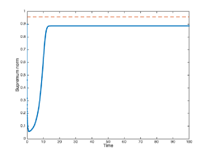
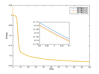
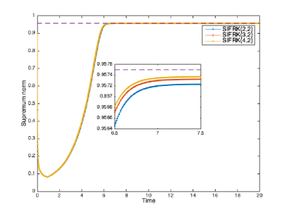
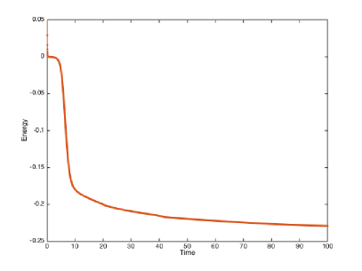
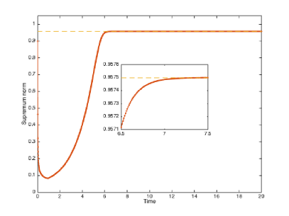
Fig. 1: Evolutions of energies (left) and supremum norms (right) calculated by using sIFRK(1,1) (top), sIFRK($s$,2) (middle) and Heun-sIFRK(3,3) (bottom) schemes with $\tau=0.01$.

We partition the spatial domain by a uniform mesh with the size $h=1/1024$, and a random data ranging from $-0.9$ to $0.9$ is generated on the mesh as the initial configuration. We conduct the simulations by using the proposed sIFRK schemes with the time-step size $\tau=0.01$. Fig. 1 shows the evolutions of the energies and the supremum norms of the approximate solutions. We observe that the energy decreases monotonically and the MBP is preserved perfectly for all of them. However, there is an obvious large gap between the theoretical bound $0.9575$ and the supremum norm of the steady state obtained by sIFRK(1,1). The reason is what we have mentioned in Remark 3, that is, $g_{1}(\kappa\tau)<1$ and the difference is of order $\mathcal{O}((\kappa\tau)^{2})$ as discussed in Section 4.1. This implies that the first-order sIFRK method is practically not accurate although stable when the time-step size $\tau$ is not small enough.

Now, we consider a classic example for simulating a shrinking bubble driven by the Allen-Cahn equation (28) with $\epsilon=0.01$ and

(29) $$f(u)=u-u^{3}$$

subject to the homogeneous Neumann boundary condition. The initial bubble is given by

$$u_{0}(x,y)=\left\{\begin{array}[]{rl}1,&\text{if }x^{2}+y^{2}\leq 0.25^{2},\\ -1,&\text{otherwise},\end{array}\right.$$

and illustrated in Fig. 2.

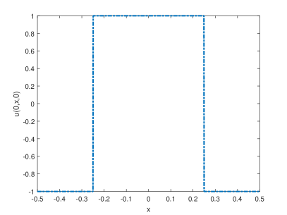
Fig. 2: Initial configuration of the bubble. Left: the surface-project view; right: the cross-section view at $y=0$.

The sIFRK(2,2) scheme is adopted and the parameters of the space-time mesh are set to be $h=1/1024$ and $\tau=0.01$. Fig. 3 presents the evolutions of the bubble at times $t=50$, $100$, $150$, $200$, $250$ and $300$, respectively, and the left graph in Fig. 4 gives the corresponding cross-section views with $y=0$. The right graph in Fig. 4 presents the evolution of the energy, which is monotonically decreasing. The bubble shrinks smaller and smaller during the evolution and finally vanishes at about $t=310$.

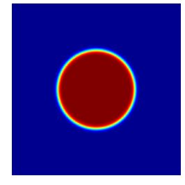
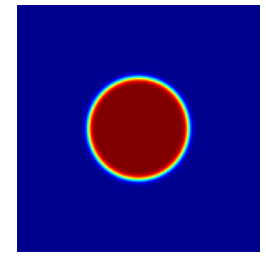
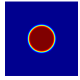
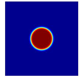
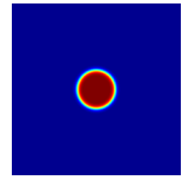
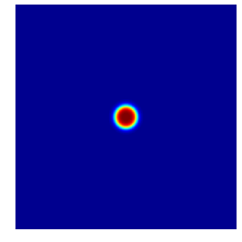
Fig. 3: Evolution of the shrinking bubble obtained by using sIFRK(2,2) with $\tau=0.01$. From left to right and from top to bottom: $t=50$, $100$, $150$, $200$, $250$ and $300$.

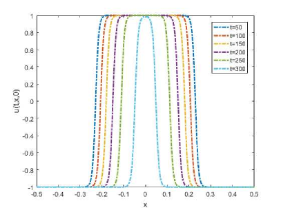
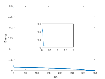
Fig. 4: The cross-section view with $y=0$ (left) corresponding to Fig. 3 and the evolution of the energy (right).

Next, we numerically show that the SSP-sIFRK(2,2) scheme (24) is not unconditionally MBP-preserving in response to the discussion in Remark 6. To this end, we consider the Allen-Cahn equation (28) with $\epsilon=0.01$ and (29) subject to the periodic boundary condition. The initial data is generated by a set of random numbers ranging from $-0.9$ to $0.9$ uniformly on the spatial mesh with $h=1/256$. The time-step size is set to be $\tau=0.1$, which is 10 times larger than that in the previous experiments. We first run the simulation using SSP-sIFRK(2,2) taking the following form

$$u^{(1)} =e^{\tau\mathcal{L}^{h}_{\kappa}}(u^{n}+\tau\mathcal{N}[u^{n}]),$$

$$u^{n+1} =\frac{1}{2}e^{\tau\mathcal{L}^{h}_{\kappa}}u^{n}+\frac{1}{2}(u^{(1)}+\tau\mathcal{N}[u^{(1)}]).$$

Then we re-run the simulation using sIFRK(2,2) with the same initial data. Figs. 5 and 7 present the evolutions of the phase structures at $t=1$, $5$, $10$, $50$, $240$ and $440$ produced by SSP-sIFRK(2,2) and sIFRK(2,2), respectively, which show that the simulation results start to differ very soon although we use the same initial data and space-time parameters. Figs. 6 and 8 present the evolutions of the corresponding supremum norms and the energies for SSP-sIFRK(2,2) and sIFRK(2,2), respectively. It is observed that the MBP is preserved perfectly by sIFRK(2,2) for all time. However, the solution by SSP-sIFRK(2,2) has the supremum norm beyond $1$ after $t=5.5$, which implies SSP-sIFRK(2,2) does not preserve the MBP in this case.

In addition, we carry out the same experiment using sIFRK(2,2), but with different time-step sizes, $\tau=0.05$ and $0.01$. We found that both simulated processes of the phase transition are almost identical to that illustrated in Fig. 7. The corresponding evolutions of the supremum norms and the energies are also given and compared with those produced with $\tau=0.1$ in Fig. 8, which shows very small differences between them. These observations partly imply that the error constant in Theorem 4 does not change much when those different time-step sizes are adopted, and the performance of sIFRK(2,2) is still satisfactory, in terms of accuracy and efficiency, for practical simulations with moderately large time-step sizes.

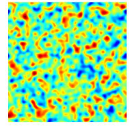
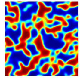
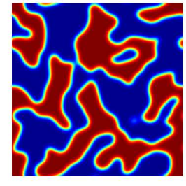
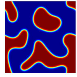
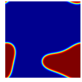
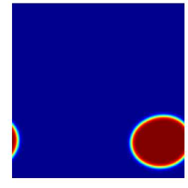
Fig. 5: Evolution of the phase structure obtained by using SSP-sIFRK(2,2) with $\tau=0.1$. From left to right and from top to bottom: $t=1$, $5$, $10$, $50$, $240$ and $440$.

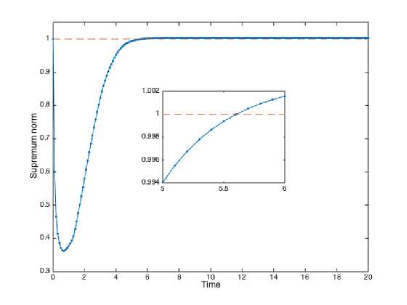
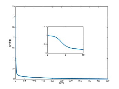
Fig. 6: Evolutions of the supremum norm (left) and the energy (right) obtained by using SSP-sIFRK(2,2) with $\tau=0.1$.

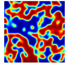
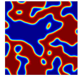
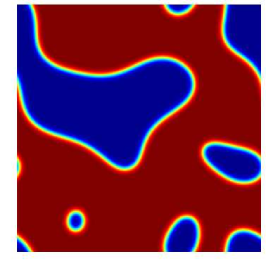
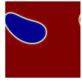
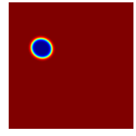
Fig. 7: Evolution of the phase structure obtained by using sIFRK(2,2) with $\tau=0.1$. From left to right and from top to bottom: $t=1$, $5$, $10$, $50$, $240$ and $440$.

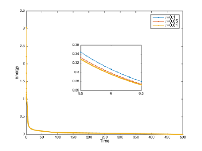
Fig. 8: Evolutions of the supremum norm (left) and the energy (right) obtained by using sIFRK(2,2) with $\tau=0.1$, $0.05$ and $0.01$.

5.3 Three-dimensional simulations

The last experiment is devoted to numerical simulation for the 3D Allen-Cahn equation (28) with $\epsilon=0.01$ and (29). We take the domain $\Omega=(-0.5,0.5)^{3}$ with a uniform spatial mesh of size $h=1/256$, and generate the initial data by the random numbers ranging from $-0.9$ to $0.9$ on the mesh. The sIFRK(2,2) scheme is used for the simulation. Fig. 9 presents the evolutions of the 3D phase structures at $t=1$, $5$, $10$, $50$, $240$ and $350$ with the time-step size $\tau=0.01$, respectively. Fig. 10 plots the evolutions of the supremum norm and the energy of the numerical solutions with different time-step sizes $\tau=0.1$, $0.05$ and $0.01$. The MBP is well-preserved and the energy decreases monotonically along the time as shown in Fig. 10. In addition, we again observe that there are only very small differences between the curves corresponding to different time-step sizes, which implies that sIFRK(2,2) still perform very well for 3D simulations even with moderately large time-step sizes.

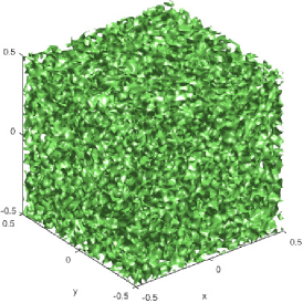
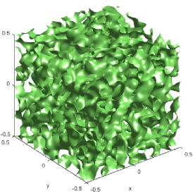
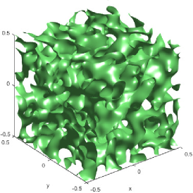
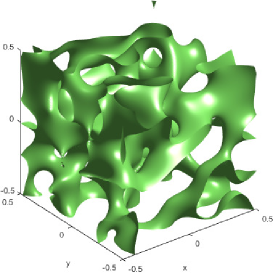
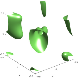
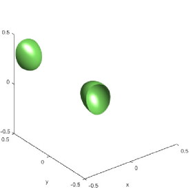
Fig. 9: Evolution of the 3D phase structure obtained by using sIFRK(2,2) with $\tau=0.01$. From left to right and from top to bottom: $t=1$, $5$, $10$, $50$, $240$ and $350$.

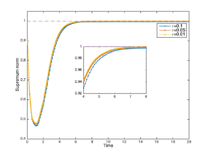
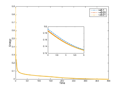
Fig. 10: Evolutions of the supremum norm (left) and the energy (right) of the 3D simulations obtained by using sIFRK(2,2) with $\tau=0.1$, $0.05$ and $0.01$.

6 Conclusion

In this work, we first combine the linear stabilization technique with the IFRK method to develop a family of sIFRK schemes. We derive sufficient conditions to guarantee unconditional preservation of the MBP for the sIFRK method written in different forms. Based on these conditions, we then check various existing IFRK and SSP-IFRK schemes and identify the unconditionally MBP preserving schemes among them, as well as various numerical demonstrations. In addition, we also find that many existing SSP-sIFRK schemes violate these conditions except the first-order one, and thus may not be unconditionally MBP-preserving as verified in numerical experiments.

One important question remains whether the conditions in Theorem 3 or Theorem 5 are also necessary for unconditional MBP preservation, which would be a natural topic for our future research. It is also worth mentioning that Assumption 2 implies that the operator $\mathcal{L}^{h}$ is dissipative. Discretizing $\mathcal{L}$ with the central difference method or the finite element method with mass-lumping satisfies Assumption 2 since the resulting discrete matrix is an $M$-matrix. As we know, the matrix corresponding to the spectral collocation method is usually not an $M$-matrix. Thus another question is whether such assumption is necessary for the space-discrete system to possess the MBP and subsequently for the fully-discrete system.

References

- [1] S. M. Allen and J. W. Cahn, A microscopic theory for antiphase boundary motion and its application to antiphase domain coarsening, Acta Metall., 27 (1979), pp. 1085–1095.
- [2] G. Beylkin, J. M. Keiser, and L. Vozovoi, A new class of time discretization schemes for the solution of nonlinear PDEs, J. Comput. Phys., 147 (1998), pp. 362–387.
- [3] E. Burman and A. Ern, Stabilized Galerkin approximation of convection-diffusion-reaction equations: discrete maximum principle and convergence, Math. Comp., 74 (2005), pp. 1637–1652.
- [4] W. B. Chen, C. Wang, X. M. Wang, and S. M. Wise, Positivity-preserving, energy stable numerical schemes for the Cahn–Hilliard equation with logarithmic potential, J. Comput. Phys.: X, 3 (2019), 100031.
- [5] P. G. Ciarlet, Discrete maximum principle for finite-difference operators, Aequationes Math., 4 (1970), pp. 338–352.
- [6] P. G. Ciarlet and P. A. Raviart, Maximum principle and uniform convergence for the finite element method. Comput. Methods Appl. Mech. Engrg., 2 (1973), pp. 17–31.
- [7] S. M. Cox and P. C. Matthews, Exponential time differencing for stiff systems, J. Comput. phys., 176 (2002), pp. 430–455.
- [8] Q. Du, Nonlocal Modeling, Analysis, and Computation, Vol. 94 of CBMS-NSF regional conference series in Applied Mathematics, SIAM, 2019.
- [9] Q. Du, L. Ju, X. Li, and Z. H. Qiao, Maximum principle preserving exponential time differencing schemes for the nonlocal Allen–Cahn Equation, SIAM J. Numer. Anal., 57 (2019), pp. 875–898.
- [10] Q. Du, L. Ju, X. Li, and Z. H. Qiao, Maximum bound principles for a class of semilinear parabolic equations and exponential time differencing schemes, SIAM Rev., 2020, to appear. (Also available at arXiv:2005.11465)
- [11] Q. Du, L. Ju, and J. F. Lu, Analysis of fully discrete approximations for dissipative systems and application to time-dependent nonlocal diffusion problems, J. Sci. Comput., 78 (2019), pp. 1438–1466.
- [12] K.-J. Engel and R. Nagel, One-Parameter Semigroups for Linear Evolution Equations, Graduate Texts in Mathematics, Vol. 194, Springer-Verlag, New York, 2000.
- [13] L. C. Evans, Partial Differential Equations, American Mathematical Society, Providence, Rhode Island, 2000.
- [14] L. C. Evans, H. M. Soner, and P. E. Souganidis, Phase transitions and generalized motion by mean curvature, Commun. Pure Appl. Math., 45 (1992), pp. 1097–1123.
- [15] X. L. Feng, T. Tang, and J. Yang, Stabilized Crank–Nicolson/Adams–Bashforth schemes for phase field models, East Asian J. Appl. Math., 3 (2013), pp. 59–80.
- [16] X. Fernández-Real and X. Ros-Oton, Boundary regularity for the fractional heat equation, Rev. R. Acad. Cienc. Exactas Fís. Nat. Ser. A Mat., 110 (2016), pp. 49–64.
- [17] L. Ferracina and M. N. Spijker, Step-size restrictions for total-variation-boundedness in general Runge-Kutta procedures, Appl. Numer. Math., 53 (2005), pp. 265–279.
- [18] S. Gottlieb, C.-W. Shu, and E. Tadmor, Strong stability-preserving high-order time discretization methods, SIAM Rev., 43 (2001), pp. 89–112.
- [19] E. Hairer, S. P. Norsett, and G. Wanner, Solving Ordinary Differential Equations I. Nonstiff Problems (2nd ed.), Springer Series in Computational Mathematics, vol. 8, Springer-Verlag Berlin, 1993
- [20] M. Hochbruck and A. Ostermann, Explicit exponential Runge-Kutta methods for semilinear parabolic problems, SIAM J. Numer. Anal., 43 (2005), pp. 1069–1090.
- [21] T. L. Hou and H. T. Leng, Numerical analysis of a stabilized Crank–Nicolson/Adams–Bashforth finite difference scheme for Allen–Cahn equations, Appl. Math. Lett., 102 (2020), 106150.
- [22] T. L. Hou, T. Tang, and J. Yang, Numerical analysis of fully discretized Crank–Nicolson scheme for fractional-in-space Allen–Cahn equations, J. Sci. Comput., 72 (2017), pp. 1214–1231.
- [23] T. L. Hou, D. F. Xiu, and W. Z. Jiang, A new second-order maximum-principle preserving finite difference scheme for Allen–Cahn equations with periodic boundary conditions, Appl. Math. Lett., 104 (2020), 106265.
- [24] W. Hundsdorfer and M. N. Spijker, Boundedness and strong stability of Runge-Kutta methods, Math. Comp., 80 (2011), pp. 863-886.
- [25] L. Isherwood, Z. J. Grant, and S. Gottlieb, Strong stability-preserving integrating factor Runge-Kutta methods, SIAM J. Numer. Anal., 56 (2018), pp. 3276–3307.
- [26] L. Ju, X. Li, Z. H. Qiao, and J. Yang, Maximum bound principle preserving integrating factor Runge-Kutta methods for semilinear parabolic equations, arXiv:2010.12165, 2020.
- [27] L. Ju, X. Li, Z. H. Qiao, and H. Zhang, Energy stability and error estimates of exponential time differencing schemes for the epitaxial growth model without slope selection, Math. Comp., 87 (2018), pp. 1859–1885.
- [28] L. Ju, J. Zhang, and Q. Du, Fast and accurate algorithms for simulating coarsening dynamics of Cahn–Hilliard equations, Comput. Mater. Sci., 108 (2015), pp. 272–282.
- [29] L. Ju, J. Zhang, L. Y. Zhu, and Q. Du, Fast explicit integration factor methods for semilinear parabolic equations, J. Sci. Comput., 62 (2015), pp. 431–455.
- [30] J. D. Lawson, Generalized Runge-Kutta processes for stable systems with large Lipschitz constants, SIAM J. Numer. Anal., 4 (1967), pp. 372–380.
- [31] X. F. Liu and Q. Nie, Compact integration factor methods for complex domains and adaptive mesh refinement, J. Comput. Phys., 229 (2010), pp. 5692–5706.
- [32] Q. Nie, F. Y. Wan, Y. T. Zhang, and X. F. Liu, Compact integration factor methods in high spatial dimensions, J. Comput. Phys., 227 (2008), pp. 5238–5255.
- [33] G. Peng, Z. M. Gao, and X. L. Feng, A stabilized extremum-preserving scheme for nonlinear parabolic equation on polygonal meshes, Int. J. Numer. Meth FL, 90 (2019), pp. 340–356.
- [34] G. Peng, Z. M. Gao, W. J. Yan, and X. L. Feng, A positivity-preserving nonlinear finite volume scheme for radionuclide transport calculations in geological radioactive waste repository, Int. J. Numer. Method. H., 30 (2019), pp. 516–534.
- [35] A. Ralston, Runge-Kutta method with minimum error bounds. Math. Comp., 16 (1962), pp. 431–437.
- [36] W. Rudin, Principles of Mathematical Analysis, Third Edition, McGraw-Hill Book Co., New York, 1976.
- [37] J. Shen, T. Tang, and J. Yang, On the maximum principle preserving schemes for the generalized Allen–Cahn equation, Commun. Math. Sci., 14 (2016), pp. 1517–1534.
- [38] J. Shen and X. F. Yang, Numerical approximations of Allen–Cahn and Cahn–Hilliard equations, Discrete Contin. Dyn. Syst., 28 (2010), pp. 1669–1691.
- [39] C.-W. Shu and S. Osher, Efficient implementation of essentially non-oscillatory shockcapturing schemes, J. Comput. Phys., 77 (1988), pp. 439–471.
- [40] E. Süli and D. F. Mayers, An Introduction to Numerical Analysis, Cambridge University Press, 2003.
- [41] T. Tang and J. Yang, Implicit-explicit scheme for the Allen–Cahn equation preserves the maximum principle, J. Comput. Math., 34 (2016), pp. 471–481.
- [42] R. S. Varga, On a discrete maximum principle. SIAM J. Numer. Anal., 3 (1966), pp. 355–359.
- [43] X. F. Xiao, Z. H. Dai, and X. L. Feng, A positivity preserving characteristic finite element method for solving the transport and convection-diffusion-reaction equations on general surfaces, Comput. Phys. Commun., 247 (2020), 106941.
- [44] X. F. Xiao, X. L. Feng, and Y. N. He, Numerical simulations for the chemotaxis models on surfaces via a novel characteristic finite element method, Comput. Math. Appl., 78 (2019), pp. 20–34.
- [45] C. J. Xu and T. Tang, Stability analysis of large time-stepping methods for epitaxial growth models, SIAM J. Numer. Anal., 44 (2006), pp. 1759–1779.
- [46] X. F. Yang, Error analysis of stabilized semi-implicit method of Allen–Cahn equation. Discrete Contin. Dyn. Syst. B, 11 (2009), 1057–1070.
- [47] L. Y. Zhu, L. Ju, and W. D. Zhao, Fast high-order compact exponential time differencing Runge-Kutta methods for second-order semilinear parabolic equations, J. Sci. Comput., 67 (2016), pp. 1043–1065.