A symmetric hyperbolic formulation of the vacuum Einstein equations in affine-null coordinates

Abstract

We present a symmetric hyperbolic formulation of the Einstein equations in affine-null coordinates. Giannakopoulos et. al. (T. Giannakopoulos, D. Hilditch, and M. Zilhao, Phys. Rev. D 102, 064035 (2020), arXiv:2007.06419 [gr-qc]) recently showed that the most commonly numerically implemented formulations of the Einstein equations in affine-null coordinates (and other single-null coordinate systems) are only weakly–but not strongly–hyperbolic. By making use of the tetrad-based Newman-Penrose formalism, our formulation avoids the hyperbolicity problems of the formulations investigated by Giannakopoulos et. al. We discuss a potential application of our formulation for studying gravitational wave scattering.

I Introduction

Bondi-like coordinate systems have played an important role in understanding gravitational radiation and the structure of future null infinity in asymptotically flat spacetimesBondi (1960); Sachs and Bondi (1962); Bondi et al. (1962). One of the main attractions of using outgoing Bondi-like coordinates is that the Einstein equations near future null infinity take a relatively simple form when one foliates with an outgoing light-sheet. Moreover, the equations of motion have a nested structure, which can be convenient for analyzing the structure of the equations, and numerically solving them. In numerical relativity, outgoing Bondi-like coordinates have found use in Cauchy-characteristic extraction schemes to accurately extract outgoing gravitational waves near future null infinity Tamburino and Winicour (1966); Bishop et al. (1996); Handmer et al. (2016); Winicour (2009). A specific variant of Bondi-like coordinates, ingoing affine-null coordinates, have found extensive use in numerical studies of black hole/black branes in asymptotically anti de Sitter (AdS) spacetimes (for a review, see Chesler and Yaffe (2014)). Ingoing affine-null coordinates have been useful in those contexts as they simplify the study of gravitational radiation near black hole/black brane horizons.

Despite their longtime use, the hyperbolicity properties of the Einstein equations in Bondi-like coordinate systems was only recently studied by Giannakopoulos et. al. Giannakopoulos et al. (2020). Surprisingly, those authors found that the Einstein Equations, when written as an evolution system for the metric in those Bondi and affine-null coordinates, formed only a weakly–but not strongly–hyperbolic system of partial differential equations for the metric components. Following the general approach of Friedrich (1981); Luk (2011); Hilditch et al. (2020), we show that it is relatively straightforward to write down a symmetric (and hence strongly) hyperbolic formulation of the Einstein equations when one works in the tetrad-based based Newman-Penrose Newman and Penrose (1962) formalism. Unfortunately, our symmetric hyperbolic evolution system does not have the same convenient nested structure as the Einstein equations written as an evolution system for the metric components in Bondi-like coordinates. Moreover, working in the Newman-Penrose formalism significantly increases the number of dynamical variables one must solve for. Despite these potential drawbacks, the formulation could have some applications in studying gravitational wave scattering, which we discuss in Secs. IV and V.

Strong hyperbolicity is a necessary condition for system of partial differential equations (PDE) to have a well posed initial value problem for generic initial data Kreiss and Lorenz (1989). Moreover, numerical solutions to a system of PDE can only converge to the continuum solution if the system is well-posed. As not all formulations of the Einstein equations are strongly hyperbolic, any given formulation of the equations must be explicitly checked (for further discussion and review see, e.g. Sarbach and Tiglio (2012); Hilditch (2013)). We review the concepts of weak, strong, and symmetric hyperbolicity in Appendix B.

Compared to work on Bondi-like (or single-null) coordinate systems, there is an extensive literature on the hyperbolicity of the Einstein equations in double null coordinates, which we briefly review. The first major result goes back to FriedrichFriedrich (1981), who showed that the Einstein equations form a strongly hyperbolic system in a tetrad formulation when using double null coordinates. Friedrich further proved a local existence of solutions near the intersection of the two initial characteristic data surfaces. Luk later provided an improved existence result (following earlier work by RendallRendall (1990)) using a tetrad formalismLuk (2011); which was later reformulated in the Newman-Penrose formalism by Hilditch et. al.Hilditch et al. (2020). While we believe that it is likely that our formulation has a well-posed initial value problem, we are unaware of any theorem that demonstrates that strongly hyperbolic single-null formulations of the Einstein equations have a well-posed initial value problem, and it is beyond the scope of this article to provide such a theorem here.

Our sign conventions for the metric, Riemann tensor, etc follow Newman and PenroseNewman and Penrose (1962) (see also ChandrasekharChandrasekhar (2002)); e.g. we use $+---$ signature for the metric. We work in four spacetime dimensions. We index spacetime indices $(0,1,2,3)$ with lower-case Greek letters, and index angular indices $(2,3)$ with lower-case Latin letters. An overbar represent complex conjugation.

II Choice of tetrad for affine-null coordinates

We will use the same tetrad choice as is used in Newman and Penrose (1962)§6. We first write down the metric for outgoing affine-null coordinates (we consider the case of ingoing affine-null coordinates in Appendix A):

$$ds^{2}= Vdu^{2}+2dudr$$

$$-h_{ab}\left(d\theta^{a}+W^{a}du\right)\left(d\theta^{b}+W^{b}du\right).$$ (1)

We have used our four coordinate degrees of freedom to set $g_{rr}=g_{ra}=0$, and $g_{ru}=1$. With these conditions, we see that $u$ is a null coordinate: ($g^{\alpha\beta}\partial_{\alpha}u\partial_{\beta}u=0$). We see with this choice of coordinates that $r$ is an affine parameter for outgoing null geodesics.

As in Newman and Penrose (1962)§6, we choose the following tetrad:

$$l^{\mu}\partial_{\mu}= \partial_{r},$$ (2a)

$$n^{\mu}\partial_{\mu}= \partial_{u}+P\partial_{r}+R^{a}\partial_{a},$$ (2b)

$$m^{\mu}\partial_{\mu}= Q\partial_{r}+S^{a}\partial_{a}.$$ (2c)

where $Q$ and $S^{a}$ are complex. Relating the tetrad to the metric via the identity $g^{\mu\nu}=l^{\mu}n^{\nu}+n^{\mu}l^{\nu}-m^{\mu}\bar{m}^{\nu}-\bar{m}^{\mu}m^{\nu},$ (see Appendix C), we find that

$$g^{rr}=-V= 2\left(P-Q\bar{Q}\right),$$ (3a)

$$g^{ra}=-W^{a}= R^{a}-\bar{S}^{a}Q-S^{a}\bar{Q},$$ (3b)

$$g^{ab}=-h^{ab}= -S^{a}\bar{S}^{b}-S^{b}\bar{S}^{a}.$$ (3c)

The tetrad we have chosen satisfies $\kappa=\mathcal{R}\epsilon=0$. There are three remaining tetrad degrees of freedom, which can be expressed as:

$$n^{\mu}\to n^{\mu},\qquad l^{\mu}\to\bar{z}m^{\mu}+z\bar{m}^{\mu}+z\bar{z}n^{\mu},\qquad m^{\mu}\to m^{\mu}+zn^{\mu},$$

$$n^{\mu}\to n^{\mu},\qquad l^{\mu}\to l^{\mu},\qquad m^{\mu}\to e^{ix}m^{\mu},$$

where $z$ is complex and $x$ is real, which we use to set $\pi=0$ and $\mathcal{I}\epsilon=0$, respectively. To summarize, we have used our six tetrad rotations to set

$$\kappa=\pi=\epsilon=0.$$ (4)

More physically, we have used our six tetrad degrees of freedom to make $l^{\mu}$ geodesic, and to parallel propagate $n^{\mu}$ and $m^{\mu}$ along that geodesic: $l^{\mu}\nabla_{\mu}l^{\nu}=l^{\mu}\nabla_{\mu}n^{\nu}=l^{\mu}\nabla_{\mu}m^{\nu}=0$

III Symmetric hyperbolic formulation of the Einstein equations

In this section we present our symmetric hyperbolic formulation of the Einstein equations, using our coordinates and tetrad from Sec. II. To simplify some of our expressions, we will make use the Geroch-Held-Penrose (GHP) derivative operatorsGeroch et al. (1973) ð, $\textnormal{\dh}^{\prime}$ and $\textnormal{\th}^{\prime}$. As we have set $\epsilon=0$, the operators þ and $D$ are equivalent. We will continue to use $D$ to emphasize the special role the outgoing null vector $l^{\mu}$ plays in this formulation of the Einstein equations.

We obtain evolution equations for the coefficients of $l^{\mu}$ and $m^{\mu}$ by using the tetrad commutation relations (32):

$$Dn^{\mu}+\left(\gamma+\bar{\gamma}\right)l^{\mu}-\bar{\tau}m^{\mu}-\tau\bar{m}^{\mu}= 0,$$ (5a)

$$Dm^{\mu}+\left(\bar{\alpha}+\beta\right)l^{\mu}-\bar{\rho}m^{\mu}-\sigma\bar{m}^{\mu}= 0.$$ (5b)

Eqs. (5) should be read as expressions for the individual components of $l^{\mu}$ and $m^{\mu}$. Writing things out in terms of components, we have

$$DP+\left(\gamma+\bar{\gamma}\right)-\bar{\tau}Q-\tau\bar{Q}= 0,$$ (6a)

$$DR^{a}-\bar{\tau}S^{a}-\tau\bar{S}^{a}= 0,$$ (6b)

$$DQ+\left(\bar{\alpha}+\beta\right)-\bar{\rho}Q-\rho\bar{Q}= 0,$$ (6c)

$$DS^{a}-\bar{\rho}S^{a}-\rho\bar{S}^{a}= 0.$$ (6d)

From the Ricci identities, Eqs. (33), we can write down the following system for the nonzero Ricci rotation coefficients:

$$D\rho-\rho^{2}+\sigma\bar{\sigma}= 0,$$ (7a)

$$D\sigma-\left(\rho+\bar{\rho}\right)\sigma-\Psi_{0}= 0,$$ (7b)

$$D\tau-\rho\tau-\sigma\bar{\tau}-\Psi_{1}= 0,$$ (7c)

$$D\alpha-\rho\alpha-\bar{\sigma}\beta= 0,$$ (7d)

$$D\beta-\sigma\alpha-\bar{\rho}\beta-\Psi_{1}= 0,$$ (7e)

$$D\gamma-\tau\alpha-\bar{\tau}\beta-\Psi_{2}= 0,$$ (7f)

$$D\lambda-\rho\lambda-\bar{\sigma}\mu= 0,$$ (7g)

$$D\mu-\bar{\rho}\mu-\sigma\lambda-\Psi_{2}= 0,$$ (7h)

$$D\nu-\bar{\tau}\mu-\tau\lambda-\Psi_{3}= 0.$$ (7i)

We can rewrite the Bianchi identities to obtain the following evolution system for the Weyl scalars:

$$\left(\textnormal{\th}^{\prime}+\mu\right)\Psi_{0}-\left(\textnormal{\dh}-4\tau\right)\Psi_{1}-3\sigma\Psi_{2} =0,$$ (8a)

$$\left(D+\textnormal{\th}^{\prime}+2\mu-4\rho\right)\Psi_{1}-\left(\textnormal{\dh}-3\tau\right)\Psi_{2}$$

$$-\left(\textnormal{\dh}^{\prime}+\nu\right)\Psi_{0}-2\sigma\Psi_{3} =0,$$ (8b)

$$\left(D+\textnormal{\th}^{\prime}+3\mu-3\rho\right)\Psi_{2}-\left(\textnormal{\dh}-2\tau\right)\Psi_{3}$$

$$-\left(\textnormal{\dh}^{\prime}+2\nu\right)\Psi_{1}+\lambda\Psi_{0}-\sigma\Psi_{4} =0,$$ (8c)

$$\left(D+\textnormal{\th}^{\prime}+4\mu-2\rho\right)\Psi_{3}-\left(\textnormal{\dh}-\tau\right)\Psi_{4}$$

$$-\left(\textnormal{\dh}^{\prime}+3\nu\right)\Psi_{3}+2\lambda\Psi_{1} =0,$$ (8d)

$$\left(D-\rho\right)\Psi_{4}-\textnormal{\dh}^{\prime}\Psi_{3}+3\lambda\Psi_{2} =0.$$ (8e)

We obtained this system by adding together ((34a)+(34f)), ((34b)+(34g)), and ((34c)+(34h)). With this, we see that we have specified a system of evolution/constraint equations for all of the nonzero Newman-Penrose scalars and metric components (via the tetrad components of $n^{\mu}$ and $m^{\mu}$).

To determine the hyperbolicity of the evolution system defined by Eqs. (5), (7), and (8), we write down the principal part:

$$\begin{pmatrix}\mathcal{D}_{1}^{\mu}&0&0\\ 0&\mathcal{D}_{2}^{\mu}&0\\ 0&0&\mathcal{D}_{3}^{\mu}\end{pmatrix}\partial_{\mu}\begin{pmatrix}\vec{\Psi}\\ \vec{\Gamma}\\ \vec{g}\end{pmatrix},$$ (9a)

where

$$\mathcal{D}_{1}^{\mu}\equiv \begin{pmatrix}n^{\mu}&-m^{\mu}&0&0&0\\ -\bar{m}^{\mu}&l^{\mu}+n^{\mu}&-m^{\mu}&0&0\\ 0&-\bar{m}^{\mu}&l^{\mu}+n^{\mu}&-m^{\mu}&0\\ 0&0&-\bar{m}^{\mu}&l^{\mu}+n^{\mu}&-m^{\mu}\\ 0&0&0&-\bar{m}^{\mu}&l^{\mu}\end{pmatrix},$$ (10a)

$$\mathcal{D}_{2}^{\mu}\equiv id_{9}\times l^{\mu},$$ (10b)

$$\mathcal{D}_{3}^{\mu}\equiv id_{8}\times l^{\mu},$$ (10c)

$$\vec{\Psi}^{T}\equiv \left(\Psi_{0},\Psi_{1},\Psi_{2},\Psi_{3},\Psi_{4}\right),$$ (10d)

$$\vec{\Gamma}^{T}\equiv \left(\rho,\sigma,\tau,\alpha,\beta,\gamma,\lambda,\mu,\nu\right),$$ (10e)

$$\vec{g}^{T}\equiv \left(n^{v},n^{r},n^{a},m^{v},m^{r},m^{a}\right),$$ (10f)

($id_{n}$ denotes the $n\times n$ identity matrix). By inspection, we see that the principal symbol

$$\begin{pmatrix}\mathcal{D}_{1}^{\mu}&0&0\\ 0&\mathcal{D}_{2}^{\mu}&0\\ 0&0&\mathcal{D}_{3}^{\mu}\end{pmatrix}\xi_{\mu},$$ (11)

is Hermitian. Moreover, we see that it is positive definite with respect to the timelike direction $t^{\mu}\equiv l^{\mu}+n^{\mu}$:

$$t_{\mu}\begin{pmatrix}\mathcal{D}_{1}^{\mu}&0&0\\ 0&\mathcal{D}_{2}^{\mu}&0\\ 0&0&\mathcal{D}_{3}^{\mu}\end{pmatrix}=\mathrm{diag}\left(1,2,2,2,1,d_{9},d_{8}\right),$$ (12)

where $d_{n}\equiv\mathrm{diag}\left(id_{n}\right)$. We conclude that the evolution system defined by defined by Eqs, (8), (7), and (5) is symmetric hyperbolic with respect to the timelike direction $t^{\mu}$ (c.f. Hilditch et al. (2020) for a similar recent construction, but which instead works in double null coordinates).

IV Incoming gravitational wave initial data

Given that $l^{\mu}\partial_{\mu}=\partial_{r}$, we see that Eqs. (7), (5) form a system of “constraint” equations for the Ricci rotation coefficients and tetrad components along a $u=const.$ hypersurface. Using the Bianchi identities (34a)-(34d), we can write down a system of constraint equations for the Weyl scalars $\Psi_{1},\Psi_{2},\Psi_{3}$, and $\Psi_{4}$:

$$\left(D-4\rho\right)\Psi_{1}-\textnormal{\dh}^{\prime}\Psi_{0} =0,$$ (13a)

$$\left(D-3\rho\right)\Psi_{2}-\textnormal{\dh}^{\prime}\Psi_{1}+\lambda\Psi_{0} =0,$$ (13b)

$$\left(D-2\rho\right)\Psi_{3}-\textnormal{\dh}^{\prime}\Psi_{2}+2\lambda\Psi_{1} =0,$$ (13c)

$$\left(D-\rho\right)\Psi_{4}-\textnormal{\dh}^{\prime}\Psi_{3}+3\lambda\Psi_{1} =0.$$ (13d)

Given these equations, provided we have constraint satisfying initial data at $r=r_{min}$ on our $u=u_{i}$ initial data surface, the only free initial data left to specify are the real and imaginary components of $\Psi_{0}$. The remaining technical challenge with this initial data setup is to find consistent initial data for the constrained variables at the point $r=r_{min}$ of our initial data surface. One simple prescription is to have all of the Newman-Penrose scalars satisfy a known, exact solution to the Einstein equations at $r=r_{min}$: $\alpha=\alpha^{(bkgrd)},\Psi_{4}=\Psi_{4}^{(bkgrd)}$, etc. Then, over a compact region (in $r$) on the $u=u_{i}$ initial data surface, one sets

$$\Psi_{0}={}^{(bkgrd)}\Psi_{0}+{}^{+}\Psi_{0},$$ (14)

where ${}^{(bkgrd)}\Psi_{0}$ is the known, “background” solution to $\Psi_{0}$, and ${}^{+}\Psi_{0}$ is the free initial specification of $\Psi_{0}$. We can think of ${}^{+}\Psi_{0}$ as specifying an incoming gravitational wave added on top of a given exact solution to the Einstein equations. Given the exact background solution, we have consistent initial data at $r=r_{min}$, and we can then use the constraint equations Eqs. (7), (5), and (13) to specify consistent initial data over the entire $u=const.$ hypersurface. As we evolve in time, we must continue to specify consistent boundary data at $r=r_{min}$. For all time before the “packet” of ${}^{+}\Psi_{0}$ reaches that boundary, we can continue to set all of the Newman-Penrose scalars to their background values at that boundary. After that point, one would need to specify evolution equations for the other Newman-Penrose scalars on the boundary to continue to have consistent boundary data there.

We conclude that in this particular setup we have specified purely ingoing gravitational wave initial data, with no outgoing gravitational waves at the boundary $r=r_{min}$ (provided the background solution is stationary). See Fig. 1 for a schematic illustration.

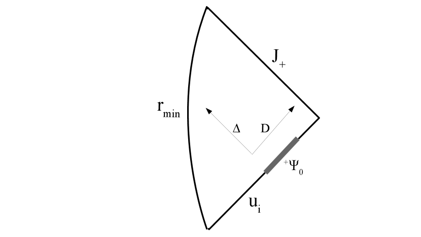
Figure 1: Schematic Penrose diagram for purely ingoing gravitational radiation initial data. On the initial $u=u_{i}$ initial data surface, one specifies ${}^{+}\Psi_{0}$ over a compact region. All of the other Ricci rotation coefficients, Weyl scalars, and metric components can then be found on the initial data surface by integrating their respective evolution/constraint equations. At the boundary $r=r_{min}$ all Newman-Penrose scalars are set to be their “background” values; this is consistent initial data for the times before the “packet” of ${}^{+}\Psi_{0}$ reaches that boundary. See Sec. IV for more discussion.

V Discussion

While single-null coordinates provide several conceptual and technical advantages over Cauchy-like evolution schemes, the most commonly used formulations of the Einstein equations in those coordinate systems were recently shown to be only weakly –but not strongly–hyperbolic Giannakopoulos et al. (2020). We have shown that by using the tetrad-based Newman-Penrose formalism, it is relatively straightforward to construct a symmetric hyperbolic formulation of the Einstein equations in affine-null coordinates, which are example of a single null (or Bondi-like) coordinate system. We have also presented a method to construct purely ingoing gravitational wave initial data, which could be used to analytically and/or numerically study gravitational wave scattering problems. While we have only considered outgoing affine-null coordinates (II), our formulation can be straightforwardly adapted to ingoing affine-null coordinates by applying the GHP “prime” operatorGeroch et al. (1973) to all of our equations; see Appendix A for more details.

As strong hyperbolicity is a necessary property for the well-posedness of the initial value formulation of a PDE, the condition is widely regarded as a crucial property a system of PDE must have in order for that system to be amenable to stable numerical evolution, (see, e.g. Sarbach and Tiglio (2012); Hilditch (2013)). This being said, numerical evolution of weakly hyperbolic systems may only give non-convergent/pathological results with initial data that is sufficiently “rough”, and at sufficiently high numerical resolution Giannakopoulos et al. (2020). The stable, convergent evolution of many numerical schemes that have used single-null (and weakly hyperbolic) formulations of the Einstein equations could potentially be explained by the fact that those earlier studies worked with smooth initial data, and use numerical dissipation (which is typically required for stable numerical evolution of even strongly hyperbolic systems, see, e.g. Gustafsson et al. (1995)).

While we have derived a strongly hyperbolic formulation of the Einstein equations, we have not proven that that system has a well posed initial value problem. While Rendall Rendall (1990) and Luk Luk (2011) have provided general theorems that demonstrate local existence of solutions for strongly hyperbolic formulations of double null formulations of the Einstein equations, we work with a single-null formulation, and thus their results are not directly applicable to our formulation. We leave to future work a suitable generalization of their results to single-null strongly hyperbolic systems.

We caution that from a practical standpoint we have not considered other important qualities a system of PDE must satisfy in order to admit stable numerical evolution. For example, we have not analyzed the stability of “constraint violating modes” in the evolution system, whose potential growth away from the constraint surface could effectively rule out practical any numerical evolution of the system (for more discussion, see, e.g. Brodbeck et al. (1999); Gundlach et al. (2005)). More generally, we have not computed any bound on the region for which a solution to the system we have presented would have well-posed evolution off of the initial data hypersurface. Studying the domain of existence of solutions could be studied using the techniques used by the authors of, e.g. Hilditch et al. (2020).

In this article we have only provided a prescription for initial data that involves an ingoing gravitational wave (although in Appendix A we discuss how one could set up outgoing gravitational wave initial data when working in ingoing affine-null coordinates). We restricted ourselves to that kind of initial data due to the form of the evolution/constraint Eqs. (5), (7), and (13): with that system we could use the real and imaginary parts of $\Psi_{0}$ as free initial data, provided we had constraint satisfying initial data at the boundary $r=r_{min}$ of our initial data ($u=const.$) surface. The most straightforward way of satisfying this constraint is by setting the boundary to be a known solution to the Einstein equations. A more detailed analysis of the Newman-Penrose equations may reveal a better/more generic way of providing constraint equations at $r=r_{min}$. While we leave constructing more sophisticated initial data sets in this formulation to future work, we note that already the initial data setup we provide could allow for investigations of gravitational wave scattering to future null infinity (for the outgoing null coordinates considered in the body of this article), or the scattering of gravitational wave scattering into black holes (for the ingoing null coordinates considered in Appendix A).

We have only considered a symmetric hyperbolic formulation of one kind of single-null coordinate system, namely affine-null coordinates. More general single null coordinates can be written as

$$ds^{2}= Ve^{2B}du^{2}+2e^{2B}dudr$$

$$-h_{ab}\left(d\theta^{a}+W^{a}du\right)\left(d\theta^{b}+W^{b}du\right),$$ (15)

where we have introduced the function $B(u,r,\theta^{a})$ (c.f. Giannakopoulos et al. (2020)). This form of the metric captures a wide variety of single-null coordinate systems, e.g. when $B=0$ we recover affine-null coordinates, and when $\mathrm{det}h_{ab}=r^{2}\mathrm{det}s_{ab}$, where $s_{ab}$ is the metric of the unit two-sphere, we recover the classical Bondi-Sachs coordinates. We leave to future work the construction of strongly hyperbolic formulations of the Einstein equations for this more general set of single-null coordinates.

Data availability

Data sharing is not applicable to this article as no new data were created or analyzed in this study.

Appendix A A symmetric hyperbolic formulation of the Einstein equations in ingoing affine-null coordinates

For completeness, here we present a symmetric hyperbolic formulation of the Einstein equations in ingoing affine-null coordinates:

$$ds^{2}= Vdv^{2}-2dvdr$$

$$-h_{ab}\left(d\theta^{a}+W^{a}dv\right)\left(d\theta^{b}+W^{b}dv\right).$$ (16)

Here $v$ is the null coordinate for ingoing null hypersurfaces. While outgoing affine-null coordinates are specially adapted to outgoing gravitational radiation, ingoing affine-null coordinates find most of their use in studies of black hole/black brane horizons. For example, ingoing affine-null coordinates have been widely used in numerical simulations of asymptotically AdS spacetimes that contain black holes/black branes Chesler and Yaffe (2014).

We choose the following tetrad

$$n^{\mu}\partial_{\mu}= -\partial_{r},$$ (17a)

$$l^{\mu}\partial_{\mu}= \partial_{v}+P\partial_{r}+R^{a}\partial_{a},$$ (17b)

$$m^{\mu}\partial_{\mu}= Q\partial_{r}+S^{a}\partial_{a}.$$ (17c)

where $Q$ and $S^{a}$ are complex. We use the six tetrad degrees of freedom to set

$$\nu=\tau=\gamma=0.$$ (18)

In other words, we use our six tetrad degrees of freedom to make $n^{\mu}$ geodesic, and to parallel propagate $l^{\mu}$ and $m^{\mu}$ along that geodesic: $n^{\mu}\nabla_{\mu}n^{\nu}=n^{\mu}\nabla_{\mu}l^{\nu}=n^{\mu}\nabla_{\mu}m^{\nu}=0.$ We can find the coefficients for $l^{\mu}$ and $m^{\mu}$ by using the commutation relations(32):

$$\Delta l^{\mu}-\left(\epsilon+\bar{\epsilon}\right)n^{\mu}+\pi m^{\mu}+\bar{\pi}\bar{m}^{\mu}= 0,$$ (19a)

$$\Delta m^{\mu}-\left(\bar{\alpha}+\beta\right)n^{\mu}+\mu m^{\mu}+\bar{\lambda}\bar{m}^{\mu}= 0.$$ (19b)

Writing Eq. (19) in terms of tetrad components, we have

$$DP+\left(\epsilon+\bar{\epsilon}\right)+\pi Q+\bar{\pi}\bar{Q}= 0,$$ (20a)

$$DR^{a}+\pi S^{a}+\bar{\pi}\bar{S}^{a}= 0,$$ (20b)

$$DQ+\left(\bar{\alpha}+\beta\right)+\mu Q+\bar{\lambda}\bar{Q}= 0,$$ (20c)

$$DS^{a}+\mu S^{a}+\bar{\lambda}\bar{S}^{a}= 0.$$ (20d)

From the Ricci rotation identities (33), we obtain the following evolution equations for the nonzero Ricci rotation coefficients

$$\Delta\lambda+\left(\mu+\bar{\mu}\right)\lambda+\Psi_{4}= 0,$$ (21a)

$$\Delta\mu+\mu^{2}+\lambda\bar{\lambda}= 0,$$ (21b)

$$\Delta\pi+\mu\pi+\lambda\bar{\pi}+\Psi_{3}= 0,$$ (21c)

$$\Delta\rho+\bar{\mu}\rho+\sigma\lambda+\Psi_{2}= 0,$$ (21d)

$$\Delta\sigma+\mu\sigma+\bar{\lambda}\rho= 0,$$ (21e)

$$\Delta\kappa+\bar{\pi}\rho+\pi\sigma+\Psi_{1}= 0,$$ (21f)

$$\Delta\alpha+\bar{\mu}\alpha+\lambda\beta+\Psi_{3}= 0,$$ (21g)

$$\Delta\beta+\mu\beta+\bar{\lambda}\alpha= 0,$$ (21h)

$$\Delta\epsilon+\bar{\pi}\alpha+\pi\beta+\Psi_{2}= 0.$$ (21i)

We rewrite the Bianchi identities to obtain the following evolution system for the Weyl scalars:

$$\left(\Delta+\mu\right)\Psi_{0}-\textnormal{\dh}\Psi_{1}-3\sigma\Psi_{2} =0,$$ (22a)

$$\left(\Delta+\textnormal{\th}+2\mu-4\rho\right)\Psi_{1}-\left(\textnormal{\dh}-3\kappa\right)\Psi_{2}$$

$$-\left(\textnormal{\dh}^{\prime}+\pi\right)\Psi_{0}-2\sigma\Psi_{3} =0,$$ (22b)

$$\left(\Delta+\textnormal{\th}+3\mu-3\rho\right)\Psi_{2}-\left(\textnormal{\dh}-2\kappa\right)\Psi_{3}$$

$$-\left(\textnormal{\dh}^{\prime}+2\pi\right)\Psi_{1}+\lambda\Psi_{0}-\sigma\Psi_{4} =0,$$ (22c)

$$\left(\Delta+\textnormal{\th}+4\mu-2\rho\right)\Psi_{3}-\left(\textnormal{\dh}-\kappa\right)\Psi_{4}$$

$$-\left(\textnormal{\dh}^{\prime}+3\pi\right)\Psi_{2}+2\lambda\Psi_{1} =0,$$ (22d)

$$\left(\textnormal{\th}-\rho\right)\Psi_{4}-\left(\textnormal{\dh}^{\prime}+4\pi\right)\Psi_{3}+3\lambda\Psi_{2} =0.$$ (22e)

As in Sec. III, we obtained this system by adding together ((34a)+(34f)), ((34b)+(34g)), and ((34c)+(34h)).

Similarly to what we did in Sec. IV we can specify initial data by setting all the Newman-Penrose scalar to be equal to some exact, background solution at $r=r_{max}$ on the $v=v_{i}$ initial hypersurface. We can then construct outgoing radiation on that slice by freely specifying the real and imaginary parts of ${}^{+}\Psi_{4}$, and then integrating inwards in $r$ from $r=r_{max}$ the following constraint equations for the Weyl scalars (which are taken from the Bianchi identities 34e-34h)

$$\left(\Delta+\mu\right)\Psi_{0}-\textnormal{\dh}\Psi_{1}-3\sigma\Psi_{2}= 0,$$ (23a)

$$\left(\Delta+2\mu\right)\Psi_{1}-\textnormal{\dh}\Psi_{2}-2\sigma\Psi_{3}= 0,$$ (23b)

$$\left(\Delta+3\mu\right)\Psi_{2}-\textnormal{\dh}\Psi_{3}-\sigma\Psi_{4}= 0,$$ (23c)

$$\left(\Delta+4\mu\right)\Psi_{3}-\textnormal{\dh}\Psi_{4}= 0.$$ (23d)

the tetrad components, and the Ricci rotation coefficients from their equations of motion Eqs. (19) and (21), respectively. To evolve in time, we could set all the Newman-Penrose scalars to be equal to their background value at $r=r_{max}$, and specify $\Psi_{4}={}^{(bkgrd)}\Psi_{4}+{}^{+}\Psi_{4}$, where ${}^{+}\Psi_{4}$ is specified over a compact region of the initial data surface. One potential advantage of the ingoing formulation is that if we compactify in $r$ to spatial infinity, then our boundary data at spatial infinity will always be consistent. With regards to what happens at the origin ($r=0$), typically ingoing affine-null coordinates are used to study black hole/black brane spacetimes, and in those cases the domain only needs to extend to the black hole horizon (for more discussion see e.g. Chesler and Yaffe (2014)).

Appendix B A brief review of weak, strong, and symmetric hyperbolic systems

For completeness, we review the notions of weak, strong, and symmetric hyperbolic systems; for a more in-depth account see, e.g. Kreiss and Lorenz (1989); Sarbach and Tiglio (2012); Hilditch (2013). We begin with a system of evolution PDE of the form

$$\hat{A}\partial_{t}{\bf u}+\hat{B}^{i}\left(t,{\bf x},{\bf u}\right)\partial_{i}{\bf u}+{\bf F}\left(t,{\bf x},{\bf u}\right)=0,$$ (24)

where ${\bf u}$ is the state vector, $\partial_{i}\equiv\partial/\partial x^{i}$, and we sum over the indices $i$. The system (24) is weakly hyperbolic if the principal symbol

$$\mathcal{P}\left(\xi\right)\equiv\hat{A}^{-1}\hat{B}^{i}\xi_{i}$$ (25)

has all real eigenvalues for all unit spatial vectors $\xi_{i}$. It is strongly hyperbolic if for every unit spatial vector $\xi_{i}$ the principal symbol has a complete set of eigenvectors, and that there exists a constant $K$ independent of $\xi_{i}$ such that

$$\left|\hat{T}_{\xi}\right|+\left|\hat{T}^{-1}_{\xi}\right|\leq K,$$ (26)

where the columns of the matrix $\hat{T}_{\xi}$ are given by the eigenvectors of $\mathcal{P}\left(\xi\right)$. The system (24) is symmetric hyperbolic if there is a Hermitian positive definite symmetrizer $H$ such that $HA^{i}\xi_{i}$ is Hermitian for every unit spatial vector $\xi_{i}$. Symmetric hyperbolicity implies strong hyperbolicity, and strong hyperbolicity implies weak hyperbolicity, but the converse of these statements do not hold.

In this article we consider systems of PDE that take the slightly more general form

$$\hat{A}^{\mu}\left(t,{\bf x},{\bf u}\right)\partial_{\mu}{\bf u}+{\bf F}\left(t,{\bf x},{\bf u}\right)=0,$$ (27)

where $x^{\mu}$ ranges over space and time. If there is a timelike vector $t^{\mu}$ such that then the matrix

$$\hat{A}^{\mu}t_{\mu},$$ (28)

is positive definite, we can then perform a coordinate transform to make (27) take the more classical form (24) (in particular, transform coordinates so that $t_{\mu}=\delta^{0}_{\mu}$; then $\hat{A}\equiv\hat{A}^{0}$, and $\hat{B}^{i}\equiv\hat{A}^{i}$ in the new coordinate system). We conclude that in order to show that systems of PDE that take the form (27) are symmetric hyperbolic, it is sufficient to show that $\hat{A}^{\mu}\xi_{\mu}$ is Hermitian for all $\xi_{\mu}$, and that there is a timelike vector $t^{\mu}$ such that $\hat{A}^{\mu}t_{\mu}$ is positive definite.

Appendix C The Newman-Penrose and Geroch-Held-Penrose formalisms

The Newman-Penrose Newman and Penrose (1962) and Geroch-Held-Penrose Geroch et al. (1973) are tetrad based reformulations of the Einstein equations. For reference, we list the main Newman-Penrose equations that we use in this article. We note that we only consider the vacuum Einstein equations, which in terms of the metric form the following system of equations:

$$R_{\mu\nu}=0,$$ (29)

where $R_{\mu\nu}$ is the Ricci tensor. For a more complete description of the Newman-Penrose and Geroch-Held-Penrose formalisms, see Newman and Penrose (1962); Geroch et al. (1973); Chandrasekhar (2002); our notation follows Newman and PenroseNewman and Penrose (1962) (see also ChandrasekharChandrasekhar (2002)). As is standard, we denote the null tetrad as $n^{\mu},l^{\mu},m^{\mu}$, where $m^{\mu}$ is a complex null vector, $n^{\mu}$ is an ingoing null vector, and $l^{\mu}$ is an outgoing null vector. The metric then is

$$g_{\mu\nu}=n_{\mu}l_{\nu}+l_{\mu}n_{\nu}-m_{\mu}\bar{m}_{\nu}-\bar{m}_{\mu}m_{\nu}.$$ (30)

The derivative operators are

$$D\equiv l^{\mu}\partial_{\mu},\qquad\Delta\equiv n^{\mu}\partial_{\mu},\qquad\delta\equiv m^{\mu}\partial_{\mu}.$$ (31)

The derivative commutation relations are

$$\Delta D-D\Delta= \left(\gamma+\bar{\gamma}\right)D+\left(\epsilon+\bar{\epsilon}\right)\Delta-\left(\bar{\tau}+\pi\right)\delta-\left(\tau+\bar{\pi}\right)\bar{\delta},$$ (32a)

$$\Delta D-D\delta= \left(\bar{\alpha}+\beta-\bar{\pi}\right)D+\kappa\Delta-\left(\bar{\rho}+\epsilon-\bar{\epsilon}\right)\delta-\sigma\bar{\delta},$$ (32b)

$$\delta\Delta-\Delta\delta= -\bar{\nu}D+\left(\tau-\bar{\alpha}-\beta\right)\Delta+\left(\mu-\gamma+\bar{\gamma}\right)\delta+\bar{\lambda}\bar{\delta},$$ (32c)

$$\bar{\delta}\delta-\delta\bar{\delta}= \left(\bar{\mu}-\mu\right)D+\left(\bar{\rho}-\rho\right)\Delta+\left(\alpha-\bar{\beta}\right)\delta+\left(\beta-\bar{\alpha}\right)\bar{\delta}.$$ (32d)

The vacuum Ricci rotation identities are

$${D}\rho-\bar{{\delta}}\kappa =(\rho^{2}+\sigma\bar{\sigma})+\rho(\epsilon+\bar{\epsilon})-\bar{\kappa}\tau-\kappa(3\alpha+\bar{\beta}-\pi),$$ (33a)

$${D}\sigma-{\delta}\kappa =\sigma(\rho+\bar{\rho}+3\epsilon-\bar{\epsilon})-\kappa(\tau-\bar{\pi}+\bar{\alpha}+3\beta)+\Psi_{0}$$ (33b)

$${D}\tau-{\Delta}\kappa =\rho(\tau+\bar{\pi})+\sigma(\bar{\tau}+\pi)+\tau(\epsilon-\bar{\epsilon})-\kappa(3\gamma+\bar{\gamma})+\Psi_{1}$$ (33c)

$${D}\alpha-\bar{{\delta}}\epsilon =\alpha(\rho+\bar{\epsilon}-2\epsilon)+\beta\bar{\sigma}-\bar{\beta}\epsilon-\kappa\lambda-\bar{\kappa}\gamma+\pi(\epsilon+\rho)$$ (33d)

$${D}\beta-{\delta}\epsilon =\sigma(\alpha+\pi)+\beta(\bar{\rho}-\bar{\epsilon})-\kappa(\mu+\gamma)-\epsilon(\bar{\alpha}-\bar{\pi})+\Psi_{1}$$ (33e)

$${D}\gamma-{\Delta}\epsilon =\alpha(\tau+\bar{\pi})+\beta(\bar{\tau}+\pi)-\gamma(\epsilon+\bar{\epsilon})-\epsilon(\gamma+\bar{\gamma})+\tau\pi-\nu\kappa+\Psi_{2}$$ (33f)

$${D}\lambda-\bar{{\delta}}\pi =(\rho\lambda+\bar{\sigma}\mu)+\pi(\pi+\alpha-\bar{\beta})-\nu\bar{\kappa}-\lambda(3\epsilon-\bar{\epsilon})$$ (33g)

$${D}\mu-{\delta}\pi =(\bar{\rho}\mu+\sigma\lambda)+\pi(\bar{\pi}-\bar{\alpha}+\beta)-\mu(\epsilon+\bar{\epsilon})-\nu\kappa+\Psi_{2}$$ (33h)

$${D}\nu-{\Delta}\pi =\mu(\pi+\bar{\tau})+\lambda(\bar{\pi}+\tau)+\pi(\gamma-\bar{\gamma})-\nu(3\epsilon+\bar{\epsilon})+\Psi_{3}$$ (33i)

$${\Delta}\lambda-\bar{{\delta}}\nu =-\lambda(\mu+\bar{\mu}+3\gamma-\bar{\gamma})+\nu(3\alpha+\bar{\beta}+\pi-\bar{\tau})-\Psi_{4}$$ (33j)

$${\delta}\rho-\bar{{\delta}}\sigma =\rho(\bar{\alpha}+\beta)-\sigma(3\alpha-\bar{\beta})+\tau(\rho-\bar{\rho})+\kappa(\mu-\bar{\mu})-\Psi_{1}$$ (33k)

$${\delta}\alpha-\bar{{\delta}}\beta =\mu\rho-\lambda\sigma+\alpha\bar{\alpha}+\beta\bar{\beta}-2\alpha\beta+\gamma(\rho-\bar{\rho})+\epsilon(\mu-\bar{\mu})-\Psi_{2}$$ (33l)

$${\delta}\lambda-\bar{{\delta}}\mu =\nu(\rho-\bar{\rho})+\pi(\mu-\bar{\mu})+\mu(\alpha+\bar{\beta})+\lambda(\bar{\alpha}-3\beta)-\Psi_{3}$$ (33m)

$${\delta}\nu-{\Delta}\mu =(\mu^{2}+\lambda\bar{\lambda})+\mu(\gamma+\bar{\gamma})-\bar{\nu}\pi+\nu(\tau-3\beta-\bar{\alpha})$$ (33n)

$${\delta}\gamma-{\Delta}\beta =\gamma(\tau-\bar{\alpha}-\beta)+\mu\tau-\sigma\nu-\epsilon\bar{\nu}-\beta(\gamma-\bar{\gamma}-\mu)+\alpha\bar{\lambda}$$ (33o)

$${\delta}\tau-{\Delta}\sigma =(\mu\sigma+\bar{\lambda}\rho)+\tau(\tau+\beta-\bar{\alpha})-\sigma(3\gamma-\bar{\gamma})-\kappa\bar{\nu}$$ (33p)

$${\Delta}\rho-\bar{{\delta}}\tau =-\rho\bar{\mu}+\sigma\lambda+\tau(\bar{\beta}-\alpha-\bar{\tau})+\rho(\gamma+\bar{\gamma})+\nu\kappa-\Psi_{2}$$ (33q)

$${\Delta}\alpha-\bar{{\delta}}\gamma =\nu(\rho+\epsilon)-\lambda(\tau+\beta)+\alpha(\bar{\gamma}-\bar{\mu})+\gamma(\bar{\beta}-\bar{\tau})-\Psi_{3}$$ (33r)

The vacuum Bianchi identities are

$$-\bar{{\delta}}\Psi_{0}+{D}\Psi_{1}+(4\alpha-\pi)\Psi_{0}-2(2\rho+\epsilon)\Psi_{1}+3\kappa\Psi_{2}+ =0,$$ (34a)

$$\bar{{\delta}}\Psi_{1}-{D}\Psi_{2}-\lambda\Psi_{0}+2(\pi-\alpha)\Psi_{1}+3\rho\Psi_{2}-2\kappa\Psi_{3} =0,$$ (34b)

$$-\bar{{\delta}}\Psi_{2}+{D}\Psi_{3}+2\lambda\Psi_{1}-3\pi\Psi_{2}+2(\epsilon-\rho)\Psi_{3}+\kappa\Psi_{4}+ =0,$$ (34c)

$$\bar{{\delta}}\Psi_{3}-{D}\Psi_{4}-3\lambda\Psi_{2}+2(2\pi+\alpha)\Psi_{3}-(4\epsilon-\rho)\Psi_{4} =0,$$ (34d)

$$-{\Delta}\Psi_{0}+{\delta}\Psi_{1}+(4\gamma-\mu)\Psi_{0}-2(2\tau+\beta)\Psi_{1}+3\sigma\Psi_{2} =0,$$ (34e)

$$-{\Delta}\Psi_{1}+{\delta}\Psi_{2}+\nu\Psi_{0}+2(\gamma-\mu)\Psi_{1}-3\tau\Psi_{2}+2\sigma\Psi_{3} =0,$$ (34f)

$$-{\Delta}\Psi_{2}+{\delta}\Psi_{3}+2\nu\Psi_{1}-3\mu\Psi_{2}+2(\beta-\tau)\Psi_{3}+\sigma\Psi_{4} =0,$$ (34g)

$$-{\Delta}\Psi_{3}+{\delta}\Psi_{4}+3\nu\Psi_{2}-2(\gamma+2\mu)\Psi_{3}-(\tau-4\beta)\Psi_{4} =0,$$ (34h)

Geroch, Held, and Penrose Geroch et al. (1973) showed that the derivative operators $D,\Delta,\delta$, when acting on the Newman-Penrose scalars are generically not invariant under tetrad rotations. They classified scalars $f$ as having weights $(p,q)$ if under the rescaling (here $c$ is a complex field) $l^{\mu}\to c\bar{c}l^{\mu}$, $n^{\mu}\to c^{-1}\bar{c}^{-1}n^{\mu}$, $m^{\mu}\to c\bar{c}^{-1}m^{\mu}$, it transforms as $f\to c^{p}\bar{c}^{q}f$. For a scalar field $f$ of weight $(p,q)$, they defined the following tetrad rotation covariant operators

$$\textnormal{\th}f\equiv\left(D-p\epsilon-q\bar{\epsilon}\right)f,\qquad\textnormal{\th}^{\prime}f\equiv\left(\Delta-p\gamma-q\bar{\gamma}\right)f,\qquad\textnormal{\dh}f\equiv\left(\delta-p\beta-q\bar{\alpha}\right)f,\qquad\textnormal{\dh}^{\prime}f\equiv\left(\bar{\delta}-p\alpha-q\bar{\beta}\right)f.$$ (35)

References

- Bondi (1960) H. Bondi, Nature 186, 535 (1960).
- Sachs and Bondi (1962) R. K. . Sachs and H. Bondi, Proceedings of the Royal Society of London. Series A. Mathematical and Physical Sciences 270, 103 (1962), https://royalsocietypublishing.org/doi/pdf/10.1098/rspa.1962.0206 .
- Bondi et al. (1962) H. Bondi, M. G. J. Van der Burg, and A. W. K. Metzner, Proceedings of the Royal Society of London. Series A. Mathematical and Physical Sciences 269, 21 (1962), https://royalsocietypublishing.org/doi/pdf/10.1098/rspa.1962.0161 .
- Tamburino and Winicour (1966) L. A. Tamburino and J. H. Winicour, Phys. Rev. 150, 1039 (1966).
- Bishop et al. (1996) N. T. Bishop, R. Gomez, L. Lehner, and J. Winicour, Phys. Rev. D 54, 6153 (1996), arXiv:gr-qc/9705033 .
- Handmer et al. (2016) C. J. Handmer, B. Szilágyi, and J. Winicour, Class. Quant. Grav. 33, 225007 (2016), arXiv:1605.04332 [gr-qc] .
- Winicour (2009) J. Winicour, Living Rev. Rel. 12, 3 (2009), arXiv:0810.1903 [gr-qc] .
- Chesler and Yaffe (2014) P. M. Chesler and L. G. Yaffe, JHEP 07, 086 (2014), arXiv:1309.1439 [hep-th] .
- Giannakopoulos et al. (2020) T. Giannakopoulos, D. Hilditch, and M. Zilhao, Phys. Rev. D 102, 064035 (2020), arXiv:2007.06419 [gr-qc] .
- Friedrich (1981) H. Friedrich, Proceedings of the Royal Society of London. A. Mathematical and Physical Sciences 375, 169 (1981), https://royalsocietypublishing.org/doi/pdf/10.1098/rspa.1981.0045 .
- Luk (2011) J. Luk, (2011), arXiv:1107.0898 [gr-qc] .
- Hilditch et al. (2020) D. Hilditch, J. A. Valiente Kroon, and P. Zhao, Gen. Rel. Grav. 52, 99 (2020), arXiv:1911.00047 [gr-qc] .
- Newman and Penrose (1962) E. Newman and R. Penrose, Journal of Mathematical Physics 3, 566 (1962).
- Note (1) We note that the possibility of a strongly hyperbolic formulation of the Einstein equations for Bondi-like coordinate systems existing for a tetrad-based formalism was suggested by Giannakopoulos et. al. Giannakopoulos et al. (2020).
- Kreiss and Lorenz (1989) H. Kreiss and J. Lorenz, Initial-Boundary Value Problems and the Navier-Stokes Equations, ISSN (Elsevier Science, 1989).
- Note (2) As is stressed in Giannakopoulos et al. (2020) though, this does not imply that a numerical solution of a weakly hyperbolic system will necessarily exhibit any pathological behavior at a given fixed resolution.
- Sarbach and Tiglio (2012) O. Sarbach and M. Tiglio, Living Rev. Rel. 15, 9 (2012), arXiv:1203.6443 [gr-qc] .
- Hilditch (2013) D. Hilditch, Int. J. Mod. Phys. A 28, 1340015 (2013), arXiv:1309.2012 [gr-qc] .
- Rendall (1990) A. D. Rendall, Proceedings of the Royal Society of London. A. Mathematical and Physical Sciences 427, 221 (1990), https://royalsocietypublishing.org/doi/pdf/10.1098/rspa.1990.0009 .
- Note (3) For a review which discusses earlier attempts to formulate a well-posed initial value problem for single-null formulations of the Einstein equations, see Winicour (2009).
- Chandrasekhar (2002) S. Chandrasekhar, The mathematical theory of black holes, Oxford classic texts in the physical sciences (Oxford Univ. Press, Oxford, 2002).
- Geroch et al. (1973) R. Geroch, A. Held, and R. Penrose, Journal of Mathematical Physics 14, 874 (1973), https://doi.org/10.1063/1.1666410 .
- Gustafsson et al. (1995) B. Gustafsson, H. Kreiss, and J. Oliger, Time Dependent Problems and Difference Methods, A Wiley-Interscience Publication (Wiley, 1995).
- Brodbeck et al. (1999) O. Brodbeck, S. Frittelli, P. Hübner, and O. A. Reula, Journal of Mathematical Physics 40, 909 (1999), https://doi.org/10.1063/1.532694 .
- Gundlach et al. (2005) C. Gundlach, J. M. Martin-Garcia, G. Calabrese, and I. Hinder, Class. Quant. Grav. 22, 3767 (2005), arXiv:gr-qc/0504114 .
- Note (4) For example, this is done in Hilditch et al. (2020). In their case it is more straightforward to do this as with their tetrad condition the derivatives only involve “angular” derivatives, so the Newman-Penrose equations (33k\@@italiccorr)-(33m\@@italiccorr) provide a convenient set of constraint equation at the .