A Survey on Fundamental Limits of Integrated Sensing and Communication

Abstract

The integrated sensing and communication (ISAC), in which the sensing and communication share the same frequency band and hardware, has emerged as a key technology in future wireless systems due to two main reasons. First, many important application scenarios in fifth generation (5G) and beyond, such as autonomous vehicles, Wi-Fi sensing and extended reality, requires both high-performance sensing and wireless communications. Second, with millimeter wave and massive multiple-input multiple-output (MIMO) technologies widely employed in 5G and beyond, the future communication signals tend to have high-resolution in both time and angular domain, opening up the possibility for ISAC. As such, ISAC has attracted tremendous research interest and attentions in both academia and industry. Early works on ISAC have been focused on the design, analysis and optimization of practical ISAC technologies for various ISAC systems. While this line of works are necessary, it is equally important to study the fundamental limits of ISAC in order to understand the gap between the current state-of-the-art technologies and the performance limits, and provide useful insights and guidance for the development of better ISAC technologies that can approach the performance limits. In this paper, we aim to provide a comprehensive survey for the current research progress on the fundamental limits of ISAC. Particularly, we first propose a systematic classification method for both traditional radio sensing (such as radar sensing and wireless localization) and ISAC so that they can be naturally incorporated into a unified framework. Then we summarize the major performance metrics and bounds used in sensing, communications and ISAC, respectively. After that, we present the current research progresses on fundamental limits of each class of the traditional sensing and ISAC systems. Finally, the open problems and future research directions are discussed.

I Introduction

Future beyond 5G and sixth generation (6G) wireless systems are expected to provide various high-accuracy sensing services, such as indoor localization for robot navigation, Wi-Fi sensing for smart home and radar sensing for autonomous vehicles. Sensing and communication systems are usually designed separately and occupy different frequency bands. However, due to the wide deployment of the millimeter wave and massive MIMO technologies, communication signals in future wireless systems tend to have high-resolution in both time and angular domain, making it possible to enable high-accuracy sensing using communication signals. As such, it is desirable to jointly design the sensing and communication systems such that they can share the same frequency band and hardware to improve the spectrum efficiency and reduce the hardware cost. This motivates the study of integrated sensing and communication (ISAC). It is believed that ISAC will become a key technology in future wireless systems to support many important application scenarios [1, 2, 3, 4, 5]. For example, in future autonomous vehicle networks, the autonomous vehicles will obtain a large amount of information from the network, including ultra-high resolution maps and near real-time information to help navigate and avoid upcoming traffic congestion [6]. In the same scenario, radar sensing in the autonomous vehicles should be able to provide robust, high-resolution obstacle detection on the order of a centimeter [7]. The ISAC technology for autonomous vehicles provides the potential to achieve both high-data rate communications and high-resolution obstacle detection using the same hardware and spectrum resource. Other applications of ISAC include Wi-Fi based indoor localization and activity recognition, unmanned aerial vehicle (UAV) communication and sensing, extended reality (XR), joint radar (target tracking and imaging) and communication systems etc. Each application has different requirements, limits, and regulatory issues. Fig. 1 illustrates some possible application areas for ISAC.

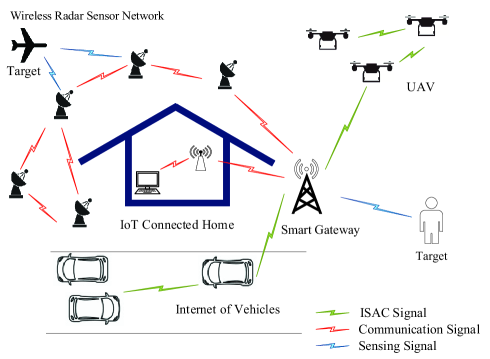
Figure 1: Illustration for the applications of ISAC.

Under this background, ISAC has attracted tremendous research interest and attentions in both academia and industry. For example, recently, there have been an increasing number of academic publications on ISAC, ranging from transceiver architecture and frame structure [3, 8], ISAC waveform design [9, 10, 11], joint coding design [12, 13, 14], temporal-spectral-spatial signal processing [15, 16, 17], to experimental performance demonstrations, prototyping, and field-tests [18]. The authors of this paper have also organized IEEE WTC Special Interest Group (SIG) on ISAC and a workshop on ISAC in IEEE Global Communications Conference in 2020. Furthermore, in September and November 2019, IEEE 802.11 formed the WLAN Sensing Topic Interest Group and Study Group, respectively, and formed a new official Task Group IEEE 802.11bf in September 2020, with the objective of incorporating wireless sensing as a new feature for next-generation WiFi systems (e.g., Wi-Fi 7).

Despite these early research efforts on ISAC, many important problems about ISAC remain open, such as the unified theoretical frameworks, the fundamental performance limits, and the optimal ISAC schemes and signal processing algorithms. In particular, characterizing the fundamental limits of ISAC, including the distortion bounds for sensing parameters (such as the direction of arrival (DOA), signal propagation time delay, Doppler frequency, position, velocity etc.) as well as the channel capacity and capacity-distortion tradeoff performance, is of great importance to make breakthrough in ISAC technologies. On one hand, the fundamental limits provide a performance bound for practical ISAC technologies, which reveals the potential gap between the current technologies and the optimal solution. On the other hand, the fundamental limits analysis also provides useful guidance and insight for the design and analysis of practical ISAC systems. Recently, a number of works have been dedicated to studying the fundamental limits of ISAC, see e.g., [19, 20]. However, many important questions remain open and need further study. In this paper, we conduct a comprehensive survey on the fundamental limits of various sensing systems and ISAC systems, and discuss the open problems and potential research directions. We hope that this survey serves as a starting point for interested researchers to work on this important and challenging research area.

Some related works are reviewed below. There are many survey papers for traditional sensing technologies, including radar sensing [21], wireless localization [22, 23, 24, 25], WiFi and mobile sensing [26, 27, 28], among which only a few works have discussed the fundamental limits of traditional sensing. For example, the fundamental limits of radar sensing and wireless localization have been surveyed in [21] and [22], respectively. Recently, several works have also presented the recent research progress on joint radar and communication (JRC) system, which can be viewed as a special case of ISAC considered in this paper. In [1], the authors presented the applications, topologies, levels of system integration, the current state of the art, and outlines of future information-centric JRC systems. In [3], the authors overviewed the application scenarios and research progress in radar-communication coexistence and dual-functional radar-communication systems. In [29], the author first reviewed the work on coexisting communication and radar systems, then provided a brief review for three types of JRC systems and finally reviewed stimulating research problems and potential solutions. However, previous works such as [1], [3] and [29] mainly focus on the design, analysis and optimization of practical JRC systems, and there still lacks a comprehensive survey on the fundamental limits of ISAC. To summarize, a number of contributions differentiate this paper from existing works:

• We propose a systematic classification method for both traditional radio sensing technologies (such as radar sensing and wireless localization) and ISAC technologies so that they can be naturally incorporated into a unified framework.

• Existing survey works on ISAC mainly focus on the joint system design and integration, but pay little attention to the fundamental limits of the integrated system. To our best of knowledge, this is the first work to provide a comprehensive survey on the fundamental limits of both radio sensing and ISAC systems.

• We propose several typical ISAC channel topologies as abstracted models for various ISAC systems, analogous to traditional communication channel topologies. We point out that the fundamental limits of ISAC channels cannot be obtained by a trivial combinations of existing performance bounding techniques in separate sensing and communication systems.

• We present a list of important open challenges and potential research directions on ISAC, many of which have not been mentioned in the previous works.

The rest of the paper is organized as follows. Section II describes the classifications of integrated sensing and communication. Section III presents some essential performance metrics for radio sensing as well as integrated sensing and communication. Sections IV - VII present the current research progress on the fundamental limits of the device-free sensing, device-based sensing, device-free ISAC, and device-based ISAC, respectively. Section VIII discusses open problems and future research directions in ISAC. Finally, we make our conclusions in Section IX.

II Classifications of Integrated Sensing and Communication

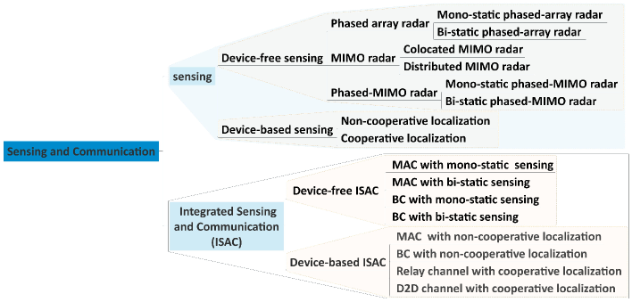
Figure 2: An overview of classifications of ISAC.

Traditional radio sensing can be classified into two categories, namely, the device-free sensing and device-based sensing.

• Device-free sensing means that the sensing targets (e.g., a bird) are not capable of transmitting and/or receiving the sensing signal, or means that the sensing procedure does not rely on the transmitting and/or receiving of the sensing target (e.g., a target vehicle). A typical example for device-free sensing is the radar sensing.

• Device-based sensing means that the sensing targets are capable of transmitting and/or receiving the sensing signal, and the sensing procedure relies on the transmitting and/or receiving of the sensing target. A typical example is the wireless-based localization to localize mobile devices.

Naturally, ISAC can also be classified into device-free ISAC and device-based ISAC as it will be illustrated later. In this section, we first briefly discuss the history of device-free and device-based sensing/ISAC. Then we provide a detailed classifications for each category, which are also summarized in Fig. 2.

In terms of device-free sensing, the earliest radar can be traced back to 1904 [30]. In 1950, the concept of phased-array radar first appeared. Through decades of development, the concept of MIMO radar is introduced in 2004 [31] and the concept of phased-MIMO radar was proposed in 2010 [32]. As an attempt to integrate the radar and communication, the concept of joint radar-communications (JRC) was proposed in 2006 [33]. In terms of device-based sensing, Global Navigation Satellite System (GNSS) has been used to provide location services initially. Owing to the poor performance of the GNSS in indoor environments, the cellular-based localization was proposed as a good alternative to GNSS. The first cellular-based localization system is called E-911 used for providing emergency services [34]. Starting from the second generation (2G), wireless localization has been included as a compulsory feature in the standardization and implementation of cellular networks, with continuous enhancement on the localization accuracy over each generation, e.g., from hundreds of meters accuracy in 2G to tens of meters in the fourth generation (4G). Nowadays, sub meter-level localization accuracy can even be achieved in 5G by state-of-the-art techniques, e.g. millimeter wave and massive MIMO. However, the limited spectrum resource and hardware infrastructure will eventually become a bottleneck for localization. Furthermore, due to the fact that radio signals can simultaneously carry data and location-related information of the transmitters, a unified study on integrated localization and communication (ILAC) tends to be a natural choice. In this paper, integrated sensing and communication (ISAC) is proposed as a more general concept including both the JRC and ILAC as special cases, since they can be viewed as the device-free ISAC and device-based ISAC, respectively.

II-A Device-free Sensing

Since the majority of device-free sensing belong to radar sensing, we will focus on the detailed classifications of radar sensing in this subsection. As illustrated in Fig. 3, radar transmits an omnidirectional or directional probing signal towards the target. Then the probing signal is reflected by the target and the radar echo is received by radar. Finally, the target parameters can be estimated from the received echo.

Generally speaking, there are three radar system architectures: phased-array radar, MIMO radar and phased-MIMO radar. In this subsection, we will further divide these three kinds of radar into different classes and discuss the structure and characteristic of each class.

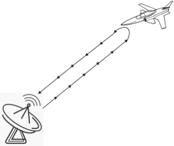
Figure 3: Remote radar sensing of a single target.

II-A1 Phased-array Radar

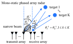
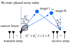
Figure 4: An illustration of different classes of phased-array radar.

Phased-array antennas have been an enabling technology for many systems in support of a variety of radar missions. Phased-array radar employs many antennas placed together respectively for the transmit and receive arrays. The spacing between the antennas within an array is set in the same order of the wavelength of the sensing signal. Each of the transmit antennas transmits a same baseband signal and transmit beamforming is employed to steer a high-gain beam in a particular direction [35].

As illustrated in Fig. 4, phased-array radar can be divided into two classes according to whether the transmit and receive arrays are placed together: mono-static phased-array radar and bi-static phased-array radar.

Mono-static phased-array radar employs a system in which the transmit and receive arrays are placed together. In many cases, the same antenna array is exploited for both transmitting and receiving. In this paper, we slightly extend this concept to include radar systems where the transmit and receive antenna arrays are co-located. The advantage of this kind of placement is that the AoD (angle of departure) and AoA (angle of arrival) are the same in this case, thus fewer parameters need to be estimated. However, the interference from the transmit array to the receive array is non-negligible and needs to be eliminated. One common method for interference elimination is to use pulsed waveforms so that the transmit and the receive functions are performed at different time intervals to avoid interference.

Bi-static phased-array radar employs a system in which the transmit and receive arrays are placed in different sites. Since the AoD and AoA are different in this case, more parameters need to be estimated. However, the interference from the transmit array to the receive array is smaller due to the larger distance.

II-A2 MIMO Radar

MIMO radar was first proposed in [31]. Contrary to the phased-array radar, MIMO radar transmits decorrelated probing signals from independent transmitters. Since independent signals undergo independent fading, MIMO radar can overcome target Radar Cross Section (RCS) scintillations [31]. Moreover, the received signal in MIMO radar is a superposition of independently faded signals, and thus the average SNR of the received signal is more or less constant [31].

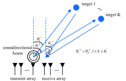
Figure 5: An illustration of colocated MIMO radar.

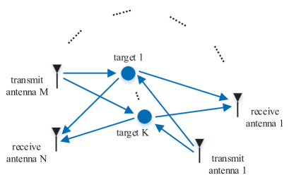
Figure 6: An illustration of distributed MIMO radar.

MIMO radar can be divided into two classes: colocated MIMO radar and distributed MIMO radar [31].

In colocated MIMO radar, the antennas in the transmit or receive antenna array are placed together, and the spacing between the antennas within an array is set in the same order of the signal wavelength, as illustrated in Fig. 5. Note that although the antenna placement of colocated MIMO radar is similar to that of the phased-array radar, the transmit signals are fundamentally different in these two radars, i.e., independent signals in MIMO radar versus beamformed signals in phased-array radar, as explained above. With decorrelated signals transmitted from different transmitters and received by different receivers placed together, the target has been observed multiple times from the same direction, and each observation is independent from each other. In this way, the waveform diversity gain can be achieved to enhance the radar sensing performance [36, 37, 38].

In distributed MIMO radar, the antennas in the transmit or receive antenna array are widely distributed in different locations, and the spacing between any two antennas is far larger than the wavelength, as illustrated in Fig. 6. With independent signals transmitted from distributed transmitters and received by distributed receivers, the target has been observed multiple times from different directions. Hence, the spatial diversity gain can be achieved to increase the accuracy of localization [39, 40, 41]. Note that there is no mono-static distributed MIMO radar since the antennas in both transmit and receive arrays are distributed in the space. However, each node might implement both transmit and receive functions.

II-A3 Phased-MIMO Radar

Phased-MIMO Radar was first proposed in [42] and it achieves a tradeoff between phased-array radar (beamforming gain) and MIMO radar (waveform diversity gain). As illustrated in Fig. 7, the transmit array of phased-MIMO radar is divided into different sub-arrays which are allowed to have overlapping. Each subarray is composed of any number of antennas ranging from 1 to $M$, and forms a beam towards a certain direction. Different waveforms are transmitted by different subarrays. Therefore, each subarray can be regarded as a phased-array radar and all subarrays can be jointly regarded as a MIMO radar. There is no specific limitation imposed on the receive array, but a colocated receive array is typically used [42]. As illustrated in Fig. 7, phased-MIMO radars can be further divided into mono-static phased-MIMO radars and bi-static phased-MIMO radars according to whether the transmit and receive arrays are placed together.

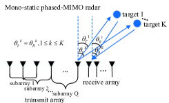
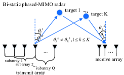
Figure 7: Phased-MIMO radar.

II-A4 Other Device-free Sensing Scenarios

There are some other device-free sensing scenarios that do not necessarily fall into the above classes. For example, passive radar is another technique for device-free sensing which has been investigated for several decades, especially for defence applications [43]. This kind of radar is not intended to send radar probing signals actively. It instead parasitically exploits the echoes from the targets that are illuminated by pre-existing transmitters, being intrinsically bistatic. Various communication transmitters might be employed as illuminators of opportunity thus enabling different applications. Radio and television broadcast transmitters are usually preferred for long range surveillance applications. On the other hand, WiFi access points might be employed for local area monitoring [44, 45]. The passive radar can estimate the desired parameters of the target from the passively received signals. Passive radar has received renewed interest for surveillance purposes because it allows target detection and localization with advantages such as low cost, covert operation, no frequency allocation requirement, etc. However, the sensing performance of the passive radar is totally subject to the communication component. Consequently, its performance is very sensitive to the characteristics of the received waveforms, which may vary significantly over time depending on the requirements and the characteristics of the communication signals and channel. Therefore, advanced methodologies and signal processing techniques have to be implemented to improve the reliability of the resulting sensor against this time-varying scenario [46].

II-B Device-based Sensing

For device-based sensing, we will focus on the wireless-based localization. Though different localization systems exist, e.g., GNSS, localization systems based on WLAN or cellular networks as shown in Fig. 8, they all aim to estimate the location of the targeting object based on a set of wireless reference signals propagated between the reference nodes and the targeting object. The targeting objects with unknown locations are often referred to as agent nodes, and the reference nodes with known locations are often called anchor nodes. In most cases, the agent receives reference signals from the anchors to localizes itself. However, there are also cases in which the anchors receive reference signals from the agents to localize the agents. In this case, if the agent wants to obtain its own position, the anchors will send the estimated position to the agent via a communication link. In this paper, unless otherwise specified, we will mostly focus on the case when the target want to localize itself based on the signals received from multiple anchors. The localization problems in wireless networks can be classified into two classes, namely, cooperative localization and non-cooperative localization. With cooperation among neighboring agent nodes, higher localization accuracy can be achieved, which reveals a different fundamental limits compared to the non-cooperative localization, as will be elaborated below.

Figure 8: Wireless-based localization systems.

II-B1 Non-Cooperative Localization

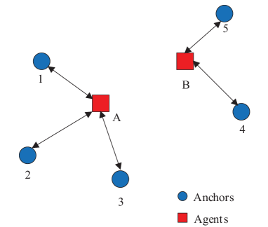
Figure 9: Non-Cooperative Localization.

Consider a non-cooperative localization network with $N_{a}$ agents and $N_{b}$ anchors, where each agent localizes itself based on signals transmitted from neighboring anchors only. Fig. 9 illustrates a special case when $N_{a}=2$, $N_{b}=5$. Agent A receives reference signals from Anchor 1, 2 and 3, while Agent B receives reference signals from Anchor 4 and 5. The position of the agent can be inferred from different metrics of the received signal, including time of arrival (TOA), angle of arrival (AOA), angle of departure (AOD), time difference of arrival (TDOA) and received signal strength (RSS), as detailed below.

TOA or TDOA-based localization method extracts time-based metric from received signals for localization. Generally speaking, TOA-based method estimates the distance by multiplying the signal propagation delay with the light speed. Then, based on trilateration relationship, the agent position can be estimated. TOA-based method requires time synchronization between the agent and all the anchors, which is quite difficult to achieve in practical systems. To overcome this challenge, the TDOA-based method, which only measures the differences in the TOAs from several anchors, is proposed to get rid of the requirement on the time synchronization between the agent and the anchors. In this case, the relative distance is estimated in contrast to the TOA-based absolute distances estimation.

AOA-based localization is another commonly used approach that uses the angles (AOA/AOD) between anchors and the agent node to achieve localization. The angle-based metric can be extracted by an array of antennas. Based on the AOA measurements, the agent can be localized by two anchors in a 2D plane theoretically.

The RSS measurements can also be used for localization. RSS-based localization method neither requires time synchronization among different nodes nor relies on the LOS signal propagation. However, this method has a fatal drawback, namely the poor localization accuracy. This is because the RSS measurements highly rely on the characteristic of the propagation environment. When the environment is harsh, e.g., in destructive shadowing, the localization performance will degrade severely.

It is also possible to combine the above metrics to further enhance the localization performance by using a hybrid method, e.g., based on both TOA and AOA. Nonetheless, in real-life scenario, high-accuracy localization may not be guaranteed by non-cooperative localization owning to limited anchor deployment, especially in harsh environments. For example, some agents may not receive strong signals from a sufficient number of anchors. In this case, it is important to consider cooperative localization which also utilizes signals from other agents, as elaborated below.

II-B2 Cooperative Localization

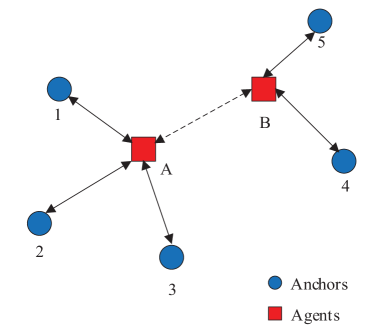
Figure 10: Cooperative localization.

In cooperative localization networks, each agent localizes itself based on measurements from both anchors and other agents. Specifically, as shown in Fig. 10, the agents (A and B) receive signals from the anchors (1, 2, 3, 4 and 5). Agent A is not in the ranging range of Anchor 4 and 5, while Agent B is not in the ranging range of Anchor 1, 2 and 3. Conventionally, each agent needs at least three anchors to accurately localizes itself based on range measurements in a 2-D plane. Therefore, Agent B cannot be well localized if it only receives localization signals from two neighboring anchors. However, if we allow cooperation between Agent A and B, it is possible for Agent B to localizes itself by also using the cooperative localization signals from Agent A. Furthermore, the spatial cooperation mentioned above can be extended to spatio-temporal cooperation, where each agent can incorporate localization information both from other agents (spatial cooperation) and its own localization result in the previous time slot (temporal cooperation).

Based on cooperative localization, higher coverage and accuracy can be achieved with the same number of anchors as the non-cooperative case. The drawback is that in cooperation localization, agents require for stronger signal processing ability and their location may be exposed to other agents.

II-B3 Other Device-based Sensing Scenarios

Apart from wireless localization scenarios mentioned above, many other device-based sensing scenarios have been considered, e.g., fingerprinting-based localization, proximity-based localization and visible light-based positioning (VLP) [47, 48, 49, 50, 51, 52, 53]. In fingerprinting-based localization, unique geotagged signatures, i.e. fingerprints, are extracted from the data collected by the sensors firstly. Then the agent can be localized by matching the online signal measurements against the pre-recorded fingerprints. For fingerprint-based localization, the fingerprints extracted from the signal measurements usually correspond to the RSS, because RSS based metric does not rely on the LOS assumption and performs better in harsh environment. Compared with geometric-based localization, fingerprinting-based localization is more robust to clutter environment. However, its offline training is time-consuming and complex. In proximity-based localization, the position of the anchor which has the strongest RSS is treated as the position of the agent node. Obviously, high location accuracy cannot be guaranteed by this method. VLP is a promising localization method based on transmitting visible light signals, and it has attracted increasing attention from industry and academia recently [54, 55, 56]. However, VLP has severe performance degradation in NLOS case and heavily relies on special equipment.

II-C Device-free ISAC

Device-free ISAC means that in the integrated system, the sensing functionality is achieved by device-free sensing. Device-free ISAC can be categorized according to different ISAC channel topologies. In the following, we discuss several typical device-free ISAC channel topologies, some of which (or simplified versions) have been introduced in [1]. In all these channels, there are one base station (BS), $K$ targets and $U$ users.

II-C1 Multiple Access Channel with Mono-Static Sensing

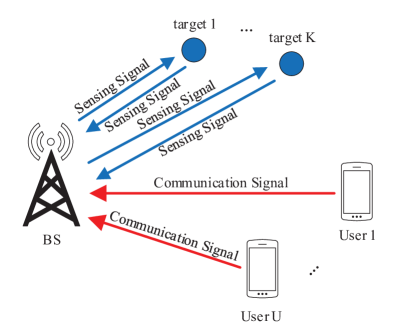
Figure 11: Multiple access channel with mono-static BS sensing.

The multiple access channel (MAC) with mono-static sensing refers to a device-free ISAC channel whose communication channel topology is MAC and radar structure is mono-static (i.e., colocated radar transmitter and receiver). In general, both the BS and mobile users can act as the mono-static radar. Two important special cases include the MAC with mono-static BS sensing in which only the BS acts as a mono-static radar, and the MAC with mono-static mobile sensing in which only the mobile users act as mono-static radars.

Specifically, a MAC with mono-static BS sensing is illustrated in Fig. 11, where the BS acts as both radar transceiver and communication receiver, while the mobile user is a communication transmitter. The BS aims to estimate the relevant parameters of targets and decode the uplink messages from the users. The challenge is that the uplink signals collide with the probing radar echoes at the BS, leading to a joint estimation and decoding problem.

II-C2 Multiple Access Channel with Bi-Static Sensing

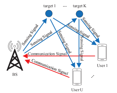
Figure 12: Multiple access channel with bi-static mobile sensing.

The MAC with bi-static sensing refers to a device-free ISAC channel whose communication channel topology is MAC and radar structure is bi-static (i.e., separate radar transmitter and receiver). In general, both the BS and mobile users can act as the bi-static radar sensor (radar receiver). Two important special cases include the MAC with bi-static BS sensing in which only the BS acts as the radar sensor, and the MAC with bi-static mobile sensing in which only the mobile users act as bi-static radar sensors.

Specifically, a MAC with bi-static mobile sensing is illustrated in Fig. 12, where the BS acts as both radar transmitter and communication receiver, while the user acts as both radar receiver and communication transmitter. The users aim to estimate the relevant parameters of the targets while the BS aims to decode the uplink messages from the users. In this case, the processing of uplink signals and the probing radar echoes are decoupled if we do not consider the self-interference at the BS and user sides. A probable circumstance is that the targets are part of the scatters for the communication channels. In this case, the user can acquire partial Channel State information (CSI) from the probing radar echoes. The challenge is how to use this partial Channel State Information (CSI) for better uplink communication.

II-C3 Broadcast Channel with Mono-Static Sensing

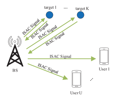
Figure 13: Broadcast channel with mono-static BS sensing.

The broadcast channel (BC) with mono-static sensing refers to a device-free ISAC channel whose communication channel topology is BC and radar structure is mono-static. In general, both the BS and mobile users can act as the mono-static radar. Two important special cases include the BC with mono-static BS sensing in which only the BS acts as a mono-static radar, and the BC with mono-static mobile sensing in which only the mobile users act as mono-static radars.

Specifically, a BC with mono-static BS sensing is illustrated in Fig. 13, where the BS acts as both radar transceiver and communication transmitter, while each user is a downlink communication receiver. In general, a joint transmit waveform can be used for both radar sensing and downlink communications. The BS aims to estimate the relevant parameters of targets while the users aim to decode the downlink messages. In this case, the processing of downlink signals and the probing radar echoes are decoupled since the BS knows the transmit data. The challenge is the joint design of the transmit waveform for both the downlink signals and the probing radar signals at the BS.

II-C4 Broadcast Channel with Bi-static Sensing

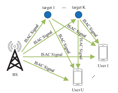
Figure 14: Broadcast channel with Bi-static mobile sensing.

The BC with bi-static sensing refers to a device-free ISAC channel whose communication channel topology is BC and radar structure is bi-static. In general, both the BS and mobile users can act as the bi-static radar sensor (radar receiver). Two important special cases include the BC with bi-static BS sensing in which only the BS acts as a bi-static radar sensor, and the BC with bi-static mobile sensing in which only the mobile users act as bi-static radar sensors.

Specifically, a BC with bi-static mobile sensing is illustrated in Fig. 14, the BS acts as both radar and communication transmitter, while the user acts as both radar and communication receiver. The users aim to estimate the relevant parameters of targets and decode the downlink messages. In this case, the processing of downlink signals and the probing radar echoes are coupled. The user needs to jointly estimate the target parameters and decode the downlink message. The challenges are how to design the joint transmit waveform at the BS and how to handle the superposition of the downlink signals and the probing radar signals at the users.

Note that in the above descriptions, we have focused on cellular network where we call the communication transmitter in the BC or communication receiver in the MAC as the BS. However, the above device-free ISAC channel topologies can also be used to model more general ISAC scenarios. For example, in a general ISAC scenario, we may rename the “MAC with mono-static BS sensing” as “MAC with mono-static Com-Rx sensing” since in this case, the communication receiver serves as the mono-static radar sensor. Similarly, in a general ISAC scenario, we may rename the “BC with mono-static BS sensing” as “BC with mono-static Com-Tx sensing” since in this case, the communication transmitter serves as a mono-static radar sensor.

II-D Device-based ISAC

Device-based ISAC means that in the integrated system, the sensing functionality is achieved by device-based sensing. Device-based ISAC can also be categorized according to different ISAC channel topologies. In the following, we discuss several typical device-based ISAC channel topologies.

II-D1 Multiple Access Channel with Non-Cooperative Localization

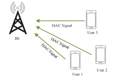
Figure 15: Multiple access channel with non-cooperative localization.

In the multiple access channel with non-cooperative localization illustrated in Fig. 15, the users are going to be localized or communicate with the BS. The BS receives both communication and localization signals from the users and perform joint localization and decoding.

II-D2 Broadcast Channel with Non-Cooperative Localization

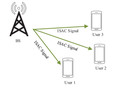
Figure 16: Broadcast channel with non-cooperative localization.

In the broadcast channel with non-cooperative localization illustrated in Fig. 16, the BS transmits a shared waveform to receivers for both localization and communications. Each user needs to eliminate interference from others and extract localization information from the common signals independently. So the role of joint waveform design at the BS is highlighted, which has a huge impact on the performance of both localization and communication.

II-D3 Relay Channel with Cooperative Localization

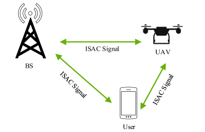
Figure 17: Relay channel with cooperative localization.

In the relay channel with cooperative localization illustrated in Fig. 17, relays such as unmanned aerial vehicles (UAVs) are used to aid both communications and localization. For example, the UAV relay can be located by the ground BSs and then be used as a new anchor node to assist the terrestrial localization. In the meanwhile, the UAV-aided relaying can also provide communication services.

II-D4 D2D Channel with Cooperative Localization

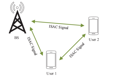
Figure 18: D2D channel with cooperative localization.

In the D2D channel with cooperative localization illustrated in Fig. 18, each user receives signals both from the BS and other neighboring users for communications and localization. Therefore, from communication perspective, there is a D2D communication link providing a direct connection between users. From the localization perspective, there is a cooperative localization link in addition to the anchor-agent link.

III Performance Metrics

In this section, we present the key performance metrics that are useful to characterize the fundamental limits of sensing, communication and ISAC systems. In particular, for sensing systems, estimation-theoretic metrics are considered, while for communication systems, information-theoretic framework and metrics are considered. Both estimation-theoretic and information-theoretic metrics are considered for ISAC systems.

III-A Estimation-Theoretic Metrics for Sensing

The task of sensing is to obtain awareness of the scene surrounding the sensor in general, which includes the capability to detect, localize and track objects, to form images and/or to extract features for recognition/classification purposes, etc. The focus of this paper is to investigate the performance bounds in terms of parameter estimation capability, since many important sensing objectives such as the localization and tracking of objects can be interpreted as parameter estimation problems, and the capability to estimate some key parameters, such as the time delay, DOA, and Doppler frequency, also provides a foundation for more complicated sensing objectives such as recognition and classification.

III-A1 Mean-Square-Error and Relevant Lower Bounds

Let $\boldsymbol{\theta}$ be the true parameter vector and ${\bf\hat{\boldsymbol{\theta}}}$ be the estimated vector, both of which are of dimension $K\times 1$. To assess the performance of an estimator, the mean-square error (MSE) $\epsilon^{2}=\mathbb{E}\left\|\boldsymbol{\theta}-\hat{\boldsymbol{\theta}}\right\|^{2}$ is a commonly used metric. Note that this MSE can also be viewed as the trace of the following error covariance matrix (a.k.a. MSE matrix in [57]) defined as

$$\mathsf{\mathbf{MSE}}_{\mathbf{\boldsymbol{\theta}}}=\mathbb{E}\left[\left(\mathbf{\boldsymbol{\theta}}-\hat{\boldsymbol{\theta}}\right)\left(\boldsymbol{\theta}-\hat{\boldsymbol{\theta}}\right)^{H}\right],$$ (1)

whose diagonal elements quantify the individual MSE for parameters $\theta_{k}\left(k=1,\cdots,K\right)$. One seeks for the optimal estimator that minimizes the MSE $\epsilon^{2}$ in general. However, such an optimal estimator is often difficult to construct and the minimum MSE (MMSE) is normally hard to characterize.

To gain more insights on the performance limits, a few lower bounds on $\mathsf{\mathbf{MSE}}_{\mathbf{\boldsymbol{\theta}}}$ have been proposed in the literature [58], [57] and [59]. The most famous one is the Cramer-Rao Bound (CRB). This CRB applies to an unbiased estimator and can be computed as

$$CRB_{\boldsymbol{\theta}}=I^{-1}\left(\boldsymbol{\theta}\right),$$ (2)

where $I\left(\boldsymbol{\theta}\right)$ is the Fisher’s information matrix (FIM) with $(i,j)$-th element $\left[I\left(\boldsymbol{\theta}\right)\right]_{ij}=\mathbb{E}_{\boldsymbol{y}}\left[\frac{\partial\ln p\left(\boldsymbol{y};\boldsymbol{\theta}\right)}{\partial\theta_{i}}\frac{\partial\ln p\left(\boldsymbol{y};\boldsymbol{\theta}\right)}{\partial\theta_{j}}\right]$ and $p\left(\boldsymbol{y};\boldsymbol{\theta}\right)$ is the likelihood function associated with estimating the unknown deterministic parameter vector $\boldsymbol{\theta}$ from the measurements $\boldsymbol{y}$. It is known that if an unbiased estimate $\hat{\boldsymbol{\theta}}$ achieves the CRB, then it is the solution to the equation $\frac{\partial\ln p\left(\boldsymbol{y};\boldsymbol{\theta}\right)}{\partial\boldsymbol{\theta}}\mid_{\boldsymbol{\theta}=\hat{\boldsymbol{\theta}}}=0$. Therefore, the sensitivity of the log-likelihood function $\ln p\left(\boldsymbol{y};\boldsymbol{\theta}\right)$ to changes in $\boldsymbol{\theta}$ determines the minimum achievable MSE. The steeper the curvature of the log-likelihood function is, the smaller the CRB is. While the CRB accounts for local errors and is tight at high SNR, it performs poorly in low SNR regime. This can be attributed to the lack of the global information of the log-likelihood function in the CRB, since it is only determined by the local curvature of the log-likelihood function around the true parameter $\boldsymbol{\theta}$.

The CRB can also be extended to the case when the parameters are random variables with a known prior distribution [60, 61]. The CRB with the knowledge of prior distribution is called the posterior CRB since it serves as an MSE lower bound for the posterior mean estimator (or equivalently, MMSE estimator). The posterior CRB is given by

$$CRB_{\boldsymbol{\theta}}^{post}=\left(I_{L}+I_{prior}\right)^{-1},$$ (3)

where $I_{L}=\mathbb{E}_{\boldsymbol{\theta}}\left[I\left(\boldsymbol{\theta}\right)\right]$ is the FIM relevant to measurement and $I_{prior}$ is the FIM relevant to prior knowledge with $(i,j)$-th element $\left[I_{prior}\right]_{ij}=\mathbb{E}_{\boldsymbol{\theta}}\left[\frac{\partial\ln p\left(\boldsymbol{\theta}\right)}{\partial\theta_{i}}\frac{\partial\ln p\left(\boldsymbol{\theta}\right)}{\partial\theta_{j}}\right]$. Note that in this case, the FIM contains two components corresponding to the contributions from the measurements (log-likelihood function) and the knowledge of prior distribution, respectively. Since the FIM $I\left(\boldsymbol{\theta}\right)$ for a given parameter vector $\boldsymbol{\theta}$ still cannot capture the global information of the log-likelihood function, the posterior CRB is usually loose in low SNR regime as well.

To improve the tightness, Bayesian lower bounds have been later proposed by treating the parameters as random variables each with known a prior distribution. Two representatives in this category are the Weiss-Weinstein and Ziv-Zakai bounds.

In particular, the Weiss-Weinstein bound (WWB) further extended the CRB by eliminating some regularity conditions on the likelihood function and introducing free parameters $\boldsymbol{s}\in\left[0,1\right]^{k\times 1}$ and $\boldsymbol{H}=\left[\begin{array}[]{cccc}\boldsymbol{h}_{1}&\boldsymbol{h}_{2}&\ldots&\boldsymbol{h}_{k}\end{array}\right]\in\mathbb{R}^{K\times k}$ [59], where $k$ is the number of testing points. Specifically, consider the following equation

$$\mathbb{E}\bigg{\{}\stackrel{{\scriptstyle[}}{{i}}=1]{k}{\sum}a_{i}\left[L^{s_{i}}\left(\boldsymbol{y};\boldsymbol{\theta}+\boldsymbol{h}_{i},\boldsymbol{\theta}\right)-L^{1-s_{i}}\left(\boldsymbol{y};\boldsymbol{\theta}-\boldsymbol{h}_{i},\boldsymbol{\theta}\right)\right] \times$$

$$\left[f\left(\boldsymbol{\theta}\right)-g\left(\boldsymbol{y}\right)\right]\bigg{\}} =$$

$$\stackrel{{\scriptstyle[}}{{i}}=1]{k}{\sum}a_{i}\mathbb{E}\left\{\left[f\left(\boldsymbol{\theta}-\boldsymbol{h}_{i}\right)-f\left(\boldsymbol{\theta}\right)\right]L^{1-s_{i}}\left(\boldsymbol{y};\boldsymbol{\theta}-\boldsymbol{h}_{i},\boldsymbol{\theta}\right)\right\}$$ , (4)

where $g\left(\boldsymbol{y}\right)$ and $f\left(\boldsymbol{\theta}\right)$ are arbitrary scalar functions of $\boldsymbol{y}$ and $\boldsymbol{\theta}$, $a_{i}$’s are arbitrary scalars, and $L\left(\boldsymbol{y};\boldsymbol{\theta},\boldsymbol{\theta}^{{}^{\prime}}\right)=\frac{p\left(\boldsymbol{y};\boldsymbol{\theta}\right)}{p\left(\boldsymbol{y};\boldsymbol{\theta}^{{}^{\prime}}\right)}$.

Note that $k$ is also a free parameter and as $k$ increases, an increasingly tighter lower bound is generated. Squaring equation (4) and applying the Schwartz inequality to the left hand side gives

$$\mathbb{E}\left\{\left[f\left(\boldsymbol{\theta}\right)-g\left(\boldsymbol{y}\right)\right]^{2}\right\}\geq\frac{\left(\boldsymbol{a}^{T}\boldsymbol{w}\right)^{2}}{\boldsymbol{a}^{T}\boldsymbol{Va}},$$ (5)

where $\boldsymbol{a}=\left[a_{1},a_{2},\ldots,a_{k}\right]^{T}$, $\boldsymbol{w}$ is a vector with $i$-th element $w_{i}=\mathbb{E}\left\{\left[f\left(\boldsymbol{\theta}-\boldsymbol{h}_{i}\right)-f\left(\boldsymbol{\theta}\right)\right]L^{1-s_{i}}\left(\boldsymbol{y};\boldsymbol{\theta}-\boldsymbol{h}_{i},\boldsymbol{\theta}\right)\right\}$ and $\boldsymbol{V}$ is a matrix with the $(i,j)$-th element

$$V_{ij}= E\left\{\left[L^{s_{i}}\left(\boldsymbol{y};\boldsymbol{\theta}+\boldsymbol{h}_{i},\boldsymbol{\theta}\right)-L^{1-s_{i}}\left(\boldsymbol{y};\boldsymbol{\theta}-\boldsymbol{h}_{i},\boldsymbol{\theta}\right)\right]\right.$$

$$\times \left.\left[L^{s_{j}}\left(\boldsymbol{y};\boldsymbol{\theta}+\boldsymbol{h}_{i},\boldsymbol{\theta}\right)-L^{1-s_{j}}\left(\boldsymbol{y};\boldsymbol{\theta}-\boldsymbol{h}_{i},\boldsymbol{\theta}\right)\right]\right\}.$$ (6)

Applying the Schwartz inequality again such that the right hand side of equation (5) is maximized for the choice $\boldsymbol{a}=\boldsymbol{V}^{-1}\boldsymbol{w}$. Substitution of $f\left(\boldsymbol{\theta}\right)=\boldsymbol{u}^{T}\boldsymbol{\theta}$ and $g\left(\boldsymbol{y}\right)=\boldsymbol{u}^{T}\hat{\boldsymbol{\theta}}$, the WWB bound for the MSE matrix is given by

$$\boldsymbol{u}^{T}\mathsf{\mathbf{MSE}}_{\mathbf{\boldsymbol{\theta}}}\boldsymbol{u}\geq\boldsymbol{u}^{T}\boldsymbol{H}Q^{-1}\left(\boldsymbol{s}\right)\boldsymbol{H}{}^{T}\boldsymbol{u},$$ (7)

where the $(i,j)$-th element of $\boldsymbol{Q}$ is given by

$$Q_{ij}=\frac{V_{ij}}{\mathbb{E}\left\{L^{1-s_{i}}\left(\boldsymbol{y};\boldsymbol{\theta}-\boldsymbol{h}_{i},\boldsymbol{\theta}\right)\right\}\mathbb{E}\left\{L^{1-s_{j}}\left(\boldsymbol{y};\boldsymbol{\theta}-\boldsymbol{h}_{i},\boldsymbol{\theta}\right)\right\}}.$$ (8)

The Ziv-Zakai bound (ZZB) [57] was developed by lower bounding a quadratic form of the MSE matrix. The derived lower bound starts from the following identity

$$\boldsymbol{u}^{T}\mathsf{\mathbf{MSE}}_{\mathbf{\boldsymbol{\theta}}}\boldsymbol{u}=\frac{1}{2}\int_{0}^{\infty}Pr\left(\left|\boldsymbol{u}^{T}\left(\boldsymbol{\theta}-\hat{\boldsymbol{\theta}}\right)\right|\geq\frac{h}{2}\right)hdh,$$ (9)

where $\boldsymbol{u}$ is an arbitrarily vector and $Pr\left(\left|\boldsymbol{u}^{T}\left(\boldsymbol{\theta}-\hat{\boldsymbol{\theta}}\right)\right|\geq\frac{h}{2}\right)$ can be lower bounded by

$$Pr\left(\left|\boldsymbol{u}^{T}\left(\boldsymbol{\theta}-\hat{\boldsymbol{\theta}}\right)\right|\geq\frac{h}{2}\right)$$

$$\geq \int_{\boldsymbol{\Theta}}\left[p_{\boldsymbol{\theta}}\left(\boldsymbol{\varphi}\right)+p_{\boldsymbol{\theta}}\left(\boldsymbol{\varphi}+\boldsymbol{\delta}\right)\right]P_{min}\left(\boldsymbol{\varphi},\boldsymbol{\delta}\right)d\boldsymbol{\varphi},$$ (10)

where $\boldsymbol{\delta}$ can be any vector satisfying $\boldsymbol{u}^{T}\boldsymbol{\delta}=h$, and

$$P_{min}\left(\boldsymbol{\varphi},\boldsymbol{\delta}\right)$$

$$= \frac{\int p_{\boldsymbol{y}}\left(\boldsymbol{y}\right)\min\left[p_{\boldsymbol{\theta}\mid\boldsymbol{y}}\left(\boldsymbol{\varphi}\mid\boldsymbol{y}\right),p_{\boldsymbol{\theta}\mid\boldsymbol{y}}\left(\boldsymbol{\varphi+\delta}\mid\boldsymbol{y}\right)\right]d\boldsymbol{y}}{p_{\boldsymbol{\theta}}\left(\boldsymbol{\varphi}\right)+p_{\boldsymbol{\theta}}\left(\boldsymbol{\varphi}+\boldsymbol{\delta}\right)}.$$

The lower bound in (10) is obtained by relating the MSE in the estimation problem to the probability of error in a binary detection problem. Please refer to [57] for the details. Selecting $\boldsymbol{\delta}$ that maximizes (10) leads to a tighter bound

$$Pr\left(\left|\boldsymbol{u}^{T}\left(\boldsymbol{\theta}-\hat{\boldsymbol{\theta}}\right)\right|\geq\frac{h}{2}\right)$$

$$\geq \underset{\boldsymbol{\delta}}{\max}\int_{\boldsymbol{\Theta}}\left[p_{\boldsymbol{\theta}}\left(\boldsymbol{\varphi}\right)+p_{\boldsymbol{\theta}}\left(\boldsymbol{\varphi}+\boldsymbol{\delta}\right)\right]P_{min}\left(\boldsymbol{\varphi},\boldsymbol{\delta}\right)d\boldsymbol{\varphi}.$$ (11)

Applying the valley-filling function leads to the ZZB bound as in (12) on the top of the next page, where the valley-filling function is defined as $\mathcal{V}\left\{p\left(h\right)\right\}\triangleq\underset{\xi\geq 0}{\max}p\left(h+\xi\right)$.

$$\boldsymbol{u}^{T}\mathsf{\mathbf{MSE}}_{\mathbf{\boldsymbol{\theta}}}\boldsymbol{u}\geq\frac{1}{2}\int_{0}^{\infty}\mathcal{V\left\{\textrm{${\displaystyle\underset{\boldsymbol{\delta}}{\max}{\displaystyle\int_{\boldsymbol{\Theta}}\left[p_{\boldsymbol{\theta}}\left(\boldsymbol{\varphi}\right)+p_{\boldsymbol{\theta}}\left(\boldsymbol{\varphi}+\boldsymbol{\delta}\right)\right]P_{min}\left(\boldsymbol{\varphi},\boldsymbol{\delta}\right)d\boldsymbol{\varphi}}}$}\right\}}hdh.$$ (12)

Both WWB and ZZB improve upon CRB over a wide range of SNRs, however, they are harder to evaluate in general.

TABLE I: MSE’s Lower Bounds

MSE Bounds	CRB	WWB	ZZB
Expression	$\mathsf{\mathbf{MSE}}_{\mathbf{\boldsymbol{\theta}}}\succeq I^{-1}\left(\boldsymbol{\theta}\right)$	$\boldsymbol{u}^{T}\mathsf{\mathbf{MSE}}_{\mathbf{\boldsymbol{\theta}}}\boldsymbol{u}\geq\boldsymbol{u}^{T}\boldsymbol{H}Q^{-1}\left(\boldsymbol{s}\right)\boldsymbol{H}{}^{T}\boldsymbol{u}$	(12)
Advantages	Low complexity	A generalization of CRB	More accurate over the full range of SNR
Disadvantages	Inaccurate under low SNR	Free parameters $\boldsymbol{s}$ and $\boldsymbol{H}$ are hard to choose	Integrals are hard to solve

III-A2 Equivalent Fisher’s Information Matrix (EFIM)

In many cases, the unknown parameters can be divided into two subvectors as $\boldsymbol{\theta}=\left[\begin{array}[]{cc}\boldsymbol{\theta}_{1}^{T}&\boldsymbol{\theta}_{2}^{T}\end{array}\right]^{T}\in\mathbb{R}^{K\times 1}$, where the first subvector $\boldsymbol{\theta}_{1}\in\mathbb{R}^{m\times 1}$ is the parameter of interest and the second subvector is the nuisance parameter. In this case, the FIM $I\left(\boldsymbol{\theta}\right)$ can be partitioned into submatrices as

$$I\left(\boldsymbol{\theta}\right)=\left[\begin{array}[]{cc}I\left(\boldsymbol{\theta}_{1},\boldsymbol{\theta}_{1}\right)&I\left(\boldsymbol{\theta}_{1},\boldsymbol{\theta}_{2}\right)\\ I\left(\boldsymbol{\theta}_{1},\boldsymbol{\theta}_{2}\right)^{T}&I\left(\boldsymbol{\theta}_{2},\boldsymbol{\theta}_{2}\right)\end{array}\right],$$ (13)

where $I\left(\boldsymbol{\theta}_{1},\boldsymbol{\theta}_{1}\right)\in\mathbb{R}^{m\times m},$ $I\left(\boldsymbol{\theta}_{1},\boldsymbol{\theta}_{2}\right)\in\mathbb{R}^{m\times\left(K-m\right)}$ and $I\left(\boldsymbol{\theta}_{2},\boldsymbol{\theta}_{2}\right)\in\mathbb{R}^{\left(K-m\right)\times\left(K-m\right)}$. We only care about the CRB of the first subvector $\boldsymbol{\theta}_{1}$. One possible solution is to first calculate the inverse of the FIM of the entire parameter vector as $I^{-1}\left(\boldsymbol{\theta}\right)$ and then obtain the CRB of the first subvector by extracting the submatrix $\left[I^{-1}\left(\boldsymbol{\theta}\right)\right]_{m\times m}$ at the left-top corner of $I^{-1}\left(\boldsymbol{\theta}\right)$. A more efficient method is to directly calculate the FIM of the first subvector by introducing the concept of EFIM. Specifically, the EFIM for $\boldsymbol{\theta}_{1}$ is defined as

$$I_{e}\left(\boldsymbol{\theta}_{1}\right)=I\left(\boldsymbol{\theta}_{1},\boldsymbol{\theta}_{1}\right)-I\left(\boldsymbol{\theta}_{1},\boldsymbol{\theta}_{2}\right)I\left(\boldsymbol{\theta}_{2},\boldsymbol{\theta}_{2}\right)^{-1}I\left(\boldsymbol{\theta}_{1},\boldsymbol{\theta}_{2}\right)^{T}.$$ (14)

Note that the EFIM $I_{e}\left(\boldsymbol{\theta}_{1}\right)$ retains all the necessary information to derive the information inequality for the parameter $\boldsymbol{\theta}_{1}$, since $\left[I^{-1}\left(\theta\right)\right]_{m\times m}=I_{e}^{-1}\left(\boldsymbol{\theta}_{1}\right)$ and the MSE matrix of $\boldsymbol{\theta}_{1}$ is bounded below by $I_{e}^{-1}\left(\boldsymbol{\theta}_{1}\right)$.

III-A3 Other Performance Metrics

Other forms of performance criterions have also been considered in the literature. For instance, in radar sensing, the theory of radar resolution has been developed to facilitate understanding of the fundamental resolution limitations of radar systems. A well known theoretical estimate of radar resolution is $\Delta R=\frac{c}{2B}$, where $c$ is the speed of light and $B$ is the bandwidth [62]. In addition, a normalized cross-ambiguity function was introduced in [63], and a multi-dimensional ambiguity function has been proposed in [64] to characterize the tradeoff between system parameters and resolution in range, angle (azimuth and elevation) and Doppler. In particular, the concept of an ambiguity function has been obtained by introducing a physically meaningful and mathematically tractable definition of a difference function between the two sets of signals produced at the elements of a receiving aperture by two targets differing in range, angle (azimuth and elevation) or Doppler. Under the narrow band assumption, this multi-dimensional ambiguity function is factorized as the product of the range-Doppler ambiguity function and the azimuth-elevation ambiguity function, where the overall resolution constant depends upon up the effective area of the aperture [64].

There are also performance metrics for target detection. In general, the task of detection is to decide whether a target exists through a sequence of measurements. Two important performance metrics for target detection are detection probability and false alarm probability. The detection probability indicates the probability of detecting a target when a target actually exists, while the false alarm probability indicates the probability of detecting a target when a target does not exist [65].

In addition, considering each independent resolution cell (e.g., range-angle-Doppler) as a binary information storage unit, i.e., “0" = target absent, “1" = target present, J. Guerci et al. introduced the notion of radar capacity (analogous to the capacity of communication) [66] by the Hartley capacity measure

$$C_{R}=\log_{2}N,$$ (15)

where $N$ is the total number of independent radar resolution cells given by

$$N\propto\frac{R_{\max}}{\Delta R}\frac{2\pi}{\Delta\theta}\frac{PRF}{\Delta f_{d}},$$ (16)

where $R_{\max}$ is the maximum range, $\Delta R$ is the range resolution, $\Delta\theta$ is the bearing resolution, $PRF$ is the pulse repetition frequency and $\Delta f_{d}$ is the Doppler resolution.

III-A4 Summary

The MSE and its lower bounds have been proposed to investigate fundamental limits of the parameter estimation problem. The most commonly used bounds include CRB, WWB and ZZB. The CRB is generally easier to compute, but it does not adequately characterize the performance in particular in the low SNR regime. WWB and ZZB are Bayesian bounds and improves upon CRB but at the expense of heavier computational complexity. Complementary to these MSE bounds, in the context of radar sensing, the theory of radar resolution has also been developed to quantify the limit at which radar is able to separate two targets in the range, angular or Doppler domain. The comparison of MSE’s lower bounds are summarized in Table I. In WWB, if we let $\boldsymbol{H}=hI$, $k=K$ and $h\rightarrow 0$, we will arrive at the expression of CRB [59].

III-B Information-Theoretic Metrics for Communication

The task of communication is to transmit message from source to destination as reliably as possible. Channel capacity, originally conceived by Shannon, is one of the most important notions for assessing the fundamental limits of a communication system. Shannon capacity measures the maximum communication rate in bits per transmission such that the probability of error can be made arbitrarily small when the coding block length is sufficiently large. In what follows, we first briefly review the channel capacity of a time-invariant channel and then moves on to discuss two important capacity definitions tailored to the time-varying channel.

III-B1 Channel capacity of a time-invariant channel

For a single-user time-invariant channel, the Shannon capacity is defined as the maximum mutual information $I\left(X;Y\right)$ between the channel input $X$ and output $Y$, i.e., $C=\max_{p\left(x\right)}I\left(X;Y\right)$ bits per channel use (bcu). When specialized to a Gaussian channel with additive white Gaussian noise and an average transmit power constraint $P$ on input $X$, the capacity $C$ corresponds to the well-known Shannon’s formula: $C_{awgn}=\log_{2}\left(1+\frac{P}{\sigma^{2}}\right)$ bcu, where $\sigma^{2}$ is the noise variance. The capacity notion has also been applied to various multi-user time-invariant channels, such as multiple-access channels (MAC), broadcast channels, interference channels and relay channels [67, 68]. In particular, the capacity region of discrete memoryless and Gaussian MAC is fully characterized, while for other channel topologies, achievable rate regions have been proposed and the capacity region is known for a limited class of channels.

III-B2 Ergodic and outage capacity of a time-varying channel

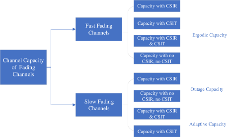
Figure 19: An overview of performance metrics for fading channels.

Considering wireless fading time-varying channels, we can distinguish fast fading and slow fading and further classify each case into subcases each with or without Channel State Information at Transmitter (CSIT) and/or Channel State Information at Receiver (CSIR), see Fig. 19. Two capacity definitions are reviewed:

• Ergodic capacity: In the case of fast fading, the coding block length spans a large number of channel coherence time intervals. The channel is thus ergodic (i.e., each codeword seeing all possible fading realizations) and has a well-defined Shannon ergodic capacity. For a single-user channel with perfect CSIR and CSIT, the ergodic capacity is given by

  $$C_{CSIR/CSIT} =\underset{p\left(X\mid H\right)}{\max}\mathbb{E}_{H}\left[I\left(X;Y\mid H=h\right)\right]$$ (17)

  $$\text{s.t. }\mathbb{E}\left[\left|X\right|^{2}\right]\leq P,$$

  which is attained by adapting the transmission power and rate to the channel state variations, i.e., the input distribution $p\left(X\mid H\right)$ depends on the channel state $H$. On the other hand, if with perfect CSIR but without CSIT, no adaptive transmission strategy is allowed and the ergodic capacity reduces to

  $$C_{CSIR} =\underset{p\left(X\right)}{\max}\text{ }\mathbb{E}_{H}\left[I\left(X;Y\mid H=h\right)\right]$$ (18)

  $$\text{s.t. }\mathbb{E}\left[\left|X\right|^{2}\right]\leq P.$$ (19)

  In this case, the input distribution $p\left(X\right)$ does not depend on the channel state $H$ anymore.

• Outage capacity: In the case of slow fading, the coding block length is on the order of the channel coherence time interval. The channel is thus no longer ergodic and Shannon capacity is not well defined in this case. However, if the system can tolerate a loss of a fraction $p_{out}$ of the messages on average, reliable communication can be achieved at any rate lower than an outage capacity. For a single-user channel with perfect CSIR without CSIT, the outage capacity is given by

  $$C_{out} =\underset{\begin{array}[]{c}p\left(X\right):\mathbb{E}\left[\left|X\right|^{2}\right]\leq P\end{array}}{\max}R$$ (21)

  $$\text{ s.t. }p\left(I\left(X;Y\mid H=h\right)<R\right)\leq p_{out}.$$ (22)

The definitions above can also be generalized to the multiuser scenario, leading to ergodic capacity region and outage capacity region, see, e.g., [67], [68]. More information-theoretic modeling and fundamental limits on the state-dependent channels can also be found in [69].

III-B3 Summary

Shannon capacity serves as an ultimate limit that a communication system can achieve. In addition to its theoretical importance, the establishment of the capacity can also guide the design of capacity-achieving structured codes (such as LDPC and polar codes) and drive innovative transmission strategy, such as adaptive power and rate transmission in the ergodic fading case. However, Shannon capacity is not always well defined in particular when the channel is time-varying and the transmitter or receiver may or may not access to all realizations or the full statistics of the channel state. Alternative approaches, such as outage capacity here, or adaptive capacity and broadcast capacity [67], [68] can be useful in characterizing the performance bounds of such a communication system.

III-C Performance Metrics for ISAC

In the above two subsections, we have presented some performance metrics for sensing and communication functionalities, respectively. ISAC systems aim to integrate both functionalities in a synergetic manner and therefore fundamental communication-sensing performance tradeoff should be fully understood. Towards this end, a unified capacity-distortion performance metric is considered, where the capacity measures the communication performance as presented in Subsection III-B, while the distortion notion slightly generalizes the MSE as in Subsection III-A to account for estimation of parameters of finite alphabet and to accommodate arbitrary estimation cost function. In the following, we review three approaches for representing the capacity-distortion tradeoff in the literature. We would like to point out that the existing performance metrics for ISAC are still primeval and thus deserve further study.

III-C1 Estimation-Information-Rate Induced Approach

The estimation information rate was introduced by [70] and represents an approximate mutual information between the observation $Y$ and the true parameter $\theta$. Specifically, consider $\theta$ is Gaussian distributed with variance $P$ and it is estimated as $\hat{\theta}$ with MSE distortion $D$. It is standard to establish the following inequality chain

$$I\left(\theta;Y\right)\geq I\left(\theta;\hat{\theta}\right)\geq\frac{1}{2}\log\left(\frac{P}{D}\right),$$ (23)

where the first inequality uses the Markov chain $\theta-Y-\hat{\theta}$ and follows by the data processing inequality, while the second inequality holds because

$$\begin{array}[]{l}I\left(\theta;\hat{\theta}\right)=h\left(\theta\right)-h\left(\theta\mid\hat{\theta}\right)\\ \geq h\left(\theta\right)-h\left(\theta-\hat{\theta}\right)\\ \geq h\left(\theta\right)-\frac{1}{2}\log\left(2\pi e\mathbb{E}\left[\left(\theta-\hat{\theta}\right)^{2}\right]\right).\end{array}$$ (24)

This lower bound therefore converts the MSE distortion to an estimation information rate for sensing. Hence one can examine the tradeoff between the communication information rate and the estimation information rate both in the same unit for ISAC systems.

III-C2 Equivalent-MSE Induced Approach

Instead of deriving equivalent estimation information rate for sensing, [71] proposed to derive the equivalent of communication information rate to the MSE metric. In particular, consider a Gaussian channel $Y=\sqrt{snr}X+Z$, where $X,Z\sim\mathcal{CN}\left(0,1\right)$. Then the MMSE of estimating input $X$ from output $Y$ is given by: $D\left(snr\right)=1/\left(1+snr\right)$. Therefore one can convert a given communication capacity $C\left(snr\right)=\log\left(1+snr\right)$ to a MSE metric by $D_{\textrm{Equivalent}}=2^{-C}$ . In this way, one can examine the tradeoff between the communication equivalent-MSE and the estimation MSE both in the same unit for ISAC systems.

III-C3 Capacity-Distortion Function Induced Approach

Different from traditional channel capacity, the capacity-distortion function $C\left(D\right)$ is the channel capacity under certain distortion constraints $D$ since we need to send message while simultaneously estimating the channel state $S$ [72],[20]. Specifically, a general capacity-distortion function is given by

$$C\left(D\right)=\underset{p\left(X\right)}{\max}\text{ }I\left(X;Y\mid S\right),\text{ s.t. }\mathbb{E}\left[d\left(S,\hat{S}\right)\right]\leq D,$$ (25)

where $X,Y$ are input and output symbol respectively, $\hat{S}$ is the estimated sensing state and $\mathbb{E}\left[d\left(S,\hat{S}\right)\right]$ is the average distortion of an estimator. More details can be found in Section VI and Section VII.

III-C4 Summary

The first two approaches above represent very preliminary attempts at constructing a unified capacity-distortion performance metric for ISAC systems. Each has its own obvious limitations. The first approach assumes Gaussian distributed sensing parameters and estimation errors and requires to know the MSE of an estimator, while the second approach also works only in a simple linear Gaussian channel modeling. The third approach seems to be a more natural way to unify the analysis of the fundamental limits of ISAC under the information-theoretic framework. However, the current information-theoretic models considered in [72],[20] are oversimple and cannot cover many important ISAC scenarios. As such, new frameworks and more general approaches are called upon for better characterizing the performance limits of ISAC.

IV Fundamental Limits of Device-free Sensing

In this section, we will discuss the current research progress on the fundamental limits of device-free sensing. In particular, we will focus on the fundamental limits for different classes of radar sensing as classified in Section II. For each class, we will highlight several important works, and present the system model, performance bounds and key insights learned from the analysis of the fundamental limits.

IV-A Fundamental Limits of Phased-array Radar

A few works have investigated the fundamental limits of phased-array radar. In [65], the author studied the performance limits of the mono-static phased-array radar system with a single transmit antenna and $N$ receive antennas. Assuming that the target is quasi-static and the Doppler effect can be ignored, the $N$-dimensional received signal for one radar pulse is given by

$$\boldsymbol{Y}(t)=\alpha\boldsymbol{a}_{R}(\theta)s\left(t-\tau\right)+\boldsymbol{Z}(t),$$ (26)

where $\alpha$ is the reflection coefficient of the target, $\tau$ is the delay of the target, $\boldsymbol{a}_{R}(\theta)=[e^{j\frac{2\pi}{\lambda}R_{1}\sin\theta},e^{j\frac{2\pi}{\lambda}R_{2}\sin\theta},\cdots,e^{j\frac{2\pi}{\lambda}R_{N}\sin\theta}]^{T}$ is the receive steering vector with $R_{n}$ denoting the locations of the $n$-th antennas, $s\left(t\right)$ is the transmit waveform with normalized energy and $\boldsymbol{Z}(t)$ is the noise matrix, including the interfering echoes from the clutters and the background noise. The noise matrix has i.i.d complex Gaussian entries of zero mean and variance $\sigma_{z}^{2}$. Under these assumptions, the CRBs of delay $\tau$ and direction of arrival (DOA) $\theta$ are given by

$$CRB_{\tau}=\frac{1}{8\pi^{2}\textrm{SNR}N\beta^{2}},$$ (27)

$$CRB_{\theta}=\frac{6}{\left(2\pi\right)^{2}\frac{d^{2}}{\lambda^{2}}\cos^{2}\theta\textrm{SNR }N\left(N^{2}-1\right)},$$ (28)

where $\beta^{2}=\frac{\int_{-\infty}^{\infty}f^{2}\left|S(f)\right|^{2}df-\left(\int_{-\infty}^{\infty}f\left|S\left(f\right)\right|^{2}df\right)^{2}}{\int_{-\infty}^{\infty}\left|S(f)\right|^{2}df}$ is the squared effective bandwidth, $S(f)$ is the Fourier transformation of transmitted baseband signal $s(t)$, $\text{SNR}=\frac{\left|\alpha\right|^{2}}{\sigma_{z}^{2}}$ is the received SNR, $\lambda$ is the signal wavelength, and $d$ is antenna spacing. Note that if $\left|S\left(f\right)\right|$ is symmetric with respect to zero, the right integral representation $\int_{-\infty}^{\infty}f\left|S\left(f\right)\right|^{2}df$ will become zero.

From (27) and (28), we conclude that the estimation performance of both delay $\tau$ and DOA $\theta$ improves with the increase of SNR and the number of receive antennas $N$. In addition, the estimation performance of $\tau$ also improves with the increase of the squared effective bandwidth $\beta^{2}$, while the estimation performance of $\theta$ improves with the increase of the normalized antenna spacing $d/\lambda$.

The performance limits of the mono-static phased-array radar system with multi-antenna transmit and receive arrays was further studied in [73], in terms of CRB. The system model is illustrated in Fig. 20. Uniform linear array (ULA) is adopted as the transmit/receive array and the spacing $d$ between two adjacent antennas is assumed to be half of the signal wavelength $\lambda$. Both transmit and receive antenna arrays are assumed to have $M$ antennas. Additionally, the target is assumed to be static (i.e., there is no Doppler shift). In this case, the target parameters are range $r$ and DOA $\theta$. The range $r$ is estimated from the time delay $\tau$ according to the relationship $r=\tau c/2$, while the DOA $\theta$ is estimated directly based on the received radar echo. Specifically, the $M\times 1$ received signal for one radar pulse is given by

$$\boldsymbol{Y}(t)=\alpha\boldsymbol{a}_{R}(\theta)\boldsymbol{a}_{T}^{T}(\theta)\boldsymbol{w}s\left(t-\tau\right)+\boldsymbol{Z}(t),$$ (29)

where $\alpha$ is the reflection coefficient of the target, $\boldsymbol{a}_{T}(\theta)$ is the transmit steering vector, and $\boldsymbol{w}=\left[w_{1},\ldots,w_{M}\right]^{T}$ is the beamforming vector. To facilitate the analysis, the beamforming vector is assumed to be $\boldsymbol{w}=\boldsymbol{a}_{T}(\theta)$ in [73] to obtain the highest possible processing gain at the actual DOA $\theta$.

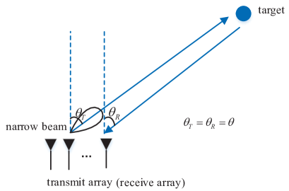
Figure 20: Single-target sensing in the mono-static phased-array radar system.

Under the above assumptions, the CRB of $r$ and $\theta$ is given by [73]

$$CRB_{r} =\frac{3}{2\pi^{2}\text{SNR}M^{3}\beta^{2}},$$ (30)

$$CRB_{\theta} =\frac{1}{2\text{SNR}M^{3}\xi^{2}},$$ (31)

where $\beta^{2}$ is the squared effective bandwidth and

$$\xi^{2}=\frac{\pi^{2}d^{2}\cos^{2}\theta(M^{2}-1)}{3\lambda^{2}}$$ (32)

is the root mean square aperture width of the beampattern.

From (31) and (30), we can make similar conclusion as that for the case of single transmit antenna. The main difference is that the CRB in (31) for the case of $M$ transmit antennas has an additional factor of $1/M^{2}$, which is contributed by the transmit beamforming gain and that the total transmit power increases with the number of transmit antennas $M$ when the transmit power of each transmit antenna is fixed.

IV-B Fundamental Limits of MIMO Radar

IV-B1 Colocated MIMO Radar for Single-Target Sensing

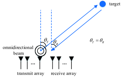
Figure 21: Single-target sensing via colocated MIMO radar.

The CRB of the sensing performance via colocated MIMO radar has been studied in [36] for single-target sensing. The system model is illustrated in Fig. 21. In the system model, a colocated MIMO radar formed by $M$ transmit antennas and $N$ receive antennas is used to detect a moving target. The MIMO radar is assumed to be moving with the velocity $v_{S}$ and $L$ radar pulses are transmitted in a coherent processing interval (CPI) for target sensing. At the radar receiver, a matched filter bank is used to estimate the time delay first, and then the signals after the matched filter bank are assumed to be sampled at the perfect timing without any delay estimation error. Finally, the discrete samples after matched filtering are used to estimate the DoA $\theta$ and velocity $v$ of the target. Specifically, after the matched filter bank, the $N\times M$ received signal for the $l$-th radar pulse is given by

$$\boldsymbol{Y}(l)=\alpha\boldsymbol{a}_{R}(\theta)\boldsymbol{a}_{T}^{T}(\theta)e^{j2\pi f_{D}l}+\boldsymbol{Z}(l),$$ (33)

where $\alpha$ is the reflection coefficient of the target, $\boldsymbol{a}_{T}(\theta)=[e^{j\frac{2\pi}{\lambda}T_{1}\sin\theta},e^{j\frac{2\pi}{\lambda}T_{2}\sin\theta},\cdots,e^{j\frac{2\pi}{\lambda}T_{M}\sin\theta}]^{T}$ is the transmit steering vector and $\boldsymbol{a}_{R}(\theta)=[e^{j\frac{2\pi}{\lambda}R_{1}\sin\theta},e^{j\frac{2\pi}{\lambda}R_{2}\sin\theta},\cdots,e^{j\frac{2\pi}{\lambda}R_{N}\sin\theta}]^{T}$ is the receive steering vector, $T_{m}$ and $R_{n}$ are the locations of the $m$-th and $n$-th sensors for the transmit and receive antennas respectively, $f_{D}=2T_{P}(v_{S}sin(\theta)+v)/\lambda$ is the normalized Doppler frequency and $T_{P}$ is the radar pulse period, and $\boldsymbol{Z}(l)$ is the noise matrix with i.i.d complex Gaussian entries of zero mean and variance $\sigma_{z}^{2}$.

Assuming that the linear array is used, the CRBs of $\theta$ and $v$ are given by [36]

$$CRB_{\theta}=\frac{1}{2\text{SNR}\pi^{2}\cos^{2}\theta MNL(\sigma_{R}^{2}+\sigma_{T}^{2})},$$ (34)

$$CRB_{v}=\frac{1}{8\text{SNR}\pi^{2}MNL}\left(\frac{3\lambda^{2}}{(L^{2}-1)T_{P}^{2}}+\frac{4v_{S}^{2}}{\sigma_{R}^{2}+\sigma_{T}^{2}}\right),$$ (35)

where $\text{SNR}=\frac{\left|\alpha\right|^{2}}{\sigma_{z}^{2}}$ is the received SNR, $L$ is the number of radar pulses in a CPI, $\sigma_{T}^{2}$ and $\sigma_{R}^{2}$ are the sample-variances of the transmit and receive antenna positions, which are defined as

$$\sigma_{R}^{2} =\frac{4}{N\lambda^{2}}\left(\tilde{\kappa_{R}}-\frac{\kappa_{R}^{2}}{N}\right),$$

$$\sigma_{T}^{2} =\frac{4}{M\lambda^{2}}\left(\tilde{\kappa_{T}}-\frac{\kappa_{T}^{2}}{M}\right),$$

where $\tilde{\kappa_{R}}=\sum_{n=0}^{N-1}R_{n}^{2}$, $\tilde{\kappa_{T}}=\sum_{m=0}^{M-1}T_{m}^{2}$, $\kappa_{R}=\sum_{n=0}^{N-1}R_{n}$ and $\kappa_{T}=\sum_{m=0}^{M-1}T_{m}$.

Note that the sample-variances of the transmit and receive antenna positions $\sigma_{R}^{2}$ and $\sigma_{T}^{2}$ are related to the root mean square aperture width of the beampattern $\xi^{2}$ in (32). Specifically, if both the transmit and receive antenna arrays are uniform linear arrays (ULAs) with $M$ antennas and antenna spacing $d$, we have

$$\pi^{2}\cos^{2}\theta(\sigma_{R}^{2}+\sigma_{T}^{2})=O\left(\frac{\pi^{2}d^{2}\cos^{2}\theta M^{2}}{\lambda^{2}}\right),$$

which has the same order as $\xi^{2}$. In this case, if $L=1$, the order of the CRB of $\theta$ in (34) is given by

$$CRB_{\theta}=O\left(\frac{1}{\text{SNR}M^{2}\xi^{2}}\right).$$

Compared to the order of the CRB of $\theta$ for the phased-array radar in (31), i.e., $O\left(\frac{1}{\text{SNR}M^{3}\xi^{2}}\right)$, the CRB of $\theta$ for the colocated MIMO radar decreases with $M$ at the order of $1/M^{2}$ instead of $1/M^{3}$. This is not surprising since the phased-array radar can focus its transmit energy on the direction of the target to achieve a beamforming gain of $O\left(M\right)$, while the colocated MIMO radar cannot enjoy such beamforming gain since it transmits independent waveforms from different antennas. However, the advantage of MIMO radar is that its transmit signal can cover the whole angular space and thus the initial search time for a target can be reduced.

From (34) and (35), it can be observed that the the estimation performance of the DOA $\theta$ and velocity $v$ is positively relative to SNR, the number of pulses $L$ in a CPI, the product of the transmit and receive antennas $MN$ and the sample-variances of the antenna positions $\sigma_{R}^{2},\sigma_{T}^{2}$. The estimation performance of the velocity also improves with the increase of the radar pulse period $T_{P}$ and the decrease of the radar velocity $v_{S}$ and signal wavelength $\lambda$. However, the movement of the radar has no impact on the estimation performance of the DOA of the target.

In [37], the CRB of colocated MIMO radar using time multiplexing is analysed. The obtained CRB shows that the accuracy of the DOA estimators decreases in a MIMO radar if the target moves with relative radial velocity, because the motion causes an unknown phase rotation of the baseband signal due to the Doppler effect.

IV-B2 Colocated MIMO Radar for Multi-Target Sensing

Figure 22: Multi-target sensing via colocated MIMO radar.

In [74], the CRB analysis of the colocated MIMO radar is extended to the multi-target case, as illustrated in Fig. 22. There are $K$ targets and the DOA of the $k$-th target is $\theta^{k}$. The transmit signal is narrowband and thus the time delay is ignored in the system model. After the matched filter bank, the $N\times M$ received signal for the $l$-th radar pulse is given by

$$\boldsymbol{Y}(l)=\sum_{k=1}^{K}\alpha^{k}\boldsymbol{a}_{R}(\theta^{k})\boldsymbol{a}_{T}^{T}(\theta^{k})e^{j2\pi f_{D}^{k}l}+\boldsymbol{Z}(l),$$ (36)

where $\alpha^{k}$ is the reflection coefficient of the $k$-th target, $\boldsymbol{a}_{T}(\theta^{k})$ and $\boldsymbol{a}_{R}(\theta^{k})$ are the transmit and receive steering vectors respectively, $f_{D}^{k}$ is the Doppler shift associated with the $k$-th target, and $\boldsymbol{Z}(l)$ is the noise matrix.

The target parameters are the DOAs $\theta^{k}$’s and velocities $v^{k}$’s of the targets, where the velocity $v^{k}$ is estimated from the Doppler shift $f_{D}^{k}$. In [74], the special case of two targets is studied in details. To facilitate analysis, intermediate target parameters $\vartheta^{1}$, $\vartheta^{2}$, $f_{D}^{1}$ and $f_{D}^{2}$ are adopted, where $\vartheta^{1}=sin(\theta^{1})$ and $\vartheta^{2}=sin(\theta^{2})$. CRB of these intermediate parameters is deduced. Since the expression of the CRB is very complicated, we do not give the exact expression. The main conclusion is that the CRB of the DOAs and velocities of the two targets only depends on the differences of their DOAs and Doppler frequencies, i.e.,

$$CRB_{\vartheta^{1},\vartheta^{2},f_{D}^{1},f_{D}^{2}}=CRB_{\vartheta^{1},\vartheta^{2},f_{D}^{1},f_{D}^{2}}(\bigtriangleup\vartheta,\bigtriangleup f_{D})$$ (37)

where $\bigtriangleup\vartheta=\vartheta^{1}-\vartheta^{2}$ and $\bigtriangleup f_{D}=f_{D}^{1}-f_{D}^{2}$. The estimation performance is better if the differences $\bigtriangleup\vartheta,\bigtriangleup f_{D}$ between the parameters of the two targets are larger. When $\bigtriangleup\vartheta$ and $\bigtriangleup f_{D}$ are sufficiently large, the estimation performance for two targets will approach that for a single target.

IV-B3 Distributed MIMO Radar for Single-Target Sensing

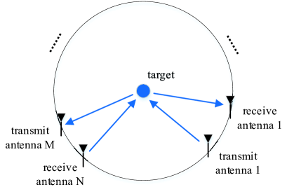
Figure 23: Single-target sensing via distributed MIMO radar.

The CRB of the sensing performance via the distributed MIMO radar has been studied in [39] for single-target sensing. As illustrated in Fig. 23, the transmit and receive antennas are placed symmetrically around the target so that the sensing performance can be improved [39]. The lowpass equivalent of the signal transmitted from the $m$-th transmitter is $s_{m}(t)$, and the energy of the waveform $s_{m}(t)$ is normalized to be one. Assume that the transmitted signals $s_{m}(t)$’s from different transmit antennas are approximately orthogonal and they maintain approximate orthogonality for time delays and Doppler shifts of interest. Under these assumptions, the received signal model at receiver $n$ due to the signal transmitted from transmitter $m$ is

$$y_{n,m}(t)=\alpha_{n,m}s_{m}(t-\tau_{n,m})e^{j2\pi f_{n,m}t}+z_{n,m}(t),$$ (38)

where $\tau_{n,m}$, $f_{n,m}$ and $\alpha_{n,m}$ represent the time delay, Doppler shift and reflection coefficients, respectively, corresponding to the path between the $m$-th transmitter and the $n$-th receiver, and $z_{n,m}(t)$ is noise.

The parameters of interest are the location and velocity of the target, which are expressed in the form of coordinates in rectangular coordinate systems as $(x,y)$ and $(v_{x},v_{y})$. These parameters are estimated from the time delays $\tau_{n,m}$ and Doppler shifts $f_{n,m},1\leq n\leq N,1\leq m\leq M$, which can be regarded as intermediate parameters.

Since the number of the intermediate parameters is large, it is difficult to obtain a closed-form expression of CRB. Nonetheless, we can analyse the order of the CRB for the time delay and Doppler shift of the path between transmitter $m$ and receiver $n$, as given by

$$CRB_{\tau_{n,m}}=O\left(\frac{1}{\textrm{SNR}_{n,m}\beta_{m}^{2}}\right),$$ (39)

$$CRB_{f_{n,m}}=O\left(\frac{1}{\textrm{SNR}_{n,m}\gamma_{n,m}^{2}}\right),$$ (40)

where $\beta_{m}^{2}$ is the squared effective bandwidth of $s_{m}(t)$, $\textrm{SNR}_{n,m}=\frac{\left|\alpha_{n,m}\right|^{2}}{\sigma_{z}^{2}}$ and

$$\gamma_{n,m}^{2}$$

$$= \frac{\int_{-\infty}^{\infty}t^{2}\left|s_{m}(t-\tau_{n,m})\right|^{2}dt-\left|\int_{-\infty}^{\infty}t\left|s_{m}(t-\tau_{n,m})\right|^{2}dt\right|^{2}}{\int_{-\infty}^{\infty}\left|s_{m}\left(t\right)\right|^{2}dt},$$

are the received SNR and squared effective pulse length for the $(n,m)$-th receive-transmit pair, respectively. Furthermore, assume that $\textrm{SNR}_{n,m}=O\left(\text{SNR}\right),\gamma_{n,m}^{2}=O\left(\gamma^{2}\right),\forall n,m$ and $\beta_{m}^{2}=O\left(\beta^{2}\right),\forall m$, where $\text{SNR}=\frac{1}{NM}\stackrel{{\scriptstyle[}}{{n}}=1]{N}{\sum}\stackrel{{\scriptstyle[}}{{m}}=1]{M}{\sum}\textrm{SNR}_{n,m},$ $\gamma^{2}=\frac{1}{NM}\stackrel{{\scriptstyle[}}{{n}}=1]{N}{\sum}\stackrel{{\scriptstyle[}}{{m}}=1]{M}{\sum}\gamma_{n,m}^{2}$ and $\beta^{2}=\frac{1}{M}\stackrel{{\scriptstyle[}}{{m}}=1]{M}{\sum}\beta_{m}^{2}$ are the average received SNR, average squared effective pulse length and average squared effective bandwidth, respectively. Then it can be shown that the orders of the CRB for the position and velocity are respectively given by [39]

$$CRB_{(x,y)}=O\left(\frac{1}{\textrm{SNR}MN\left(\beta^{2}+\gamma^{2}\right)}\right),$$ (41)

$$CRB_{(v_{x},v_{y})}=O\left(\frac{1}{\textrm{SNR}MN\gamma^{2}}\right).$$ (42)

The key insights revealed from the CRB analysis in [39] is that the estimation performance improves with the number of antennas $M,N$ and SNR. Moreover, the estimation performance of the position $(x,y)$ improves with both the squared effective bandwidth and squared effective pulse length, while the estimation performance of the velocity $(v_{x},v_{y})$ improves with the squared effective pulse length.

In [40], the CRB is also analyzed for directly estimating the velocity of the target only. It is concluded that the estimation performance of the velocity is also positively relative to the SNR and the squared effective radar pulse length.

IV-B4 Distributed MIMO Radar for Multi-Target Sensing

In [41], the CRB analysis of the distributed MIMO radar is extended to the multi-target case. Under similar assumptions as in [39], the received signal model at receiver $n$ due to the signal transmitted from transmitter $m$ and the reflection of all the $K$ targets is

$$y_{n,m}(t)=\sum_{k=1}^{K}\alpha_{n,m}^{k}s_{m}(t-\tau_{n,m}^{k})e^{j2\pi f_{n,m}^{k}t}+z_{n,m}(t),$$ (43)

where $\tau_{n,m}^{k}$, $f_{n,m}^{k}$ and $\alpha_{n,m}^{k}$ represent the time delay, Doppler shift and reflection coefficients, respectively, corresponding to the path from the $m$-th transmitter to the $k$-th target and then reflected to the $n$-th receiver.

The target parameters are the locations and velocities of the targets, which are expressed in the form of coordinates in rectangular coordinate systems as $(x^{k},y^{k})$ and $(v_{x}^{k},v_{y}^{k}),1\leq k\leq K$. These parameters are estimated from time delay $\tau_{m,n}^{k}$ and Doppler shifts $f_{m,n}^{k},1\leq m\leq M,1\leq n\leq N,1\leq k\leq K$ , which can be regarded as intermediate parameters.

The key insights revealed from the CRB analysis in [41] is that if the distances between the targets are large enough, the interactions between the multiple targets can be ignored and the performance of the multiple-target sensing can approach that of the single-target sensing.

IV-C Fundamental Limits of Phased-MIMO Radar

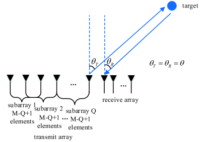
Figure 24: Single-target sensing via phased-MIMO radar.

The existing works have been focusing on investigating the performance limits of single-target sensing in the mono-static phased-MIMO radar system. In [32], ambiguity function (AF) is adopted to analyse the performance of phased-MIMO radar. The system model is illustrated in Fig. 24. In phased-MIMO radar, the transmit array is divided into $Q$ subarrays, while each subarray contains $P=M-Q+1$ adjacent antennas. Meanwhile, the spacings between two adjacent antennas of the transmit and receive arrays are assumed to be $d_{T}$ and $d_{R}$, respectively. Additionally, the reflection coefficient is assumed to be 1 and noise is ignored to simplify the analysis of AF. Under these assumptions, the $N\times 1$ received signal is given by

$$\boldsymbol{y}(t,\tau,f_{D},\theta) =\boldsymbol{a}_{R}(\theta)\sum_{q=1}^{Q}\boldsymbol{a}_{q}^{T}(\theta)\boldsymbol{w}_{q}e^{-j2\pi f_{c}\tau_{q}\text{($\theta$)}}$$ (44)

$$\times s_{q}(t-\tau)e^{j2\pi f_{D}t}e^{-j2\pi(f_{c}+f_{D})\tau},$$ (45)

where $\tau$ is the round-trip delay for a target in the $\theta$ direction, $f_{D}$ is the Doppler shift, $f_{c}$ is the carrier frequency, $\tau_{q}\text{($\theta$)}=qd_{T}\sin\theta/c$ is the relative delay of the zeroth element of the $q$-th subarray with respect to the zeroth element of the zeroth subarray, $\boldsymbol{a}_{R}(\theta)$ is the receive steering vector, $\boldsymbol{a}_{q}(\theta)$, $s_{q}(t)$ and $\boldsymbol{w}_{q}$ are the transmit steering vector, transmit waveform and transmit beamforming vector for the $q$-th subarray, respectively. Note that we have explicitly express the received signal as a function of $\tau,f_{D},\theta$.

$$\intop_{-\infty}^{\infty}\boldsymbol{y}^{H}(t,\tau^{\prime},f_{D}^{\prime},\theta^{\prime})\boldsymbol{y}(t,\tau,f_{D},\theta)dt=\boldsymbol{a}_{\boldsymbol{R}}^{H}(\theta^{\prime})\boldsymbol{a}_{\boldsymbol{R}}(\theta)\intop_{-\infty}^{\infty}\sum_{q=1}^{Q}(\boldsymbol{w}_{q}^{H}\boldsymbol{a}_{q}^{*}(\theta)s_{q}(t-\tau^{\prime}))\sum_{q=1}^{Q}(\boldsymbol{a}_{q}^{T}(\theta)\boldsymbol{w}_{q}s_{q}(t-\tau))e^{j2\pi(f_{D}-f_{D}^{\prime})t}dt.$$ (46)

TABLE II: Comparison of different classes of radars.

Types of Radar	Phased-array Radar	Distributed MIMO Radar	Colocated MIMO Radar
CRB order for $\tau$	$O\left(\frac{1}{\text{SNR}NM^{2}L\beta^{2}}\right)$	$O\left(\frac{1}{\text{SNR}\beta^{2}L}\right)$	$O\left(\frac{1}{\text{SNR}NM\beta^{2}L}\right)$
CRB order for $\theta$	$O\left(\frac{1}{\text{SNR}NM^{2}L\cos^{2}\left(\theta\right)\left(\sigma_{R}^{2}+\sigma_{T}^{2}\right)}\right)$	N/A	$O\left(\frac{1}{\text{SNR}NML\cos^{2}\left(\theta\right)\left(\sigma_{R}^{2}+\sigma_{T}^{2}\right)}\right)$
CRB order for $f_{D}$	$O\left(\frac{1}{\textrm{SNR}NM^{2}L\gamma^{2}}\right),$	$O\left(\frac{1}{\textrm{SNR}L\gamma^{2}}\right)$	$O\left(\frac{1}{\textrm{SNR}NML\gamma^{2}}\right)$
Advantages	Beamforming Gain	Spatial Diversity Gain	Waveform Diversity Gain
Disadvantages	Long scanning time	High synchronization requirements	SNR degradation

If the matched filters at the receivers are matched to the received signal with a different set of parameters $\tau^{\prime},f_{D}^{\prime},\theta^{\prime}$, then the output of the matched filters combined together can be expressed as in (46) on the top of the next page. The first term on the right-hand side of (46), i.e., $\boldsymbol{a}_{\boldsymbol{R}}^{H}(\theta^{\prime})\boldsymbol{a}_{\boldsymbol{R}}(\theta)$, represents the spatial processing in the receiver and is independent of the transmit waveforms $s_{q}(t),1\leq q\leq Q$. The second term on the right-hand side of (46) is defined as the AF [32], which shows the sensitivity of the output of the matched filter to the error of the estimation of the parameters. The maximum of the AF is achieved when $\tau^{\prime}=\tau$, $f_{D}^{\prime}=f_{D}$ and $\theta^{\prime}=\theta$. The narrower the curve of the AF is, the better the estimator is expected to be.

In contrast to MIMO radar systems in which the ambiguity function is fixed, we can adapt the ambiguity function by changing the size of subarrays and the number of subarrays in the case of phased-MIMO radar [32]. Meanwhile, adopting the linear frequency modulation (LFM) waveform can improve the delay resolution but it is accompanied by the penalty of delay–Doppler coupling [32].

IV-D Summary and Insights

In existing works, CRB and AF have been used as the performance metrics for device-free sensing, among which CRB is the most widely used performance metric. The target parameters to be estimated usually include the time delay $\tau$, the DOA $\theta$ and the Doppler frequency $f_{D}$. The other target parameters such as its location and velocity can be inferred from these intermediate parameters. For all classes of radars, the estimation performance of all target parameters improves with the increase of SNR (power resource), the number of antennas (spatial resource) and the number of pulses in a CPI (time resource), since the increase of these system resources increases the effective SNR and the number of observations for parameter estimation.

Specifically, the order of the CRB for the estimation of the time delay $\tau$ can be expressed in a unified expression as

$$CRB_{\tau}=O\left(\frac{1}{\text{SNR}NM^{a}L\beta^{2}}\right),$$ (47)

where $M$ and $N$ are the number of transmit and receive antennas respectively, $L$ is the number of pulses in a CPI, $\beta^{2}$ is the squared effective bandwidth and the exponent $a$ depends on the type of radar. For example, $a=1$ for MIMO radar and $a=2$ for phased-array radar due to the additional transmit beamforming gain. Clearly, the estimation performance of the time delay $\tau$ also improves with the squared effective bandwidth $\beta^{2}$.

The order of the CRB for the estimation of the DOA $\theta$ for colocated antennas can be expressed in a unified expression as

$$CRB_{\theta}=O\left(\frac{1}{\text{SNR}NM^{a}L\cos^{2}\left(\theta\right)\left(\sigma_{R}^{2}+\sigma_{T}^{2}\right)}\right),$$ (48)

where $\sigma_{T}^{2}$ and $\sigma_{R}^{2}$ are the sample-variances of the transmit and receive antenna positions and $a$ depends on the type of radar. For example, $a=1$ for MIMO radar and $a=2$ for phased-array radar. Clearly, the estimation performance of the DOA $\theta$ also improves with the sample-variances of the transmit and receive antenna positions $\sigma_{T}^{2}$ and $\sigma_{R}^{2}$.

The order of the CRB for the estimation of the Doppler frequency $f_{D}$ can be expressed in a unified expression as

$$CRB_{f_{D}}=O\left(\frac{1}{\textrm{SNR}NM^{a}L\gamma^{2}}\right),$$ (49)

where $\gamma^{2}$ is the squared effective pulse length and $a$ depends on the type of radar. For example, $a=1$ for MIMO radar and $a=2$ for phased-array radar. Clearly, the estimation performance of the Doppler frequency $f_{D}$ also improves with the squared effective pulse length $\gamma^{2}$.

From the above unified expressions, we can conclude that the SNR, the number of transmit (receive) antennas $M$ ($N$), and the number of pulses in a CPI are the common influence factors on the estimation of time delay $\tau$, the DOA $\theta$ and the Doppler frequency $f_{D}$, while the estimation of $\tau$, $\theta$ and $f_{D}$ are also determined by $\beta$ (effective bandwidth), $\sigma_{R}^{2}$ and $\sigma_{T}^{2}$ (antenna geometry), and $\gamma$ (effective pulse length), respectively. To summarize, the comparison of order-wise performances of different classes of radars and their pros and cons are listed in Table II. There are two additional comments to the CRB order in Table II. First, for the distributed MIMO radar, the order of the CRB is given for the intermediate parameters associated with the path between one transmit and receive antenna pair. However, the final estimation for the position and velocity of the target is obtained from the estimates of intermediate parameters of the paths between all transmit and receive antenna pairs. It can be shown that the estimation performance of the position and velocity in the distributed MIMO radar actually has the same order as that in the colocated MIMO radar [36]. Second, in Table II, we follow the convention in the literature on the fundamental limits of radar sensing and assume a per-antenna power constraint where the transmit power of each antenna is fixed. In this case, the total transmit power increases with the number of transmit antennas $M$. If a total power constraint is assumed, the CRB order for the phased-array radar and colocated MIMO radar should be multiplied by a factor of $M$.

For multi-target MIMO radar, the CRB can be improved if the distances between the targets are larger. In particular, if the targets are sufficiently far away from each other, the parameters of different targets can be estimated independently and the performance of the multiple-target sensing can approach that of the single-target sensing.

V Fundamental Limits of Device-based Sensing

In this section, we will discuss the current research progress on the fundamental limits of device-based sensing. In particular, we will focus on the fundamental limits for different classes of wireless-based localization as classified in Section II. For each class, we will highlight several important works, and present the system model, performance bounds and key insights learned from the analysis of the fundamental limits.

V-A Non-cooperative Wireless Localization

V-A1 TOA-based Localization

The TOA-based localization is the most widely studied wireless localization method. In the following, we first give a brief historical review of the key works on the fundamental limits of the TOA-based localization. Then we discuss the signal model of the TOA-based localization, the fundamental limits and the associated key insights. In [75], Qi et al. first derived the CRB of the TOA-based localization in the presence of non-line-of-sight (NLOS) environment where a single path propagation (either a single LOS or NLOS path) is assumed [75]. The authors concluded that NLOS signals do not contribute to the localization performance when no prior NLOS statistics are available. Furthermore, the CRB is inversely proportional to the square of effective bandwidth and depends on geometric configuration of agent/anchor nodes. When prior information of NLOS signals is attained, the NLOS signals can also provide useful information for localization and the localization accuracy can be improved [76]. In [77], the authors further extended their previous work from the single path propagation case to the multi-path propagation case. Later, further analysis was developed by Shen et al. [78] when the prior knowledge of the agent’s position is available in addition to the NLOS statistics. In [78], the concepts of equivalent FIM (EFIM) and squared position error bound (SPEB) were introduced to develop a general framework for the analysis of the fundamental limits of device-based localization. Besides, map information of the environment can be regard as a special form of prior information to the agent, which helps to improve the estimation accuracy by exploiting some features of the map (e.g., its shape and area) [79]. Furthermore, dynamic scenarios with moving agents are also investigated in [80, 81]. In [80], the performance limit is derived in both static and dynamic scenarios. In the dynamic scenario, the Doppler shift contributes additional direction information with intensity determined by the speed of the agent and the root mean squared time duration of the transmitted signal. In [81], Li proposed a posterior CRB (P-CRB) for the fundamental limit analysis with dynamic sensor networks.

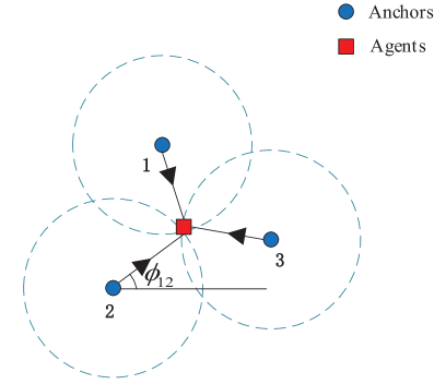
Figure 25: An illustration of TOA-based localization.

To reveal more insights into fundamental limits of the TOA-based localization, we consider a general TOA-based localization scenario studied in [78, 22]. In this case, consider a multi-path environment which commonly exists in wireless network and the wireless network consists of $N_{a}$ agent nodes and $N_{b}$ anchor nodes in a 2-D plane, as illustrated in Fig. 25. We define $\mathcal{N}_{a}=\left\{1,...,N_{a}\right\},\mathcal{N}_{b}=\left\{1,...,N_{b}\right\}$ as the set of agent nodes and anchor nodes, respectively. The signal transmitted from anchor $j\in\mathcal{N}_{b}$ and received by agent $k\in\mathcal{N}_{a}$ can be written as

$$y_{k,j}\left(t\right)=\sum_{l=1}^{L_{k,j}}\alpha_{k,j}^{\left(l\right)}s\left(t-\tau_{k,j}^{(l)}\right)+z_{k,j}\left(t\right),$$ (50)

where $L_{k,j}$ is the number of multipath components, $\alpha_{k,j}^{\left(l\right)}$ and $\tau_{k,j}^{(l)}$ are the complex gain and delay of $l$-th path, $s(t)$ is a known waveform whose Fourier transform is denoted by $S(f)$, $z_{k,j}\left(t\right)$ represents the observation noise modeled as additive white Gaussian processes with variance $\sigma_{z}^{2}$. The relationship between the delays and the agent position can be expressed as

$$\tau_{k,j}^{\left(l\right)}=\frac{1}{c}\left[\left\|{\bf p}_{k}-{\bf p}_{j}\right\|+b_{k,j}^{\left(l\right)}\right],$$ (51)

where $c$ is the propagation speed of the signal, ${\bf p}_{k}{\bf\triangleq\left[\mathit{x_{k}\textrm{ }y_{k}}\right]^{\mathrm{T}}}$ is the node position, and the range bias $b_{k,j}^{\left(l\right)}>0$ for NLOS propagation while $b_{k,j}^{\left(l\right)}=0$ for LOS propagation.

Since the estimation of individual agent’s location is independent, the analysis can be focused on one agent briefly, e.g., ${\bf p}_{1}$. Define the range information (RI) from an anchor at direction $\phi$ as $\lambda\mathbf{J}_{\text{r}}(\phi)$, where $\lambda$ is a non-negative number called the range information intensity (RII), and ${\bf J}_{\text{r}}\left(\phi\right)$ is a 2 $\times$ 2 matrix named the ranging direction matrix (RDM) with angle $\phi$, given by

$$\mathbf{J}_{\text{r}}(\phi)\triangleq\left[\begin{array}[]{cc}\cos^{2}\phi&\cos\phi\sin\phi\\ \cos\phi\sin\phi&\sin^{2}\phi\end{array}\right].$$ (52)

When the prior knowledge of the agent position and range biases $b_{k,j}^{\left(l\right)}$’s are unavailable, the EFIM for the agent 1’s position is

$$\mathbf{J}_{\text{e}}\left(\mathbf{p}_{1}\right)=\sum_{j\in\mathcal{N}_{\mathrm{b},\mathrm{LOS}}}\lambda_{1,j}\mathbf{J}_{\text{r}}\left(\phi_{1,j}\right),$$ (53)

where $\phi_{1,j}=\tan^{-1}\frac{y_{1}-y_{j}}{x_{1}-x_{j}}$ is the angle from anchor $j$ to agent 1 , $\lambda_{1,j}=\frac{8\pi^{2}\beta^{2}}{c^{2}}\left(1-\chi_{1,j}\right)\text{SNR}_{1,j}^{(1)}$ is the RII from anchor $j$, $\mathcal{N_{\mathrm{b,LOS}}}$ denotes the set of LOS links in $\mathcal{N}_{b}$, $\chi_{1,j}\in[0,1)$ is called path-overlap coefficient (POC), $\beta$ is the effective bandwidth given by $\beta\triangleq\left(\frac{\int_{-\infty}^{+\infty}f^{2}|S(f)|^{2}df}{\int_{-\infty}^{+\infty}|S(f)|^{2}df}\right)^{1/2}$, and $\text{SNR}_{1,j}^{(1)}$ is the receive SNR of the agent 1.

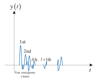
Figure 26: An illustration of the first contiguous cluster (containing paths) in a LOS signal. The first contiguous cluster is defined to be the set of paths $\left\{1,2,...,l\right\}$ such that $\left|\tau_{i}-\tau_{i+1}\right|<T_{s}$ for $i=1,2,...,l-1$, and $\left|\tau_{l}-\tau_{l+1}\right|>T_{s}$ where $T_{s}$ is the duration of $s\left(t\right)$.

The CRB of the position ${\bf p}_{1}$ can be obtained by the matrix inverse $\mathbf{J}_{\text{e}}^{-1}\left(\mathbf{p}_{1}\right)$. Therefore, the EFIM in (53) reveals significant insights into the fundamental limits of wireless network localization. Specifically, the performance of localization relies on the NLOS condition, multipath propagation, network topology and signal bandwidth, as elaborated below.

• When no prior knowledge of range biases is available, NLOS signals make no contribution to the EFIM for the agent position. This is because the relation between delay and the agent position is affected by the unknown range bias as shown in (51).

• The POC $\chi_{1,j}$ characterizes the effect of multipath propagation for localization, which is determined only by the waveform $s(t)$ and the NLOS biases of the multi-path components (MPCs) in the first contiguous cluster [78], as illustrated in Fig. 26. Obviously, the multipath propagation degrades the localization accuracy compared to single-path propagation, since MPCs interfere the estimation of the arrival time of the first path. Moreover, $\chi_{1,j}$ is independent of all the amplitudes. Specially, when the first path is resolvable from the rest paths, $\chi_{1,j}=0$ and the RII reduces to that in the single-path propagation.

• The RII $\lambda_{1,j}$ is proportional to the SNR of the first path in the receiver (agent 1) and the squared effective bandwidth $\beta^{2}$. Moreover, due to the connection with POC $\chi_{1,j}$, larger bandwidth also improves the resolvability of the MPCs.

• The EFIM is the canonical form of a weighted sum of the RDM from individual anchors. Anchor $j$ can provide only 1-D RI at the direction $\varphi_{1,j}$ with intensity $\lambda_{1,j}$ for agent 1. Therefore, the localization performance not only depends on the RII $\lambda_{1,j}$’s but also the ranging direction $\varphi_{1,j}$’s from the anchors. When there are anchors contributing RI from diverse ranging directions $\varphi_{1,j}$’s, the localization performance tends to be better. This phenomenon can be characterized using the notation of information eclipse introduced in [82]. Please refer to [82] for more detailed discussions.

When prior knowledge of the range biases $b_{k,j}^{\left(l\right)}$’s are available, the EFIM for the agent’s position can also be written as a weighted sum of RDMs from individual anchors, given by

$$\tilde{\mathbf{J}}_{\mathrm{e}}\left(\mathbf{p}_{1}\right)=\sum_{j\in\mathcal{N}_{\mathrm{b},\mathrm{LOS}}}\tilde{\lambda}_{1,j}\mathbf{J}_{\mathrm{r}}\left(\phi_{1,j}\right)+\sum_{j\in\mathcal{N}_{\mathrm{b},\mathrm{NLOS}}}\tilde{\lambda}_{1,j}\mathbf{J}_{\mathrm{r}}\left(\phi_{1,j}\right),$$ (54)

where the first and second term on the right-hand side (RHS) indicates the RI of the LOS and NLOS signals, respectively. Moreover, the prior knowledge increases the RII of both LOS and NLOS signals. The RII of NLOS signals can be strictly positive and thus contributes to EFIM in contrast to the case without prior knowledge.

Furthermore, when both prior knowledge of the range biases and the agent’s position is available, the EFIM for the agent’s position is given by

$$\bar{\mathbf{J}}_{\mathrm{e}}\left(\mathbf{p}_{1}\right)=\mathbb{E}_{\mathbf{p}_{1}}\left\{\tilde{\mathbf{J}}_{\mathrm{e}}\left(\mathbf{p}_{1}\right)\right\}+\mathbf{J}_{\mathrm{p}}\left(\mathbf{p}_{1}\right),$$ (55)

where $J_{\mathrm{p}}\left(\mathbf{p}_{1}\right)$ denotes the additional information from the prior position knowledge [78].

V-A2 AOA-based Localization

In the AOA-based localization, the position of the agent is inferred from the AOAs of the LOS paths, which are extracted from the signals from the anchors. The main method of the AOA estimation via antenna arrays is that the differences between the incident signal’s arrival times at different antenna elements contain the angle information. The basic AOA estimation models can be classified into narrowband and wideband models. In the narrowband model, the signal bandwidth $W$ is much less than the center frequency $f_{c}$, and time differences among different antennas can be represented as phase shifts. Hence, phased arrays can be applied to the beam-steering process. In the wideband model, the signal bandwidth $W$ is much larger than the center frequency $f_{c}$. In this case, since a unique phase value cannot represent a time delay for a wideband signal, time delayed lines (timed arrays) are used for the beam-steering, which is the process to form a beam in a specific direction by assigning specific weights at each array antenna elements [83]. Then, some typical scenarios will be discussed in details below.

First, consider the AOA-based localization under narrowband assumption [84], which can be written as

$$\mathbf{y}\left(t\right)=\mathbf{A}\left(\mathbf{\mathbf{\theta}}\right)\mathbf{s}\left(t\right)+\mathbf{z}\left(t\right),$$ (56)

where $t=1,2,\cdots,L$ is the snapshot index, $\mathbf{A}(\theta)=\left[\mathbf{a}\left(\theta_{1}\right),\mathbf{a}\left(\theta_{2}\right),\ldots,\mathbf{a}\left(\theta_{K}\right)\right]\in\mathbb{C}^{N\times K}$ with $\mathbf{a}\left(\theta_{k}\right)$ denoting the steering vector associated with AOA $\theta_{k}$ from the $k$-th source (anchor), $\mathbf{y}\left(t\right)\in\mathbb{C}^{N\times 1}$ is the samples of the received signals, $\mathbf{s}\left(t\right)\in\mathbb{C}^{K\times 1}$ is the source signals, and $\mathbf{z}\left(t\right)\in\mathbb{C}^{N\times 1}$ denotes the additive noise vector with covariance matrix $\sigma_{z}^{2}\boldsymbol{I}$. When $K<N$, the CRB is given by

$$\mathrm{CRB}_{\theta}=\frac{\sigma_{z}^{2}}{2L}\left\{Re\left[\{\mathbf{D}^{H}[\boldsymbol{I}-\mathbf{A}(\mathbf{A}^{H}\mathbf{A})^{-1}\mathbf{A}^{H}]\mathbf{D}\}\right]\right\}^{-1},$$ (57)

where $\mathbf{D}=\left[\frac{d\mathbf{a}\left(\theta_{1}\right)}{d\theta_{1}}\cdots\frac{d\mathbf{a}\left(\theta_{K}\right)}{d\theta_{K}}\right]$ denotes the derivative of the steering vectors. For getting more insights into the CRB of AOA, assume $N$, $L$ are sufficiently large and the receiver array being a uniform linear array with $\mathbf{a}(\theta_{k})=\left[\begin{array}[]{lllc}1&e^{i\omega\left(\theta_{k}\right)}&\cdots&e^{i(N-1)\omega\left(\theta_{k}\right)}\end{array}\right]^{T}$, where $\omega\left(\theta_{k}\right)=2\pi d\sin\theta_{k}/\lambda$ is a function of $\theta_{k}$. Then, the CRB for $\omega\left(\theta_{k}\right),k=1,...,K$ can be briefly given by

$$\mathrm{CRB}_{\omega}=\frac{6}{N^{3}L}\left[\begin{array}[]{ccc}1/\mathrm{SNR}_{1}&&0\\ &\ddots\\ 0&&1/\mathrm{SNR}_{K}\end{array}\right],$$ (58)

where $\mathrm{SNR}_{k}=1/\sigma_{z}^{2}$ is the receive SNR associated with the $k$-th source signal (note that both the transmit power of each anchor and channel gain are normalized to be one in [84]). From (58), we can observe that the CRB for the AOA $\theta_{k}$ is on the order of

$$\mathrm{CRB}_{\theta_{k}}=O\left(\frac{\lambda^{2}}{\text{SNR}_{k}N^{3}Ld^{2}\cos^{2}\theta_{k}}\right).$$ (59)

Then, wideband signal model is also studied in [85, 22]. The anchor has a single antenna with normalized transmit power and the agent has $N$ antennas. The AOA estimation is based on time delay difference between inter-neighboring-element and can be viewed as a particular version of TDOA under far-field assumption. The channel between the anchor and agent is assumed to have a single LOS path. In this case, the CRB of AOA is given by

$$\mathrm{CRB}_{\theta}=\frac{3c^{2}}{2\pi^{2}d^{2}\left(N-1\right)N\left(2N-1\right)\beta^{2}\text{SNR}\cos^{2}\theta},$$ (60)

where $\beta$ is the effective bandwidth, and SNR is the receive SNR. Note that in the limit when $\frac{B}{f_{c}}\rightarrow 0$, the CRB of AOA becomes

$$\mathrm{CRB}_{\theta}=O\left(\frac{\lambda^{2}}{\text{SNR}N^{3}d^{2}\cos^{2}\theta}\right),$$

which is consistent with the CRB for the narrowband case in (59).

In [22], the authors unified the analysis of the narrowband and wideband array localization systems where the agent equips $N$ antennas. Specifically, the authors derived the EFIM of AOA-based localization, which is the form of a weighted sum of the RDM with direction information intensity (DII) from individual anchors [22]. The EFIM can be approximated as

$${\bf J}_{{\rm e}}\left({\bf p}_{1}\right)\approx N\left(\sum\limits_{j\in{\cal N}_{{\rm b},{\rm LOS}}}\lambda_{1,j}{\bf J}_{{\rm r}}\left(\phi_{1,j}\right)+\mu_{1,j}{\bf J}_{{\rm r}}\left(\phi_{1,j}+\frac{\pi}{2}\right)\right),$$ (61)

where $\lambda_{1,j}$ and $\mu_{1,j}$ are the RII and DII from anchor $j$, respectively. Before getting more insights in (61), we note that the squared effective bandwidth of the transmitted RF signal $s\left(t\right)$ can be decomposed as $\beta^{2}=\beta_{0}^{2}+f_{c}^{2}$, which contributes to the RI and direction information (DI), respectively. The first term in the summation (61) represents the TOA information (or RI) from the received signals with the RII proportional to the effective bandwidth of the baseband signal $\beta_{0}^{2}$. So only the baseband signal contributes to such information. The second term in the summation (61) represents the AOA information (DI) from the received signals with the DII proportional to $f_{c}^{2}$. Furthermore, in wideband array localization systems, the carrier phases cannot be used for measuring the TOA information due to an unknown initial phase in the phase measurements, hence only the baseband part makes sense, i.e., $\mu_{1,j}\rightarrow 0,\forall j$ as $\frac{B}{f_{c}}\rightarrow\infty$. Conversely, in narrowband array localization systems, the phase differences between the signals received at the array antennas can eliminate the unknown initial phase and consequently the carrier part provides extra AOA information.

Recently, millimeter wave and massive MIMO, which are both significant features for 5G communication networks, are also enabling technologies for more accurate AOA-based localization and device orientation estimation [83, 86, 87]. In [87], the authors studied the fundamental limits of localization in a narrowband millimeter wave MIMO system, where only the LOS path was considered. In contrast, the effect of the delays of different paths was considered in [86] for localization in a millimeter wave MIMO system. In [83], a 3-D localization scenario is considered and both the transmitter and receiver employ massive antenna array with $M$ and $N$ antennas, respectively, as shown in Fig. 27. Based on the derivation of CRB, the author studied the effect of array structure, bandwidth and synchronization error on the localization accuracy. Specifically, an example for a planar timed array configuration was considered when both arrays lying in the XZ-plane and being located one in front to the other with poisitions $\mathbf{p}^{\mathrm{t}}=[0,0,0]^{T}$ and $\mathbf{p}^{\mathrm{r}}=[x=0,y,z=0]^{T}$. The CRB for the receiver position $\mathbf{p}^{\mathrm{r}}$ is given by

$$\begin{array}[]{l}\mathrm{CRB}_{x}=\mathrm{CRB}_{z}=\frac{12\kappa_{0}}{SM\left(N-1\right)},\\ \mathrm{CRB}_{y}=\kappa_{0}\frac{1}{MN},\end{array}$$ (62)

where $\kappa_{0}=\frac{c^{2}}{8\pi^{2}\text{SNR}\left(\beta^{2}+f_{c}^{2}\right)}$ denotes the CRB using a single antenna, which is determined by the receive $\mathrm{SNR}$, effective bandwidth $\beta$, and carrier frequency $f_{c}$, $S=A_{\mathrm{rx}}/y^{2}$ denotes the ratio between the receiver array area $A_{\mathrm{rx}}$ and the squared TX-RX distance $y^{2}$. From (62), we observe a huge gain obtained from massive arrays. Compared to the CRB with a single antenna $\kappa_{0}$, the CRB in (62) is reduced by a factor of $MN$, where $M$ accounts for the SNR enhancement due to the beamsteering process while $N$ accounts for the number of independent measurements available at the receiver.

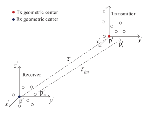
Figure 27: Localization in a massive MIMO system [83].

V-A3 RSS-based Localization

RSS is also a popular signal metric for localization, especially in fingerprinting-based and proximity-based localization schemes [88, 89]. For narrowband signals, attenuation of the signal strength through a mobile radio channel is caused by three nearly independent factors: path loss, log-normal shadowing, and multipath fading (or fast fading). In RSS-based localization, time-averaging is commonly used to estimate the mean received signal strength. For wideband signals, the mean signal strength is evaluated by summing powers of multipath in a power delay profile. The mean signal strength is conventionally modeled in dB scale as

$$P=P_{0}-10\alpha\log_{10}d_{n}+e_{RSS,n},$$ (63)

$$d_{n}=\sqrt{\left(x_{n}-x\right)^{2}+\left(y_{n}-y\right)^{2}},n=1,2,...,N_{{\rm b}},$$ (64)

where $\left(x_{n},y_{n}\right)$ denotes the known position of anchor $n$, $\left(x,y\right)$ denotes the agent’s position, $e_{RSS,n}\sim\mathcal{N}\left(0,\eta_{n}^{2}\right)$ is a Gaussian random variable representing the log-normal fading, and $\alpha$ is the path loss exponent.

The squared position error bound (SPEB) of the RSS-based localization is expressed as

$$\left(\frac{\ln 10}{10\alpha}\right)^{2}\frac{\sum_{i=1}^{N_{\mathrm{b}}}\eta_{i}^{-2}d_{i}^{-2}}{\sum_{i=1}^{N_{\mathrm{b}}}\sum_{j=1}^{i-1}\eta_{i}^{-2}\eta_{j}^{-2}d_{i}^{-2}d_{j}^{-2}\sin^{2}\left(\phi_{i}-\phi_{j}\right)},$$ (65)

where $\phi_{i}=\tan^{-1}\frac{y-y_{i}}{x-x_{i}}$ is the angle determined by the positions of $i$-th anchor and the agent. As can be observed from (65), the accuracy of RSS-based localization depends heavily on the channel parameters, namely the path loss exponent $\alpha$ and the shadowing variances $\eta_{n}^{2}$, wherein the SPEB is proportional to $\eta_{n}^{2}$ and inversely proportional to the square of $\alpha$. Furthermore, the effects of NLOS propagation are implicitly included in the RSS signal model.

V-A4 Hybrid Scheme

Besides the schemes using a single signal metric for localization, many hybrid schemes have been proposed for localization. In [90], the author derived the CRB based on hybrid RSS-TOA measurements. [91] derived the CRB based on a hybrid DOA-TOA localization scheme. Moreover, for the purpose of eliminating the dependence of estimation accuracy to the specific anchors’ geolocation, the anchor locations were modeled as Poisson Point Processes (PPP) in [92] to study the average localization performance over the spatial PPP distribution. The derived average CRB bound acts on the expectation of the MSE with respect to the random anchor locations depending on the network statistics.

In the following, we elaborate the CRB analysis in [91] for the hybrid DOA-TOA localization scheme. Consider a far-field scenario with single-path LOS propagation where the agent is equipped with an uniform linear array (ULA) of $N$ elements for receiving the reference signal from an anchor with a single transmit antenna. First, the CRB of TOA and DOA estimates are derived respectively as follows:

$$\mathrm{CRB}_{\tau}=\frac{1}{8\pi^{2}N\textrm{SNR}\beta^{2}},$$ (66)

$$\mathrm{CRB}_{\theta}=\frac{3\lambda^{2}}{4\pi^{2}d^{2}\textrm{SNR}\cos^{2}\theta(N-1)N(2N-1)},$$ (67)

where $\beta^{2}$ denotes the squared effective bandwidth of the unit-energy transmitted signal $s\left(t\right)$, $d$ is the antenna element separation, $\theta$ is the DOA and $\lambda$ is the wavelength of the planewave signal. Apparently, the CRB of TOA is dominantly determined by the effective bandwidth $\beta$, while that of DOA is mainly affected by array configuration parameters $N$ and $d$.

Then, the CRB of the location estimate is derived based on that of the TOA and DOA estimates according to the chain rule. The relation can be written as

$$\begin{array}[]{l}\mathrm{CRB}_{x}=c^{2}\tau^{2}\cos^{2}\theta\mathrm{CRB}_{\theta}+c^{2}\sin^{2}\theta\mathrm{CRB}_{\tau}\\ \mathrm{CRB}_{y}=c^{2}\tau^{2}\sin^{2}\theta\mathrm{CRB}_{\theta}+c^{2}\cos^{2}\theta\mathrm{CRB}_{\tau}\end{array},$$ (68)

where $\mathrm{CRB}_{x}$ and $\mathrm{CRB}_{y}$ denote the CRB of the agent position in x-axis and y-axis of the 2-D plane. The MMSE of the location estimate is given by

$$\mathrm{MMSE}=\mathrm{CRB}_{x}+\mathrm{CRB}_{y}=c^{2}\tau^{2}\mathrm{CRB}_{\theta}+c^{2}\mathrm{CRB}_{\tau}.$$ (69)

From the final result, we can conclude that the location accuracy depends on the SNR, antenna element number, antenna element separation, squared effective bandwidth, and the relative position between the anchor and the agent. When the relative distance $c\tau$ is large, the destructive effect of the estimation errors of DOA for localization will be magnified.

V-B Cooperative Wireless Localization

V-B1 Spatial cooperation

In spatial cooperation, the agents also transmit reference signals to aid the localization of the neighbor agents. In this case, the localization accuracy of all agents can be potentially enhanced. A few works have studied the fundamental limits of spatial cooperation. In [93], the authors derived the performance bound based on the signal metrics (e.g., TOA and DOA) extracted from the received signals. However, such performance bound may not be the fundamental limit since signal metrics may not contain all useful information for localization. Hence in [82], the authors extended their prior work [78] to the spatial cooperation scenario and derived more general fundamental limits of cooperative wireless localization based on received waveforms rather than signal metrics. Furthermore, in [94], the authors considered an anchorless cooperative localization scenario for diminishing the effect of network topology on the performance bound. Under this assumption, the localization performance is mainly determined by the number of nodes in the network and the signal metric used. Also, in [95], the authors considered an AOA-based cooperative localization scheme.

For the scenario of spatial cooperation, the EFIM and RI method introduced in [78] can also be applied similar to the non-cooperative scenario for whatever the signal metric used, e.g., TOA, TDOA, AOA, RSS or received waveform itself. Hence, for getting more insights into the cooperative localization, we next present the fundamental limit analysis in [82].

In the spatial cooperation considered in [82], the signal model is the same as (50). The only difference is that the agents also transmit reference signals, i.e., agent $k$ receives localization signals from all the other nodes, including both anchors and the other agents. Suppose there are a set of $N_{a}$ agents denoted as $\mathcal{N}_{a}$ and a set of $N_{b}$ anchors denoted as $\mathcal{N}_{b}$. The EFIM for the agent positions $\mathbf{P}=\left[\begin{array}[]{llll}\mathbf{p}_{1}^{\mathrm{T}}&\mathbf{p}_{2}^{\mathrm{T}}&\cdots&\mathbf{p}_{N_{\mathrm{a}}}^{\mathrm{T}}\end{array}\right]^{\mathrm{T}}$in this case is a $2N_{\mathrm{a}}\times 2N_{\mathrm{a}}$ matrix, which can be written as

$$\mathbf{J}_{\mathrm{e}}(\mathbf{P})=\mathbf{J}_{\mathrm{e}}^{\mathrm{A}}(\mathbf{P})+\mathbf{J}_{\mathrm{e}}^{\mathrm{C}}(\mathbf{P}),$$ (70)

where $\mathbf{J}_{\mathrm{e}}^{\mathrm{A}}(\mathbf{P})$ and $\mathbf{J}_{\mathrm{e}}^{\mathrm{C}}(\mathbf{P})$ denote the information from anchors and agent spatial cooperation respectively.

$$\mathbf{J}_{\mathbf{e}}(\mathbf{P})=\left[\begin{array}[]{cccc}\mathbf{J}_{\mathrm{e}}^{\mathrm{A}}\left(\mathbf{p}_{1}\right)+\sum_{j\in\mathcal{N}_{\mathrm{a}}\backslash\{1\}}\mathbf{C}_{1,j}&-\mathbf{C}_{1,2}&\cdots&-\mathbf{C}_{1,N_{\mathrm{a}}}\\ -\mathbf{C}_{1,2}&\mathbf{J}_{\mathrm{e}}^{\mathrm{A}}\left(\mathbf{p}_{2}\right)+\sum_{j\in\mathcal{N}_{\mathbf{a}}\backslash\{2\}}\mathbf{C}_{2,j}&\cdots&-\mathbf{C}_{2,N_{\mathrm{a}}}\\ \vdots&\vdots&\ddots&\vdots\\ -\mathbf{C}_{1,N_{\mathrm{a}}}&-\mathbf{C}_{2,N_{\mathrm{a}}}&...&\mathbf{J}_{\mathrm{e}}^{\mathrm{A}}\left(\mathbf{p}_{N_{\mathrm{a}}}\right)+\sum_{j\in\mathcal{N}_{\mathrm{a}}\backslash\left\{N_{\mathrm{a}}\right\}}\mathbf{C}_{N_{\mathrm{a}},j}\end{array}\right]$$ (71)

The detailed formulation is given by (71) on the top of the next page, where

$$\begin{array}[]{l}\mathbf{J}_{\mathrm{e}}^{\mathrm{A}}\left(\mathbf{p}_{k}\right)=\sum_{j\in\mathcal{N}_{\mathrm{b}}}\lambda_{k,j}\mathbf{J}_{\mathrm{r}}\left(\phi_{k,j}\right),\\ \mathbf{C}_{k,j}=\mathbf{C}_{j,k}=\left(\lambda_{k,j}+\lambda_{j,k}\right)\mathbf{J}_{\mathbf{r}}\left(\phi_{k,j}\right),j\in\mathcal{N}_{\mathrm{a}}\backslash\{k\},\end{array}$$ (72)

where $\lambda_{k,j}$ is RII corresponding to the reference signal from node $j$ to agent node $k$, $\phi_{k,j}$ is the angle from node $j$ to agent $k$, and ${\bf J}_{\text{r}}\left(\phi\right)$ is the RDM defined in (52).

Note that the RI $\lambda_{k,j}\mathbf{J}_{\mathrm{r}}\left(\phi_{k,j}\right)$ from an anchor node $j$ has the same form of that in the non-cooperation localization, but the RI $\left(\lambda_{k,j}+\lambda_{j,k}\right)\mathbf{J}_{\mathbf{r}}\left(\phi_{k,j}\right)$ from an agent node $j$ is slightly different because the RI between two agent nodes is obtained by measuring the TDOA instead of TOA, since it is difficult to achieve time synchronization between two agents. Nevertheless, the RI is still determined by the SNR and effective bandwidth of the received waveform, and the POC. Also, each RI corresponds to an individual received waveform and is a basic building block of the EFIM. From (71), we can observe that $\mathbf{J}_{\mathrm{e}}^{\mathrm{A}}\left(\mathbf{p}_{k}\right)$ is the sub-matrix in the block-diagonal, which indicates that the localization information from anchors is not interrelated among agents. Besides, $\mathbf{J}_{\mathrm{e}}^{\mathrm{C}}(\mathbf{P})$ is a non block-diagonal matrix, implying that the localization information from agents’ cooperation is highly interrelated. This is expected since the effectiveness of the localization information provided by a particular agent depends on its position error.

V-B2 Spatio-Temporal Cooperation

In [96], the spatial cooperation is further extended into spatio-temporal cooperation, which incorporates the intra-node measurements to further enhance the localization performance by exploiting the temporal correlation of the localization parameters. In this case, the EFIM for the positions can be decomposed into two parts, i.e., the information obtained from spatial cooperation and temporal cooperation. Specifically, the EFIM of spatial cooperation is a block-diagonal matrix of which each block has the same structure as (71). However, the EFIM of temporal cooperation is a non-block-diagonal matrix because the intra-node measurements are relevant to the agent positions at two consecutive instants. A more detailed description can be found in [96].

V-C Summary and Insights

In existing works, CRB and EFIM have been used as the performance metrics for device-based sensing. The two performance metrics are closely related to each other. Specifically, the CRB can be obtained by the inverse of the EFIM. As such, it is in general more difficult to obtain a closed-form expression for the CRB. In this sense, EFIM can better reveal insights about the structure of the information that contributes to the sensing/localization performance. All existing wireless localization schemes explicitly/implicitly utilize three signal metrics for localization, namely, the TOA/TDOA, the AOA and the RSS of the reference signals transmitted over the wireless channel. In all cases, the localization performance improves with the increase of SNR (power resource) and the number of antennas (spatial resource), since the increase of these system resources increases the effective SNR and the number of observations for parameter estimation.

Specifically, in TOA-based schemes, the localization accuracy is affected by the network topology, multipath environment, the signal effective bandwidth, the SNR at the receiver, the NLOS condition, and the prior information about channel parameters or the agent’s position. When there are $M$ transmit antennas at the anchor with a fixed per antenna transmit power, $N$ receive antennas at the agent, and only two paths with delays $\tau_{1}$ and $\tau_{2}$ in the multipath environment, the order of the CRB for the intermediate TOA parameter $\tau_{1}$ associated with each anchor-agent link is given by

$$\mathrm{CRB}_{\tau_{1}}=O\left(\frac{1}{\left(1-\rho\left(\left|\tau_{1}-\tau_{2}\right|\right)\right)MN\beta^{2}{\rm\mathit{\textrm{SNR}}}}\right),$$ (73)

where $\rho\left(\left|\tau_{1}-\tau_{2}\right|\right)$ denotes a function of relative delay $\left|\tau_{1}-\tau_{2}\right|$, $\beta$ denotes the effective bandwidth, SNR denotes the receive SNR of the first path. Compared to the case of single-target device-free sensing using MIMO radar, there is a slight difference since the CRB of delay for different paths is coupled as reflected in the term $\rho\left(\left|\tau_{1}-\tau_{2}\right|\right)$. A similar coupling term also exists in the multi-target device-free sensing case between the parameters of different targets.

In AOA-based schemes and under narrowband assumption, the localization accuracy is affected by the the sample-variances of the transmit and receive antenna positions $\sigma_{T}^{2}$ and $\sigma_{R}^{2}$, the SNR at the receiver, and the antenna element number. When the anchor is equipped with a ULA of $M$ transmit antennas and the agent is equipped with a ULA of $N$ receive antennas, the order of the CRB for the intermediate AOA parameter $\theta$ associated with each anchor-agent link is given by

$$\mathrm{CRB}_{\theta}=O\left(\frac{1}{MN\cos^{2}\theta{\rm\mathit{\textrm{SNR}}}\left(\sigma_{T}^{2}+\sigma_{R}^{2}\right)}\right).$$ (74)

From (74), we can observe that AOA estimation accuracy depends on geometric relation among the agents and the anchors. When the antenna array and the target happen to lie on a straight line, e.g., $\theta=\frac{\pi}{2}$, the CRB will become infinitely large. Note that the CRB order of the AOA parameter is the same as that of the MIMO radar with a single radar pulse (i.e., $L=1$). In (73) and (74), we have assumed that the anchor has no prior information about the agent position and thus there is no transmit beamforming gain tawards the agent. With perfect transmit beamforming tawards the agent, the CRB in (73) and (74) can be reduced by an additional factor of $M$.

In RSS-based schemes, the localization accuracy is affected by the network topology, propagation environment, e.g., path loss exponent and shadowing effects, and the distance between the agent and the anchor.

When multiple signal metrics are used for localization, the estimation accuracy for the agent position will be improved. Furthermore, cooperation among agents can significantly improve localization accuracy and reduce localization outage probabilities, and the localization information from agents’ cooperation is highly interrelated. Agent can treat the information coming from anchors and other cooperating agents in a unified way, since anchors can be seen as an agent with infinite prior position knowledge. Moreover, no matter what kind of cooperation is, the EFIM of the agent position can be expressed as a weighted sum of RDMs, and the weight is called the RII, which measures the strength of the information from a node at a specific direction.

VI Information-Theoretic Limits of ISAC

In this section, we present information-theoretic modeling and capacity-distortion tradeoff limits for several important ISAC building blocks. We start with a few studies on device-free ISAC and then move on to the studies on device-based ISAC.

VI-A Capacity-distortion tradeoff for device-free ISAC memoryless channels

In the device-free ISAC systems, the sensing node, equipped with a mono-static/bi-static radar, wishes to transmit/receive message to/from its intended receivers/transmitters and simultaneously estimate the state parameters of interest upon observing the echo signal. By viewing this echo signal as generalized feedback, References [72, 19, 97], have proposed information-theoretic models for several device-free ISAC building blocks and investigated the corresponding capacity-distortion tradeoff.

VI-A1 Device-free ISAC over Memoryless Point-to-Point Channels with Mono-static Sensing

Reference [72] first considered a point-to-point channel with mono-static sensing, where the ISAC transmitter wishes to send message $W$ to the receiver while simultaneously estimating the channel state via output feedback, as illustrated in Fig. 28. The output feedback can be used to model the radar echo signals in practice. Assume that the channel is memoryless with i.i.d. state sequence $s^{n}$ (the $i$-th element $s_{i}\in{\mathcal{S}}$) in a coding block of length $n$, and the receiver knows the state sequence. With input/output alphabet ${\mathcal{X}},{\mathcal{Y}}$ and ${\mathcal{Z}}$, given input $X_{i}=x\in{\mathcal{X}}$, the channel produces outputs $(Y_{i},Z_{i})\in{\mathcal{Y}}\times{\mathcal{Z}}$ according to a given transition law $P_{YZ|XS}(.,.|x,s)$ for each time instance $i$.

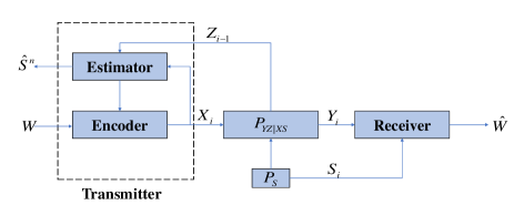
Figure 28: The system model of point-to-point channel with mono-static sensing (generalized feedback).

For this channel model, the capacity-distortion tradeoff has been established in [72, Theorem 1]:

$$C(D)=\max_{P_{X}:\frac{1}{n}\sum_{i}\mathbb{E}\left[\left|X_{i}\right|^{2}\right]\leq P}I(X;Y|S),\text{ s.t. }\mathbb{E}[d(S,\hat{S})]\leq D$$ (75)

where the maximum is taken over all input distributions $P_{X}$ satisfying the average distortion $\mathbb{E}[d(S,\hat{S})]\leq D$, and the joint distribution of ${SXYZ\hat{S}}$ is factorized as

$$P_{SXYZ\hat{S}}(s,x,y,z,\hat{s})$$

$$= P_{S}(s)P_{X}(x)P_{YZ|XS}(y,z|x,s)P_{\hat{S}|XZ}(\hat{s}|x,z)$$ (76)

The estimator $P_{\hat{S}|XZ}(\hat{s}|x,z)$ for $S$ is chosen such that $\mathbb{E}[d(S,\hat{S})]$ is minimized for given input distribution $P_{X}$. It can be seen that the optimal input is constrained by the estimation distortion required. In the case of unconstrained distortion (i.e., $D=\infty$), the result above reduces to the capacity for a memoryless channel with i.i.d. random states where the state is available only at the receiver.

To further illustrate the capacity-distortion tradeoff, consider the following fading channel:

$$Y_{i}=S_{i}X_{i}+N_{i},i=1,\cdots,n,$$ (77)

where $X_{i}$ is the input satisfying average power constraint $\frac{1}{n}\sum_{i}\mathbb{E}\left[\left|X_{i}\right|^{2}\right]\leq P$ and both $S_{i}$ and $N_{i}$ are i.i.d. Gaussian with zero mean and unit variance. The generalized feedback is assumed to be perfect, i.e, $Z=Y$.

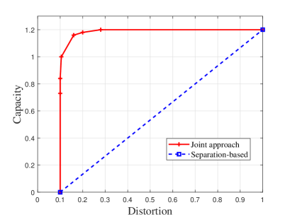
Figure 29: The capacity-distortion tradeoff when $P=10$ dB [72].

Fig. 29 plots the capacity-distortion tradeoff when $P=10$ dB. On one extreme, when $D=1$, $C(D=1)$ reduces to the unconstrained capacity (note that the distortion $D=1$ can be achieved by setting $\hat{S}=0$ no matter what the input distribution is), while on the other extreme, when $D=0$, positive capacity $C(D=0)=0.733$ bcu is still achievable. In general the joint transmission design as proposed in [72] outperforms a communication and sensing separation-based approach.

VI-A2 Device-free ISAC over Memoryless Multiple-Access Channels with Mono-static Sensing

Reference [19] instead considered a two-user multiple-access channel where the $k$-th ($k=1,2$) ISAC transmitter wishes to send message $W_{k}$ to the receiver while simultaneously estimating its channel state via output feedback, as illustrated in Fig. 30. The channel is memoryless with i.i.d. state sequence $s_{k}^{n}$ ($s_{k,i}\in\mathcal{S}_{k}$) in a coding block, and the receiver knows both $s_{1}^{n}$ and $s_{2}^{n}$. With input/output alphabet $\mathcal{X}_{k},Y$ and $\mathcal{Z}_{k}$, given input $X_{k,i}=x\in\mathcal{X}_{k}$, the channel produces outputs $(Y_{i},Z_{1,i},Z_{2,i})\in\mathcal{Y}\times\mathcal{Z}_{1}\times\mathcal{Z}_{2}$ according to a given transition law $P_{YZ_{1}Z_{2}|X_{1}X_{2}S_{1}S_{2}}(.,.,.|x_{1},x_{2},s_{1},s_{2})$ for each time instance $i$.

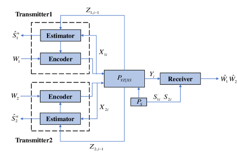
Figure 30: The system model of multiple-access channel with mono-static sensing.

For this ISAC MAC model, outer and inner bounds on the capacity-distortion region have been established, see Theorem 1 and Theorem 2 of [19]. The inner bound exploits the feedback-induced cooperation between the transmitters and is achieved by block Markov encoding and backward decoding, in which three auxiliary random variables $U,V_{1},V_{2}$ are introduced. Specifically, $U$ is the common decoded message from the previous coding blocks through feedback $Z_{1},Z_{2}$, $V_{1}$ is the partial message transmitted by the current coding block of user 1 which can be decoded by user $2$ through feedback $Z_{2}$, and $V_{2}$ is the partial message transmitted by the current coding block of user 2 which can be decoded by user $1$ through feedback $Z_{1}$. Consequently, the estimation of $s_{1}$ at Transmitter $1$ is based on $x_{1}$, $v_{2}$, $z_{1}$ and the optimal estimator $\psi_{1}^{*}\left(x_{1},v_{2}\text{,}z_{1}\right)$ for $S_{1}$ is given by

$$\psi_{1}^{*}\left(x_{1},v_{2}\text{,}z_{1}\right) =\arg\underset{\psi_{1}}{\min}\underset{s_{1}\in\mathcal{S}_{1}}{\sum}P_{S_{1}\mid X_{1}V_{2}Z_{1}}\left(s_{1}\mid x_{1}v_{2}z_{1}\right)$$

$$\times d_{1}\left(s_{1},\psi_{1}\left(x_{1},v_{2},z_{1}\right)\right)$$ (78)

where $d_{1}$ is the distortion function at Transmitter $1$. Given $X_{1}=x_{1},V_{2}=v_{2}$, the estimation cost for $S_{1}$ is

$$c_{1}(x_{1},v_{2})=\mathbb{E}\left[d_{1}\left(s_{1},\psi_{1}^{*}\left(x_{1},v_{2},z_{1}\right)\right)\mid X_{1}=x_{1},V_{2}=v_{2}\right]$$ (79)

The optimal estimator $\psi_{2}^{*}\left(x_{2},v_{1}\text{,}z_{2}\right)$ for $S_{2}$ and the corresponding estimation cost $c_{2}(x_{2},v_{1})$ can be obtained similarly.

For given average distortion constraints $\mathbb{E}[c_{1}(X_{1},V_{2})]\leq D_{1},\mathbb{E}[c_{2}(X_{2},V_{1})]\leq D_{2}$, the inner bound $\mathcal{R}(D_{1},D_{2})$ achieved by the above block Markov encoding and backward decoding scheme consists of all rate pairs $(R_{1},R_{2})$ satisfying

$$R_{1} \leq I\left(X_{1};Y\mid X_{2}V_{1}US\right)+I\left(V_{1};Z_{2}\mid X_{2}U\right)$$

$$R_{2} \leq I\left(X_{2};Y\mid X_{1}V_{2}US\right)+I\left(V_{2};Z_{1}\mid X_{1}U\right)$$

$$R_{1}+R_{2} \leq\begin{array}[]{l}\min\{I\left(X_{1}X_{2};Y\mid S\right),I\left(X_{1}X_{2};Y\mid SV_{1}V_{2}U\right)\\ +I\left(V_{1};Z_{2}\mid X_{2}U\right)+I\left(V_{2};Z_{1}\mid X_{1}U\right)\}\end{array},$$ (82)

where $V_{1}X_{1}-U-V_{2}X_{2}$ and $UV_{1}V_{2}-X_{1}X_{2}-YZ_{1}Z_{2}$ form Markov chains.

To gain insights on the resultant rate-distortion tradeoff, consider the following state-dependent MAC channel:

$$Y=S_{1}X_{1}+S_{2}X_{2},$$ (83)

with binary input $X_{1}$ and $X_{2}$, i.i.d. states $S_{1}$ and $S_{2}$ Bernoulli distributed with parameter $p(s_{k}=1)=p_{s}$ and output feedback $Z_{1}=Z_{2}=Y$.

Fig. 31 plots the sum rate-distortion tradeoff when $D_{1}=D_{2}=D$ and $p_{s}=0.7$, where the x-axis denotes the distortion and the y-axis denotes the sum capacity. There exists gap between the inner bound and the outer bound, however, when the distortion is small, the proposed scheme achieves near-optimal performance. In general the joint transmission design as proposed outperforms a communication and sensing resource sharing approach.

Figure 31: Tradeoff between sum rate and distortion for $p_{s}=0.7$ [19].

VI-A3 Device-free ISAC over Memoryless Broadcast Channels

A more recent work [97] studied a two-user broadcast channel where the ISAC transmitter wishes to send message $W_{k}$ to the $k$-th ($k=1,2$) receiver while simultaneously estimating its channel state via output feedback, as illustrated in Fig. 32. The channel is memoryless with i.i.d. state sequence $s_{k}^{n}$ ($s_{k,i}\in\mathcal{S}_{k}$) in a coding block, and each receiver knows its own state sequence $s_{k}^{n}$. With input/output alphabet $\mathcal{X},\mathcal{Y}_{k}$ and $\mathcal{Z}_{k}$, given input $X_{i}=x\in\mathcal{X}$, the channel produces outputs $(Y_{1,i},Y_{2,i},Z_{1,i},Z_{2,i})\in\mathcal{Y}_{1}\times\mathcal{Y}_{2}\times\mathcal{Z}_{1}\times\mathcal{Z}_{2}$ according to a given transition law $P_{Y_{1}Y_{2}Z_{1}Z_{2}|XS_{1}S_{2}}(.,.,.,.|x,s_{1},s_{2})$ for each time instance $i$.

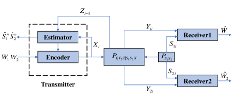
Figure 32: The system model of broadcast channel with mono-static sensing.

In [97], the capacity-distortion tradeoff region was fully characterized for the physically degraded ISAC broadcast channel. In addition, outer and inner bounds on the tradeoff region was established for the general ISAC broadcast channel. As an example of the physically degraded case, consider the following broadcast channel with multiplicative binary states:

$$Y_{k}=XS_{k},~{}~{}k=1,2,$$ (84)

where the joint state probability mass function $P(S_{1}=0,S_{2}=0)=1-q$, $P(S_{1}=0,S_{2}=1)=0$, $P(S_{1}=1,S_{2}=1)=q\gamma$ and $P(S_{1}=1,S_{2}=0)=q(1-\gamma)$ with $q,\gamma\in[0,1]$, and output feedback $Z=(Y_{1},Y_{2})$. The capacity-distortion tradeoff region is depicted in [97, Fig. 2] for $\gamma=0.5$ and $q=0.6$. Again in general the joint transmission design as proposed outperforms a resource-sharing (or separation-based) approach that splits the resource either for sensing or communication.

VI-B Capacity-Distortion Tradeoff for Device-based ISAC Memoryless Channels

For the device-based ISAC system, the receiver aims to simultaneously decode the message and estimate some random parameters of interest from its received signal. By modeling the parameter as a random state, [20] presented an information-theoretic framework of joint communication and state estimation.

Consider a point-to-point memoryless channel. With input/output alphabet $\mathcal{X}$ and $\mathcal{Y}$, given input $X_{i}=x\in\mathcal{X}$, the channel produces output $Y_{i}\in\mathcal{Y}$ according to a given transition law $P_{Y|XS}(.|x,s)$ for each time instance $i$. Assume that the state sequence $s^{n}$ to be estimated is i.i.d with $P(s^{n})=\prod\nolimits_{i=1}^{n}p_{S}\left(s_{i}\right)$ and is unknown to the transmitter. For the model considered, the capacity-distortion function is established in Theorem 1 of [20].

$$C\left(D\right)=\underset{P_{X}\in\mathcal{P}_{D}}{max}I\left(X;Y\right),$$ (85)

where $\mathcal{P}_{D}=\left\{P_{X}:\underset{x\in\mathcal{X}}{\sum}P_{X}\left(x\right)d^{*}\left(x\right)\leq D\right\}$. Here, $d^{*}(x)$ is the estimation cost function due to signaling with $x\in\mathcal{X}$. In other words, $d^{*}(x)$ is the minimum distortion that can be achieved for a given signaling $x\in\mathcal{X}$. $\mathcal{P}_{D}$ regulates the input distribution so that the signaling is estimation-efficient. When $D=\infty$, $C(D)$ reduces to the classic unconstrained channel capacity.

To gain insights on the resultant capacity-distortion tradeoff here, consider the following state-dependent Gaussian channel [20]:

$$Y_{i}=X_{i}+S_{i}+Z_{i},$$ (86)

where $S_{i}\sim\mathcal{\mathcal{C}N}(0,Q)$, $Z_{i}\sim\mathcal{C}N(0,N)$ and $X_{i}$ is subject to an average power constraint $P$. The system achieves the following tradeoff

$$C\left(D\right)=\begin{cases}\begin{array}[]{c}\log\left(1+\frac{P}{Q+N}\right)\\ 0\end{array}&\begin{array}[]{c}D>\frac{QN}{Q+N}\\ D\leq\frac{QN}{Q+N}\end{array}\end{cases}.$$ (87)

It can be seen that a non-zero communication rate is achieved only when the estimation distortion required is not very stringent and above the threshold $QN/(Q+N)$. This demonstrates the cost of achieving finer estimation at the receiver.

The study is also extended to a two-user multiple access channel with device-based sensing and the corresponding capacity-distortion region is the union of all rate pairs $(R_{1},R_{2})$ satisfying

$$R_{1}\leq I\left(X_{1};Y\mid X_{2},Q\right),$$

$$R_{2}\leq I\left(X_{2};Y\mid X_{1},Q\right),$$

$$R_{1}+R_{2}\leq I\left(X_{1},X_{2};Y\mid Q\right),$$ (88)

over $P_{Q}(q)P_{X_{1}|Q}(x_{1}|q)P_{X_{2}|Q}(x_{2}|q)P_{Y|X_{1},X_{2}}(y|x_{1},x_{2})$ that satisfies

$$D\geq\underset{\left(q,x_{1},x_{2}\right)}{\sum}P_{Q}\left(q\right)P_{X_{1}\mid Q}\left(x_{1}\mid q\right)P_{X_{2}\mid Q}\left(x_{2}\mid q\right)d^{*}\left(x_{1},x_{2}\right).$$ (89)

VI-C Summary

Information-theoretic state-dependent channels with generalized output feedback have been shown to be useful in modeling and assessing the performance of device-free ISAC systems. The capacity-distortion tradeoff has been fully characterized for a point-to-point channel under some simplified assumptions, while inner and outer bounds on the capacity-distortion region have been proposed for multiple access and broadcast ISAC channels. The benefit of joint-design approach over separation-based (or resource-sharing) approach is clearly evident. However, the results are derived under some restrictive assumptions, such as the state sequence is i.i.d. or/and channel state and sensing state are the same. New modeling and bounding techniques shall be developed for memoryless device-free ISAC channels under more realistic assumptions.

Similar to device-free ISAC, device-based ISAC also embraces performance tradeoff between communication and sensing. Information-theoretic state-dependent channels with receiver state estimation have been proposed to establish the fundamental capacity-distortion tradeoff in device-based ISAC. In particular, the optimal tradeoff has been fully characterized for a point-to-point channel and a two-user MAC channel with i.i.d. state sequence. This approach can also be generalized and applied to more complicated channel topologies, such as broadcast channels, which are worth further studies.

VII Design and Performance Analysis of Specific ISAC Systems

In this section, we discuss some designs and performance analysis of ISAC systems tailored to different application scenarios. Similar to the previous section, we first focus on the device-free ISAC and then go on to the device-based ISAC.

VII-A Design and Performance Analysis of Some Device-Free ISAC Applications

VII-A1 Application of MAC with Mono-Static BS Sensing

The first application considered is a joint radar-communication system as shown in Fig. 33. The base station is sensing $K$ targets of interest while serving an uplink communication user. Therefore, the echo signals reflected by the targets will be superimposed on the uplink communication signal. This is a MAC with mono-static BS sensing. For $K$ targets, the observed complex baseband signal at the BS is given by

$$y\left(t\right)=\sqrt{P_{com}}\alpha_{cu}s_{c}\left(t\right)+\sqrt{P_{rad}}\sum\limits_{k=1}^{K}\alpha_{rk}s_{r}\left(t-\tau_{k}\right)+z\left(t\right),$$ (90)

where $P_{com}$ is the communication transmit power, $P_{rad}$ is the radar transmit power, $\alpha_{cu}$ is the channel gain for the $u$-th user, $\alpha_{rk}$ is the RCS of the $k$-th target, $\tau_{k}$ is the delay of the $k$-th target and $z\left(t\right)$ is the additive Gaussian noise.

Figure 33: An uplink communication system with mono-static BS sensing.

For this application scenario, various resource-sharing schemes that involve bandwidth partitioning and power allocation have been proposed and their associated performance bounds have been established for each scheme, see Section IV. of [98]. Therein, the performance of estimating $\tau_{k}$ is quantified by the notion of estimation information rate as discussed in Section III in this paper. Fig. 34 compares the tradeoffs between communication information rate and estimation information rate under different schemes. Outer bounds on communications and radar are indicated by the red lines. Successive interference cancellation (SIC) bound for the communications rate is indicated by the green dashed line. The linear interpolation between SIC vertex and the radarfree data rate bound is indicated by the gray dashed line. The water-filling inner bound is indicated by the blue line. It can be seen that the water-filling bound generally outperforms the other inner bounds, because it advocates flexible sub-band partitioning (one for communications only and the other for both radar and communications) and optimized power allocation between the sub-bands.

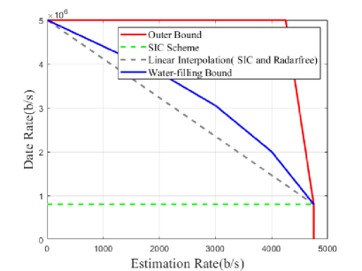
Figure 34: The tradeoffs between communication information rate and estimation information rate under different schemes [98].

VII-A2 Application of Point-to-Point Channel with Mono-Static Sensing

The second application considered is a point-to-point channel with mono-static sensing in vehicular networks as shown in Fig. 35. Specifically, a source vehicle sends an adaptive IEEE 802.11ad single-carrier physical layer frame to a target vehicle and uses the reflections from the target vehicle to derive its range and velocity. Each frame has $K$ symbols in total, with $\alpha=\frac{K_{c}}{K}$ fraction of them for data and the rest for preamble.

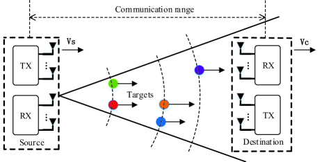
Figure 35: A point-to-point communication system with mono-static sensing.

For the system considered, the effective maximum achievable communication spectral efficiency depends on $\alpha$ and is expressed as

$$r_{\text{eff}}=\alpha\log(1+\text{SNR}_{c})=\log(1+\text{SNR}_{c})^{\alpha},$$ (91)

where $\text{SNR}_{c}$ represents the communication SNR that accounts for the path-loss.

As for sensing, in case of velocity estimation using the preamble of the IEEE 802.11ad frame, the CRB is given by [71]

$$\text{CRB}_{v}=\frac{6\lambda^{2}}{16\pi^{2}\left(1-\alpha\right)^{3}K^{3}T_{s}^{2}\text{SNR}_{r}},$$ (92)

where $\text{SNR}_{r}$ is the radar SNR, $\lambda$ is the wave-length and $T_{s}$ is the symbol duration. On the other hand, the CRB for the range estimation of a target vehicle is given by

$$\text{CRB}_{d}=\frac{c^{2}}{32\pi^{2}B_{\text{rms}}^{2}\left(1-\alpha\right)K\text{SNR}_{r}},$$ (93)

where $B_{\text{rms}}$ is the root-mean square bandwidth of the Fourier transform of the preamble and $c$ is the speed of the light.

It can be seen from (91) - (93) that both radar and communication performance metrics are dependent on $\alpha$. In addition, the communication rate $r_{\text{eff}}$ can be derived to its equivalent MSE metric as $\text{MMSE}_{\text{eff}}=2^{-r_{\text{eff}}}$ as discussed in Section III. Therefore, one can optimize $\alpha$ through the following weighted optimization problem:

$$\mathop{\min}\limits_{\alpha}\omega_{d}\log\left(\text{CRB}_{d}\right)+\omega_{v}\log\left(\text{CRB}_{v}\right)-\omega_{c}\log\left(\text{MMSE}_{\text{eff}}\right)$$

$$~{}~{}~{}~{}~{}~{}~{}~{}~{}~{}~{}~{}~{}~{}~{}\text{s.t.}~{}0\leq\alpha\leq 1,$$ (94)

to achieve the optimal tradeoff between communication and radar sensing performance.

VII-B Design and Performance Analysis of Some Device-Based ISAC Applications

VII-B1 Performance Analysis for Point to Point Communication with Localization

In [99], Armin introduced a parametric positioning waveform design which provides a scalar parameter for controlling the distribution of the PSD. When the single-carrier transmission scheme is considered, the signal which has more power concentrated at the edges of the spectrum leads to a larger equivalent signal bandwidth, resulting a lower CRB in positioning. However, for communication, the optimal signal PSD scheme is to concentrate the signal power at the central of the mainlobes. Consequently, there is a trade-off for waveform design between localization and communication. Besides the study of waveform design, the power-partitioning scheme for satisfying different localization and data-rate requirements is also researched in the millimeter wave network [100]. Ghatak adopted the Bayesian CRLB and Rate Coverage Probability as the performance metrics of localization and communication respectively to be satisfied. Apparently, as more transmit power allocated for data services, the rate coverage probability will improve while the localization accuracy will degrade. In [101], Destino also considered a millimeter wave wireless network, which utilized a beam training period for localization. Different from the RSS measurements used by [100] for localization, the TOA-based beam alignment scheme is considered, which reveals a trade-off between localization accuracy and effective communication rate. Nevertheless, only an exhaustive search strategy is considered and without the consideration of beam misalignment error.

VII-B2 Performance Analysis and Optimization for Multiple Access Communication with Localization

In [102], the prior work [101] is extended to multi-user scenario. The author considered a millimeter wave based multi-user single-input-multiple-output (SIMO) wireless uplink system with an $N$-antenna BS and $U$ single-antenna mobile stations (MSs) as shown in Fig. 36, and orthogonal resource allocation for different MSs is assumed, e.g., by using time-division-multiple-access (TDMA) or frequency-division-multiple-access (FDMA). In this system, a joint localization and data transmission scheme was proposed. In each transmission block of fixed duration $T_{f}$, the training phase of duration $T_{t}$ is used for beam alignment and localization while the data phase of duration $T_{d}$ is used for data transmission as shown in Fig. 37.

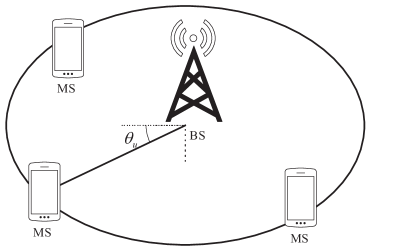
Figure 36: An uplink communication system with localization.

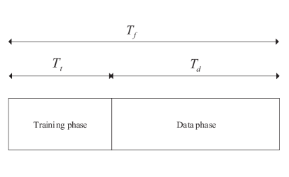
Figure 37: Joint localization and data transmission scheme.

During the training phase, an exhaustive beam alignment strategy is used. Specifically, for each user, the BS sequentially trains each of the beam in the codebook set $\mathcal{W}$ and find the best one that maximizes the beamforming gain of this user. Assuming LOS channels for all users, the received signal at the BS for training the $k$-th MS can be written as

$$y_{k}\left(t\right)=\alpha_{k}\mathbf{w}^{H}\mathscr{\mathbf{a}}_{R}\left(\theta_{k}\right)x_{k}\left(t-\tau_{k}\right)+\mathbf{w}^{H}\mathbf{n}\left(t\right),$$ (95)

where $\alpha_{k}$ and $\theta_{k}$ are the complex gain and AOA associated with the LOS path of the $k$-th MS, $\mathbf{w}\in\mathcal{W}$ is the receive beamforming vector, $\mathscr{\mathbf{a}}_{R}\left(\theta_{k}\right)$ is the receive array response vector with AOA $\theta_{k}$, $x_{k}\left(t\right)$ is the reference signal, $\tau_{k}$ is the delay of the LOS path, and $\mathbf{n}\left(t\right)$ is the additive white Gaussian noise.

For a fixed frame duration $T_{f}$, one can expect that there is a trade-off between communication QoS and localization accuracy, which are quantified by effective data-rate $R_{k}$ and Position Error Bound (PEB) $Q_{k}$

$$R_{k}=B\frac{T_{d}}{T_{f}}f_{k}\log_{2}\left(1+\frac{\mathrm{SNR}_{k}}{f_{k}}\right),$$ (96)

$$Q_{k}=\mathrm{tr\left(\sum_{\mathbf{w}\in\mathcal{W}}\mathbf{J}_{k,\boldsymbol{w}}\right)},$$ (97)

where $f_{k}\in(0,1)$ denotes the fraction of $T_{d}$ resources allocated to the $k$-th MS, $\mathrm{SNR}_{k}$ denotes the receive SNR, $B$ denotes the signal bandwidth, and $\mathbf{J}_{k,\boldsymbol{w}}$ denotes the FIM associated with a single beam $\mathbf{w}$. The PEB is calculated by the summation of the FIM over all beams in codebook set $\mathcal{W}$ used in the exhaustive beam alignment strategy. Since the receive beamforming vector remain fixed for the complete data reception phase, a compromise receive beamforming vector is adopted by the superposition of best receive beam of each MS. Then an optimization problem is formulated to find the optimal resources allocation scheme based on the optimization variables $f_{k}$ and $T_{t}$ with the objective of maximizing the minimum data rate of MSs subject to the PEB constraints.

The simulation results indicate that more time spent for beam training (i.e., larger $T_{t}$) leads to better beam alignment and localization accuracy. However, this would reduce the time left for data transmission (i.e., smaller $T_{d}$). Hence, there exists an optimal training overhead that strikes the balance between the effective achievable sum rate and the localization performance.

VII-B3 Other Performance Analysis

There are other applications that involve broadcasting, relaying or D2D communication, as discussed in Section II. For relay channel with cooperative localization, the relay can assist communication and localization, the typical infrastructure of which is the unmanned aerial vehicles (UAV). The UAV can be located by the ground BSs and then can be used as a new anchor node to assist the terrestrial localization. Meanwhile, the aerial mobile networks can also provide communication services via UAV-aided relaying. Hence, there are two links between the BS and the user, therein the BS-User direct link and the BS-Relay-User link, both of which can provide data communication and positioning functionalities. Apparently, the performance bound for relay channel will be more sophisticated than the single link channel topology. Moreover, the ISAC problem is studied under RIS-aided wireless network, where a beamforming design was studied for integrated localization and communication [103]. In D2D channel topology, the user receives waveforms both from the BS and other neighboring users, which can be either communication signals or localization reference signals. The user needs to achieve accurate positioning by cooperation with other users and D2D communication simultaneously. Different from the relay or RIS aided channel, the indirect link between the BS and the user is connected by another user.

VII-C Summary

The typical application of device-free ISAC is for joint radar and communication. Two specific designs that involve mono-static sensing have been reviewed in this section. Estimation-information-rate induced approach and equivalent-MSE induced approach as presented in Section III have been shown to be useful in establishing bounds on the sensing-communication performance tradoff. On the other hand, the typical application of device-based ISAC is for joint communication and localization. A number of past studies have focused on optimizing the resource allocation in either power, time or spatial domain to strike a good balance between the achievable data rate and localization accuracy. To further improve the performance, the concept of relay-aided (static relay, or mobile relay such as UAV) cooperative communication and localization has also been explored yet in a very preliminary manner. Very few performance limits were reported in this case, which deserves further study.

VIII Open Problems and Future Research Directions

The research on the fundamental limits of device-free and device-based sensing (especially those based on the EFIM and CRB analysis) is relatively mature. However, the fundamental limits of many ISAC scenarios remain open. For example, even for the simplest scenario of point-to-point channel with mono-static sensing, a complete characterization of the communication capacity and sensing distortion region (capacity-distortion region) is still unknown for non-i.i.d. channel/sensing states. There are many other ISAC network topologies that have not been studied before. It is also important to study the fundamental limits under more practical considerations such as the imperfect CSI, frequency offset and timing synchronization error, different mobility models, etc., and optimize the system performance based on the fundamental limits analysis. In the following, we will discuss some of these open problems and future research directions in details.

VIII-A Tighter Information-Theoretical Bounds for Capacity-Distortion Region of ISAC

In classic sensing scenarios, the parameter estimation is performed based on a known waveform send by the transmitter, and the prior distribution of the parameters is given and cannot be controlled by the sensing scheme. In this case, the CRB provides a tight lower bound for the MSE performance of unbiased estimators in the high SNR regime. There also exist other sensing bounds such as Weiss-Weinstein bound (WWB) and Zik-Zakai bound (ZZB), which can provide a tighter lower bound of MSE for moderate and low SNR regimes. However, in ISAC scenarios, the estimation is usually performed based on communication signals, which can be encoded signals. The receiver needs to recover the communication message and the sensor needs to estimate the parameter from the encoded communication signals. In this case, we need to characterize the capacity-distortion region, which is fundamentally different from the classic sensing or communication scenarios. In general, we cannot separately analyze the communication capacity and the sensing performance using the classic bounds such as CRB. We have to derive new inner and outer bounds for the capacity-distortion region, based on novel information-theoretical bounds.

VIII-A1 Tight Bounds for Memoryless ISAC Channels

In Section VI-A, we have presented some existing inner and outer bounds for a few simple memoryless ISAC channels, where both the channel state and sensing state are assumed to be i.i.d. and ergodic over one codeword. However, only in some special cases, the inner and outer bounds coincide with each other and part of the capacity-distortion region can be determined. The optimal achievable scheme and the associated capacity-distortion region remain unknown for most cases. In addition, the current information-theoretical bounds for the memoryless ISAC channels are obtained under some restrictive assumptions. For example, in [72, 19, 97], the channel state and sensing state are assumed to be the same. In [20], the receiver is assumed to know the perfect channel/sensing state. However, in practice, the channel and sensing states are usually different but correlated with each other, and the receiver usually does not have the channel state information to begin with. Therefore, an important future research direction is to derive tighter bounds for memoryless ISAC channels under more realistic assumptions. To achieve this, we need to develop joint sensing and channel coding schemes as well as new bounding techniques that can work with more realistic assumptions (e.g., with different channel and sensing states, and without perfect channel state information at the receiver) and can close the gap between the inner and outer bounds. For example, it is possible to exploit the sensed state at the transmitter to improve the joint sensing and channel coding scheme and improve the achievable region (i.e., inner bounds of the capacity-distortion region).

VIII-A2 Information-Theoretical Bounds for Block-Varying ISAC Channels

In many practical applications, the channel and sensing states are not i.i.d. but block-varying, i.e., the channel/sensing state (approximately) remains constant over one codeword. There still lacks studies on the fundamental limits of such block-varying ISAC channels. One major challenge of characterizing the capacity-distortion region for the block-varying ISAC channel is as follows. In traditional communication scenario, the block-varying ISAC channel reduces to the block fading channel. In this case, the Shannon capacity region is well defined under the assumption of perfect CSI at the transmitter (CSIT). However, in block-varying ISAC channels, it may not make sense to assume perfect CSIT, especially when the communication channel is also part of the sensing channel. In this case, the transmitter may learn some imperfect CSIT via self-sensing or CSI feedback from the receiver. As such, we may need to incorporate the overhead of CSIT acquisition/state sensing and the effect of imperfect CSIT in the analysis of the capacity-distortion region, which is very challenging. In fact, the Shannon capacity may not be well defined under imperfect CSIT. In this case, how to properly define and characterize the capacity-distortion region of block-varying ISAC channels is still an open problem and deserves further study.

VIII-B Fundamental Limits of Emerging ISAC Scenarios

The study of the fundamental limits of ISAC is still at an early stage, and many ISAC scenarios have not been investigated. In the following, we discuss several important ISAC scenarios that have not been considered before.

VIII-B1 More Complicated ISAC Network Topologies

One interesting research direction is to study the fundamental limits for other important ISAC network topologies obtained by merging the sensing network topologies with communication network topologies. For example, we may consider mono-static interference networks where there are multiple communication transmitter-receiver pairs interfering with each other and each communication transmitter also serves as a radar transmitter to detect some moving targets. Furthermore, we may introduce cooperation between the transmitters to enhance both the communication and sensing performance, which is a useful ISAC scenario for 6G cellular networks where the BSs can perform cooperative communication and sensing via backhaul/fronthaul connections.

VIII-B2 Intelligent reflecting surface (IRS) aided ISAC

IRS-aided ISAC is another ISAC scenario deserving further study. The IRS can be used to change the communication/sensing channel and thus has the potential to enhance the communication and sensing performance. For example, the IRS may create NLOS paths with known scatter locations (the IRS serves as a scatter with known location). In this case, the NLOS paths created by the IRS can provide useful information to both localization and communications, and thus enhance the coverage and performance of communication and localization services. In some device-free sensing scenarios, it is possible to equip an IRS at the target surface (e.g., when the target is an autonomous vehicle) to enhance the target estimation performance via passive beamforming at the target IRS. Since the IRS-aided ISAC systems have the ability to adjust the communication/sensing channel through passive beamforming, the analysis of fundamental limits of IRS-aided ISAC systems is completely different from the conventional ISAC systems.

VIII-B3 Environment Side Information aided ISAC

When environment side information such as map information is available, we can exploit this prior information to enhance the performance of ISAC systems. A new information-theoretical framework is needed to incorporate the map information into the fundamental limits analysis.

VIII-C Fundamental Limits of ISAC under Practical Considerations

Most existing works on the fundamental limits of ISAC have ignored some important practical issues, such as the channel estimation error, the frequency offset and timing synchronization error, the mobility, etc. In the following, we shall point out several important practical issues that should be taken into account in future studies.

VIII-C1 Channel Estimation Error

In practice, the channel state information is never perfect due to the channel estimation error, CSI feedback delay and CSI quantization error. As already mentioned before, it is important to study how to incorporate the overhead of CSI acquisition and the effect of imperfect CSI in the analysis of fundamental limits of ISAC.

VIII-C2 Frequency Offset and Timing Synchronization Error

Due to the hardware impairments, there always exist frequency offset and timing synchronization error between different sensing or communication transceivers. Unlike the traditional communication systems which have relatively low requirement on the frequency offset and timing synchronization error, the sensing performance of ISAC is very sensitive to the frequency offset and timing synchronization error especially for future ISAC systems with a high requirement on the sensing accuracy. For example, 6G communication systems are expected to achieve a positioning accuracy at the subcentimeter level [104]. In this case, a small timing synchronization error of 0.1 nanosecond will lead to a localization error of several centimeters. Therefore, the future ISAC systems must take this problem into account. We notice that several works have studied the fundamental limits of radar sensing/localization under the consideration of frequency offset and timing synchronization error [96], which is however, not the case for ISAC.

VIII-C3 Tracking Performance Analysis under Different Mobility Models

The channel and sensing states usually change smoothly over time following certain dynamics induced by the mobility pattern. Therefore, it is of great importance to study the tracking performance of channel/sensing state under different mobility models. Some initial tracking performance analysis has been conducted in [56] for visible light-based positioning, where the conditions under which the tracking process is stable (i.e., the state tracking error is bounded as time goes to infinity) is derived, and the converged state error is also analyzed. We may leverage the tools therein and study the fundamental tracking performance limits in more general ISAC systems.

IX Conclusions

In this work, a survey of recent studies on the fundamental limits of integrated sensing and communication has been provided. According to whether the sensing targets participating the sensing procedure by transmitting and/or receiving, we first classify the ISAC related technologies into four major categories: device-free sensing, device-based sensing, device-free ISAC and device-based ISAC, and then each category is further divided into different cases. For each case, we highlight several important works, and present the system model, performance bounds and key insights learned from the analysis of the fundamental limits. In particular, we propose several typical ISAC channel topologies as abstracted models for various ISAC systems, and present the current research progress on the fundamental limits for each ISAC channel. We show that the fundamental limits of ISAC channels cannot be obtained by a trivial combinations of existing performance bounding techniques in separate sensing and communication systems. Finally, we present a list of important open challenges and potential research directions on ISAC, many of them have not been mentioned in the previous works.

References

- [1] B. Paul, A. R. Chiriyath, and D. W. Bliss, “Survey of rf communications and sensing convergence research,” IEEE Access, vol. 5, pp. 252–270, 2017.
- [2] O. B. Akan and M. Arik, “Internet of radars: Sensing versus sending with joint radar-communications,” IEEE Communications Magazine, vol. 58, no. 9, pp. 13–19, 2020.
- [3] F. Liu, C. Masouros, A. P. Petropulu, H. Griffiths, and L. Hanzo, “Joint radar and communication design: Applications, state-of-the-art, and the road ahead,” IEEE Transactions on Communications, vol. 68, no. 6, pp. 3834–3862, 2020.
- [4] Z. Feng, Z. Fang, Z. Wei, X. Chen, Z. Quan, and D. Ji, “Joint radar and communication: A survey,” China Communications, vol. 17, no. 1, pp. 1–27, 2020.
- [5] O. B. Akan and M. Arik, “Internet of radars: Sensing versus sending with joint radar-communications,” IEEE Communications Magazine, vol. 58, no. 9, pp. 13–19, 2020.
- [6] K. Zheng, Q. Zheng, H. Yang, L. Zhao, L. Hou, and P. Chatzimisios, “Reliable and efficient autonomous driving: the need for heterogeneous vehicular networks,” IEEE Communications Magazine, vol. 53, no. 12, pp. 72–79, 2015.
- [7] I. Bilik, O. Longman, S. Villeval, and J. Tabrikian, “The rise of radar for autonomous vehicles: Signal processing solutions and future research directions,” IEEE Signal Processing Magazine, vol. 36, no. 5, pp. 20–31, 2019.
- [8] T. Huang, N. Shlezinger, X. Xu, Y. Liu, and Y. C. Eldar, “Majorcom: A dual-function radar communication system using index modulation,” IEEE Transactions on Signal Processing, vol. 68, pp. 3423–3438, 2020.
- [9] P. Kumari, S. A. Vorobyov, and R. W. Heath, “Adaptive virtual waveform design for millimeter-wave joint communication-radar,” IEEE Transactions on Signal Processing, vol. 68, pp. 715–730, 2020.
- [10] Y. Liu, G. Liao, J. Xu, Z. Yang, and Y. Zhang, “Adaptive ofdm integrated radar and communications waveform design based on information theory,” IEEE Communications Letters, vol. 21, no. 10, pp. 2174–2177, 2017.
- [11] F. Liu, C. Masouros, T. Ratnarajah, and A. Petropulu, “On range sidelobe reduction for dual-functional radar-communication waveforms,” IEEE Wireless Communications Letters, vol. 9, no. 9, pp. 1572–1576, 2020.
- [12] M. Jamil, H. Zepernick, and M. I. Pettersson, “On integrated radar and communication systems using oppermann sequences,” in MILCOM 2008 - 2008 IEEE Military Communications Conference, 2008, pp. 1–6.
- [13] X. Li, R. Yang, Z. Zhang, and W. Cheng, “Research of constructing method of complete complementary sequence in integrated radar and communication,” in 2012 IEEE 11th International Conference on Signal Processing, vol. 3, 2012, pp. 1729–1732.
- [14] A. Pezeshki, A. R. Calderbank, W. Moran, and S. D. Howard, “Doppler resilient golay complementary waveforms,” IEEE Transactions on Information Theory, vol. 54, no. 9, pp. 4254–4266, 2008.
- [15] W. Yuan, F. Liu, C. Masouros, J. Yuan, D. W. K. Ng, and N. González-Prelcic, “Bayesian predictive beamforming for vehicular networks: A low-overhead joint radar-communication approach,” IEEE Transactions on Wireless Communications, pp. 1–1, 2020.
- [16] C. Shi, F. Wang, S. Salous, and J. Zhou, “Joint subcarrier assignment and power allocation strategy for integrated radar and communications system based on power minimization,” IEEE Sensors Journal, vol. 19, no. 23, pp. 11 167–11 179, 2019.
- [17] F. Liu, C. Masouros, A. Li, H. Sun, and L. Hanzo, “Mu-mimo communications with mimo radar: From co-existence to joint transmission,” IEEE Transactions on Wireless Communications, vol. 17, no. 4, pp. 2755–2770, 2018.
- [18] J. Wang, X. Liang, L. Chen, L. Wang, and K. Li, “First demonstration of joint wireless communication and high-resolution sar imaging using airborne mimo radar system,” IEEE Transactions on Geoscience and Remote Sensing, vol. 57, no. 9, pp. 6619–6632, 2019.
- [19] M. Kobayashi, H. Hamad, G. Kramer, and G. Caire, “Joint state sensing and communication over memoryless multiple access channels,” in 2019 IEEE International Symposium on Information Theory (ISIT), 2019, pp. 270–274.
- [20] W. Zhang, S. Vedantam, and U. Mitra, “Joint transmission and state estimation: A constrained channel coding approach,” IEEE Transactions on Information Theory, vol. 57, no. 10, pp. 7084–7095, 2011.
- [21] M. Hurtado, J. Xiao, and A. Nehorai, “Target estimation, detection, and tracking,” IEEE Signal Processing Magazine, vol. 26, no. 1, pp. 42–52, 2009.
- [22] M. Z. Win, Y. Shen, and W. Dai, “A theoretical foundation of network localization and navigation,” Proceedings of the IEEE, vol. 106, no. 7, pp. 1136–1165, 2018.
- [23] C. Laoudias, A. Moreira, S. Kim, S. Lee, L. Wirola, and C. Fischione, “A survey of enabling technologies for network localization, tracking, and navigation,” IEEE Communications Surveys Tutorials, vol. 20, no. 4, pp. 3607–3644, 2018.
- [24] G. Han, J. Jiang, C. Zhang, T. Q. Duong, M. Guizani, and G. K. Karagiannidis, “A survey on mobile anchor node assisted localization in wireless sensor networks,” IEEE Communications Surveys Tutorials, vol. 18, no. 3, pp. 2220–2243, 2016.
- [25] I. Guvenc and C. Chong, “A survey on toa based wireless localization and nlos mitigation techniques,” IEEE Communications Surveys Tutorials, vol. 11, no. 3, pp. 107–124, 2009.
- [26] A. Yassin, Y. Nasser, M. Awad, A. Al-Dubai, R. Liu, C. Yuen, R. Raulefs, and E. Aboutanios, “Recent advances in indoor localization: A survey on theoretical approaches and applications,” IEEE Communications Surveys Tutorials, vol. 19, no. 2, pp. 1327–1346, 2017.
- [27] D. Wu, D. Zhang, C. Xu, H. Wang, and X. Li, “Device-free wifi human sensing: From pattern-based to model-based approaches,” IEEE Communications Magazine, vol. 55, no. 10, pp. 91–97, 2017.
- [28] B. Tan, Q. Chen, K. Chetty, K. Woodbridge, W. Li, and R. Piechocki, “Exploiting wifi channel state information for residential healthcare informatics,” IEEE Communications Magazine, vol. 56, no. 5, pp. 130–137, 2018.
- [29] M. L. Rahman, J. A. Zhang, K. Wu, X. Huang, Y. J. Guo, S. Chen, and J. Yuan, “Enabling joint communication and radio sensing in mobile networks–a survey,” arXiv preprint arXiv:2006.07559, 2020.
- [30] C. Hülsmeyer, “The telemobiloscope,” Electrical Magazine, vol. 2, p. 388, 1904.
- [31] E. Fishler, A. Haimovich, R. Blum, D. Chizhik, L. Cimini, and R. Valenzuela, “Mimo radar: an idea whose time has come,” in Proceedings of the 2004 IEEE Radar Conference (IEEE Cat. No.04CH37509), 2004, pp. 71–78.
- [32] W. Khan, I. Mansoor Qureshi, and K. Sultan, “Ambiguity function of phased-mimo radar with colocated antennas and its properties,” IEEE Geoscience and Remote Sensing Letters, vol. 11, no. 7, pp. 1220–1224, 2014.
- [33] S. P. Kalenichenko and V. N. Mikhailov, “The joint radar targets detecting and communication system,” in 2006 International Radar Symposium, 2006, pp. 1–4.
- [34] T. S. Rappaport, J. H. Reed, and B. D. Woerner, “Position location using wireless communications on highways of the future,” IEEE Communications Magazine, vol. 34, no. 10, pp. 33–41, 1996.
- [35] M. S. Davis, G. A. Showman, and A. D. Lanterman, “Coherent mimo radar: The phased array and orthogonal waveforms,” IEEE Aerospace and Electronic Systems Magazine, vol. 29, no. 8, pp. 76–91, 2014.
- [36] R. Boyer, “Performance bounds and angular resolution limit for the moving colocated mimo radar,” IEEE Transactions on Signal Processing, vol. 59, no. 4, pp. 1539–1552, 2011.
- [37] K. Rambach and B. Yang, “Colocated mimo radar: Cramer-rao bound and optimal time division multiplexing for doa estimation of moving targets,” in 2013 IEEE International Conference on Acoustics, Speech and Signal Processing, 2013, pp. 4006–4010.
- [38] ——, “Direction of arrival estimation of two moving targets using a time division multiplexed colocated mimo radar,” in 2014 IEEE Radar Conference, 2014, pp. 1118–1123.
- [39] Q. He, R. S. Blum, H. Godrich, and A. M. Haimovich, “Cramer-rao bound for target velocity estimation in mimo radar with widely separated antennas,” in 2008 42nd Annual Conference on Information Sciences and Systems, 2008, pp. 123–127.
- [40] Q. He, R. S. Blum, and A. M. Haimovich, “Noncoherent mimo radar for location and velocity estimation: More antennas means better performance,” IEEE Transactions on Signal Processing, vol. 58, no. 7, pp. 3661–3680, 2010.
- [41] Y. Ai, W. Yi, R. S. Blum, and L. Kong, “Cramer-rao lower bound for multitarget localization with noncoherent statistical mimo radar,” in 2015 IEEE Radar Conference (RadarCon), 2015, pp. 1497–1502.
- [42] A. Hassanien and S. A. Vorobyov, “Phased-mimo radar: A tradeoff between phased-array and mimo radars,” IEEE Transactions on Signal Processing, vol. 58, no. 6, pp. 3137–3151, 2010.
- [43] H. D. Griffiths and C. J. Baker, An introduction to passive radar. Norwood: Artech House, 2016. [Online]. Available: http://cds.cern.ch/record/2279493
- [44] F. Colone, P. Falcone, C. Bongioanni, and P. Lombardo, “Wifi-based passive bistatic radar: Data processing schemes and experimental results,” IEEE Transactions on Aerospace and Electronic Systems, vol. 48, no. 2, pp. 1061–1079, 2012.
- [45] D. Pastina, F. Colone, T. Martelli, and P. Falcone, “Parasitic exploitation of wi-fi signals for indoor radar surveillance,” IEEE Transactions on Vehicular Technology, vol. 64, no. 4, pp. 1401–1415, 2015.
- [46] W. Melvin and J. Scheer, Principles of modern radar: Advanced techniques, 01 2013.
- [47] A. Jovicic, J. Li, and T. Richardson, “Visible light communication: opportunities, challenges and the path to market,” IEEE Communications Magazine, vol. 51, no. 12, pp. 26–32, 2013.
- [48] Y. Zhuang, L. Hua, L. Qi, J. Yang, P. Cao, Y. Cao, Y. Wu, J. Thompson, and H. Haas, “A survey of positioning systems using visible led lights,” IEEE Communications Surveys Tutorials, vol. 20, no. 3, pp. 1963–1988, 2018.
- [49] V. Honkavirta, T. Perala, S. Ali-Loytty, and R. Piche, “A comparative survey of wlan location fingerprinting methods,” in 2009 6th Workshop on Positioning, Navigation and Communication, 2009, pp. 243–251.
- [50] Q. D. Vo and P. De, “A survey of fingerprint-based outdoor localization,” IEEE Communications Surveys Tutorials, vol. 18, no. 1, pp. 491–506, 2016.
- [51] S. He and S. . G. Chan, “Wi-fi fingerprint-based indoor positioning: Recent advances and comparisons,” IEEE Communications Surveys Tutorials, vol. 18, no. 1, pp. 466–490, 2016.
- [52] A. Khalajmehrabadi, N. Gatsis, and D. Akopian, “Modern wlan fingerprinting indoor positioning methods and deployment challenges,” IEEE Communications Surveys Tutorials, vol. 19, no. 3, pp. 1974–2002, 2017.
- [53] M. Li and Y. Liu, “Rendered path: Range-free localization in anisotropic sensor networks with holes,” IEEE/ACM Transactions on Networking, vol. 18, no. 1, pp. 320–332, 2010.
- [54] S. Jung, S. Hann, and C. Park, “Tdoa-based optical wireless indoor localization using led ceiling lamps,” IEEE Transactions on Consumer Electronics, vol. 57, no. 4, pp. 1592–1597, 2011.
- [55] S. Yang, H. Kim, Y. Son, and S. Han, “Three-dimensional visible light indoor localization using aoa and rss with multiple optical receivers,” Journal of Lightwave Technology, vol. 32, no. 14, pp. 2480–2485, 2014.
- [56] B. Zhou, A. Liu, V. Lau, J. Wen, S. Mumtaz, A. K. Bashir, and S. H. Ahmed, “Performance limits of visible light-based positioning for internet-of-vehicles: Time-domain localization cooperation gain,” IEEE Transactions on Intelligent Transportation Systems, pp. 1–15, 2020.
- [57] V. M. Chiriac, Q. He, A. M. Haimovich, and R. S. Blum, “Ziv-zakai bound for joint parameter estimation in mimo radar systems,” IEEE Transactions on Signal Processing, vol. 63, no. 18, pp. 4956–4968, 2015.
- [58] C. R. Rao, Information and the Accuracy Attainable in the Estimation of Statistical Parameters. Springer New York, 1945.
- [59] A. Weiss and E. Weinstein, “A lower bound on the mean-square error in random parameter estimation (corresp.),” IEEE Transactions on Information Theory, vol. 31, no. 5, pp. 680–682, 1985.
- [60] P. Tichavsky, C. H. Muravchik, and A. Nehorai, “Posterior cramer-rao bounds for discrete-time nonlinear filtering,” IEEE Transactions on Signal Processing, vol. 46, no. 5, pp. 1386–1396, 1998.
- [61] C. Hue, J. . Le Cadre, and P. Perez, “Posterior cramer-rao bounds for multi-target tracking,” IEEE Transactions on Aerospace and Electronic Systems, vol. 42, no. 1, pp. 37–49, 2006.
- [62] M. I. Skolnik et al., Introduction to radar systems. McGraw-hill New York, 1980, vol. 3.
- [63] P. Woodward, “Probability and information theory with application to radar,” 1953.
- [64] H. Urkowitz, C. A. Hauer, and J. F. Koval, “Generalized resolution in radar systems,” Proceedings of the IRE, vol. 50, no. 10, pp. 2093–2105, 1962.
- [65] M. A. Richards, Fundamentals of radar signal processing. Tata McGraw-Hill Education, 2005.
- [66] J. R. Guerci, R. M. Guerci, A. Lackpour, and D. Moskowitz, “Joint design and operation of shared spectrum access for radar and communications,” in 2015 IEEE Radar Conference (RadarCon), 2015, pp. 0761–0766.
- [67] A. El Gamal and Y.-H. Kim, Network information theory. Cambridge university press, 2011.
- [68] T. M. Cover, Elements of information theory. John Wiley & Sons, 1999.
- [69] G. Keshet, Y. Steinberg, and N. Merhav, “Channel coding in the presence of side information,” Foundations and Trends in Communications and Information Theory, vol. 4, no. 6, pp. 445–586, 2008.
- [70] A. R. Chiriyath, B. Paul, G. M. Jacyna, and D. W. Bliss, “Inner bounds on performance of radar and communications co-existence,” IEEE Transactions on Signal Processing, vol. 64, no. 2, pp. 464–474, 2016.
- [71] P. Kumari, D. H. N. Nguyen, and R. W. Heath, “Performance trade-off in an adaptive ieee 802.11ad waveform design for a joint automotive radar and communication system,” in 2017 IEEE International Conference on Acoustics, Speech and Signal Processing (ICASSP), 2017, pp. 4281–4285.
- [72] M. Kobayashi, G. Caire, and G. Kramer, “Joint state sensing and communication: Optimal tradeoff for a memoryless case,” in 2018 IEEE International Symposium on Information Theory (ISIT), 2018, pp. 111–115.
- [73] C. Shi, D. Xu, Y. Zhou, and W. Tu, “Range-doa information and scattering information in phased-array radar,” in 2019 IEEE 5th International Conference on Computer and Communications (ICCC), 2019, pp. 747–752.
- [74] K. Rambach and B. Yang, “Direction of arrival estimation of two moving targets using a time division multiplexed colocated mimo radar,” in 2014 IEEE Radar Conference, 2014, pp. 1118–1123.
- [75] Y. Qi and H. Kobayashi, “Cramer-rao lower bound for geolocation in non-line-of-sight environment,” in 2002 IEEE International Conference on Acoustics, Speech, and Signal Processing, vol. 3, May 2002, pp. III–2473–III–2476.
- [76] Yihong Qi, H. Kobayashi, and H. Suda, “Analysis of wireless geolocation in a non-line-of-sight environment,” IEEE Transactions on Wireless Communications, vol. 5, no. 3, pp. 672–681, 2006.
- [77] Yihong Qi, H. Suda, and H. Kobayashi, “On time-of-arrival positioning in a multipath environment,” in IEEE 60th Vehicular Technology Conference, 2004. VTC2004-Fall. 2004, vol. 5, 2004, pp. 3540–3544 Vol. 5.
- [78] Y. Shen and M. Z. Win, “Fundamental limits of wideband localization - part i: A general framework,” IEEE Transactions on Information Theory, vol. 56, no. 10, pp. 4956–4980, 2010.
- [79] F. Montorsi, S. Mazuelas, G. M. Vitetta, and M. Z. Win, “On the performance limits of map-aware localization,” IEEE Transactions on Information Theory, vol. 59, no. 8, pp. 5023–5038, 2013.
- [80] Y. Han, Y. Shen, X. Zhang, M. Z. Win, and H. Meng, “Performance limits and geometric properties of array localization,” IEEE Transactions on Information Theory, vol. 62, no. 2, pp. 1054–1075, 2016.
- [81] S. Li, J. Lv, and S. Tian, “Posterior cramer-rao lower bound for wireless sensor localisation networks,” Electronics Letters, vol. 54, no. 22, pp. 1296–1298, 2018.
- [82] Y. Shen, H. Wymeersch, and M. Z. Win, “Fundamental limits of wideband localization - part ii: Cooperative networks,” IEEE Transactions on Information Theory, vol. 56, no. 10, pp. 4981–5000, 2010.
- [83] A. Guerra, F. Guidi, and D. Dardari, “Position and orientation error bound for wideband massive antenna arrays,” in 2015 IEEE International Conference on Communication Workshop (ICCW), 2015, pp. 853–858.
- [84] P. Stoica and A. Nehorai, “Music, maximum likelihood and cramer-rao bound,” in ICASSP-88., International Conference on Acoustics, Speech, and Signal Processing, 1988, pp. 2296–2299 vol.4.
- [85] A. Mallat, J. Louveaux, and L. Vandendorpe, “Uwb based positioning: Cramer rao bound for angle of arrival and comparison with time of arrival,” in 2006 Symposium on Communications and Vehicular Technology, 2006, pp. 65–68.
- [86] A. Shahmansoori, G. E. Garcia, G. Destino, G. Seco-Granados, and H. Wymeersch, “Position and orientation estimation through millimeter-wave mimo in 5g systems,” IEEE Transactions on Wireless Communications, vol. 17, no. 3, pp. 1822–1835, 2018.
- [87] ——, “5g position and orientation estimation through millimeter wave mimo,” in 2015 IEEE Globecom Workshops (GC Wkshps), 2015, pp. 1–6.
- [88] A. J. Weiss, “On the accuracy of a cellular location system based on rss measurements,” IEEE Transactions on Vehicular Technology, vol. 52, no. 6, pp. 1508–1518, 2003.
- [89] H. Koorapaty, “Barankin bounds for position estimation using received signal strength measurements,” in 2004 IEEE 59th Vehicular Technology Conference. VTC 2004-Spring (IEEE Cat. No.04CH37514), vol. 5, 2004, pp. 2686–2690 Vol.5.
- [90] B. Tau Sieskul, F. Zheng, and T. Kaiser, “A hybrid rss-toa wireless nlos geolocation based on path attenuation: Toa estimation and crb for mobile position estimation,” IEEE Transactions on Vehicular Technology, vol. 58, no. 9, pp. 4930–4942, 2009.
- [91] Y. Fu and Z. Tian, “Cramer-rao bounds for hybrid toa/doa-based location estimation in sensor networks,” IEEE Signal Processing Letters, vol. 16, no. 8, pp. 655–658, 2009.
- [92] I. Bergel and Y. Noam, “Source localization via randomly distributed sensors,” in 2016 IEEE 17th International Workshop on Signal Processing Advances in Wireless Communications (SPAWC), 2016, pp. 1–5.
- [93] E. G. Larsson, “Cramer-rao bound analysis of distributed positioning in sensor networks,” IEEE Signal Processing Letters, vol. 11, no. 3, pp. 334–337, 2004.
- [94] Y. Xiong, N. Wu, and H. Wang, “On the performance limits of cooperative localization in wireless sensor networks with strong sensor position uncertainty,” IEEE Communications Letters, vol. 21, no. 7, pp. 1613–1616, 2017.
- [95] J. Xu, M. Ma, and C. L. Law, “Aoa cooperative position localization,” in IEEE GLOBECOM 2008 - 2008 IEEE Global Telecommunications Conference, 2008, pp. 1–5.
- [96] M. Z. Win, Y. Shen, and W. Dai, “A theoretical foundation of network localization and navigation,” Proceedings of the IEEE, vol. 106, no. 7, pp. 1136–1165, 2018.
- [97] M. Ahmadipour, M. Wigger, and M. Kobayashi, “Joint sensing and communication over memoryless broadcast channels,” ArXiv, vol. abs/2011.03379, 2020.
- [98] D. W. Bliss, “Cooperative radar and communications signaling: The estimation and information theory odd couple,” in 2014 IEEE Radar Conference, 2014, pp. 0050–0055.
- [99] A. Dammann, T. Jost, R. Raulefs, M. Walter, and S. Zhang, “Optimizing waveforms for positioning in 5g,” in 2016 IEEE 17th International Workshop on Signal Processing Advances in Wireless Communications (SPAWC), 2016, pp. 1–5.
- [100] G. Ghatak, R. Koirala, A. De Domenico, B. Denis, D. Dardari, and B. Uguen, “Positioning data-rate trade-off in mm-wave small cells and service differentiation for 5g networks,” in 2018 IEEE 87th Vehicular Technology Conference (VTC Spring), 2018, pp. 1–5.
- [101] G. Destino and H. Wymeersch, “On the trade-off between positioning and data rate for mm-wave communication,” in 2017 IEEE International Conference on Communications Workshops (ICC Workshops), 2017, pp. 797–802.
- [102] D. Kumar, J. Saloranta, G. Destino, and A. Tolli, “On trade-off between 5g positioning and mmwave communication in a multi-user scenario,” in 2018 8th International Conference on Localization and GNSS (ICL-GNSS), 2018, pp. 1–5.
- [103] Z. Xiao and Y. Zeng, “An overview on integrated localization and communication towards 6g,” in in press. [Online].Available: https://arxiv.org/abs/2006.01535v1, 2020.
- [104] X. You, C.-X. Wang, J. Huang, X. Gao, Z. Zhang, M. Wang, Y. Huang, C. Zhang, Y. Jiang, J. Wang et al., “Towards 6g wireless communication networks: Vision, enabling technologies, and new paradigm shifts,” Science China Information Sciences, vol. 64, no. 1, pp. 1–74, 2021.