DynO: Dynamic Onloading of Deep Neural Networks
from Cloud to Device

Abstract.

Recently, there has been an explosive growth of mobile and embedded applications using convolutional neural networks (CNNs). To alleviate their excessive computational demands, developers have traditionally resorted to cloud offloading, inducing high infrastructure costs and a strong dependence on networking conditions. On the other end, the emergence of powerful SoCs is gradually enabling on-device execution. Nonetheless, low- and mid-tier platforms still struggle to run state-of-the-art CNNs sufficiently. In this paper, we present DynO, a distributed inference framework that combines the best of both worlds to address several challenges, such as device heterogeneity, varying bandwidth and multi-objective requirements. Key components that enable this are its novel CNN-specific data packing method, which exploits the variability of precision needs in different parts of the CNN when onloading computation, and its novel scheduler that jointly tunes the partition point and transferred data precision at run time to adapt inference to its execution environment. Quantitative evaluation shows that DynO outperforms the current state-of-the-art, improving throughput by over an order of magnitude over device-only execution and up to 7.9$\times$ over competing CNN offloading systems, with up to 60$\times$ less data transferred.

1. Introduction

The unprecedented predictive power of convolutional neural networks (CNNs) has led to their ever-increasing usage on mobile and embedded devices, transforming their capabilities and, consequently, our lives. At the same time, the complexity of state-of-the-art CNNs is increasing exponentially (Xu et al., 2018). While servers take advantage of powerful processors and accelerators (Jouppi et al., 2017; Chung et al., 2018; Hazelwood et al., 2018; Zhang et al., 2018; Burgess, 2019), mobile devices struggle to cope. Hence, developers frequently resort to simpler or heavily compressed CNNs at the expense of accuracy (Sze et al., 2017; Blalock et al., 2020), with degraded impact on the user experience.

More recently, device vendors have started releasing System-on-Chips (SoCs) that host specialized units for CNN acceleration (Ignatov et al., 2019). Although this can facilitate on-device processing, developers still have to support the wide variety of devices that exist in the wild (Wu et al., 2019; Almeida et al., 2019). This includes older devices, old- and mid-tier smartphones, wearables, IoT modules, smart TVs or even household appliances. Supporting such a heterogeneous device landscape while sustaining high performance with a single CNN model poses significant challenges (Almeida et al., 2019; Antonini et al., 2019).

In this endeavor, CNN developers who seek state-of-the-art performance and wide device compatibility, typically rely on fully or partially offloading to a remote infrastructure, such as the cloud (Kang et al., 2017; Hu et al., 2019). With the advent of 5G Mobile Edge Computing (5G-MEC), offloading can even support AI applications that have very tight latency requirements such as VR/AR, UAVs and robotics (Cartas et al., 2019). While offloading can improve inference latency and resolve the problem of supporting heterogeneous devices, it also results in high operating costs (Talukder et al., 2010). Moreover, remote execution can also raise privacy concerns (Ryan, 2011; Lee et al., 2019; Mo et al., 2020) and yield inconsistent user experience due to varying networking conditions (Yuan Zhang et al., 2012).

Despite the downsides, the mobile machine learning (ML) landscape is currently dominated by cloud-based models (Almeida et al., 2021). Therefore, there is a growing interest from these ML service providers on how to provide the already existing cloud-based services, while reducing the operational cost and at the same time keeping the existing performance characteristics. Nonetheless, the wide majority of CNN offloading works fail to capture this multi-objective formulation, focusing on single client-side optimization objectives, such as client latency and throughput.

Inspired by these attempts, we aim to combine the best of both worlds: i) the cloud’s elastic computational power and support of diverse devices and ii) the emergence of embedded chipsets with enhanced CNN processing capabilities, under a synergistic device-server setup. Contrary to most offloading works (Kang et al., 2017; Li et al., 2019a) , which focus on pushing as much on-device computation to the cloud as possible, we explore the concept of onloading; we allow server-based CNN applications to push as much computation as possible onto the embedded devices in order to exploit their growing computational power. Under this paradigm, the goal is to minimize the remote-end usage, and hence cost, while still meeting the application’s service-level objectives (SLOs).

In this context, we propose DynO, a distributed CNN inference framework that splits the computation between the client device, where the data originally reside, and a more powerful remote end. DynO employs a novel online scheduler which partitions the computation in such a manner so as to meet the latency and throughput SLOs, while minimizing the cloud load and the associated cost by means of a device-onloading policy. To boost the attainable performance, we exploit our observation that different parts of a CNN have varying numerical precision requirements and introduce a novel packing technique that dynamically quantizes and compresses the data transferred at the computation split. Upon deployment, the system monitors the inference runtime and dynamically adapts the onloading policy (split-point selection and data packing) to the varying computational load and network conditions. Moreover, our system avoids the need for costly model modifications or retraining, by only quantizing the activations to be transferred. This way, a train-once-deploy-everywhere workflow can be adopted, eliminating the need for maintaining different models for each device tier. Notably, this paper makes the following key contributions:

• We propose DynO, an automated distributed CNN inference framework that onloads as much computation as possible from the cloud into the devices, in order to meet the applications’ requirements. DynO dynamically adapts to changes in device capabilities and load as well as the networking conditions, achieving up to 7.9$\times$ higher throughput than the state-of-the-art.

• We empirically show that different parts of a CNN manifest varying tolerance to quantization. Exploiting this, we propose a novel data packing method for optimizing the device-server communication. As such, the data to be transferred upon onloading are quantized down to different precisions before transmission. To push to more compact representations, we devise a novel input-dependent quantization technique, ISQuant, that uses the dynamic range of each input sample to adapt the resolution of the number format. This enables efficient communication between the involved parties, without sacrificing accuracy or requiring expensive fine-tuning. This technique is integrated into a low-overhead communication optimizer that is plug-in compatible with existing distributed inference systems, delivering up to 60$\times$ reduction in transmitted data with less than 1 percentage point (pp) accuracy drop.

• We introduce a novel CNN-tailored scheduler that adapts to connectivity changes, device load and optimization targets. Contrary to existing work, it explores a new design space by dynamically tuning both the split point and quantization precision. Moreover, it supports hard and soft constraints, capturing the multi-objective requirements of real-world apps. At run time, the scheduler considers all valid candidate $\left<\text{split point, precision}\right>$ pairs and dynamically selects the best for the application needs.

2. Related Work

Table 1. Comparison of Distributed Inference Systems

Work	Offloading Granularity	Communication Optimization	Scheduler	Decision Variable(s)	Objectives	Additional Training
Neurosurgeon (Kang et al., 2017)	Layer	✗	Dynamic, SO, Exhaustive	Split point	Latency, Energy	-
JALAD (Li et al., 2019a)	Layer	Q: dynamic bitwidth	Static, SO, ILP	Split point, bitwidth	Latency	-
DADS (Hu et al., 2019)	Layer	✗	Dynamic, SO, Heuristic	Split point	Latency, Throughput	-
MoDNN (Mao et al., 2017a)	neurons	✗	Static, SO, Heuristic	Neuron partition	Latency	-
DeepThings (Zhao et al., 2018)	Cross-layer tile	✗	Static, SO, Manual	Tile size, no. of layers	Latency, Throughput	-
MCDNN (Han et al., 2016b)	Model	✗	Dynamic, MO, Heuristic	Model variant, cloud or device	Latency, Energy	-
Clio (Huang et al., 2020)	Layer	Dynamic width	Dynamic, SO, Exhaustive	Split point, cloud-model width	Latency	Yes
Elf (Zhang et al., 2021)	Image patch	✗	Dynamic, SO, Multi-server	Patch packing, server allocation	Latency	Yes
IONN (Jeong et al., 2018)	Layer	✗	Dynamic, SO, Heuristic	Split point	Latency	-
Edgent (Li et al., 2019b)	Layer	EE	Dynamic, SO, Exhaustive	Split point, model depth	Latency	Yes
SPINN (Laskaridis et al., 2020a)	Layer	Q: fixed (8-bit) + EE	Dynamic, MO, Exhaustive	Split point, EE-policy	Latency, Throughput, Accuracy	Yes
DynO	Layer	ISQuant+BitShuffling+ LZ4	Dynamic, MO, Exhaustive	Split point, bitwidth	Server cost, Latency, Throughput, Accuracy	-
∗Q: Quantization, EE: early-exiting, SO: single objective, MO: multi-objective, ILP: Integer Linear Programming

Recently, a growing body of work has focused on collaboratively utilizing cloud and local resources for CNN inference. Unlike generic offloading (Cuervo et al., 2010; Chun et al., 2011; Gordon et al., 2012), the latter exploit the nature of CNN workloads, e.g. the deterministic execution graph, to optimize offloading. One of the most prominent works is Neurosurgeon (Kang et al., 2017), a framework that selects a single split point to offload CNNs from device to server, minimizing either latency or energy. However, the evaluated CNNs were simple sequential models and unless server load is considered, the offloading decisions tend to be polarized (i.e. offload-nothing, offload-everything), depending on networking conditions.

Hu et al. (Hu et al., 2019) introduced a scheduling scheme to optimize either latency or throughput, based on the server load. However, the proposed scheduler only accounts for one objective at a time and lacks support for SLO deadlines. Closer to our work, JALAD (Li et al., 2019a) explored the latency-accuracy trade-off to make an offloading decision. Nonetheless, it requires excessive accuracy drop (up to 10%) in order to obtain meaningful performance gains, which cannot be tolerated in real-world apps. Furthermore, JALAD’s scheduler is based on a computationally expensive integer linear programming (ILP) solver which needs to run offline. Hence, as the scheduler cannot execute efficiently on resource-constrained devices, JALAD provides only static configurations and cannot adapt at run time to highly dynamic environments, such as mobile networks. Moreover, it ignores the device and server loads by solely considering the network variability, resulting in polarized decisions. Simultaneously, SPINN (Laskaridis et al., 2020a) and Clio (Huang et al., 2020) tackle offloading in a progressive manner focusing either on the depth (Laskaridis et al., 2020a) or width of the CNN (Huang et al., 2020). Nonetheless, the flexibility of the progressive approach is also associated with a need for training, either for the early classifiers or the slicing-aware scheme, respectively. As such, there is an additional computational cost when targeting pretrained models. Instead, by not requiring any training phase, DynO can directly target any pretrained CNN, at no additional cost.

With respect to the compression of the transferred data, SPINN also integrates a quantisation scheme, similar to DynO’s approach. However, contrary to DynO, the quantization level (i.e. the bitwidth) remains fixed at 8 bits and is uniform across all candidate splitting layers, while the scaling factors are statically selected and do not take into consideration the resilience of each layer to quantization, the actual dynamic range of the data or the instantaneous quality of connectivity. As a result, SPINN’s compression approach constitutes a subset of DynO’s compression method. DynO provides increased flexibility and communication efficiency through its broader space for compression, which allows different bitwidths across the candidate splitting layers, and provides higher adaptability by selecting the appropriate combination of bitwidth-split point based on the performance targets and networking conditions.

A different set of related work concerns offloading CNN inference to devices in the local network  (Mao et al., 2017b; Mao et al., 2017a; Zhao et al., 2018), to multiple servers for load balancing of denser tasks (Zhang et al., 2021), to third-party edge devices along with the CNN computation graph  (Jeong et al., 2018), or to either device or cloud through model selection (Han et al., 2016b). While many of the problems posed are closely related, these systems tend to have different requirements (e.g. multiple devices in local area network), optimization goals (e.g. scatter computation in a share-nothing setup) or significant overhead (e.g. maintenance of multiple models).

Table 1 presents a comparison of existing distributed inference systems. Compared to previous work, DynO introduces key differentiating factors for device-server synergistic inference. Specifically, our system scheduler actively monitors the CNN execution and adapts to the varying conditions, e.g. device load or networking. Our system leverages the reduced-precision resilience of the intermediate data to significantly compress the transmitted dependencies. Hence, the split point is no longer selected naively based only on the CNN architecture, but efficient data packing is also considered towards this decision. Thus, more split points are now attainable, since the amount of transferred data is not prohibitively high.

From a deployment aspect, DynO does not require any additional backend or model modification. Through a dynamic hooking mechanism, we maintain a model-agnostic approach that supports different architectures, e.g. multi-branch (Szegedy et al., 2017), residual (He et al., 2016) or depthwise-separable blocks (Sandler et al., 2018). This is especially important, as it allows for a plug-in runtime, without imposing retraining and model maintenance overhead to the user. Last, DynO incorporates an SLO-aware scheduler that shapes the onloading policy while minimizing cloud costs.

With respect to DynO’s input-dependent quantization technique, ISQuant, presented in Section 3.3, a similar approach has been recently added in the PyTorch deep learning framework under the name dynamic quantization (PyTorch, 2021). Although the input-dependent derivation of the scale factor resembles ISQuant, there are crucial differences to our approach, namely: i) all layers are quantized, ii) the bitwidth is uniform across all layers, which can lead to degradation in accuracy, and iii) only 8-bit precision is supported. Instead, DynO quantizes only the activations of the selected splitting layer, supports any bitwidth and the bitwidths are nonuniform across candidate splitting layers, i.e. if a different layer is selected as a split point at run time, the bitwidth for quantizing the transferred data is also allowed to change as needed. This approach opens a whole new important dimension in determining the optimal split point, while having minimal impact on accuracy by isolating the quantization process to the data exchanged at the split point. In general, although adaptive quantization methods are slowly finding their way to commercialization, they are still quite coarse and inflexible, leading to potentially degraded accuracy and lack of deployability.

Another line of work that is tangential to ours is adaptive inference systems (Laskaridis et al., 2021). This class of systems aims to exploit the variability in the difficulty of different input samples in order to adapt the amount of computation based on the hardness of each sample. Such works span from dynamic DNNs that adapt the depth of the model (Panda et al., 2016; Jayakodi et al., 2018; Laskaridis et al., 2020b; Kouris et al., 2021), apply dynamic channel pruning (Jayakodi et al., 2020a) or introduce progressive inference schemes for generative adversarial network (GAN)-based image generation (Jayakodi et al., 2020b). In general, despite having different objectives, these approaches are related to DynO with respect to the fact that they provide the flexibility to tune the accuracy-efficiency trade-off of the end system.

3. DynO

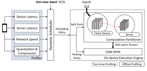
Figure 1. DynO’s system architecture.

As aforementioned, the objective is to overcome the limitations of on-device or cloud execution in targeting heterogeneous devices while adapting to dynamic changes and application SLOs. To this end, we propose DynO (Fig. 1), a framework that addresses these challenges at three levels. First, from an execution perspective, a distributed synergistic approach is introduced with the device and cloud collaborating to run CNN inference. The CNN partitioning is parametrized to tunably assign computations to each end at run time, without modifications to the original model (§ 3.1, 3.2). Second, to minimize the transmission overhead and boost performance, a novel CNN data packing method (CNN-ISPM) is employed that compresses the transferred data beyond what was previously possible and with minimal impact on accuracy (§ 3.3). Finally, to adapt to dynamic changes, a multi-objective scheduler is developed which jointly determines the highest performing partitioning and data packing policy in order to meet the target SLOs (§ 3.4, 3.5).

3.1. Hooking and Instrumentation

To migrate computation between machines and support off-the-shelf models, DynO needs to be able to intercept and even modify CNN operations on-the-fly, transparently to the user. Typically, layers are represented by modules and data as multi-dimensional matrices, called tensors. DynO – implemented on top of PyTorch – intercepts and distributes computation at module (layer) granularity. To achieve this, we implemented a custom hooking framework that targets the PyTorch’s base module class, replacing its call function with our own wrapper function. Fig. 2 shows an example of DynO’s distributed inference. The layer numbers follow the static execution order observed during inference. Overall, DynO’s wrapper function performs the following tasks:
Normal execution: During normal execution, the wrapper invokes the original module function with the original parameters, e.g. blocks 1 – 3 will be executed normally on the client. Furthermore, the wrapper collects runtime information for each executed block (see § 3.4).
Skipped execution: When an operation is assigned to a remote device the original PyTorch module is skipped. As a result, offloaded modules are not executed on the local device, e.g. blocks 4 – 6 will be skipped on the client.
Transfer execution: When computation needs to be transferred, the corresponding dependencies (i.e. tensors) are passed to the data packing queue (§ 3.3), e.g. the output of ops input and 3 will be intercepted as soon as they are computed in order to be transferred to the server. DynO supports multiple transfers of control, in both directions.
Resume execution: When computation is to be resumed on the server, the dependencies are injected from the unpacking queue into the model and execution proceeds normally, e.g. the first dependency is injected before op 4, and the second just before addition.

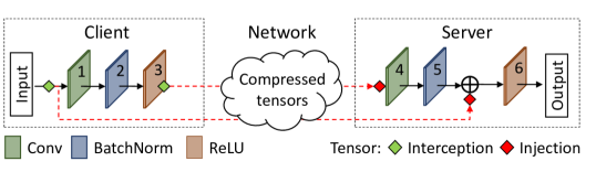
Figure 2. DynO onloading part of a ResNet block.

3.2. Computation Partitioning

DynO can split a CNN in multiple arbitrary partitions and assign those to different devices to run. However, for the cloud onloading scenario, it rarely makes sense to have more than one partition in the real world due to the extra transmission cost which would dominate the overall latency. In essence, packing and transfer are overheads to the inference process, paid only to be later compensated by the faster runtime of the remote end. Once data reside there, we want to run as much as possible on the faster device. This is also evident in Fig. 9, where were DynO to use multiple points, we would pay multiple (un)packings and transfers to hop from the client to server and vice versa. Therefore, we only consider one split point per inference. Once the CNN is partitioned, we run one part on-device and the other on the cloud. This way we initially take advantage of data locality by starting inference on device and, subsequently, find a split point that minimizes the communication overhead if the user’s device is not powerful enough to meet the execution latency requirements.

Internally, DynO captures the CNN workload as a directed acyclic graph (DAG), the dependency graph, with modules as vertices and data dependencies as edges. We deterministically assign a sequence id to the modules of the network based on the the topology of the DAG and the order of execution during the dependency graph construction phase. Finally, when partitioning a CNN with parallel branches, e.g. Inception-v3, or skip connections, e.g. ResNet, the dependencies (edges that cross the cut) have to be transmitted. These dependencies are traced in the offline profiling phase (§ 3.4) for every possible split in a single pass from the dependency graph along with other latency measurements. The selection scheme of the actual split point is detailed in § 3.5. In the example of Fig. 2, the nodes of the graph have already been indexed and the input tensor will be noted as a dependency when partitioning at node 3.

3.3. CNN Communication Optimization

The size of the tensors manipulated by CNN layers can vary greatly, with many reaching several hundreds of KB even for single-input batches. Transferring these tensors can quickly outweigh the benefits of onloading, especially under poor network conditions. To overcome this and optimize the communication between the two processing parties, we introduce an input-specific packing module (CNN-ISPM). The key idea behind CNN-ISPM is the observation that 1) the output tensors of different layers require different degrees of precision for a given level of accuracy, i.e. each layer can have a different bitwidth, and 2) the data representation used at any given point in time needs to accommodate only the tensor values to be transferred to the remote end, i.e. the tensors that constitute dependencies of the selected split point, and further only their values for the specific input at hand. CNN-ISPM employs a CNN-specialized three-phase packing mechanism (Fig. 3) consisting of: input-specific precision quantization (ISQuant), bit shuffling and lossless compression.

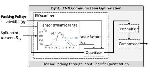
Figure 3. CNN communication optimizer, CNN-ISPM.

Input-Specific Quantization: Precision quantization is frequently used in CNNs to reduce memory footprint and latency (Nikolić et al., 2018). In terms of which data to quantize, most existing schemes target either both weights and activations (Gysel et al., 2018) or only the weights (Zhou et al., 2017) of all layers. In terms of how to quantize, existing works typically adopt linear quantization based on block floating-point (also known as dynamic fixed-point) (Sze et al., 2017; Gysel et al., 2018; Guo et al., 2018; Kouris et al., 2018; Jacob et al., 2018) which dictates a uniform bitwidth and a non-uniform scale factor across the model’s layers. This approach can be expressed as $q_{l}$$=$$\left<b,s_{l}\right>$ for the l-th layer with $b$ the bitwidth and $s_{l}$ the scale factor that determines which bits to keep.

In the majority of existing works, the value of $s_{l}$ is determined at design time by estimating the dynamic range of data over a calibration set (e.g. a subset of the target dataset). This approach is bounded by two main factors. First, a long profiling stage is required in order to determine the scale factors, with the strong assumption that the calibration set is representative of the inference-time data. Second, this approach underutilizes the representational range of the selected bitwidth in cases where the estimated dynamic range does not capture the current input’s range. Fig. 4 illustrates such a case. The symbol $\boldsymbol{D}_{l,i,k}$ denotes the k-th dependency tensor for the i-th input at split point $l$. The estimated dynamic range (grey dotted line) – that has been used at design time to set the scale factor to a fixed value – does not capture the actual range of the input tensor $\boldsymbol{D}_{l,1,k}$.

In contrast to compute- and memory-reducing methods, DynO focuses on optimizing the device-server communication. To this end, a communication-driven quantization method is proposed. DynO’s precision reduction strategy, named ISQuant, entails two key techniques: 1) it applies linear quantization only on the intermediate tensors that have to be transferred between the partitions; and 2) it adapts the scale factor in an input-dependent (sample-specific) manner. As shown in Fig. 4, this approach enables DynO to tightly follow each tensor’s representational needs through an input-adaptive scale factor (e.g. for both $\boldsymbol{D}_{l,1,k}$ and $\boldsymbol{D}_{l,2,k}$). Formally, we express ISQuant as $q_{l,i,k}^{\texttt{ISQuant}}=\left<b_{l},s_{l,i,k}\right>$ with a different bitwidth $b_{l}$ for each layer $l$ and an input-specific (i-th) scale factor $s_{l,i,k}$ for each tensor (k-th) in the split point’s dependencies. In this manner, the scale factor of each tensor is derived at run time to cover the full range of its values (Algorithm 1 lines 2-4). The bitwidth $b_{l}$ constitutes the data packing policy and is dynamically selected by DynO’s scheduler to meet the multi-objective requirements of the target use-case (as detailed in § 3.5).

To demonstrate how ISQuant better captures the dynamic range of the dependency tensors, Fig. 5 shows a comparison of the real and estimated dynamic range for Inception-v3 on ImageNet. For the fixed scale-factor baseline, we divide the validation set into multiple class-balanced calibration sets containing 5% of the samples (20-fold). For each split point (normalized activation index on the x-axis), the real range boxes represent the distribution of values across all validation set samples. For the estimated range, the boxes indicate the estimates’ distribution across the 20 calibration sets. For conciseness, we show every third split point, with similar findings for the remaining splits.

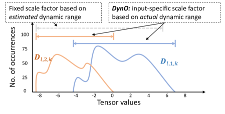
Figure 4. DynO’s input-specific quantization, ISQuant. We depict three dynamic ranges: 1) the start and end points of the blue and orange curves show the actual min and max values for the two input tensors ($\boldsymbol{D}_{l,1,k}$ and $\boldsymbol{D}_{l,2,k}$, respectively), 2) the estimated dynamic range when using fixed, offline estimation (grey dotted line), and 3) the dynamic range captured by DynO for samples $\boldsymbol{D}_{l,1,k}$ and $\boldsymbol{D}_{l,2,k}$ shown as blue and orange solid lines, respectively.

Based on the figure, we make two key observations. First, there is significant variability in the range estimates across different calibration sets. In this respect, the effectiveness of the baseline relies on the faithfulness of the calibration set with regards to the actual processed data upon deployment. Hence, the selection of the calibration set plays a key role in accurately estimating the dynamic range. Second, we observe a large variation in the tensor values. Across all split points, there is a significant amount of outliers that are not captured by the estimated range (e.g. for the 2nd split point, the 2nd quartile is outside the estimated range and multiple points exceed it by much). As a result, all values that lie above the estimated range (45.35% of the samples in Fig. 5) are clamped and numerical error is induced. In contrast to these, the input-specific approach of ISQuant uses the real range of the data to better capture their values when quantizing, thus minimizing the reconstruction error.

Overall, our quantization scheme maximizes the utilization of the selected bitwidth in a per-input sample basis and isolates the approximation to the split-point dependency tensors. Both of these characteristics enable DynO to push the data representation to lower precisions and significantly minimize the data transfer cost. Moreover, while most existing works (Han et al., 2016a; Gysel et al., 2018; Georgiadis, 2019) employ a post-quantization retraining step in order to minimize any induced accuracy losses, our approach – that maintains the rest of the CNN in full precision – enables us to skip the costly retraining step and requires no availability of the training data. As shown in § 4.2.2, ISQuant can lead down to 4 and 5 bits of precision, in most cases, with very low impact on the overall model accuracy.
Bit shuffling: This step transposes the transferred data matrix, so that all least significant bits lie in the same row (Masui et al., 2015). This rearrangement allows the elimination of the compute-heavy Huffman coding (as in GZip) in favor of a faster LZ77-class compressor, such as LZ4.
Compression: To further exploit the redundancy of the transferred data, CNN-ISPM introduces a lossless compression stage. Internally, this stage employs LZ4, a fast lossless compression algorithm. The precedence of ISQuant and bit shuffling results in a significant reduction in the data entropy. In this manner, the resulting sizes are up to 60$\times$ smaller than the original tensors (§ 4.2.1). In § 4.2.1, we present a comparative evaluation of different compressors, justifying the selection of LZ4.
Implementation. Prior to transmitting the tensor dependencies, the client follows the pipeline depicted in Fig. 3 and Algorithm 1. For CNN-ISPM not to starve the client’s resources, we apply the following optimizations. ISQuant is mapped to the client’s mobile GPU (if available), with the min/max operations (lines 2-3) vectorized, and the quantization of each element of tensor $\boldsymbol{D}_{l,i,k}$ performed in parallel (lines 5-7). The bit shuffling and compression phases (lines 9-10) are mapped to the CPU utilizing the SIMD instructions of the target processor (e.g. NEON on ARM cores). Overall, CNN-ISPM is run as a separate thread enabling the pipelining of inference and packing. On the server side, the received data are first decompressed and then dequantized back to the original bitwidth, before being injected to the model to resume the inference computation. We note that this approach has very little impact on the memory consumption compared to local execution, as DynO compresses only the activations that need to be transferred. As such, the memory requirements for the model and the intermediate results are not affected.

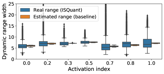
Figure 5. Distribution of estimated range (5% calibration set) vs the real observed range
for Inception-v3 on ImageNet.

With CNN-ISPM, the amount of packing is configurable. If the network conditions are sufficiently good to support the application’s deadlines, higher bitwidths can be used to maximize accuracy. As the network conditions degrade, DynO’s scheduler may choose a more aggressive packing policy by quantizing down to smaller bitwidths. The bitwidth selection process will be described in § 3.5.

Input: Selected split point $l$ and bitwidth $b_{l}$ (packing policy)

         k-th dependency tensor $\boldsymbol{D}_{l,i,k}$ for the i-th input at split point $l$

1

Output: k-th packed tensor to be transferred $\boldsymbol{D}_{l,i,k}^{\text{packed}}$

2

3/* - - - Phase 1 - Input-Specific Quantization - - - */

4 $val_{\text{min}}\leftarrow\min(\boldsymbol{D}_{l,i,k})$

5 $val_{\text{max}}\leftarrow\max(\boldsymbol{D}_{l,i,k})$                             $\left.\begin{array}[]{@{}c@{}}\\ {}\hfil\\ {}\hfil\\ {}\hfil\end{array}\color[rgb]{0,0,0}\right\}\color[rgb]{0,0,0}\begin{tabular}[]{l}Calculate\\ input-dependent\\ scale factor\\ \end{tabular}$

6 $s_{l,i,k}\leftarrow\log_{2}\left(\frac{2^{b_{l}}-1}{val_{\text{max}}-val_{\text{min}}}\right)$

7

8for $d$ in $\boldsymbol{D}_{l,i,k}$ do // loop over the data of the k-th dependency tensor

9      

10      $d^{\text{quant}}\leftarrow(d-val_{\text{min}})\cdot 2^{s_{l,i,k}}$

11 end for

12$\boldsymbol{D}_{l,i,k}^{\text{quant}}\leftarrow[\forall d^{\text{quant}}$]

13

14$\boldsymbol{D}_{l,i,k}^{\text{bitshuffled}}\leftarrow\text{BitShuffle}(\boldsymbol{D}_{l,i,k}^{\text{quant}})$ /* - - Phase 2 - Bit Shuffling - - */

15

16$\boldsymbol{D}_{l,i,k}^{\text{packed}}\leftarrow\text{Compress}(\boldsymbol{D}_{l,i,k}^{\text{bitshuffled}})$ /* - Phase 3 - Compression - */

Algorithm 1 CNN-ISPM’s communication optimization

3.4. Dynamic Profiler

After identifying the dependencies for each possible split point $s$, DynO needs to make decisions about where to split the CNN and how much packing $c$ to apply on the transferred dependencies. These decisions greatly affect the inference i) latency, ii) throughput, iii) accuracy and iv) cost of operation at both ends. DynO makes these decisions by estimating the device, network and server times, as well as the expected accuracy, for each possible configuration $\left<s,c\right>$. The Profiler (Fig. 1) tracks these key performance metrics at two separate phases: i) Offline and ii) Run-time.
Offline profiling: Before deploying a CNN to a set of devices, an initial calibration round is performed to initialize the profiling metrics. First, we note that the size of the data dependencies $d_{\left<s,c\right>}$ and the accuracy loss $Acc_{\left<s,c\right>}$ are not device-dependent. Therefore, these can be profiled once for a given model. In our implementation, the profiler calculates these values using the target task’s validation set. Upon deployment, the profiler estimates the CNN computation times that are device-dependent. This is accomplished by going through a calibration set once, for each available processing unit (e.g. CPU, GPU, NPU) measuring the average time to execute each layer (input-independent) and to compress their dependencies (input-dependent). These are treated as initial values, to be later updated at run time.
Run-time profiling: At run time, the profiler keeps updating the estimated latencies by taking into account the device load and the networking conditions. To estimate the real-world computation latency, the profiler logs the processing unit and memory utilization just before an inference is performed. During inference, DynO records the compute times up to split point $s$ and calculates a scaling factor $SF=\frac{T_{\text{real}\left<s\right>}}{T_{\text{offline}}\left<s\right>}$ between the measured time and the offline estimate. Next, the profiler interprets the scaling factor as a proxy of the device load and uses it to estimate the runtime all other possible splits, e.g. $SF\cdot T^{\text{offline}}_{\left<s^{\prime}\right>}$ for new split $s^{\prime}$.

To estimate the network transfer time, DynO’s profiler monitors the device’s network bandwidth ($B$) and latency ($L$). The transfer time is $L$$+$$\frac{d_{\left<s,c\right>}}{B}$ where $d_{\left<s,c\right>}$ is the data size to be transferred given split $s$ and packing $c$. As networking fluctuates, two moving averages are maintained: a real-time estimate and a historical moving average, $\left<L^{\{\text{rt},h\}},B^{\{\text{rt},h\}}\right>$. Real-time estimates are obtained only if there are transfers in the last 5 minutes. If no such information exists, the historical averages for the same network type are used.

3.5. Dynamic Scheduler

Given the output of the profiler, the dynamic scheduler is responsible for deciding how to distribute the CNN computation and tune the data packing so as to satisfy the application requirements. The dynamic aspect is particularly important for mobile devices where connectivity and load conditions can frequently change (e.g. move from WiFi to 3G). To capture diverse tasks, the scheduler allows developers to define a combination of hard constraints (e.g. inference latency $\leq$ 100 ms) and soft optimization targets (e.g. minimize cloud costs) on a set of metrics. In our current implementation, the set of metrics includes $\mathcal{M}$$=$$\left<\right.$latency, throughput, server cost, device cost, accuracy$\left.\right>$. In DynO, we interpret server (cloud) and device cost as the execution time on the respective side. This formulation can cover a wide range of use-cases. For example, in latency-bound tasks (Yao et al., 2017; Kouris and Bouganis, 2018; Kukkala et al., 2018), one might want to onload as much as possible to the client as long as the inference latency is below a threshold $thr_{\text{lat}}$.

Formally, we capture a hard constraint as $C=\left<m,op,thr\right>$ where $m$$\in$$\mathcal{M}$ is a metric, $op$ is an operator, e.g. $\leq$, and $thr$ is a given threshold value. Similarly, we define a soft optimization target as $O=\left<m,min||max||val\right>$ where a given metric is either maximized, minimized or close to a given value. To capture the importance of each metric, we adopt a multi-objective formulation, where the user supplies a list of prioritized hard constraints $\left<C_{1},...,C_{n}\right>$ and a list of ordered soft optimization targets $\left<O_{1},...,O_{|\mathcal{M}|}\right>$.

Algorithm 2 describes the operation of the scheduler. First, the scheduler uses the estimated network conditions, and device and server loads to update the profiler parameters (line 1). Given the list of prioritized hard constraints, the scheduler iteratively eliminates all (split, packing) configurations $\small\left<s,c\right>$ that violate the constraints in that order (lines 3-6). If at any point no configuration satisfies the constraints, the closest configuration is immediately returned (i.e. fall back to best-effort). If more than one configuration satisfy the constraints, the soft targets are used to sort them (line 7). Finally, the best configuration is returned by the scheduler, with split $s^{*}$ and packing policy $c^{*}$ used to configure the partitioner and CNN-ISPM.

Input: Space of candidate configurations $\Sigma$

         Prioritised hard constraints $\left<C_{1},C_{2},...,C_{n}\right>$

         Prioritised soft targets $\left<O_{1},O_{2},...,O_{|\mathcal{M}|}\right>$

         Current network conditions $net=\left<L,B\right>$

         Current device and server loads $l^{\{\text{dev},\text{server}\}}$

         Profiler data $prf$

Output: Selected configuration $\left<s^{*},c^{*}\right>$

1

2$prf\leftarrow$ UpdateTimings($prf$, $net$, $l^{\text{dev}}$, $l^{\text{server}}$)

3

4$\Sigma^{\text{feasible}}\leftarrow\Sigma$

5 foreach $C_{i}\in\left<C_{1},C_{2},...,C_{n}\right>$ do // discard infeasible configuration

6       $\Sigma^{\text{feasible}}\leftarrow$ DiscardInfeasibleConfigs($prf$, $C_{i}$, $\Sigma^{\text{feasible}}$)

7      

$\Lsh$

VecCheckCond($prf$, $\Sigma^{\text{feasible}}$(:,$M_{i}$), $op_{i}$, $thr_{i}$) $~{}\forall i\in[1,n]$

8      

9 end foreach

10

11$\left<s^{*},c^{*}\right>\leftarrow$ OptUserSoftTargets($prf$, $\left<O_{1},O_{2},...,O_{|\mathcal{M}|}\right>$, $\Sigma^{\text{feasible}}$)

12

$\boldsymbol{\Lsh}$

VecMax/Min($prf$, $\Sigma^{\text{feasible}}$(:,$M_{i}$), $op_{i}$) $~{}\forall i\in[1,|\mathcal{M}|]$

Algorithm 2 Operation of dynamic scheduler upon invocation

Implementation. The scheduler is deployed on the client where the data reside and the inference is initiated. To minimize resource usage, we vectorize the comparison and max/min operations (lines 4-5, 7-8) to utilize SIMD instructions. This way, the scheduler executes in max 14 ms (11 ms geo. mean across examined CNNs on ImageNet) on Jetson’s CPU with a few KB of memory usage (setup details in § 4.1). Finally, the scheduler’s overhead is amortized over multiple inferences as the scheduler is only re-invoked when the profiler metrics change by more than $5\%$.

Pipelining. To further optimize DynO’s throughput under normal server load without backpressure, we apply pipelining. In this respect, the compression, network and inference stages run as separate parallel threads. When the scheduler is instructed to maximize inference throughput, it aims to minimize the maximum latency across these stages, to balance the client, server and network times.

4. Evaluation

4.1. Experimental Setup

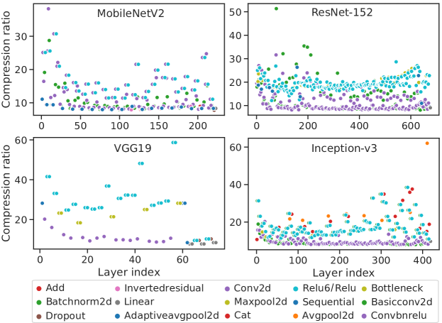
Figure 6. Compression ratio for each model’s layers with CNN-ISPM (using 4 bits).
Colors represent different layer types.

In our experiments, we use a high-end desktop as the server and Jetson Xavier AGX as the client, both connected over Gigabit Ethernet (details are provided at Table 2).

Table 2. Target Platforms

Platform	Processor	Memory	GPU
Server-Desktop	Intel i7-7820X	128GB DDR4	Nvidia GTX1080Ti
Client-Jetson Xavier	8-core ARM-Karmel v8.2	16GB LPDDR4x	512-core Volta

We specifically chose Jetson as our device due to its compact form factor, versatility and adjustable power consumption and computational performance, which makes it ideal for diverse use-cases. To emulate devices of different capabilities, we adjust the TDP and clock rate of the CPU and GPU cores and test against three different power profiles: 1) 30W, using AGX’s MAXN mode (e.g. for drones and robots), 2) 10W (e.g. for smart cameras), 3) underclocked 10W (e.g. smartphones and tablets). To better control network conditions, we simulate them using the average bandwidth and latency across national carriers (Ofcom, 2014) for 3G and 4G networks. For local-area connections (Gb Ethernet 802.3, WiFi-5 802.11ac), we use the nominal speeds of the respective protocol.
Choice of neural networks: We developed DynO on top of PyTorch (1.1.0) and experimented with four ImageNet-pretrained models from torchvision (0.3.0): Inception-v3 (Szegedy et al., 2017), ResNet-152 (He et al., 2016), VGG19 (Simonyan and Zisserman, 2015) and MobileNetV2 (Sandler et al., 2018). Across all experiments, we use a batch size of 1. With respect to input size, Inception-v3 receives $3$$\times$$299$$\times$$299$, while the other three models receive $3$$\times$$224$$\times$$224$. These models represent a diverse range of CNNs with distinct architectures and sizes, from MobileNetV2 with 0.33 GFLOPs and 3.5M parameters, to VGG19 with 20.2 GFLOPs and 143M parameters. Despite the significant progress in model compression and efficient CNN design, existing efforts have focused on a few popular datasets and tasks. In real-world scenarios, where proprietary datasets and complex tasks are targeted, deriving an efficient model without penalizing the accuracy is often not possible. Hence, system designers tend to end up with resource-efficient, but less accurate CNNs. As such, with the exception of MobileNetV2, we intentionally focus on larger networks, where server-assisted execution is more valuable, since these generally offer higher and previously unattainable accuracies on embedded devices. Moreover, ML-powered app developers are reported to deploy DNN models which can be found readily pretrained, rather than architectures at the bleeding edge of deep learning research (Almeida et al., 2021). As such, we include the widely available VGG network in our experiment, despite the fact that it is not anymore in the latency-accuracy Pareto frontier.

4.2. Compression Analysis

We study two main aspects of the packing module, CNN-ISPM: i) which layers are good candidates for compression and how much and how fast they can be compressed; and ii) what is the precision limit we can reach with minimal degradation of the task’s accuracy.

4.2.1. Compression ratio

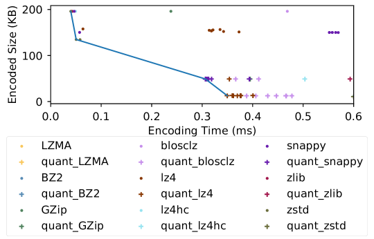
Figure 7. Time vs size of encoding 200KB ReLU activations, without and with 4-bit ISQuant (denoted with the ‘quant’ prefix). Blue line indicates the pareto front of the best size/time tuples.

We started our experiments with two assumptions: i) the widely used ReLU (Nair and Hinton, 2010) activations zero out negative values and thus tend to have high sparsity (Rhu et al., 2018); ii) highly sparse data tend to be highly compressible. To select the best compression scheme, we evaluated the compression ratio and latency of multiple compression schemes when compressing ReLU activations, with and without 4-bit ISQuant. Fig. 7 presents the obtained results when compressing a mid-sized ReLU layer of ResNet-18 over 100 inferences. Lossless compression alone can already provide a 30% reduction with less than 0.1 ms encoding time. Nonetheless, with additional 4-bit quantization we witness an increase in the compression ratio, with up to 95% reduction in size. These results indicate that the ISQuant and LZ4 combination is the best performing, reducing $200KB$ activations by up to 95% in under $0.32$ ms and thus use it for the remaining experiments.

To validate our assumption that ReLUs are indeed within the most compressible components of CNNs, we collected the output tensors of every layer in our evaluated networks and applied CNN-ISPM (Fig. 6). ReLU outputs, spread across the depth of the CNN, consistently yield among the highest compression ratios, reaching up to 60$\times$ for VGG19. The trend is similar for the MobileNetV2 and Inception blocks, ending in one or multiple ReLUs.

Takeaways: Activations such as ReLU are widely spread across popular CNNs and their outputs are prominent candidates for compression, delivering significant size reduction with minimal overhead when using input-specific quantization, bit shuffling and LZ4.

4.2.2. Accuracy sensitivity to compression

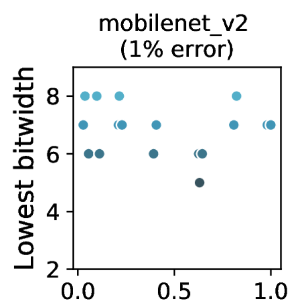
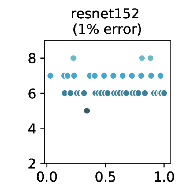
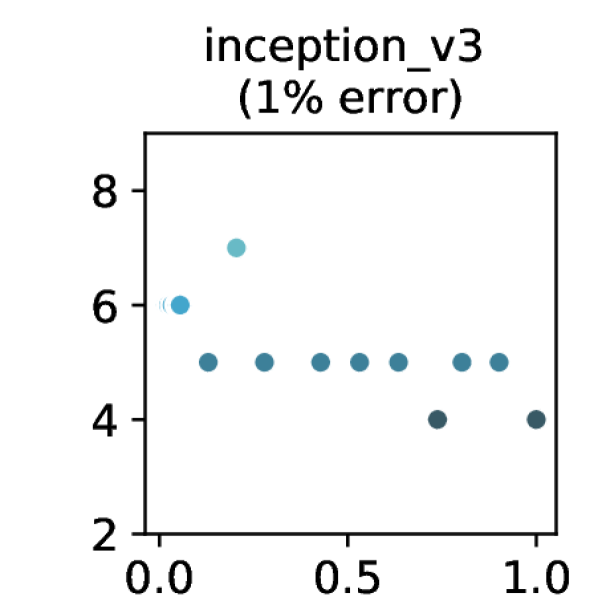
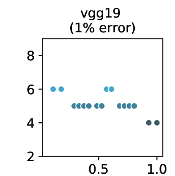
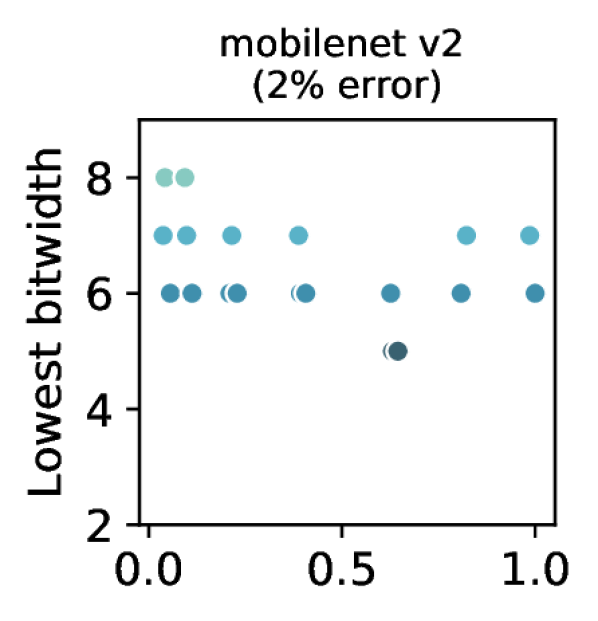
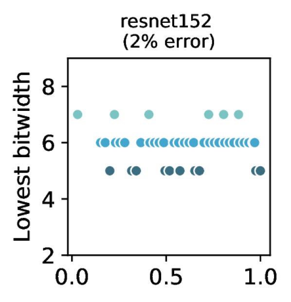
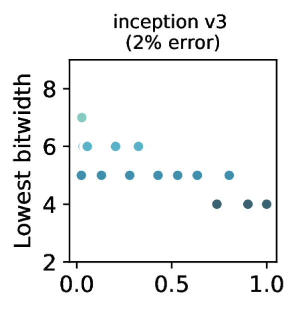
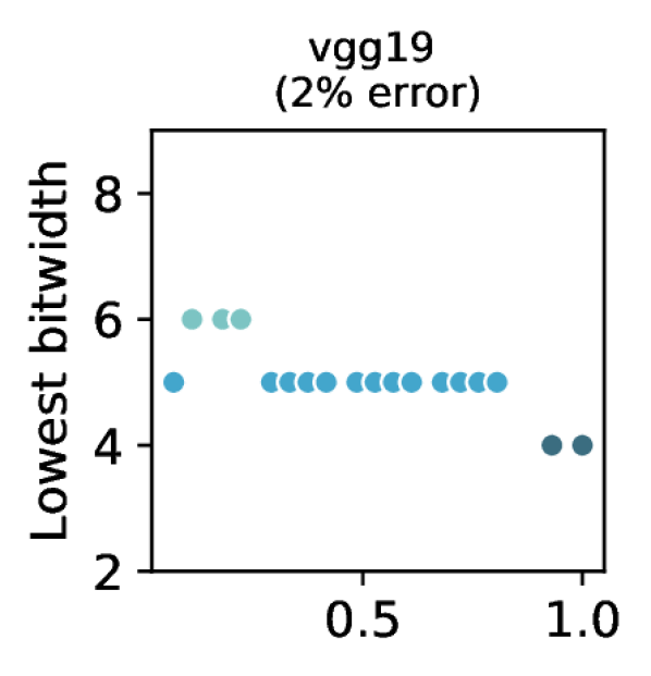
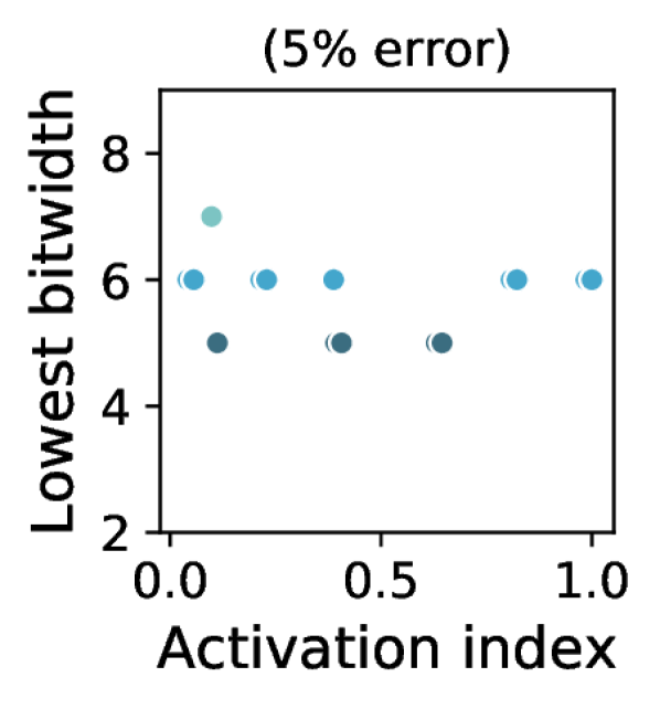
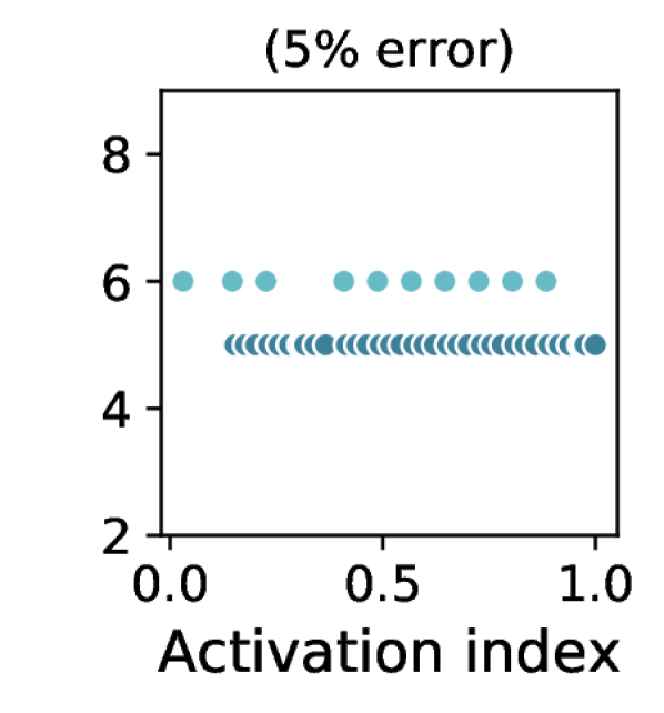
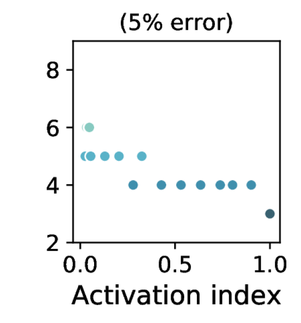
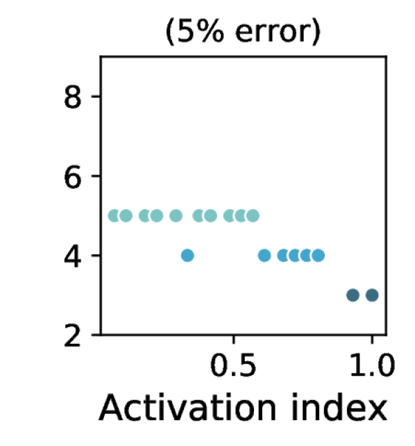
Figure 8. Best ISQuant bitwidth per layer with a max of 1, 2 and 5 pp accuracy drop. Layer indexes are normalized by the number of layers of each CNN. Most CNNs can be quantized to 3-8 bits with minimal accuracy drop.

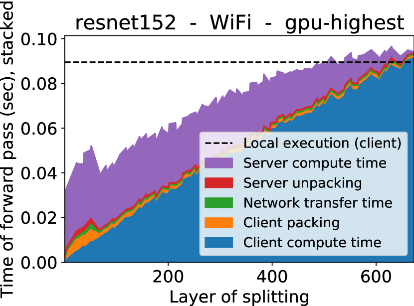
(a) ResNet-152, GPU - WiFi

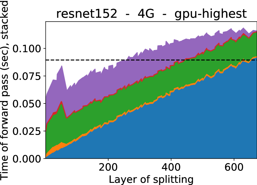
(b) ResNet-152, GPU - 4G.

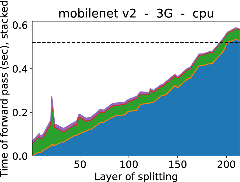
(c) MobileNetV2, CPU - 3G

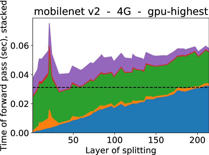
(d) MobileNetV2, GPU - 4G

Figure 9. Breakdown of the runtime and overheads for splitting a CNN at various layers for four very diverse scenarios. For both gpu-highest and cpu, we use the AGX’s MAXN mode.

In addition to the potential space savings of packing, DynO requires estimates of its impact on accuracy to better partition and schedule execution. To achieve this, we apply CNN-ISPM to the dependencies of each possible split and measure the impact on ImageNet’s validation accuracy. Since DynO technically allows partitioning the graph at any layer, this process can become time consuming for larger networks. Driven by our previous results, we reduce the partition search space to layers that only have ReLU dependencies. On average, this heuristic reduces the search space by 81% across the examined CNNs, greatly diminishing both the offline profiling and scheduler runtime. Our packing algorithm is still applicable to other activations, but yields different compression dynamics. The Swish function, for example, would show gains from the smaller range of values towards $-\infty$ instead of ReLU’s hard zero bound.

Fig. 8 shows the lowest bitwidth achievable by ISQuant for an accuracy degradation of $1$, 2 and $5$ percentage points (pp). Rows represent levels of degradation allowance and columns different CNNs. As it can be observed, layers’ resilience to quantization varies from 3 to 8 bits across networks. For Inception-v3 and VGG19, we also observe higher tolerance to quantization deeper in the CNN. Compared to the status-quo 32-bit floats and typical 8-bit quantized precision, we are able to achieve 4-10.6$\times$ and 1-2.6$\times$ smaller size respectively with quantization only. Combining 4-bit ISQuant with the three-staged CNN-ISPM packing mechanism can achieve up to 60$\times$ compression. A 5-pp drop can go as low as 3 bits. Even for critical applications that cannot tolerate drops above 1 pp, there are still many activations that can be quantized down to 5-6 bits, with only three layers needing higher precision across all CNNs.

Takeaways: Different layers have different precision requirements for the same accuracy drop allowance. Split points with ReLUs as dependencies are good candidates, able to be quantized down to 4 bits with under 1-pp accuracy drop. This is important as transfer time is a major deterrent when shipping computation to a remote end which generic offloading systems do not explicitly optimize.

4.3. Performance Analysis

This section assesses the quality of DynO’s $\left<\text{split},\text{packing}\right>$ decisions and the achieved performance on diverse CNNs in a broad range of device capabilities and network conditions.

4.3.1. Split decisions and computation time

Fig. 9 breaks down the DynO’s runtime for four diverse scenarios. For each possible split point (x-axis), we used DynO to run each CNN with the corresponding splitting and measured the runtime breakdown (y-axis). Furthermore, for each split point we configured CNN-ISPM with the shortest bitwidth that led to less than 1-pp drop in accuracy.

In Fig. 9(a), a large-scale CNN (ResNet-152) is run on a powerful client GPU (30W Jetson) under good network conditions (WiFi). Despite the powerful client, the fast, reliable channel results in remote execution yielding lower latency, due to the low transfer time. The partition point of zero signifies the server-only execution, while the device-only execution is explicitly shown by the horizontal dashed line. For all partition points in between (35-90 ms), there are savings in cloud usage, by progressively pushing more computation towards the device’s spare resources.

Fig. 9(b) shows the same scenario over 4G. The significantly higher transmission overhead in 4G makes remote execution less favorable, especially after the device executes the first 250 layers. Moreover, we can see that there is a bigger impact from layers producing more information. Nonetheless, we note that remote execution would be unfeasible without CNN-ISPM and highlight that, for both Fig. 9(a) and 9(b), when the server and client times are balanced (e.g. layer 150 in Fig. 9(a)), DynO can double the throughput through pipelining.

Fig. 9(c) depicts a different scenario that represents most mid-tier smartphones, where inference runs on CPUs. To realistically capture this scenario, we ran a lightweight CNN (MobileNetV2). Despite the mobile-friendly CNN and even when 3G is used, the remote assistance is almost always a better option. In contrast, when a more powerful compute engine is employed (GPU in Fig. 9(d)), the faster local inference time can lead DynO’s scheduler to perform full onloading and execute locally. Across all cases, the overhead of CNN-ISPM (“client packing” in Fig. 9) is relatively small compared to the total CNN computation times.

Takeaways: The target CNN’s workload, the client/server capabilities and the network conditions can result in different execution dynamics. For most settings, there are opportunities to onload computation to the client to optimize for cloud costs, throughput or latency. This also demonstrates why a dynamic scheduler can play a key role in coping with such dynamic and heterogeneous environments.

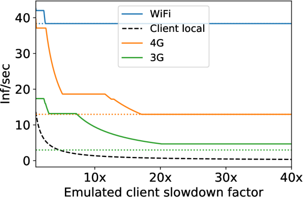
(a) ResNet-152

(b) MobileNetV2

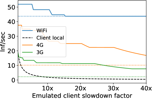
(c) Inception-v3

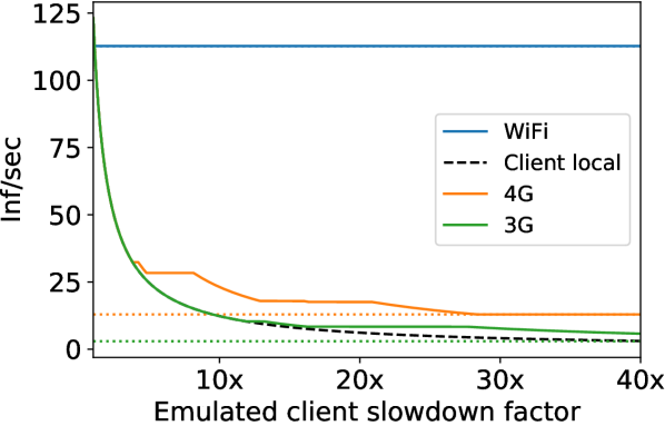
(d) VGG19

Figure 10. Throughput achieved for varying network conditions and device capabilities/load. Dotted lines represent full-server execution (using CNN-ISPM on the CNN’s inputs). Dashed black lines represent local-only execution. For reference, flagship mobile GPUs/CPUs are typically 5$\times$/20$\times$ slower than Jetson’s GPU, respectively, while low-tier devices around 35$\times$ slower.

4.3.2. DynO inference throughput

In this section, we assess DynO’s attainable performance in throughput-driven cases. To this end, we configured DynO to use pipelining and its scheduler to maximize inference throughput with an accuracy drop tolerance of $\leq 1$ pp. In Fig. 10, we scale the client CNN computation and packing times by a given factor as a proxy of different client capabilities. Different slowdown factors along the x-axis can also be interpreted as fluctuating on-device load.

For all CNNs, splitting the network can result in significant throughput gains compared to full-remote execution. For ResNet-152 (Fig. 10(a)), DynO always yields at least equal or higher throughput compared to both fully-local and remote executions. For smaller CNNs such as MobileNetV2 (Fig. 10(b)), DynO achieves significant speedups of up to 10.5$\times$ and 35.5$\times$ over full-server and client execution, respectively. On the other hand, VGG19 (Fig. 10(d)) is a notable example of a CNN with significant transmission overhead due to its large tensor sizes, especially under cellular networks. For such CNNs the scheduler defaults to local execution, even for devices that are 5$\times$ slower than Jetson. Nonetheless, when targeting even more resource-constrained devices ($>5\times$), DynO outperforms local execution by up to 4.2$\times$ for 4G and 1.8$\times$ for 3G.

Overall, for faster devices (i.e. left of the x-axis in Fig. 10(a)-10(d)), DynO adopts a more strict onloading policy by assigning more workload to the client. As the device becomes busier (e.g. increased load from concurrent apps) or a lower-end platform is targeted (to the right of the x-axis), DynO applies onloading more conservatively and the computation is progressively assisted by the server.

Takeaways: In most cases, it is possible to find a split where pipelining improves throughput, with significant gains over local and remote execution. In general, the faster the client, the more justified it is to onload computation there. Only in scenarios with very slow network, huge CNNs or low-end clients, does the behavior default to one of the two extremes. These diverse decisions observed under varying device conditions highlight the need for joint decisions on the onloading and transmission policies at runtime.

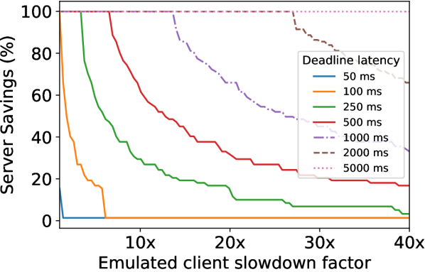
(a) ResNet-152 - WiFi

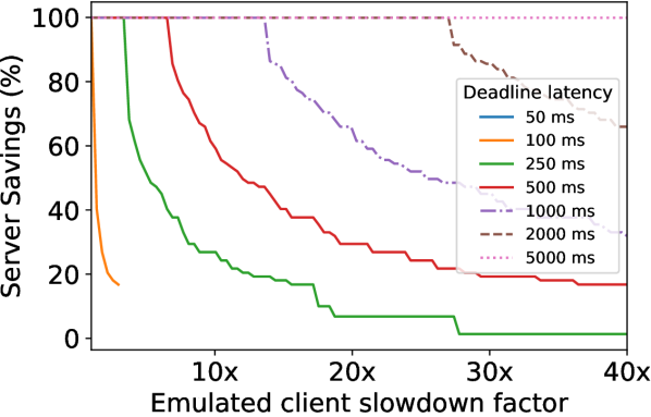
(b) ResNet-152 - 4G

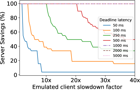
(c) MobileNetV2 - WiFi

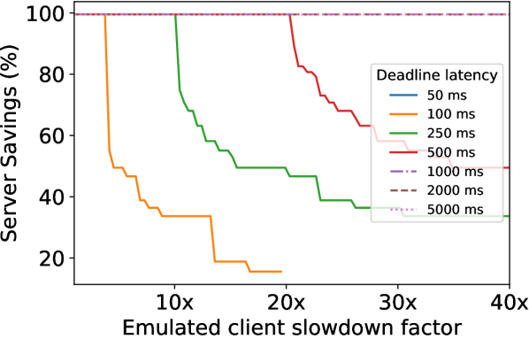
(d) MobileNetV2 - 4G

Figure 11. Percentage of server computation saved for varying device capabilities to meet a latency deadline. When a line stops (e.g. (b) 100 ms latency), the requested deadline cannot be met.

4.3.3. DynO server savings vs. performance SLOs

Here, we assess DynO’s multi-objective scheduler’s ability to capture novel complex scenarios such as saving cloud cost under strict performance constraints and diverse network conditions. Fig. 11 shows the attainable server savings when a certain latency deadline is requested. For ResNet-152 (Fig. 11(a)-11(b)), DynO onloads the whole computation when the deadlines are lenient ($>$2s per inference) even for slower clients (27$\times$ slower than 30W Jetson). For tighter latency deadlines, server assistance is required. However, across all deadline goals DynO can gradually onload computation based on the device capabilities, saving cloud costs. For instance, for a 500-ms deadline in Fig. 11(a), DynO onloads the whole network for high-tier devices, and close to 20% for low-tier devices. Similar flexibility is shown over 4G (Fig. 11(b)), although stricter deadlines of 50 ms and 100 ms cannot always be met for slower devices. Lighter networks such as MobileNetV2 (Fig. 11(c)-11(d)) show similar performance, but achieve higher server savings as a larger part can be executed on-device.

Takeaways: Given the heterogeneous device landscape, we can automatically optimize how much is onloaded to each device, based on the CNN, device capabilities and load, as well as network conditions, resulting in significant savings and improved inference performance.

4.3.4. Comparison with existing frameworks

In this section, we evaluate DynO against the state-of-the-art CNN offloading system, Neurosurgeon (Section 2), and the status-quo server- and device-only baselines. For the server-only baseline, we employed an optimized variant that is enhanced with CNN-ISPM’s compression to pack the inputs prior to transmission. DynO’s scheduler was configured to maximize throughput with an 1-pp of maximum accuracy drop tolerance. Similarly, Neurosurgeon was implemented with latency minimization as its objective. Fig. 12 shows the achieved throughput for varying network conditions and devices. We can see that server-only execution is communication-bound, with its throughput following the trajectory of the available bandwidth. In contrast, Neurosurgeon can tunably distribute computation between device and server. However, its scheduler provides polarized partitioning, switching from “offload-nothing” to “offload-everything”. The gradual performance increase deceptively resembles progressive offloading, but depicts in fact the increase of bandwidth when Neurosurgeon selects full-offloading. Compared to the enhanced server-only baseline, Neurosurgeon has a lower peak throughput due to CNN-ISPM’s compression that the former incorporates.

DynO’s achieves the highest throughput across all setups. First, we observe that for powerful devices (Jetson-30W in Fig. 12(a)-12(b)) and lower network speeds ($<$1Mbps), distributed execution cannot surpass the throughput of client-only execution and hence DynO selects on-device execution. This manifests because the cost of packing and transferring the data outweighs the benefits of server assistance. On the other hand, for lower-end devices (e.g. Fig. 12(c)-12(d)), distributed execution yields speedups even under scarce network conditions. As networking improves (to the right of Fig. 12(c)), DynO’s pipelining provides a further boost with up to $10\times$ higher throughput than local execution at 10Mbps, before its scheduler switches to full offloading. Finally, DynO yields equal or higher peak inference rate than the “full-server” paradigm, attributed to the smaller transfer size due to the additional ISQuant step of CNN-ISPM as well as the strategic adaptive selection of split point.

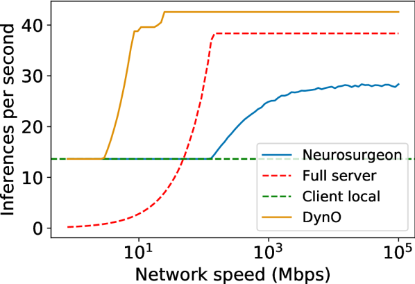
(a) ResNet-152 GPU Client

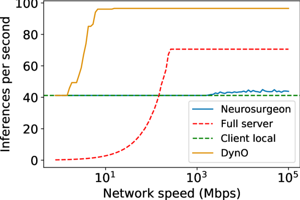
(b) MobileNetV2 GPU Client

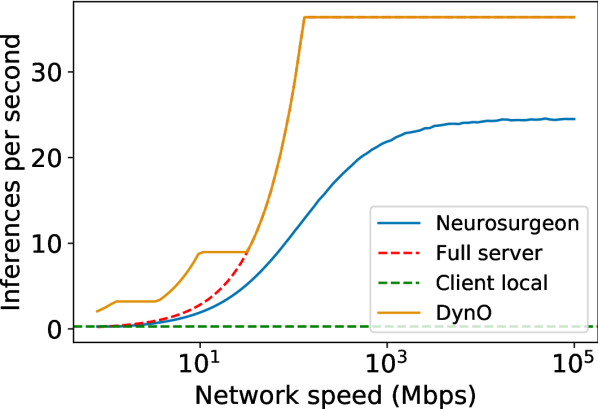
(c) ResNet-152 CPU Client

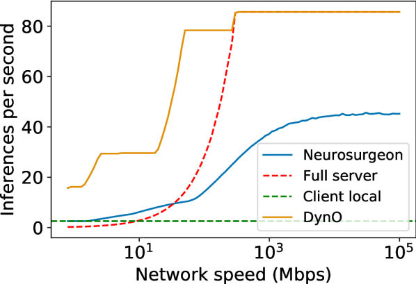
(d) MobileNetV2 CPU Client

Figure 12. Distributed throughput with pipelining.

Compared to Neurosurgeon, DynO consistently delivers higher throughput across all settings. On more compute-capable devices (Fig. 12(a)-12(b)), Neurosurgeon selects device-only execution for a significant portion of bandwidths. This is due to the fast processing of the client and the high communication cost. In contrast, DynO’s CNN-ISPM mechanism significantly reduces the volume of transferred data and effectively alleviates the communication overhead. Hence, while Neurosurgeon requires high bandwidths to switch from on-device execution ($>$20Mbps for ResNet-152 and $>$100Mbps for MobileNetV2), DynO significantly reduces the bandwidth needs and makes distributed execution feasible below 1Mbps. On lower-tier devices (Fig. 12(c)-12(d)), although Neurosurgeon switches to offloading from earlier on due to the slower client, DynO is still able to exploit distributed execution from very low bandwidths and with higher throughput (up to 6.5$\times$) due to the faster packed transmission of dependencies. Moreover, under abundant bandwidth (to the right of the x-axis), the impact of DynO’s pipelining dominates, leading to speedup of up to 7.9$\times$.
Takeaways: The transfer size of dependencies when onloading plays a critical role to the feasible splits of a CNN, especially under bandwidth-constrained channels. As such, the co-optimization of both the selected split point and data packing strategy leads to throughput gains not previously attainable. Moreover, in streaming scenarios, pipelining offers an additional boost in the system’s throughput.

4.4. Energy Consumption

In this experiment, we quantify the energy consumption of DynO’s components in different deployment scenarios compared against the server-only and device-only baselines. Computation energy (CPU, GPU) was measured from the OS probes on Jetson Xavier (underclocked 10W), while the transmission energy was quantified over (Anonymous Provider’s) 4G network with a Huawei E3372 USB adapter connected to a Monsoon AAA10F power monitor. We used the 10-watt mode of Jetson Xavier to better represent the current power-constrained mobile platforms.

Fig. 13 depicts the energy breakdown per component, measured over 100 inferences of Inception-v3. From top to bottom, the first bar represents the case where no onloading occurs, i.e. the client transfers the JPEG compressed data to the server for inference. This yields the highest energy consumption, at 524 mJ per inference, due to the size of the transferred sample. For the next three bars, we vary the SLO – expressed as the percentage of max allowed latency compared to device-only inference – which in turn leads DynO to select different $\left<\text{split},\text{packing}\right>$ parameters. We witness lower overall energy consumption per sample, ranging from 61.8% to 93.6% of the server-only, a fact that we attribute to the significant impact of CNN-ISPM’s packing. Last, the bottom bar depicts the device-only inference, which yields 95% of the server-only energy.
Takeaways: Even without explicitly optimizing for it, there can be energy gains from onloaded execution from the partial on-device computation and compressed transmission.

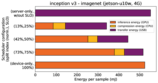
Figure 13. Energy consumption of DynO vs. baselines. SLOs are expressed as
percentages of the device-only latency.

5. Limitations & Future work

While DynO supports a wide range of features and DNN architectures, there are limitations in our study. First, we only consider onloading between two devices and assume models already reside in both ends. Model distribution (Jeong et al., 2018) and client multi-tenancy (Fang et al., 2019) on the server side are interesting adjacent issues, but we do not tackle them in this study.

In terms of our evaluation, we varied the network conditions through traffic shaping to assess our scheduler behavior. Moreover, we did not evaluate on heterogeneous devices, but rather targeted the highly configurable Jetson AGX, which enabled us to use it as a proxy for a wide range of device tiers by performing dynamic voltage and frequency scaling and linearly scaling the measured latency. Last, we focus our paper on widely deployed CNNs which largely employ ReLU activations. Different networks, such as RNNs or models with different activation functions (e.g. Swish (Ramachandran et al., 2018) or PReLUs (He et al., 2015)), could also have compression potential under onloading. Nonetheless, DynO can still be beneficial for more generic, non-sparsity-inducing split points, as shown in Fig. 6.

With respect to MobileNetV2’s execution on Xavier’s CPU, we noticed a bottlenecked execution behaviour with PyTorch and NNPACK on Xavier’s CPU. Results from our profiling with NSight Systems (v. 2021.5) show frequent context switching and underutilisation of cores, even under varying thread counts. This indicates a low computation-to-communication ratio, but would require further investigation.

Furthermore, RNN-based models, such as LSTMs (Hochreiter and Schmidhuber, 1997) and GRUs (Dey and Salem, 2017), constitute a special case when it comes to onloading due to their recurrence property: the RNN’s internal state constitutes an inter-sample dependency that is not present in CNNs. As such, if the state-update computation is moved from the device to the server, or vice versa, the current state also has to be transferred to the other party. Hence, although DynO’s partitioning strategy generalizes across DNN architectures through its automatic identification of split-point dependencies, RNNs would require a dedicated treatment. In the future, we would like to extend our work on different architectures and use-cases, and showcase the generalizability of our proposed framework.

6. Conclusion

This paper presents DynO, a distributed CNN inference framework that seamlessly splits computation across device and cloud. By exploiting the variable precision requirements along a given CNN, the proposed system introduces an input-specific quantization method that tunably minimizes the data transfer overhead. At run time, DynO jointly tunes the splitting and data packing policy to tailor the execution to the use-case multi-objective needs. DynO delivers significant performance gains over state-of-the-art CNN offloading systems, while saving on cloud cost by onloading to the capable clients, without sacrificing energy efficiency.

References

- (1)
- Almeida et al. (2019) Mario Almeida, Stefanos Laskaridis, Ilias Leontiadis, Stylianos I. Venieris, and Nicholas D. Lane. 2019. EmBench: Quantifying Performance Variations of Deep Neural Networks Across Modern Commodity Devices. In 3rd International Workshop on Deep Learning for Mobile Systems and Applications (EMDL). ACM, 1–6.
- Almeida et al. (2021) Mario Almeida, Stefanos Laskaridis, Abhinav Mehrotra, Lukasz Dudziak, Ilias Leontiadis, and Nicholas D. Lane. 2021. Smart at What Cost? Characterising Mobile Deep Neural Networks in the Wild. In Proceedings of the 21st ACM Internet Measurement Conference (Virtual Event) (IMC ’21). Association for Computing Machinery, New York, NY, USA, 658–672. https://doi.org/10.1145/3487552.3487863
- Antonini et al. (2019) Mattia Antonini, Tran Huy Vu, Chulhong Min, Alessandro Montanari, Akhil Mathur, and Fahim Kawsar. 2019. Resource Characterisation of Personal-Scale Sensing Models on Edge Accelerators. In Proceedings of the First International Workshop on Challenges in Artificial Intelligence and Machine Learning for Internet of Things (AIChallengeIoT). ACM, 49–55.
- Blalock et al. (2020) Davis Blalock, Jose Javier Gonzalez Ortiz, Jonathan Frankle, and John Guttag. 2020. What is the State of Neural Network Pruning? In Proceedings of Machine Learning and Systems (MLSys). Vol. 2. 129–146.
- Burgess (2019) J. Burgess. 2019. RTX ON – The NVIDIA TURING GPU. In 2019 IEEE Hot Chips 31 Symposium (HCS). 1–27. https://doi.org/10.1109/HOTCHIPS.2019.8875651
- Cartas et al. (2019) Alejandro Cartas, Martin Kocour, Aravindh Raman, Ilias Leontiadis, Jordi Luque, Nishanth Sastry, Jose Nuñez-Martinez, Diego Perino, and Carlos Segura. 2019. A Reality Check on Inference at Mobile Networks Edge. In Proceedings of the 2nd International Workshop on Edge Systems, Analytics and Networking (EdgeSys). 54–59.
- Chun et al. (2011) Byung-Gon Chun, Sunghwan Ihm, Petros Maniatis, Mayur Naik, and Ashwin Patti. 2011. CloneCloud: Elastic Execution Between Mobile Device and Cloud. In Proceedings of the Sixth Conference on Computer Systems (EuroSys ’11). 301–314.
- Chung et al. (2018) E. Chung et al. 2018. Serving DNNs in Real Time at Datacenter Scale with Project Brainwave. IEEE Micro 38, 2 (2018), 8–20.
- Cuervo et al. (2010) Eduardo Cuervo, Aruna Balasubramanian, Dae-ki Cho, Alec Wolman, Stefan Saroiu, Ranveer Chandra, and Paramvir Bahl. 2010. MAUI: Making Smartphones Last Longer with Code Offload. In International Conference on Mobile Systems, Applications, and Services (MobiSys).
- Dey and Salem (2017) Rahul Dey and Fathi M Salem. 2017. Gate-Variants of Gated Recurrent Unit (GRU) Neural Networks. In 2017 IEEE 60th international midwest symposium on circuits and systems (MWSCAS). IEEE, 1597–1600.
- Fang et al. (2019) Zhou Fang, Jeng-Hau Lin, Mani B. Srivastava, and Rajesh K. Gupta. 2019. Multi-Tenant Mobile Offloading Systems for Real-Time Computer Vision Applications. In Proceedings of the 20th International Conference on Distributed Computing and Networking (ICDCN). 21–30.
- Georgiadis (2019) Georgios Georgiadis. 2019. Accelerating Convolutional Neural Networks via Activation Map Compression. In Proceedings of the IEEE/CVF Conference on Computer Vision and Pattern Recognition (CVPR).
- Gordon et al. (2012) Mark S. Gordon, D. Anoushe Jamshidi, Scott Mahlke, Z. Morley Mao, and Xu Chen. 2012. COMET: Code Offload by Migrating Execution Transparently. In USENIX Conference on Operating Systems Design and Implementation (OSDI).
- Guo et al. (2018) K. Guo, L. Sui, J. Qiu, J. Yu, J. Wang, S. Yao, S. Han, Y. Wang, and H. Yang. 2018. Angel-Eye: A Complete Design Flow for Mapping CNN Onto Embedded FPGA. IEEE Transactions on Computer-Aided Design of Integrated Circuits and Systems (TCAD) 37, 1 (2018), 35–47.
- Gysel et al. (2018) P. Gysel, J. Pimentel, M. Motamedi, and S. Ghiasi. 2018. Ristretto: A Framework for Empirical Study of Resource-Efficient Inference in Convolutional Neural Networks. IEEE Transactions on Neural Networks and Learning Systems (TNNLS) 29, 11 (2018), 5784–5789.
- Han et al. (2016a) Song Han, Huizi Mao, and William J Dally. 2016a. Deep Compression: Compressing Deep Neural Networks with Pruning, Trained Quantization and Huffman Coding. In International Conference on Learning Representations (ICLR).
- Han et al. (2016b) Seungyeop Han, Haichen Shen, Matthai Philipose, Sharad Agarwal, Alec Wolman, and Arvind Krishnamurthy. 2016b. MCDNN: An Approximation-Based Execution Framework for Deep Stream Processing Under Resource Constraints. In Proceedings of the 14th Annual International Conference on Mobile Systems, Applications, and Services (MobiSys).
- Hazelwood et al. (2018) K. Hazelwood, S. Bird, D. Brooks, S. Chintala, U. Diril, D. Dzhulgakov, M. Fawzy, B. Jia, Y. Jia, A. Kalro, J. Law, K. Lee, J. Lu, P. Noordhuis, M. Smelyanskiy, L. Xiong, and X. Wang. 2018. Applied Machine Learning at Facebook: A Datacenter Infrastructure Perspective. In 2018 IEEE International Symposium on High Performance Computer Architecture (HPCA). 620–629.
- He et al. (2015) Kaiming He, Xiangyu Zhang, Shaoqing Ren, and Jian Sun. 2015. Delving Deep into Rectifiers: Surpassing Human-Level Performance on ImageNet Classification. In International Conference on Computer Vision (ICCV). 1026–1034.
- He et al. (2016) K. He, X. Zhang, S. Ren, and J. Sun. 2016. Deep Residual Learning for Image Recognition. In IEEE Conference on Computer Vision and Pattern Recognition (CVPR). 770–778.
- Hochreiter and Schmidhuber (1997) Sepp Hochreiter and Jürgen Schmidhuber. 1997. Long Short-Term Memory. Neural computation 9, 8 (1997), 1735–1780.
- Hu et al. (2019) Chuang Hu, Wei Bao, Dan Wang, and Fengming Liu. 2019. Dynamic Adaptive DNN Surgery for Inference Acceleration on the Edge. Proceedings - IEEE INFOCOM (2019), 1423–1431.
- Huang et al. (2020) Jin Huang, Colin Samplawski, Deepak Ganesan, Benjamin Marlin, Heesung Kwon, and Paper Xxx. 2020. CLIO: Enabling Automatic Compilation of Deep Learning Pipelines across IoT and Cloud. In Proceedings of the 26th Annual International Conference on Mobile Computing and Networking (MobiCom).
- Ignatov et al. (2019) Andrey Ignatov, Radu Timofte, Andrei Kulik, Seungsoo Yang, Ke Wang, Felix Baum, Max Wu, Lirong Xu, and Luc Van Gool. 2019. AI Benchmark: All About Deep Learning on Smartphones in 2019. In ICCV Workshops (ICCVW).
- Jacob et al. (2018) Benoit Jacob, Skirmantas Kligys, Bo Chen, Menglong Zhu, Matthew Tang, Andrew Howard, Hartwig Adam, and Dmitry Kalenichenko. 2018. Quantization and Training of Neural Networks for Efficient Integer-Arithmetic-Only Inference. In Proceedings of the IEEE Conference on Computer Vision and Pattern Recognition (CVPR).
- Jayakodi et al. (2020a) Nitthilan Kanappan Jayakodi, Syrine Belakaria, Aryan Deshwal, and Janardhan Rao Doppa. 2020a. Design and Optimization of Energy-Accuracy Tradeoff Networks for Mobile Platforms via Pretrained Deep Models. ACM Trans. Embed. Comput. Syst. (TECS) 19, 1, Article 4 (2020).
- Jayakodi et al. (2018) Nitthilan Kannappan Jayakodi, Anwesha Chatterjee, Wonje Choi, Janardhan Rao Doppa, and Partha Pratim Pande. 2018. Trading-off Accuracy and Energy of Deep Inference on Embedded Systems: A Co-Design Approach. IEEE Transactions on Computer-Aided Design of Integrated Circuits and Systems (TCAD) 37, 11 (2018), 2881–2893.
- Jayakodi et al. (2020b) Nitthilan Kanappan Jayakodi, Janardhan Rao Doppa, and Partha Pratim Pande. 2020b. SETGAN: Scale and Energy Trade-Off GANs for Image Applications on Mobile Platforms. In Proceedings of the 39th International Conference on Computer-Aided Design (ICCAD). 1–9.
- Jeong et al. (2018) Hyuk-Jin Jeong, Hyeon-Jae Lee, Chang Hyun Shin, and Soo-Mook Moon. 2018. IONN: Incremental Offloading of Neural Network Computations from Mobile Devices to Edge Servers. Proceedings of the ACM Symposium on Cloud Computing (2018), 401–411.
- Jouppi et al. (2017) Norman P. Jouppi et al. 2017. In-Datacenter Performance Analysis of a Tensor Processing Unit. In International Symposium on Computer Architecture (ISCA).
- Kang et al. (2017) Yiping Kang, Johann Hauswald, Cao Gao, Austin Rovinski, Trevor Mudge, Jason Mars, and Lingjia Tang. 2017. Neurosurgeon: Collaborative Intelligence Between the Cloud and Mobile Edge. International Conference on Architectural Support for Programming Languages and Operating Systems (ASPLOS) (2017), 615–629.
- Kouris and Bouganis (2018) A. Kouris and C. Bouganis. 2018. Learning to Fly by MySelf: A Self-Supervised CNN-Based Approach for Autonomous Navigation. In IEEE/RSJ International Conference on Intelligent Robots and Systems (IROS). 1–9.
- Kouris et al. (2018) A. Kouris, S. I. Venieris, and C. Bouganis. 2018. CascadeCNN: Pushing the Performance Limits of Quantisation in Convolutional Neural Networks. In 2018 28th International Conference on Field Programmable Logic and Applications (FPL). 155–1557.
- Kouris et al. (2021) Alexandros Kouris, Stylianos I. Venieris, Stefanos Laskaridis, and Nicholas D. Lane. 2021. Multi-Exit Semantic Segmentation Networks. In arXiv.
- Kukkala et al. (2018) V. K. Kukkala, J. Tunnell, S. Pasricha, and T. Bradley. 2018. Advanced Driver-Assistance Systems: A Path Toward Autonomous Vehicles. IEEE Consumer Electronics Magazine 7, 5 (2018), 18–25.
- Laskaridis et al. (2021) Stefanos Laskaridis, Alexandros Kouris, and Nicholas D. Lane. 2021. Adaptive Inference through Early-Exit Networks: Design, Challenges and Directions. In Proceedings of the 5th International Workshop on Embedded and Mobile Deep Learning (EMDL). 1–6.
- Laskaridis et al. (2020a) Stefanos Laskaridis, Stylianos I. Venieris, Mario Almeida, Ilias Leontiadis, and Nicholas D. Lane. 2020a. SPINN: Synergistic Progressive Inference of Neural Networks over Device and Cloud. In Proceedings of the 26th Annual International Conference on Mobile Computing and Networking (MobiCom).
- Laskaridis et al. (2020b) Stefanos Laskaridis, Stylianos I. Venieris, Hyeji Kim, and Nicholas D. Lane. 2020b. HAPI: Hardware-Aware Progressive Inference. In 2020 IEEE/ACM International Conference On Computer Aided Design (ICCAD). 1–9.
- Lee et al. (2019) Taegyeong Lee, Zhiqi Lin, Saumay Pushp, Caihua Li, Yunxin Liu, Youngki Lee, Fengyuan Xu, Chenren Xu, Lintao Zhang, and Junehwa Song. 2019. Occlumency: Privacy-Preserving Remote Deep-Learning Inference Using SGX. In The 25th Annual International Conference on Mobile Computing and Networking (MobiCom).
- Li et al. (2019b) En Li, Liekang Zeng, Zhi Zhou, and Xu Chen. 2019b. Edge AI: On-Demand Accelerating Deep Neural Network Inference via Edge Computing. IEEE Transactions on Wireless Communications (TWC) 19, 1 (2019), 447–457.
- Li et al. (2019a) Hongshan Li, Chenghao Hu, Jingyan Jiang, Zhi Wang, Yonggang Wen, and Wenwu Zhu. 2019a. JALAD: Joint Accuracy-And Latency-Aware Deep Structure Decoupling for Edge-Cloud Execution. In International Conference on Parallel and Distributed Systems (ICPADS). 671–678.
- Mao et al. (2017a) Jiachen Mao, Xiang Chen, Kent W. Nixon, Christopher Krieger, and Yiran Chen. 2017a. MoDNN: Local distributed mobile computing system for Deep Neural Network. In Design, Automation and Test in Europe (DATE).
- Mao et al. (2017b) Jiachen Mao, Zhongda Yang, Wei Wen, Chunpeng Wu, Linghao Song, Kent W. Nixon, Xiang Chen, Hai Li, and Yiran Chen. 2017b. MeDNN: A distributed mobile system with enhanced partition and deployment for large-scale DNNs. In International Conference on Computer-Aided Design (ICCAD). 751–756.
- Masui et al. (2015) Kiyoshi Masui, Mandana Amiri, Liam Connor, Meiling Deng, Mateus Fandino, Carolin Höfer, Mark Halpern, David Hanna, Adam D Hincks, Gary Hinshaw, et al. 2015. A compression scheme for radio data in high performance computing. Astronomy and Computing 12 (2015), 181–190.
- Mo et al. (2020) Fan Mo, Ali Shahin Shamsabadi, Kleomenis Katevas, Soteris Demetriou, Ilias Leontiadis, Andrea Cavallaro, and Hamed Haddadi. 2020. DarkneTZ: Towards Model Privacy at the Edge Using Trusted Execution Environments. In Proceedings of the 18th International Conference on Mobile Systems, Applications, and Services (MobiSys). 161–174.
- Nair and Hinton (2010) Vinod Nair and Geoffrey E. Hinton. 2010. Rectified Linear Units Improve Restricted Boltzmann Machines. In International Conference on Machine Learning (ICML). 807–814.
- Nikolić et al. (2018) M. Nikolić, M. Mahmoud, and A. Moshovos. 2018. Characterizing Sources of Ineffectual Computations in Deep Learning Networks. In 2018 IEEE International Symposium on Workload Characterization (IISWC). 86–87.
- Ofcom (2014) Ofcom. 2014. 3G and 4G Network Speeds. https://www.ofcom.org.uk/about-ofcom/latest/media/media-releases/2014/3g-4g-bb-speeds.
- Panda et al. (2016) Priyadarshini Panda, Abhronil Sengupta, and Kaushik Roy. 2016. Conditional Deep Learning for Energy-Efficient and Enhanced Pattern Recognition. In 2016 Design, Automation & Test in Europe Conference & Exhibition (DATE). IEEE, 475–480.
- PyTorch (2021) PyTorch. 2021. Dynamic Quantization. https://pytorch.org/tutorials/recipes/recipes/dynamic_quantization.html. [Retrieved: ].
- Ramachandran et al. (2018) Prajit Ramachandran, Barret Zoph, and Quoc V Le. 2018. Searching for Activation Functions. In International Conference on Learning Representations (ICLR) workshops.
- Rhu et al. (2018) M. Rhu, M. O’Connor, N. Chatterjee, J. Pool, Y. Kwon, and S. W. Keckler. 2018. Compressing DMA Engine: Leveraging Activation Sparsity for Training Deep Neural Networks. In International Symposium on High Performance Computer Architecture (HPCA). 78–91.
- Ryan (2011) Mark D. Ryan. 2011. Cloud Computing Privacy Concerns on Our Doorstep. Commun. ACM 54, 1 (2011), 36–38.
- Sandler et al. (2018) Mark Sandler, Andrew Howard, Menglong Zhu, Andrey Zhmoginov, and Liang-Chieh Chen. 2018. MobileNetV2: Inverted Residuals and Linear Bottlenecks. In IEEE Conference on Computer Vision and Pattern Recognition (CVPR). 4510–4520.
- Simonyan and Zisserman (2015) K Simonyan and A Zisserman. 2015. Very Deep Convolutional Networks for Large-Scale Image Recognition. In International Conference on Learning Representations (ICLR).
- Sze et al. (2017) V. Sze, Y. Chen, T. Yang, and J. S. Emer. 2017. Efficient Processing of Deep Neural Networks: A Tutorial and Survey. Proc. IEEE 105, 12 (2017), 2295–2329.
- Szegedy et al. (2017) Christian Szegedy, Sergey Ioffe, Vincent Vanhoucke, and Alexander Alemi. 2017. Inception-v4, Inception-ResNet and the Impact of Residual Connections on Learning. In AAAI Conference on Artificial Intelligence.
- Talukder et al. (2010) Asoke K Talukder, Lawrence Zimmerman, et al. 2010. Cloud economics: Principles, costs, and benefits. In Cloud computing. Springer, 343–360.
- Wu et al. (2019) C. Wu, D. Brooks, K. Chen, D. Chen, S. Choudhury, M. Dukhan, K. Hazelwood, E. Isaac, Y. Jia, B. Jia, T. Leyvand, H. Lu, Y. Lu, L. Qiao, B. Reagen, J. Spisak, F. Sun, A. Tulloch, P. Vajda, X. Wang, Y. Wang, B. Wasti, Y. Wu, R. Xian, S. Yoo, and P. Zhang. 2019. Machine Learning at Facebook: Understanding Inference at the Edge. In IEEE International Symposium on High Performance Computer Architecture (HPCA).
- Xu et al. (2018) Xiaowei Xu, Yukun Ding, Sharon Xiaobo Hu, Michael Niemier, Jason Cong, Yu Hu, and Yiyu Shi. 2018. Scaling for edge inference of deep neural networks. Nature Electronics 1 (04 2018).
- Yao et al. (2017) Shuochao Yao, Shaohan Hu, Yiran Zhao, Aston Zhang, and Tarek Abdelzaher. 2017. DeepSense: A Unified Deep Learning Framework for Time-Series Mobile Sensing Data Processing. In Proceedings of the 26th International Conference on World Wide Web (WWW). 351–360.
- Yuan Zhang et al. (2012) Yuan Zhang, Hao Liu, Lei Jiao, and Xiaoming Fu. 2012. To offload or not to offload: An efficient code partition algorithm for mobile cloud computing. In 2012 IEEE 1st International Conference on Cloud Networking (CLOUDNET). 80–86.
- Zhang et al. (2018) Minjia Zhang, Samyam Rajbhandari, Wenhan Wang, and Yuxiong He. 2018. DeepCPU: Serving RNN-based Deep Learning Models 10x Faster. In 2018 USENIX Annual Technical Conference. 951–965.
- Zhang et al. (2021) Wuyang Zhang, Zhezhi He, Luyang Liu, Zhenhua Jia, Yunxin Liu, Marco Gruteser, Dipankar Raychaudhuri, and Yanyong Zhang. 2021. Elf: Accelerate High-Resolution Mobile Deep Vision with Content-Aware Parallel Offloading. In Proceedings of the 27th Annual International Conference on Mobile Computing and Networking (MobiCom). Association for Computing Machinery, New York, NY, USA, 201–214. https://doi.org/10.1145/3447993.3448628
- Zhao et al. (2018) Zhuoran Zhao, Kamyar Mirzazad Barijough, and Andreas Gerstlauer. 2018. DeepThings: Distributed adaptive deep learning inference on resource-constrained IoT edge clusters. IEEE Transactions on Computer-Aided Design of Integrated Circuits and Systems (TCAD) 37, 11 (2018).
- Zhou et al. (2017) Aojun Zhou et al. 2017. Incremental Network Quantization: Towards Lossless CNNs with Low-Precision Weights. In International Conference on Learning Representations (ICLR).