Gradient Matching for Domain Generalization

Abstract

Machine learning systems typically assume that the distributions of training and test sets match closely. However, a critical requirement of such systems in the real world is their ability to generalize to unseen domains. Here, we propose an inter-domain gradient matching objective that targets domain generalization by maximizing the inner product between gradients from different domains. Since direct optimization of the gradient inner product can be computationally prohibitive — it requires computation of second-order derivatives –– we derive a simpler first-order algorithm named Fish that approximates its optimization. We perform experiments on the Wilds benchmark, which captures distribution shift in the real world, as well as the DomainBed benchmark that focuses more on synthetic-to-real transfer. Our method produces competitive results on both benchmarks, demonstrating its effectiveness across a wide range of domain generalization tasks. Code is available at https://github.com/YugeTen/fish.

1 Introduction

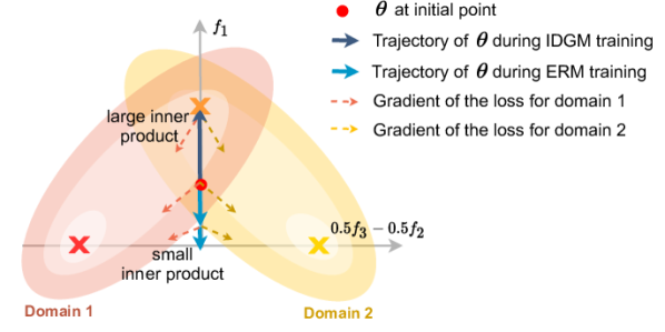
Figure 1: Isometric projection of training with ERM (blue) vs. our IDGM objective (dark blue), using data from Figure 2.

The goal of domain generalization is to train models that performs well on unseen, out-of-distribution data, which is crucial in practice for model deployment in the wild. This seemingly difficult task is made possible by the presence of multiple distributions/domains at train time. As we have seen in past work (Arjovsky et al., 2019, Gulrajani and Lopez-Paz, 2020, Ganin et al., 2016), a key aspect of domain generalization is to learn from features that remain invariant across multiple domains, while ignoring those that are spuriously correlated to label information (as defined in Torralba and Efros (2011), Stock and Cisse (2017)). Consider, for example, a model that is built to distinguish between cows and camels using photos collected in nature under different climates. Since CNNs are known to have a bias towards texture (Geirhos et al., 2018, Brendel and Bethge, 2019), if we simply try to minimize the average loss across different domains, the classifier is prone to spuriously correlate “cow” with grass and “camels” with desert, and predict the species using only the background. Such a classifier can be rendered useless when the animals are placed indoors or in a zoo. However, if the model could recognize that while the landscapes change with climate, the biological characteristics of the animals (e.g. humps, neck lengths) remain invariant and use those features to determine the species, we have a much better chance at generalizing to unseen domains.

Similar intuitions have already motivated several approaches that consider learning “invariances” accross domains as the main challenge of domain generalization. Most of these work focuses on learning invariant features, for instance domain adversarial neural networks (Ganin et al., 2016), CORAL (Sun and Saenko, 2016) and MMD for domain generalization (Li et al., 2018b). Different from previous approaches, invariant risk minimization (Arjovsky et al., 2019) proposes to learn intermediate features such that we have invariant predictor (when optimal) across different domains.

In this paper, we propose an inter-domain gradient matching (IDGM) objective. While our method also follows the invariance assumption, we are interested in learning a model with invariant gradient direction for different domains. Our IDGM objective augments the loss with an auxiliary term that maximizes the gradient inner product between domains, which encourages the alignment between the domain-specific gradients. By simultaneously minimizing the loss and matching the gradients, IDGM encourages the optimization paths to be the same for all domains, favouring invariant predictions. See Figure 1 for a visualization: given 2 domains, each containing one invariant feature (orange cross) and one spurious feature (yellow and red cross). While empirical risk minimisation (ERM) minimizes the average loss between these domains at the cost of learning spurious features only, IDGM maximizes the gradient inner product and is therefore able to focus on the invariant feature. Note that this plot is generated from an example, which we will describe in more details in Section 3.2.

While the IDGM objective achieves the desirable learning dynamic in theory, naive optimization of the objective by gradient descent is computationally costly due to the second-order derivatives. Leveraging the theoretical analysis of Reptile, a meta-learning algorithm (Nichol et al., 2018), we propose to approximate the gradients of IDGM using a simple first-order algorithm, which we name Fish. Fish is simple to implement, computationally effective and as we show in our experiments, functionally similar to direct optimization of IDGM.

Our contribution is a simple but effective training algorithm for domain generalization, which exhibits state-of-the-art performance on 13 datasets from recent domain generalization benchmark Wilds (Koh et al., 2020) and DomainBed. The strong performance of our method on a wide variety of datasets demonstrates that it is broadly applicable in different applications and subgenres of domain generalization problems. We also perform experiments to verify that our algorithm Fish does improve the normalized inter-domain gradient inner product, while this inner product decreases throughout training for ERM baseline.

2 Related Work

Domain Generalization In domain generalization, the training data is sampled from one or many source domains, while the test data is sampled from a new target domain. In contrast to domain adaptation, the learner does not have access to any data from the target domain (labeled or unlabeled) during train time (Quionero-Candela et al., 2009). In this paper we are interested in the scenario where multiple source domains are available, and the domain where the data comes from is known. Further, Koh et al. (2020) defines the datasets where train and test has disjoint domains “domain generalization”, and those where domains overlap between splits (but typically have different distributions) “subpopulation shift”. Following e.g., Gulrajani and Lopez-Paz (2020), in this paper we use domain generalization in a broader sense that encompasses the two categories.

We will now discuss the three main families of approaches to domain generalization:

1. Distributional Robustness (DRO): DRO approaches minimize the worst-case loss over a set of data distributions constructed from the training domains. Rojas-Carulla et al. (2015) proposed DRO to address covariate shift (Gretton et al., 2009a, b), where $P(Y|X)$ remains constant across domains but $P(X)$ changes. Later work also studied subpopulation shift, where the train and test distributions are mixtures of the same domains, but the mixture weights change between train and test (Hu et al., 2018, Sagawa et al., 2019);

2. Domain-invariant representation learning: This family of approaches to domain generalization aims at learning high-level features that make domains statistically indistinguishable. Prediction is then based on these features only. The principle is motivated by a generalization error bound for unsupervised domain adaptation (Ben-David et al., 2010, Ganin et al., 2016), but the approach readily applies to domain generalization (Gulrajani and Lopez-Paz, 2020, Koh et al., 2020). Algorithms include penalising the domain-predictive power of the model (Ganin et al., 2016, Wang et al., 2019, Huang et al., 2020), matching mean and variance of feature distributions across domains (Sun and Saenko, 2016), learning useful representations by solving Jigsaw puzzles (Carlucci et al., 2019) or using the maximum mean discrepancy (Gretton et al., 2006) to match the feature distributions (Li et al., 2018b).

   Similar to our approach, Koyama and Yamaguchi (2021) proposes IGA, which also adopts a gradient-alignment approach for domain generalization. The key difference between IGA and our IDGM objective is that IGA learns invariant features by minimizing the variance of inter-domain gradients. Notably, IGA is completely identical to ERM when ERM is the optimal solution on every training domain, since the variances of the gradients will be zero. While they achieve the best performance on the training set, both IGA and ERM could completely fail when generalizing to unseen domains (see Section 3.2 for such an example). Our method, on the contrary, biases towards non-ERM solutions as long as the gradients are aligned, and is therefore able to avoid this issue. Additionally, in Lopez-Paz and Ranzato (2017) we also see the application of gradient-alignment, however in this case it is applied under the continual learning setting to determine whether a gradient update will increase the loss of the previous tasks.

3. Invariant Risk Minimization (IRM): IRM is proposed by Arjovsky et al. (2019), which learns an intermediate representation such that the optimal classifiers (on top of this representation) of all domains are the same. The motivation is to exploit invariant causal effects between domains while reducing the effect of domain-specific spurious correlations.

Apart from these algorithms that are tailored for domain generalization, a well-studied baseline in this area is ERM, which simply minimizes the average loss over training domains. Using vanilla ERM is theoretically unfounded (Hashimoto et al., 2018, Blodgett et al., 2016, Tatman, 2017) since ERM is guaranteed to work only when train and test distributions match. Nonetheless, recent benchmarks suggest that ERM obtains strong performance in practice, in many case surpassing domain generalization algorithms (Gulrajani and Lopez-Paz, 2020, Koh et al., 2020). Our goal is to fill this gap, using an algorithm significantly simpler than previous approaches.

Connections to meta-learning

There are close connections between meta-learning (Thrun and Pratt, 1998) and (multi-source) domain adaptation. In fact, there are a few works in domain generalization that are inspired by the meta-learning principles, such as Li et al. (2018a), Balaji et al. (2018), Li et al. (2019), Dou et al. (2019).

Meta-learning aims at reducing the sample complexity of new, unseen tasks. A popular school of thinking in meta-learning is model agnostic meta-learning (MAML), first proposed in Finn et al. (2017), Andrychowicz et al. (2016). The key idea is to backpropagate through gradient descent itself to learn representations that can be easily adapted to unseen tasks. Our algorithmic solution is inspired by Reptile, a first-order approximation to MAML. However, our method has a fundamentally different goal, which is to exploit input-output correspondences that are invariant across domains. In contrast, meta-learning algorithms such as Reptile extract knowledge (e.g., input representations) that are useful to different tasks, but nothing has to be invariant across all tasks.

While our motivation is the exploitation of invariant features, similarly to IRM, our inter-domain gradient matching principle is an alternative to specifying hard constraints on the desired invariants across tasks. The resulting algorithm is both simple and efficient as it is a combination of standard gradient computations and parameter updates.

3 Methodology

3.1 Goals

Consider a training dataset $\mathcal{D}_{tr}$ consisting of $S$ domains $\mathcal{D}_{tr}=\{\mathcal{D}_{1},\cdots,\mathcal{D}_{S}\}$, where each domain $s$ is characterized by a dataset $\mathcal{D}_{s}:=\{(x^{s}_{i},y^{s}_{i})\}^{n_{s}}_{i=1}$ containing data drawn i.i.d. from some probability distribution. Also consider a test dataset $\mathcal{D}_{te}$ consisting of $T$ domains $\mathcal{D}_{te}=\{\mathcal{D}_{S+1},\cdots,\mathcal{D}_{S+T}\}$, where $\mathcal{D}_{tr}\cap\mathcal{D}_{te}=\emptyset$. The goal of domain generalization is to train a model with weights $\theta$ that generalizes well on the test dataset $\mathcal{D}_{te}$ such that:

$$\operatorname*{arg\,min}_{\theta}\operatorname{{}\mathbb{E}}_{\mathcal{D}\sim\mathcal{D}_{te}}\operatorname{{}\mathbb{E}}_{(x,y)\sim\mathcal{D}}\left[l((x,y);\theta)\right],$$ (1)

where $l((x,y);\theta)$ is the loss of model $\theta$ evaluated on $(x,y)$.

A naive approach is to emply ERM, which simply minimizes the average loss on $\mathcal{D}_{tr}$, ignoring the discrepancy between train and test domains:

$$\mathcal{L}_{\text{erm}}(\mathcal{D}_{tr};\theta)=\operatorname{{}\mathbb{E}}_{\mathcal{D}\sim\mathcal{D}_{tr}}\operatorname{{}\mathbb{E}}_{(x,y)\sim\mathcal{D}}\left[l((x,y);\theta)\right].$$ (2)

The ERM objective clearly does not exploit the input-output invariance across different domains in $\mathcal{D}_{tr}$ and could perform arbitrarily poorly on test data. We demonstrate this with a simple linear example as described in the next section.

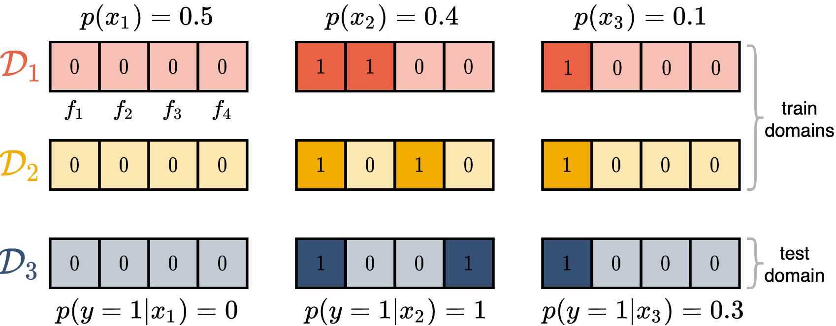
Figure 2: All domains contain 3 types of inputs $x_{1},x_{2}$ and $x_{3}$, each depicted in one column. 1^st col.: $x_{1}=[0,0,0,0]$, $y=0$, makes up for $50\%$ of each dataset; 2^nd col.: $x_{2}$ changes for each domain, $y=1$ always. $40\%$ of each dataset; 3^rd col.: $x_{3}=[1,0,0,0]$, $30\%$ of $y=1$ and $70\%$ of $y=0$. $10\%$ of each dataset.

3.2 The pitfall of ERM: a linear example

Consider a binary classification setup where data $(x,y)\in\mathbb{B}^{4}\times\mathbb{B}$, and a data instance is denoted $x=[f_{1},f_{2},f_{3},f_{4}],y$. Training data spans two domains $\{{\color[rgb]{0.73046875,0.33203125,0.234375}\mathcal{D}_{1}},{\color[rgb]{0.91015625,0.640625,0.12890625}\mathcal{D}_{2}}\}$, and test data one ${{\color[rgb]{0.03125,0.40234375,0.53515625}\mathcal{D}_{3}}}$. The goal is to learn a linear model $Wx+b=y,W\in\mathbb{R}^{4},b\in\mathbb{R}$ on the train data, such that the error on test data is minimized. The setup and dataset of this example is illustrated in Figure 2.

As we can see in Figure 2, $f_{1}$ is the invariant feature in this dataset, since the correlation between $f_{1}$ and $y$ is stable across different domains. The relationships between $y$ and $f_{2},f_{3}$ and $f_{4}$ changes for ${\color[rgb]{0.73046875,0.33203125,0.234375}\mathcal{D}_{1}}$, ${\color[rgb]{0.91015625,0.640625,0.12890625}\mathcal{D}_{2}}$, ${\color[rgb]{0.03125,0.40234375,0.53515625}\mathcal{D}_{3}}$, making them the spurious features. Importantly, if we consider one domain only, the spurious feature is a more accurate indicator of the label than the invariant feature. For instance, using $f_{2}$ to predict $y$ can give $97\%$ accuracy on ${\color[rgb]{0.73046875,0.33203125,0.234375}\mathcal{D}_{1}}$, while using $f_{1}$ only achieves $93\%$ accuracy. However, predicting with $f_{2}$ on ${\color[rgb]{0.91015625,0.640625,0.12890625}\mathcal{D}_{2}}$ and ${\color[rgb]{0.03125,0.40234375,0.53515625}\mathcal{D}_{3}}$ can at most reach $57\%$ accuracy, while $f_{1}$’s accuracy remains $93\%$ regardless of the domain.

Table 1: Performance comparison on the linear dataset.

Method	train acc.	test acc.	$W$	$b$
ERM	$97\%$	$57\%$	$[2.8,3.3,3.3,0.0]$	$-2.7$
IDGM	$93\%$	$93\%$	$[0.4,0.2,0.2,0.0]$	$-0.4$
Fish	$93\%$	$93\%$	$[0.4,0.2,0.2,0.0]$	$-0.4$

The performance of ERM on this simple example is shown in Table 1 (first row). From the trained parameters $W$ and $b$, we see that the model places most of its weights on spurious features $f_{2}$ and $f_{3}$. While this achieves the highest train accuracy ($97\%$), the model cannot generalize to unseen domains and performs poorly on test accuracy ($57\%$).

3.3 Inter-domain Gradient Matching (IDGM)

To mitigate the problem with ERM, we need an objective that learns from features that are invariant across domains. Let us consider the case where the train dataset consists of $S=2$ domains $\mathcal{D}_{tr}=\{\mathcal{D}_{1},\mathcal{D}_{2}\}$. Given model $\theta$ and loss function $l$, the expected gradients for data in the two domains is expressed as

$${G}_{1}=\operatorname{{}\mathbb{E}}_{\mathcal{D}_{1}}\frac{\partial l((x,y);\theta)}{\partial\theta},\quad{G}_{2}=\operatorname{{}\mathbb{E}}_{\mathcal{D}_{2}}\frac{\partial l((x,y);\theta)}{\partial\theta}.$$ (3)

The direction, and by extension, inner product of these gradients are of particular importance to our goal of learning invariant features. If $G_{1}$ and $G_{2}$ point in a similar direction, i.e. ${G}_{1}\cdot{G}_{2}>0$, taking a gradient step along ${G}_{1}$ or ${G}_{2}$ improves the model’s performance on both domains, indicating that the features learned by either gradient step are invariant across $\{\mathcal{D}_{1},\mathcal{D}_{2}\}$. This invariance cannot be guaranteed if ${G}_{1}$ and ${G}_{2}$ are pointing in opposite directions, i.e. ${G}_{1}\cdot{G}_{2}\leq 0$.

To exploit this observation, we propose to maximize the gradient inner product (GIP) to align the gradient direction across domains. The intended effect is to find weights such that the input-output correspondence is as close as possible across domains. We name our objective inter-domain gradient matching (IDGM), and it is formed by subtracting the inner product of gradients between domains $\widehat{G}$ from the original ERM objective. For the general case where $S\geq 2$, we can write

$$\mathcal{L}_{\text{idgm}} =\mathcal{L}_{\text{erm}}(\mathcal{D}_{tr};\theta)-\gamma\underbrace{\frac{2}{S(S-1)}\sum_{i,j\in S}^{i\neq j}{G}_{i}\cdot{G}_{j}}_{\text{GIP, denote as }\widehat{G}},$$ (4)

where $\gamma$ is the scaling term for $\widehat{G}$. Note that GIP can be computed in linear time as $\widehat{G}=||\sum_{i}G_{i}||^{2}-\sum_{i}||G_{i}||^{2}$ (ignoring the constant factor). We can also compute the stochastic estimates of Equation 4 by replacing out the expectations over the entire dataset by minibatches.

We test this objective on our simple linear dataset, and report results in the second row of Table 1. Note that to avoid exploding gradient we use the normalized GIP during training. The model has lower training accuracy compared to ERM ($93\%$), however its accuracy remains the same on the test set, much higher than ERM. The trained weights $W$ reveal that the model assigns the largest weight to the invariant feature $f_{1}$, which is desirable. The visualization in Figure 1 also confirms that by maximizing the gradient inner product, IDGM is able to focus on the feature that is common between domains, yielding better generalization performance than ERM.

3.4 Optimizing IDGM with Fish

The proposed IDGM objective, although effective, requires computing the second-order derivative of the model’s parameters due to the gradient inner product term, which can be computationally prohibitive. To mitigate this, we propose a first-order algorithm named Fish that approximates the optimization of IDGM with inner-loop updates. In Algorithm 1 we present Fish. As a comparison, we also present direct optimization of IDGM using SGD in Algorithm 2.

1:  for iterations = $1,2,\cdots$ do

2:     ${\widetilde{\theta}}\leftarrow\theta$

3:     for $\mathcal{D}_{i}\in\texttt{permute}(\{\mathcal{D}_{1},\mathcal{D}_{2},\cdots,\mathcal{D}_{S}\})$ do

4:        Sample batch ${d}_{i}\sim\mathcal{D}_{i}$

5:        $\displaystyle\widetilde{g}_{i}=\operatorname{{}\mathbb{E}}_{d_{i}}\left[\frac{\partial l((x,y);\widetilde{\theta})}{\partial{\widetilde{\theta}}}\right]$ /​​/Grad wrt $\widetilde{\theta}$

6:        Update ${\widetilde{\theta}}\leftarrow\widetilde{\theta}-\alpha\widetilde{g}_{i}$

7:     end for

8:     

9:     Update $\theta\leftarrow\theta+\displaystyle\epsilon(\widetilde{\theta}-\theta)$

10:  end for

Algorithm 1 Fish.

1:  for iterations = $1,2,\cdots$ do

2:     ${\widetilde{\theta}}\leftarrow\theta$

3:     for $\mathcal{D}_{i}\in\texttt{permute}(\{\mathcal{D}_{1},\mathcal{D}_{2},\cdots,\mathcal{D}_{S}\})$ do

4:        Sample batch ${d}_{i}\sim\mathcal{D}_{i}$

5:        $\displaystyle g_{i}=\operatorname{{}\mathbb{E}}_{d_{i}}\left[\frac{\partial l((x,y);\theta)}{\partial\theta}\right]$ /​​/Grad wrt $\theta$

6:        

7:     end for

8:     $\bar{g}=\displaystyle\frac{1}{S}\sum^{S}_{s=1}g_{s},\quad\widehat{g}=\overbrace{\frac{2}{S(S-1)}\sum_{i,j\in S}^{i\neq j}g_{i}\cdot g_{j}}^{\text{GIP (batch)}}$

9:     Update $\theta\leftarrow\theta-\epsilon\left(\bar{g}-\gamma(\partial\widehat{g}/\partial\theta)\right)$

10:  end for

Algorithm 2 Direct optimization of IDGM.

Fish performs $S$ inner-loop (l3-l7) update steps with learning rate $\alpha$ on a clone of the original model $\widetilde{\theta}$, and each update uses a minibatch $d_{i}$ from the domain selected in step $i$. Subsequently, $\theta$ is updated by a weighted difference between the cloned model and the original model $\epsilon(\widetilde{\theta}-\theta)$.

To see why Fish is an approximation to directly optimizing IDGM, we can perform Taylor-series expansion on its update in l8, Algorithm 1. Doing so reveals two leading terms: 1) $\bar{g}$: averaged gradients over inner-loop’s minibatches (effectively the ERM gradient); 2) $\partial\widehat{g}/\partial\theta$: gradient of the minibatch version of GIP. Observing l8 of Algorithm 2, we see that $\bar{g}$ and $\widehat{g}$ are actually the two gradient components used in direct optimization of IDGM. Therefore, Fish implicitly optimizes IDGM by construction (up to a constant factor), avoiding the computation of second-order derivative $\partial\widehat{g}/\partial\theta$. We present this more formally for the full gradient $G$ in Theorem 3.1.

Theorem 3.1

Given twice-differentiable model with parameters $\theta$ and objective $l$. Let us define the following:

$$G_{f} =\operatorname{{}\mathbb{E}}[(\theta-\widetilde{\theta})]-\alpha S\cdot\bar{G}, \alpha S\cdot$$ Fish update - ERM grad

$$G_{g} =-\partial\widehat{G}/\partial\theta, \max_{\theta}(\widehat{G})$$ grad of

where $\bar{G}=\frac{1}{S}\sum^{S}_{s=1}G_{s}$ and is the full gradient of ERM. Then we have

$$\lim_{\alpha\rightarrow 0}\frac{G_{f}\cdot G_{g}}{\left\lVert G_{f}\right\rVert\cdot\left\lVert G_{g}\right\rVert}=1.$$

Note that the expectation in $G_{f}$ is over the sampling of domains and minibatches. Theorem 3.1 indicates that when $\alpha$ is sufficiently small, if we remove the scaled ERM gradient component $\bar{G}$ from Fish’s update, we are left with a term $G_{f}$ that is in similar direction to the gradient of maximizing the GIP term in IDGM, which was originally second-order. Note that this approximation comes at the cost of losing direct control over the GIP scaling $\gamma$ — we therefore also derived a smoothed version of Fish that recovers this scaling term, however we find that changing the value of $\gamma$ does not make much difference empirically. See Appendix B for more details.

The proof to Theorem 3.1 can be found in Appendix A. We follow the analysis from Nichol et al. (2018), which proposes Reptile for model-agnostic meta-learning (MAML), where the relationship between inner-loop update and maximization of gradient inner product was first highlighted. Nichol et al. (2018) found the GIP term in their algorithm to be over minibatches from the same domain, which promoted within-task generalization; in Fish we construct inner-loop using minibatches over different domains – it therefore instead encourages across-domain generalization. We compare the two algorithms in further details in Section A.1.

We also train Fish on our simple linear dataset, with results in Table 1, and see it performs similarly to IDGM – the model assigns the most weight to the invariant feature $f_{1}$, and achieves $93\%$ accuracy on both train and test dataset.

4 Experiments

4.1 CdSprites-N

(a) Train

(b) Test

Figure 3: CdSprites-N train and test splits. Each 3x3 grid in train (e.g. yellow block) represents one domain.

Dataset We propose a simple shape-color dataset CdSprites-N based on the dSprites dataset (Matthey et al., 2017), which contains a collection of white 2D sprites of different shapes, scales, rotations and positions. CdSprites-N contains $N$ domains. The goal is to classify the shape of the sprites, and there is a shape-color deterministic matching that is specific per domain. This way we have shape as the invariant feature and color as the spurious feature. See Figure 3 for an illustration.

To construct the train split of CdSprites-N, we take a subset of dSprites that contains only 2 shapes (square and oval). We make $N$ replicas of this subset and assign 2 colors to each, with every color corresponding to one shape (e.g. yellow block in Figure 3(a), pink $\rightarrow$ squares, purple $\rightarrow$ oval). For the test split, we create another replica of the dSprites-N subset, and randomly assign one of the $2N$ colors in the training set to each shape in the test set.

We design this dataset with CNN’s texture bias in mind (Geirhos et al., 2018, Brendel and Bethge, 2019). If the value of $N$ is small enough, the model can simply memorize the $N$ colors that correspond to each shape, and make predictions solely based on colors, resulting in poor performance on the test set where color and shape are no longer correlated. Compared to other simple domain generalization datasets such as Digits-5 and Office-31, our dataset allows for precise control over the features that remains stable across domains and the features that change as domains change; we can also change the number of domains $N$ easily, making it possible to examine the effect $N$ has on the performance for domain generalization.

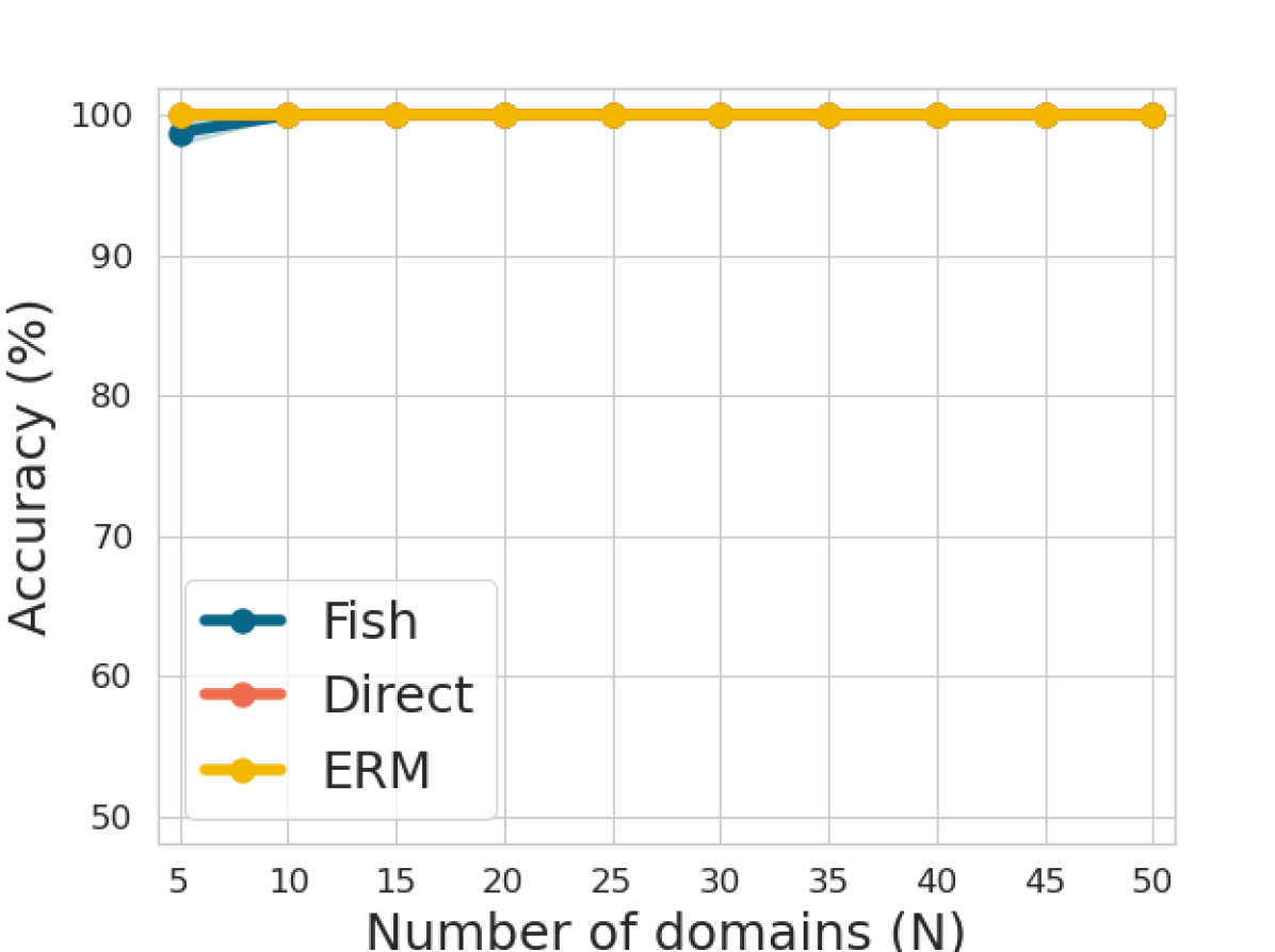
(a) Train

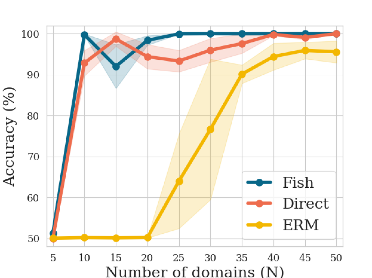
(b) Test

Figure 4: Performance on CdSprites-N, with $N\in[5,50]$

Results We train the same model using three different objectives including Fish, dicrect optimization of IDGM and ERM on this dataset with number of domains $N$ ranging from $5$ to $50$. Again, for direct optimization of IDGM, we use the normalized gradient inner product to avoid exploding gradient.

We plot the average train, test accuracy for each objective over 5 runs against the number of domains $N$ in Figure 4. We can see that the train accuracy is always $100\%$ for all methods regardless of $N$ (Figure 4(a)), while the test performance varies: Figure 4(b) shows that direct optimization of IDGM (red) and Fish (blue) obtain the best performances, with the test accruacy rising to over $90\%$ when $N\geq 10$ and near $100\%$ when $N\geq 20$. The predictions of ERM (yellow), on the other hand, remain nearly random on the test set up until $N=20$, and reach $95\%$ accuracy only for $N\geq 40$.

This experiment confirms the following: 1) the proposed IDGM objective have much stronger domain generalization capabilities compared to ERM; 2) Fish is an effective approximation of IDGM, with similar performance to its direct optimization. We also plot the gradient inner product progression of Fish vs. ERM during training in Figure 9(a), showing clearly that Fish does improve the gradient inner product across domain while ERM does not; 3) we also observe during training that Fish is about 10 times faster than directly optimizing IDGM, demonstrating its computational efficiency.

4.2 Wilds

Datasets We evaluate our model on the Wilds benchmark (Koh et al., 2020), which contains multiple datasets that capture real-world distribution shifts across a diverse range of modalities. We report experimental results on 6 challenging datasets in Wilds, and find Fish to outperform all baselines on most tasks. A summary on the Wilds datasets can be found in Table 2.

Table 2: A summary on Wilds datasets. See more details on the dataset in Appendix C.

Dataset	Domains	Metric	Disjoint	Architecture	# Train examples
Poverty	23 countries	Pearson (r)	✓	Resnet-18	10,000
Camelyon17	5 hospitals	Avg. acc.	✓	DenseNet-121	302,436
FMoW	16 years x 5 regions	Avg. & worst group acc.	✓	DenseNet-121	76,863
CivilComments	8 demographic groups	worst group acc.	✗	BERT	269,038
iWildCam	324 locations	Macro F1	✓	ResNet-50	142,202
Amazon	7,676 reviewers	10th percentile acc.	✓	BERT	1,000,124

For hyperparameters including learning rate, batch size, choice of optimizer and model architecutre, we follow the exact configuration as reported in the Wilds benchmark. Importantly, we also use the same model selection strategy used in Wilds to ensure a fair comparison. See details in Appendix D.

Table 3: Results on Wilds benchmark.

	PovertyMap		Camelyon17		FMoW		CivilComments		iWildCam		Amazon
	Pearson r		Avg. acc. (%)		Worst acc. (%)		Worst acc. (%)		Macro F1		10-th per. acc. (%)
Fish	0.80 ($\pm$1e-2)		74.7 ($\pm$7e-2)		34.6 ($\pm$0.00)		72.8 ($\pm$0.0)		22.0 ($\pm$0.0)		53.3 ($\pm$0.0)
IRM	0.78 ($\pm$3e-2)		64.2 ($\pm$8.1)		33.5 ($\pm$1.35)		66.3 ($\pm$2.1)		15.1 ($\pm$4.9)		52.4 ($\pm$0.8)
Coral	0.77 ($\pm$5e-2)		59.5 ($\pm$7.7)		31.0 ($\pm$0.35)		65.6 ($\pm$1.3)		32.8($\pm$0.1)		52.9 ($\pm$0.8)
Reweighted	-		-		-		66.2 ($\pm$1.2)		-		52.4 ($\pm$0.8)
GroupDRO	0.78 ($\pm$5e-2)		68.4 ($\pm$7.3)		31.4 ($\pm$2.10)		69.1 ($\pm$1.8)		23.9 ($\pm$2.1)		53.5 ($\pm$0.0)
ERM	0.78 ($\pm$3e-2)		70.3 ($\pm$6.4)		32.8 ($\pm$0.45)		56.0 ($\pm$3.6)		31.0 ($\pm$1.3)		53.8 ($\pm$0.8)
ERM (ours)	0.77 ($\pm$5e-2)		70.5 ($\pm$12.1)		30.9 ($\pm$1.53)		58.1 ($\pm$1.7)		25.1 ($\pm$0.2)		53.3 ($\pm$0.8)

Results See a summary of results in Table 3, where we use the metrics recommended in Wilds for each dataset. Again, following practices in Wilds, all results are reported over 3 random seed runs, apart from Camelyon17 which is reported over 10 random seed runs. We included additional results as well as a in-depth discussion on each dataset in Appendix C. We make the following observations:

1. Strong performance across datasets: Considering results on all 6 datasets, Fish is the best performing algorithm on Wilds. It outperforms all baseline on 4 datasets and achieves similar level of performance to the best method on the other 2 (Amazon and iWildCam). Fish’s strong performance on different types of data and architectures such as ResNet (He et al., 2016), DenseNet (Huang et al., 2017) and BERT (Devlin et al., 2018) demonstrated it’s capability to generalize to a diverse variety of tasks;

2. Strong performance on different domain generalization tasks: We make special note the CivilComments dataset captures subpopulation shift problems, where the domains in test are a subpopulation of the domains in train, while all other Wilds datasets depicts pure domain generalization problems, where the domains in train and test are disjointed. As a result, the baseline models for CivilComments selected by the Wilds benchmark are different from the methods used in all other datasets, and are tailored to avoiding systematic failure on data from minority subpopulations. We see that Fish works well in this setting too without any changes or special sampling strategies (used for baselines on CivilComments, see more in Table 10), demonstrating it’s capability to perform in different domain generalization scenarios;

3. Failure mode of domain generalization algorithms: We noticed that on iWildCam and Amazon, ERM is the best algorithm, outperforming all domain generalization algorithms except for Fish on Amazon. We believe that these domain generalization algorithms failed due to the large number of domains in these two datasets — 324 for iWildCam and 7,676 for Amazon. This is a common drawback of current domain generalization literature and is a direction worth exploring.

4.3 DomainBed

Table 4: Test accuracy ($\%$) on DomainBed benchmark.

	ERM	IRM	GroupDRO	Mixup	MLDG	Coral	MMD	DANN	CDANN	Fish (ours)
CMNIST	52.0 ($\pm$0.1)	51.8 ($\pm$0.1)	52.0 ($\pm$0.1)	51.9 ($\pm$0.1)	51.6 ($\pm$0.1)	51.7 ($\pm$0.1)	51.8 ($\pm$0.1)	51.5 ($\pm$0.3)	51.9 ($\pm$0.1)	51.6 ($\pm$0.1)
RMNIST	98.0 ($\pm$0.0)	97.9 ($\pm$0.0)	98.1 ($\pm$0.0)	98.1 ($\pm$0.0)	98.0 ($\pm$0.0)	98.1 ($\pm$0.1)	98.1 ($\pm$0.0)	97.9 ($\pm$0.1)	98.0 ($\pm$0.0)	98.0 ($\pm$0.0)
VLCS	77.4 ($\pm$0.3)	78.1 ($\pm$0.0)	77.2 ($\pm$0.6)	77.7 ($\pm$0.4)	77.1 ($\pm$0.4)	77.7 ($\pm$0.5)	76.7 ($\pm$0.9)	78.7 ($\pm$0.3)	78.2 ($\pm$0.4)	77.8 ($\pm$0.3)
PACS	85.7 ($\pm$0.5)	84.4 ($\pm$1.1)	84.1 ($\pm$0.4)	84.3 ($\pm$0.5)	84.8 ($\pm$0.6)	86.0 ($\pm$0.2)	85.0 ($\pm$0.2)	84.6 ($\pm$1.1)	82.8 ($\pm$1.5)	85.5 ($\pm$0.3)
OfficeHome	67.5 ($\pm$0.5)	66.6 ($\pm$1.0)	66.9 ($\pm$0.3)	69.0 ($\pm$0.1)	68.2 ($\pm$0.1)	68.6 ($\pm$0.4)	67.7 ($\pm$0.1)	65.4 ($\pm$0.6)	65.6 ($\pm$0.5)	68.6 ($\pm$0.4)
TerraInc	47.2 ($\pm$0.4)	47.9 ($\pm$0.7)	47.0 ($\pm$0.3)	48.9 ($\pm$0.8)	46.1 ($\pm$0.8)	46.4 ($\pm$0.8)	49.3 ($\pm$1.4)	48.7 ($\pm$0.5)	47.6 ($\pm$0.8)	45.1 ($\pm$1.3)
DomainNet	41.2 ($\pm$0.2)	35.7 ($\pm$1.9)	33.7 ($\pm$0.2)	39.6 ($\pm$0.1)	41.8 ($\pm$0.4)	41.8 ($\pm$0.2)	39.4 ($\pm$0.8)	38.4 ($\pm$0.0)	38.9 ($\pm$0.1)	42.7 ($\pm$0.2)
Average	67.0	66.0	65.5	67.1	66.8	67.2	66.8	66.4	66.1	67.1

Datasets While Wilds is a challenging benchmark capturing realistic distribution shift, to test our model under the synthetic-to-real transfer setting and provide more comparisons to SOTA methods, we also performed experiments on the DomainBed benchmark (Gulrajani and Lopez-Paz, 2020).

DomainBed is a testbed for domain generalization that implements consistent experimental protocols across SOTA methods to ensure fair comparison. It contains 7 popular domain generalization datasets, including Colored MNIST (Arjovsky et al., 2019), Rotated MNIST (Ghifary et al., 2015), VLCS (Fang et al., 2013), PACS (Li et al., 2017), OfficeHome (Venkateswara et al., 2017), Terra Incognita (Beery et al., 2018) and DomainNet (Peng et al., 2019), and offers comparison to a variety of SOTA domain generalization methods, including IRM (Arjovsky et al., 2019), Group DRO (Hu et al., 2018, Sagawa et al., 2019), Mixup (Yan et al., 2020), MLDG (Li et al., 2018a), Coral (Sun and Saenko, 2016), MMD (Li et al., 2018b), DANN (Ganin et al., 2016) and CDANN (Li et al., 2018).

Results Following recommendations in DomainBed, we report results using training domain as validation set for model selection. See results in Table 4, reported over 5 random trials. Averaging the performance over all 7 datasets, Fish ranks second out of 10 domain generalization methods. It performs only marginally worse than Coral (0.1$\%$), and is one of the three methods that performs better than ERM. This showcases Fish’s effectiveness on domain generalization datasets with stronger focus to synthetic-to-real transfer, which again demonstrates its versatility and robustness on different domain generalization tasks.

4.4 Analysis

Tracking gradient inner product In Figure 5, we demonstrate the progression of inter-domain gradient inner products during training using different objectives. We train both Fish (blue) and ERM (yellow) untill convergence while tracking the normalized gradient inner products between minibatches from different domains used in each inner-loop. To ensure a fair comparison, we use the exact same sequence of data for Fish and ERM (see Appendix H for more details).

Figure 5: Gradient inner product values during the training for CdSprites-N (N=15).

From Figure 5, it is clear that during training, the normalized gradient inner product of Fish increases, while that for ERM stays at the same value. The observations here shows that Fish is indeed effective in increasing/maintaining the level of inter-domain gradient inner product.

We conduct the same gradient inner product tracking experiments for the Wilds datasets we studied as well to shed some lights on its efficiency — see Appendix G for results.

Random Grouping We conducted experiments where data are grouped randomly instead of by domain for the inner-loop update. By doing so, we are still maximizing the inner product between minibatches, however it no longer holds that each minibatch contain data from one domain only. We therefore expect the results to be slightly worse than Fish, and the bigger the domain gap is, the more advantage Fish has against the random grouping strategy. We show the results for random grouping (Fish, RG) in Table 5.

Table 5: Ablation study on random grouping: test accuracy on different datasets.

	cDsprites(N=10)	FMoW	VLCS	PACS	OfficeHome
Fish	100.0 ($\pm$0.0)	34.3 ($\pm$0.6)	77.6 ($\pm$0.5)	85.5 ($\pm$0.3)	68.6 ($\pm$0.9)
Fish, RG	50.0 ($\pm$0.0)	33.4 ($\pm$1.7)	77.7 ($\pm$0.3)	83.9 ($\pm$0.7)	66.5 ($\pm$1.0)
ERM	50.0 ($\pm$0.0)	31.7 ($\pm$1.0)	77.5 ($\pm$0.4)	85.5 ($\pm$0.2)	66.5 ($\pm$0.3)

As expected, the random grouping strategy performs worse than Fish on all datasets. This is the most prominent on cDsprites with 10 domains (N=10), where Fish achieves $100\%$ test accuracy and both random grouping and ERM predicts randomly on the test split. The experiment demonstrated that the effectiveness of our algorithm largely benefited from the domain grouping strategy, and that maximising the gradient inner product between random batches of data does not achieve the same domain generalization performance.

Ablation studies on hyper-parameters We provide ablation studies on the learning rate of Fish’s inner-loop $\alpha$, meta step $\epsilon$, and number of inner loop steps $N$ in Appendix F. We also study the effect of fine-tuning on pretrained models at different stage of convergence in Appendix E.

5 Conclusion

In this paper we presented inter-domain gradient matching (IDGM) for domain generalization. To avoid costly second-order computations, we approximated IDGM with a simple first-order algorithm, Fish. We demonstrated our algorithm’s capability to learn from invariant features (as well as ERM’s failure to do so) using simple datasets such as CdSprites-N and the linear example. We then evaluated the model’s performance on Wilds and DomainBed, demonstrating that Fish performs well on different subgenres of domain generalization, and surpasses baseline performance on a diverse range of vision and language tasks using different architectures such as DenseNet, ResNet-50 and BERT. Our experiments can be replicated with 1500 GPU hours on NVIDIA V100.

Despite its strong performance, similar to previous work on domain generalization, when the number of domains is large Fish struggles to outperform ERM. We are currently investigating approaches by which Fish can be made to scale to datasets with orders of magnitude more domains and expect to report on this improvement in our future work.

Appendix A Taylor Expansion of Reptile and Fish Inner-loop Update

In this section we provide proof to Theorem 3.1. We reproduce and adapt the proof from Nichol et al. (2018) in the context of Fish, for completeness.

We demonstrate that when the inner-loop learning rate $\alpha$ is small, the direction of $G_{f}$ aligns with that of $G_{g}$, where

$$G_{f} =\operatorname{{}\mathbb{E}}\left[(\theta-\tilde{\theta})\right]-\alpha S\cdot\bar{G},$$ (5)

$$G_{g} =-\partial\widehat{G}/\partial\theta,$$ (6)

Expanding $G_{g}$

$G_{g}$ is the gradient of maximizing the gradient inner product (GIP).

$$G_{g}=-\frac{2}{S(S-1)}\sum_{i,j\in S}^{i\neq j}\frac{\partial}{\partial\theta}G_{i}\cdot G_{j}$$ (7)

Expanding $G_{f}$

To write out $G_{f}$, we need to derive the gradient update of Fish, $\theta-\tilde{\theta}$. Let us first define some notations.

For each inner-loop with $S$ steps of gradient updates, we assume a loss functions $l$ as well as a sequence of inputs $\{d_{i}\}_{i=1}^{S}$, where $d_{i}:=\{x_{b},y_{b}\}_{b=1}^{B}$ denotes a minibatch at step $i$ randomly drawn from one of the available domains in $\{\mathcal{D}_{1},\cdots,\mathcal{D}_{S}\}$. For reasons that will become clearer later, take extra note that the subscript $i$ here denotes the index of step, rather than the index of domain. We also define the following:

$$\widetilde{g}_{i}=\operatorname{{}\mathbb{E}}_{d_{i}}\left[\frac{\partial l((x,y);\theta_{i})}{\partial\theta_{i}}\right] i \theta_{i}$$ (gradient at step , wrt ) (8)

$$\theta_{i+1}=\theta_{i}-\alpha\widetilde{g}_{i}$$ (sequence of parameters) (9)

$$g_{i}=\operatorname{{}\mathbb{E}}_{d_{i}}\left[\frac{\partial l((x,y);\theta_{1})}{\partial\theta_{1}}\right] i \theta_{1}$$ (gradient at step , wrt ) (10)

$$H_{i}=\operatorname{{}\mathbb{E}}_{d_{i}}\left[\frac{\partial^{2}l((x,y);\theta_{1})}{\partial\theta_{1}^{2}}\right]$$ (Hessian at initial point) (11)

In the following analysis we omit the expectation $\operatorname{{}\mathbb{E}}_{d_{i}}$ and input $(x,y)$ to $l$ and instead denote the loss at step $i$ as $l_{i}$. Performing second-order Taylor approximation to $\widetilde{g}_{i}$ yields:

$$\widetilde{g}_{i} =l_{i}^{\prime}(\theta_{i})$$ (12)

$$=l_{i}^{\prime}(\theta_{1})+l_{i}^{\prime\prime}(\theta_{1})(\theta_{i}-\theta_{1})+\underbrace{\mathcal{O}(\lVert\theta_{i}-\theta_{1}\rVert^{2})}_{=\mathcal{O}(\alpha^{2})}$$ (13)

$$=g_{i}+H_{i}(\theta_{i}-\theta_{1})+\mathcal{O}(\alpha^{2})$$ (14)

$$=g_{i}-\alpha H_{i}\sum^{i-1}_{j=1}\widetilde{g}_{j}+\mathcal{O}(\alpha^{2}).$$ (15)

Applying first-order Taylor approximation to $\widetilde{g}_{j}$ gives us

$$\widetilde{g}_{j}=g_{j}+\mathcal{O}(\alpha),$$ (16)

plugging this back to Equation 15 yields:

$$\widetilde{g}_{i} =g_{i}-\alpha H_{i}\sum^{i-1}_{j=1}g_{j}+\mathcal{O}(\alpha^{2}).$$ (17)

For simplicity reason, let us consider performing two steps in inner-loop updates, i.e. $S=2$. We can then write the gradient of Fish $\theta-\tilde{\theta}$ as

$$\theta-\tilde{\theta} =\alpha(\widetilde{g}_{1}+\widetilde{g}_{2})$$ (18)

$$=\alpha(\underbrace{g_{1}+g_{2}}_{\scriptsize\leavevmode\hbox to8.9pt{\vbox to8.9pt{\text{[drawing]}}}})-\alpha^{2}\underbrace{H_{2}g_{1}}_{\scriptsize\leavevmode\hbox to8.9pt{\vbox to8.9pt{\text{[drawing]}}}}+\mathcal{O}(\alpha^{3}).$$ (19)

Furthermore, taking the expectation of $\theta-\tilde{\theta}$ under minibatch sampling gives us

$$=\operatorname{{}\mathbb{E}}_{1,2}\left[g_{1}+g_{2}\right]=G_{1}+G_{2}$$

$$=\operatorname{{}\mathbb{E}}_{1,2}\left[{H}_{2}g_{1}\right]=\operatorname{{}\mathbb{E}}_{1,2}\left[{H}_{1}g_{2}\right]$$ (interchanging indices)

$$=\frac{1}{2}\operatorname{{}\mathbb{E}}_{1,2}\left[{H}_{2}g_{1}+{H}_{1}g_{2}\right]$$ (averaging last two eqs)

$$=\frac{1}{2}\operatorname{{}\mathbb{E}}_{1,2}\left[\frac{\partial(g_{1}\cdot g_{2})}{\partial\theta_{1}}\right]$$

$$=\frac{1}{2}\cdot\frac{\partial(G_{1}\cdot G_{2})}{\partial\theta_{1}}$$

Note that the only reason we can interchange the indices in is because the subscripts represent steps in the inner loop rather than index of domains. Plugging , in Equation 19 yields:

$$\operatorname{{}\mathbb{E}}[\theta-\tilde{\theta}]=\alpha(G_{1}+G_{2})+\frac{\alpha^{2}}{2}\cdot\frac{\partial(G_{1}\cdot G_{2})}{\partial\theta_{1}}+\mathcal{O}(\alpha^{3})$$ (20)

We can also expand this to the general case where $S\geq 2$:

$$\operatorname{{}\mathbb{E}}[\theta-\tilde{\theta}]$$

$$\quad=\alpha\sum_{s=1}^{S}G_{s}-\frac{\alpha^{2}}{S(S-1)}\sum_{i,j\in S}^{i\neq j}\frac{\partial(G_{i}\cdot G_{j})}{\partial\theta_{1}}+\mathcal{O}(\alpha^{3}).$$ (21)

The second term in Equation 5 is $\bar{G}$, which is the full gradient of ERM defined as follow:

$$\bar{G}=\frac{1}{S}\sum^{S}_{s=1}G_{s}.$$ (22)

Plugging Equation 21 and Equation 22 to Equation 5 yields

$$G_{f} =\operatorname{{}\mathbb{E}}[\theta-\tilde{\theta}]-\alpha S\bar{G}$$ (23)

$$=-\frac{\alpha^{2}}{S(S-1)}\sum_{i,j\in S}^{i\neq j}\frac{\partial}{\partial\theta_{1}}G_{i}\cdot G_{j}$$ (24)

Comparing Equation 7 to Equation 24, we have:

$$\lim_{\alpha\rightarrow 0}\frac{G_{f}\cdot G_{g}}{\left\lVert G_{f}\right\rVert\left\lVert G_{g}\right\rVert}=1.$$

A.1 Fish and Reptile: Differences and Connections

As we introduced, our algorithm Fish is inspired by Reptile, a MAML algorithm.

Even though meta learning and domain generalization both study $N$-way, $K$-shot problems, there are some distinct differences that set them apart. The most prominent one is that in meta learning, some examples in the test dataset will be made available at test time ($K>0$), while in domain generalization no example in the test dataset is seen by the model ($K=0$); another important difference is that while domain generalization aims to train models that perform well on an unseen distribution of the same task, meta-learning assumes multiple tasks and requires the model to quickly learn an unseen task using only $K$ examples.

Due to these differences, it does not make sense in general to use MAML framework in domain generalization. As it turns out however, the idea of aligning gradients to improve generalization is relevant to both methods — The fundamental difference here that MAML algorithms such as Reptile aligns the gradients between batches from the same task Nichol et al. (2018), while Fish aligns those between batches from different tasks.

To see how this is ahiceved, let us have a look at the algorithmic comparison between Fish (blue) and Reptile (green) in Algorithm 3. As we can see, the key difference between the algorithm of Fish and Reptile is that Reptile performs its inner-loop using minibatches from the same task, while Fish uses minibatches from different tasks (l4-8). Based on the analysis in Nichol et al. (2018) (which we reproduce in Appendix A), this is why Reptile maximizes the within-task gradient inner products and Fish maximizes the across-task gradient inner products.

1:  for i = $1,2,\cdots$ do

2:     $\tilde{\theta}\leftarrow\theta$

3:      Sample task $\mathcal{D}_{t}\sim\{\mathcal{D}_{1},\cdots,\mathcal{D}_{T}\}$

4:     for ${\color[rgb]{0.36328125,0.51171875,0.4375}s\in\{1,\cdots,S\}}$ or ${\color[rgb]{0.03125,0.40234375,0.53515625}\mathcal{D}_{t}\in\{\mathcal{D}_{1},\cdots,\mathcal{D}_{T}\}}$ do

5:        Sample batch $\bm{d}_{t}\sim\mathcal{D}_{t}$

6:        $g_{t}=\partial\mathcal{L}(\bm{d}_{t};\tilde{\theta})/\partial\tilde{\theta}$

7:        Update $\tilde{\theta}\leftarrow\tilde{\theta}-\alpha g_{t}$

8:     end for

9:     Update $\theta\leftarrow\theta+\displaystyle\epsilon(\tilde{\theta}-\theta)$

10:  end for

Algorithm 3 Black fonts denote steps used in both algorithms, colored fonts are steps unique to Fish or Reptile.

A natural question to ask here is – how does this affect their empirical performance? In Figure 6, we show the train and test performance of Fish (blue) and Reptile (green) on CdSprites-N. We can see that despite the algorithmic similarity between Fish and Reptile, the two methods behave very differently on this domain generalization task: while Fish’s test accuracy goes to $100\%$ at $N=10$, Reptile’s test performance is always $50\%$ regardless of $N$. Moreover, we observe a dip in Reptile’s training performance early on, with the accuracy plateaus at $56\%$ when $N>20$. Reptile’s poor performance on this dataset is to be expected since its inner-loop is designed to encourage within-domain generalization, which is not helpful for learning what’s invariant across domains.

(a) Train

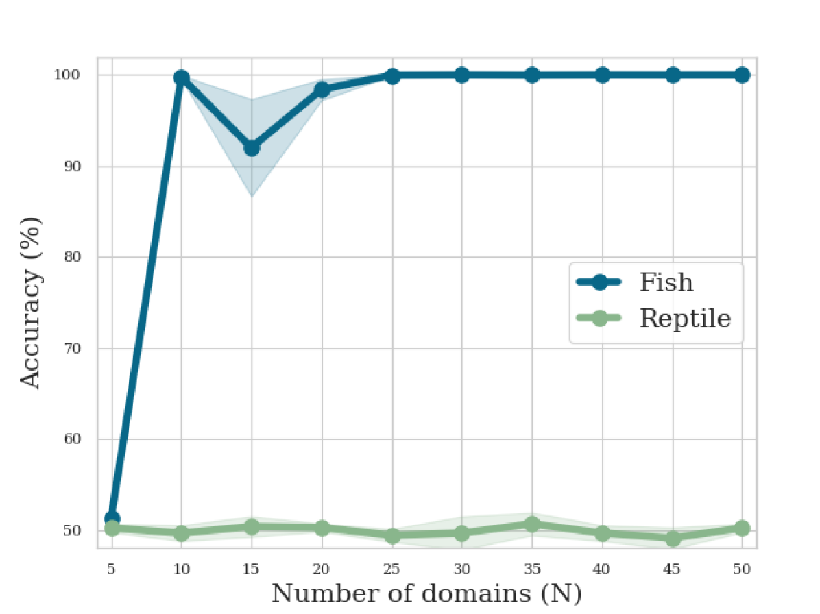
(b) Test

Figure 6: Performance on CdSprites-N, with $N\in[5,50]$

Appendix B SmoothFish: a more general algorithm

B.1 Derivation

We conclude in Appendix A that a component of Fish’s update $G_{f}=\operatorname{{}\mathbb{E}}[\theta-\tilde{\theta}]-\alpha S\cdot\bar{G}$ is in the same direction as the gradient of GIP, $G_{g}$. It is therefore possible to have explicit control over the scaling of the GIP component in Fish, similar to the original IDGM objective, by writing the following:

$$G_{\text{sm}}=\alpha S\cdot\bar{G}+\gamma\left(\operatorname{{}\mathbb{E}}[\theta-\tilde{\theta}]-\alpha S\cdot\bar{G}\right).$$ (25)

By introducing the scaling term $\gamma$, we have better control on how much the objective focus on inner product vs average gradient. Note that $\gamma=1$ recovers the original Fish gradient, and when $\gamma=0$ the gradient $G_{\text{sm}}$ is equivalent to ERM’s gradient with learning rate $\alpha S$. We name the resulting algorithm SmoothFish. See Algorithm 4.

1:  for iterations = $1,2,\cdots$ do

2:     ${\widetilde{\theta}}\leftarrow\theta$

3:     for $\mathcal{D}_{i}\in\texttt{permute}(\{\mathcal{D}_{1},\mathcal{D}_{2},\cdots,\mathcal{D}_{S}\})$ do

4:        Sample batch ${d}_{i}\sim\mathcal{D}_{i}$

5:        $\displaystyle g_{i}=\operatorname{{}\mathbb{E}}_{d_{i}}\left[\frac{\partial l((x,y);{\theta})}{\partial{{\theta}}}\right]$/​​/Grad wrt $\theta$

6:        $\displaystyle\widetilde{g}_{i}=\operatorname{{}\mathbb{E}}_{d_{i}}\left[\frac{\partial l((x,y);\widetilde{\theta})}{\partial{\widetilde{\theta}}}\right]$/​​/Grad wrt $\widetilde{\theta}$

7:        Update ${\widetilde{\theta}}\leftarrow\widetilde{\theta}-\alpha\widetilde{g}_{i}$

8:     end for

9:     $\bar{g}=\displaystyle\frac{1}{S}\sum_{s=1}^{S}g_{i},\ g_{\text{sm}}=\alpha S\bar{g}+\gamma\left((\widetilde{\theta}-\theta)-\alpha S\bar{g}\right)$

10:     Update $\theta\leftarrow\theta+\displaystyle\epsilon g_{\text{sm}}$

11:  end for

Algorithm 4 Smoothed version of Fish, which allows to get approximate gradients for the general form of Equation 4.

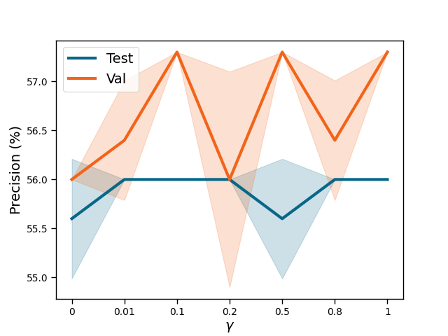
(a) Amazon

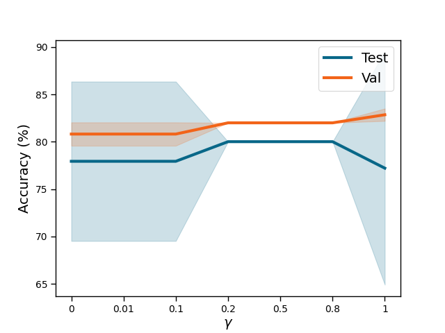
(b) Camelyon17

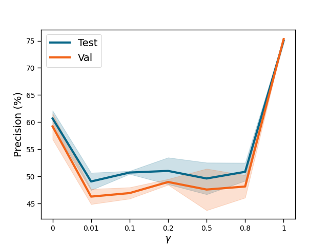
(c) CivilComments

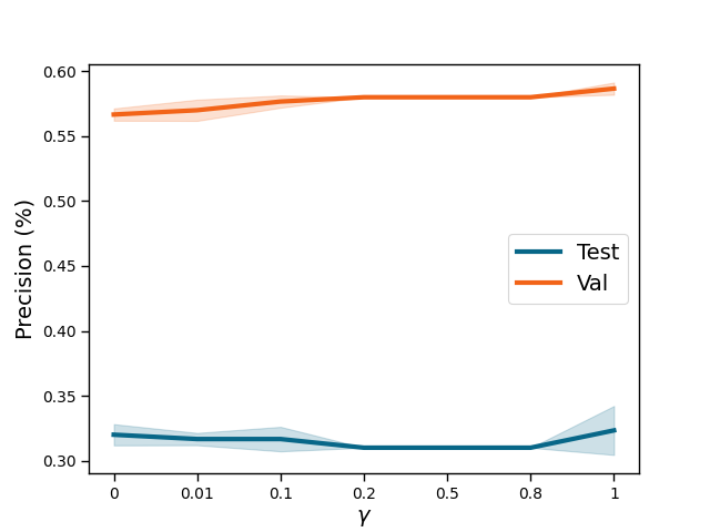
(d) FMoW

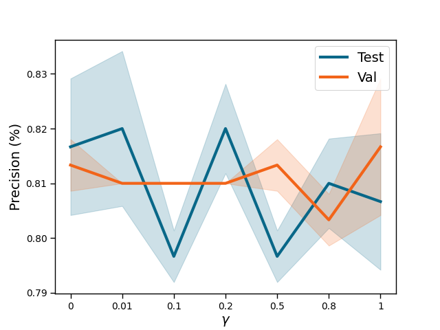
(e) Poverty

(f) iWildCam

Figure 7: Results on Wilds using SmoothFish with $\gamma$ ranging from 0 to 1.

B.2 Results

We run experiments on the 6 datasets in Wilds using SmoothFish, with $\gamma$ ranging in $[0.1,0.2,0.5,0.8]$. We also include results for $\gamma=0$ (equivalent to ERM) and $\gamma=1$ (equivalent to Fish). See results in Figure 7. The other hyperparameters including $\alpha$, meta steps, $\epsilon$ used here are the same as the ones used in our main experiments section.

Appendix C Discussions and Results on Wilds

We provide a more detailed summary of each dataset in Table 6. Some entries in $\#$ Domains are omitted because the domains in each split overlap. Note that in this paper we report the results on Wilds v1 — the benchmark has been updated since with slightly different dataset splits. We are currently working on updating our results to v2 of Wilds.

Table 6: Details of the 6 Wilds datasets we experimented on.

Dataset	Domains ($\#$ domains)	Data ($x$)	Target ($y$)	$\#$ Examples				$\#$ Domains
				train	val	test		train	val	test
FMoW	Time (16), Regions (5)	Satellite images	Land use (62 classes)	76,863	19,915	22,108		11, -	3, -	2, -
Poverty	Countries (23), Urban/rural (2)	Satellite images	Asset (real valued)	10,000	4,000	4,000		13, -	5, -	5, -
Camelyon17	Hospitals (5)	Tissue slides	Tumor (2 classes)	302,436	34,904	85,054		3	1	1
CivilComments	Demographics (8)	Online comments	Toxicity (2 classes)	269,038	45,180	133,782		-	-	-
iWildCam2020	Trap locations (324)	Photos	Animal species (186 classes)	142,202	20,784	38,943		245	32	47
Amazon	Reviewers (7,676)	Product reviews	Star rating (5 classes)	1,000,124	100,050	100,050		5,008	1,334	1,334

Table 7: Results on PovertyMap-Wilds.

Method	Val. Pearson r	Test Pearson r
Fish	0.81 ($\pm$6e-3)	0.81 ($\pm$9e-3)
IRM	0.81 ($\pm$4e-2)	0.78 ($\pm$3e-2)
ERM	0.80 ($\pm$3e-2)	0.78 ($\pm$3e-2)
ERM (ours)	0.80 ($\pm$3e-2)	0.77 ($\pm$5e-2)
Coral	0.80 ($\pm$4e-2)	0.77 ($\pm$5e-2)

Table 8: Results on Camelyon17-Wilds.

Method	Val. Accuracy ($\%$)	Test Accuracy ($\%$)
Fish	82.5 ($\pm$1.2)	79.5 ($\pm$6.0)
ERM	84.3 ($\pm$2.1)	73.3 ($\pm$9.9)
ERM (ours)	84.1 ($\pm$2.4)	70.5 ($\pm$12.1)
IRM	86.2 ($\pm$2.1)	60.9 ($\pm$15.3)
Coral	86.3 ($\pm$2.2)	59.2 ($\pm$15.1)

C.1 PovertyMap-Wilds

Task: Asset index prediction (real-valued). Domains: 23 countries

The task is to predict the real-valued asset wealth index of an area, given its satellite imagery. Since the number of domains considered here is large (23 countries), instead of looping over all $S$ domains in each inner-loop, we sample $N<<S$ domains in each iteration and perform inner-loop updates using minibatches from these domains only to speed up computation. For this dataset we choose $N=5$ by hyper-parameter search.

Evalutaion: Pearson Correlation (r). Following the practice in Wilds benchmark, we compare the results by computing Pearson correlation (r) between the predicted and ground-truth asset index over 3 random seed runs.

Results: We train the model using a ResNet-18 (He et al., 2016) backbone. See Table 7.

We see that Fish obtains the highest test performance, with the same validation performance as the best baseline. The performance is more stable between validation and test, and the standard deviation is smaller than for the baselines. We also report the results of ERM models trained in our environment as “ERM (ours)”, which shows similar performance to the canonical results reported in the Wilds benchmark itself (“ERM”).

C.2 Camelyon17-Wilds

Task: Tumor detection (2 classes). Domains: 5 hospitals

The Camelyon17-Wilds dataset contains 450,000 lymph-node scans from 5 hospitals. Due to the size of the dataset, instead of training with Fish from scratch, we pre-train the model with ERM using the recommended hyper-parameters in Koh et al. (2020), and fine-tune with Fish. For this dataset, we find that Fish performs the best when starting from a pretrained model that has not yet converged, achieving much higher accuracy than the ERM model. we provide an ablation study on this in Appendix E.

Evaluation: Average accuracy. We evaluate the average accuracy of this binary classification task. Following Koh et al. (2020), we show the mean and standard deviation of results over 10 random seeds runs. The number of random seeds required here is greater than other Wilds datasets due to the large variance observed in results. Note that these random seeds are not only applied during the fine-tuning stage, but also to the pretrained models to ensure a fair comparison.

Results: Following the practice in Wilds, we adopt DenseNet-121’s (Huang et al., 2017) architecture for models trained on this dataset. See results in Table 8.

The results show that Fish significantly outperforms all baselines – its test accuracy surpasses the best performing baseline by $6\%$. Also note that for all other baselines, there is a large gap between validation and test accuracy ($11\%\,\hstretch{0.9}{\vstretch{0.9}{\sim}}\,27\%$). This is because Wilds chose the hospital that is the most difficult to generalize to as the test split to make the task more challenging. Surprisingly, as we can observe in Table 8, the discrepancy between test and validation accuracy of Fish is quite small ($3\%$). The fact that it is able to achieve a similar level of accuracy on the worst-performing domain further demonstrates that Fish does not rely on domain-specific information, and instead makes predictions using the invariant features across domains.

Table 9: Results on FMoW-Wilds.

Method	Val. Accuracy ($\%$)			Test Accuracy ($\%$)
	Average	Worst		Average	Worst
Fish	57.3 ($\pm$0.01)	49.5 ($\pm$0.44)		51.8 ($\pm$0.12)	34.3 ($\pm$0.61)
ERM	59.7 ($\pm$0.14)	48.2 ($\pm$2.05)		53.1 ($\pm$0.25)	31.7 ($\pm$1.01)
ERM (ours)	59.9 ($\pm$0.22)	47.1 ($\pm$1.21)		52.9 ($\pm$0.18)	30.9 ($\pm$1.53)
IRM	57.2 ($\pm$0.01)	47.4 ($\pm$2.36)		50.9 ($\pm$0.32)	31.0 ($\pm$1.15)
Coral	56.7 ($\pm$0.06)	46.8 ($\pm$1.18)		50.5 ($\pm$0.30)	30.5 ($\pm$0.70)

Table 10: Results on CivilComments-Wilds.

Method	Val. Accuracy ($\%$)			Test Accuracy ($\%$)
	Average	Worst		Average	Worst
Fish	91.8 ($\pm$0.2)	75.3 ($\pm$0.3)		91.4 ($\pm$0.3)	74.2 ($\pm$0.5)
Group DRO	89.6 ($\pm$0.3)	68.7 ($\pm$1.0)		89.4 ($\pm$0.3)	70.4 ($\pm$2.1)
Reweighted	89.1 ($\pm$0.3)	67.9 ($\pm$1.2)		88.9 ($\pm$0.3)	67.3 ($\pm$0.1)
ERM	92.3 ($\pm$0.6)	53.6 ($\pm$0.7)		92.2 ($\pm$0.6)	58.0 ($\pm$1.2)
ERM (ours)	92.1 ($\pm$0.5)	54.1 ($\pm$0.4)		92.5 ($\pm$0.3)	58.1 ($\pm$1.7)

C.3 FMoW-Wilds

Task: Infrastructure classification (62 classes). Domains: 80 (16 years x 5 regions)

Similar to Camelyon17-Wilds, since the number of domains is large, we sample $N=5$ domains for each inner-loop. To speed up computation, we also use a pretrained ERM model and fine-tune with Fish; different from Section C.2, we find the best-performing models are acquired when using converged pretrained models (see details in Appendix E).

Evaluation: Average $\&$ worst-region accuracies. Following Wilds, the average accuracy evaluates the model’s ability to generalize over years, and the worst-region accuracy measures the model’s performance across regions under a time shift. We report results using 3 random seeds.

Results: Following Koh et al. (2020), we use a DenseNet-121 pretrained on ImageNet for this dataset. Results in Table 9 show that Fish has the highest worst-region accuracy on both test and validation sets. It ranks second in terms of average accuracy, right after ERM. Again, Fish’s performance is notably stable with the smallest standard deviation across all metrics compared to baselines.

C.4 CivilComments-Wilds

Task: Toxicity detection in online comments (2 classes). Domains: 8 demographic identities.

The CivilComments-Wilds contains 450,000 comments collected from online articles, each annotated for toxicity and the mentioning of demographic identities. Again, we use ERM pre-trained model to speed up computation, and sample $N=5$ domains for each inner-loop.

Evaluation: Worst-group accuracy. To study the bias of annotating comments that mentions demographic groups as toxic, the Wilds benchmark proposes to evaluate the model’s performance by doing the following: 1) Further separate each of the 8 demographic identities into 2 groups by toxicity – for example, separate black into black, toxic and black, not toxic; 2) measure the accuracies of these $8\times 2=16$ groups and use the lowest accuracy as the final evaluation of the model. This metric is equivalent to computing the sensitivity and specificity of the classifier on each demographic identity, and reporting the worse of the two metrics over all domains. Good performance on the group with the worst accuracy implies that the model does not tend to use demographic identity as an indicator of toxic comments.

Again, following Koh et al. (2020) we report results of 3 random seed runs.

Results: We compare results to the baselines used in the Wilds benchmark over 3 random seed runs in Table 10. All models are trained using BERT (Devlin et al., 2018).

The results show that Fish outperforms the best baseline by $4\%$ and $7\%$ on the test and validation set’s worst-group accuracy respectively, and is competitive in terms of average accuracy with ERM (within standard deviation). The strong performance of Fish on worst-group accuracy suggests that the model relies the least on demographic identity as an indicator of toxic comments compared to other baselines. ERM, on the other hand, has the highest average accuracy and the lowest worst-group accuracy. This indicates that it achieves good average performance by leveraging the spurious correlation between toxic comments and the mention of certain demographic groups.

Note that different from all other datasets in Wilds that focus on pure domain generalization (i.e, no overlap between domains in train and test splits), CivilComments-Wilds is a subpopulation shift problem, where the domains in test are a subpopulation of the domains in train. As a result, the baseline models used in Wilds for this dataset are different from the methods used in all other datasets, and are tailored to avoiding systematic failure on data from minority subpopulations. Fish works well in this setting too without any changes or special sampling strategies (such as $*$ and $+$ in Table 10). This further demonstrates the good performance of our algorithm on different domain generalization scenarios.

C.5 iWildCam-Wilds

Task: Animal species (186 classes). Domains: 324 camera locations.

The dataset consists of over 200,000 photos of animal in the wild, using stationary cameras across 324 locations. Classifying animal species from these heat or motion-activated photos is especially challenging: methods can easily rely on the background information of photos from the same camera setup. Fish models are pretrained with ERM till convergence, and for each inner loop we sample from $N=10$ domains.

Evaluation: Macro F1 score. Across the 186 class labels, we report average accuracy and both weighted and macro F1 scores (F1-w and F1-m, respectively, in Table 11). We run $3$ random seeds for each model.

Results: All models reported in Table 8 are trained using a ResNet-50. We find Fish to outperform baselines on both test accuracy and weighted F1, with a $1\%$ improvement on both metrics over the best performing model (ERM). However, this comes at the cost of lower macro F1 score, where Fish performs $1\%$ worse than ERM models that we trained and $3\%$ than the ERM reported in Wilds. This suggests that Fish is less good at classifying rarer species, however the overall accuracy on the test dataset is improved.

Although Fish did not outperform the ERM baseline on the primary evaluation metric proposed in Koh et al. (2020), we found the improvement of Fish in both accuracy and weighted F1 to be robust across a range of hyperparameters. See more details on this in Appendix D.

C.6 Amazon-Wilds

Task: Sentiment analysis (5 classes). Domains: 7,676 Amazon reviewers.

The dataset contains 1.4 million customer reviews on Amazon from 7,676 customers, and the task is to predict the score (1-5 stars) given the review. Similarly, we pretrained the model with ERM till convergence, and due to the large number of domains ($S=5008$ in train) we sample $N=5$ reviewers for each inner loop.

Evaluation: 10th percentile accuracy. Reporting the accuracy of the 10th percentile reviewer helps us assess whether the model performance is consistent across different reviewers. The results in Table 12 are reported over 3 random seeds.

Results: The model is trained using BERT (Devlin et al., 2018) backbone. While Fish has lower average accuracy compared to ERM, its 10th percentile accuracy matches that of ERM, outperforming all other baselines.

Table 11: Results on iWildCam-Wilds.

Method	Validation				Test
	Acc. (%)	Weighted F1	Macro F1		Acc. (%)	Weighted F1	Macro F1
Fish	58.0 ($\pm$0.2)	56.5 ($\pm$0.3)	25.8 ($\pm$0.5)		63.2 ($\pm$0.7)	64.0 ($\pm$0.5)	24.2 ($\pm$0.9)
Coral	-	-	-		62.5 ($\pm$1.7)	-	26.3 ($\pm$1.4)
ERM	-	-	-		62.9 ($\pm$0.5)	-	27.8 ($\pm$1.3)
ERM (ours)	55.8 ($\pm$0.2)	54.6 ($\pm$0.5)	27.7 ($\pm$1)		63.0 ($\pm$0.6)	62.4 ($\pm$0.2)	25.1 ($\pm$0.2)

Table 12: Results on Amazon-Wilds.

Method	Val. Accuracy ($\%$)			Test Accuracy ($\%$)
	Average	10-th per.		Average	10-th per.
Fish	73.8 ($\pm$0.1)	57.3 ($\pm$0.0)		72.9 ($\pm$0.2)	56.0 ($\pm$0.0)
ERM	74.3 ($\pm$0.0)	57.3 ($\pm$0.0)		73.5 ($\pm$0.1)	56.0 ($\pm$0.0)
ERM (ours)	74.0 ($\pm$0.0)	57.3 ($\pm$0.0)		73.3 ($\pm$0.1)	56.0 ($\pm$0.0)
IRM	73.6 ($\pm$0.2)	56.4 ($\pm$0.8)		73.3 ($\pm$0.2)	55.1 ($\pm$0.8)
Reweighted	69.6 ($\pm$0.0)	53.3 ($\pm$0.0)		69.2 ($\pm$0.1)	52.4 ($\pm$0.8)

Appendix D Hyperparameters

In Table 13 we list the hyperparameters we used to train ERM. The same hyperparameters were used for producing ERM baseline results and as pretrained models for Fish. In val. metric we report the metric on validation set that is used for model selection, and in cut-off we specify when to stop training when using ERM to generate pretrained models.

Table 13: Hyperparameters for ERM. We follow the hyperparameters used in Wilds benchmark. Note that we did not use a pretrained model for Poverty, therefore its cut-off condition is not reported.

Dataset	Model	Learning rate	Batch size	Weight decay	Optimizer	Val. metric	Cut-off
Camelyon17	Densenet-121	1e-3	32	0	SGD	acc. avg.	iter 500
CivilComments	BERT	1e-5	16	0.01	Adam	acc. wg.	Best val. metric
FMoW	Densenet-121	1e-4	64	0	Adam	acc. avg.	Best val. metric
iWildCam	Resnet-50	1e-4	16	0	Adam	F1-macro (all)	Best val. metric
Poverty	Resnet-18	1e-3	64	0	Adam	Pearson (r)	-
Amazon	BERT	2e-6	8	0.01	Adam	10th percentile acc.	-

In Table 14 we list out the hyperparameters we used to train Fish. Note that we train Fish using the same model, batch size, val metric and optimizer as ERM – these are not listed in Table 14 to avoid repetitions. Weight decay is always set as 0.

Table 14: Hyperparameters for Fish.

Dataset	Group by	$\alpha$	$\epsilon$	$\#$ domains	Meta steps
Camelyon17	Hospitals	1e-3	0.01	3	3
CivilComments	Demographics $\times$ toxicity	1e-5	0.05	16	5
FMoW	time $\times$ regions	1e-4	0.01	80	5
iWildCam	Trap locations	1e-4	0.01	324	10
Poverty	Countries	1e-3	0.1	23	5
Amazon	Reviewers	2e-6	0.01	7,676	5

Appendix E Ablation Studies on Pre-trained Models

In this section we perform ablation study on the convergence of pretrained ERM models. We study the performance of Fish with the following three configurations of pretrained ERM models:

1. Model is trained on $10\%$ of the data (epoch 1);

2. Model is trained on $50\%$ of the data (epoch 1);

3. Model at convergence.

By comparing the results between these three settings, we demonstrate how the level of convergence affects the Fish’s training performance. See results in Table 15. Note that Poverty is excluded here because the dataset is small enough that we are able to train Fish from scratch.

Table 15: Ablation study on pretrained ERM models.

Model	FMoW	Camelyon17	iWildCam	CivilComments
	Test Avg Acc	Test Avg Acc	Test Macro F1	Test Worst Acc
$10\%$ data	21.7 ($\pm$2.5)	79.1 ($\pm$12.3)	13.7 ($\pm$0.5)	71.8 ($\pm$1.3)
$50\%$ data	31.0 ($\pm$0.8)	64.6 ($\pm$12.3)	19.0 ($\pm$0.06)	74.2 ($\pm$0.5)
Converged	32.7 ($\pm$1.2)	63.5 ($\pm$8.2)	23.7 ($\pm$0.9)	73.8 ($\pm$1.8)

We see that CivilComments sustain good performance using pretrained models at different convergence levels. FMoW and iWildCam on the other hand seems to have strong preference towards converged model, and the results worsen as the amount of data seen during training goes down. Camelyon17 achieves the best performance when only $10\%$ of data is seen, and the test accuracy decreases while training with models with higher level of convergence.

Appendix F Ablation Studies on hyperparameters

$\alpha$ and $\epsilon$

We study the effect of changing Fish’s inner loop learning rate $\alpha$ and outer loop learning rate $\epsilon$. To make the comparisons more meaningful, we keep $\alpha\cdot\epsilon$ constant while changing their respective values. See results in Figure 8.

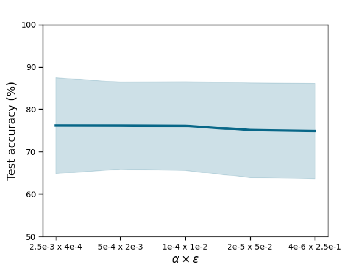
(a) Camelyon17

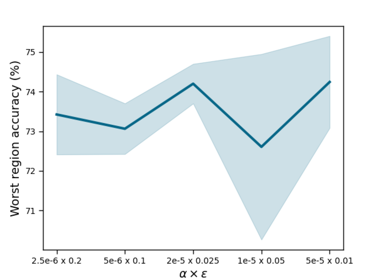
(b) CivilComments

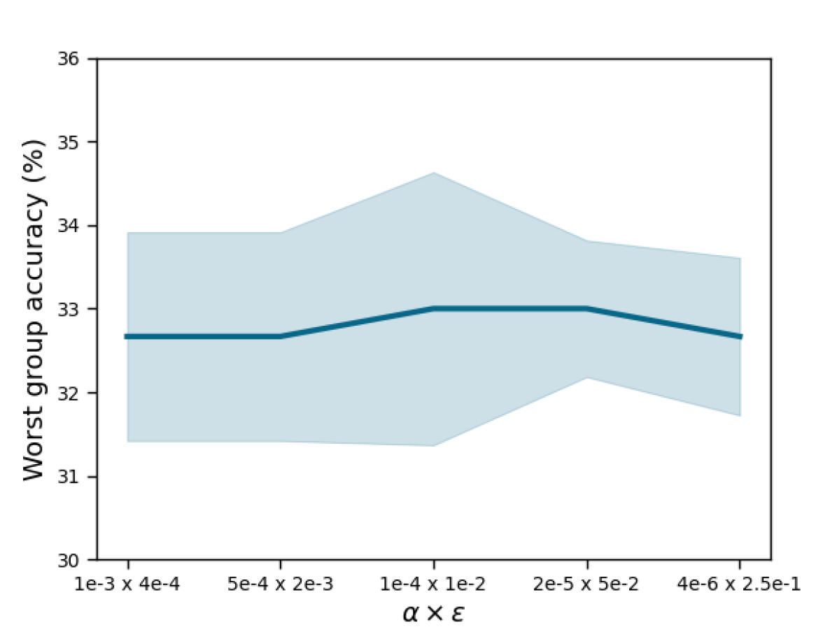
(c) FMoW

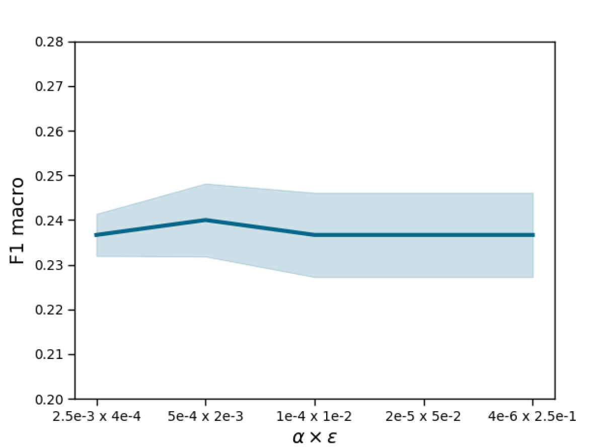
(d) iWildCam

(e) Poverty

Figure 8: Ablation studies on $\alpha$ and $\epsilon$. Note that $\alpha\times\epsilon$ remains constant in all experiments, and the midpoint of each plot is the hyperparameter we chose to use to report our experiment results.

Meta steps $N$

For most of the datasets we studied (all apart from Camelyon17 where $T=3$) we sample a $N$-sized subset of all $T$ domains available for training (see Table 14 for $T$ of each dataset). Here we study when $N=5,10,20$.

Table 16: Ablation study on meta steps $N$.

$N$	FMoW	Poverty	iWildCam	CivilComments
	Test Avg Acc	Test Pearson r	Test Macro F1	Test Worst Acc
$5$	33.0 ($\pm$1.6)	80.3 ($\pm$1.7)	23.7 ($\pm$0.9)	74.3 ($\pm$1.5)
$10$	32.7 ($\pm$1.2)	80.0 ($\pm$0.8)	23.7 ($\pm$0.5)	73.4 ($\pm$1.0)
$20$	33.3 ($\pm$2.1)	77.7 ($\pm$2.1)	23.7 ($\pm$0.9)	72.6 ($\pm$2.3)

In general altering these hyperparameters don’t have a huge impact on the model’s performance, however it does seem thet when $N=20$ the performance on some datasets (Poverty and CivilComments) degrade slightly.

Appendix G Tracking gradient inner product

(a) CdSprites-N

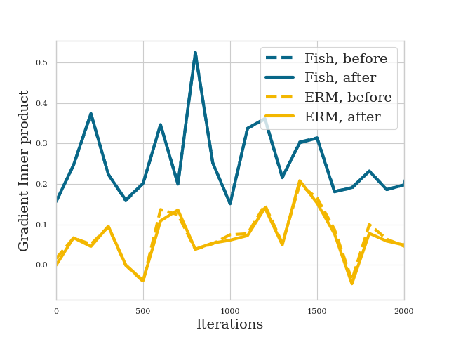
(b) Camelyon17

(c) CivilComments

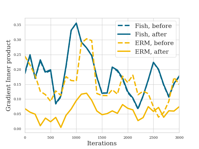
(d) FMoW

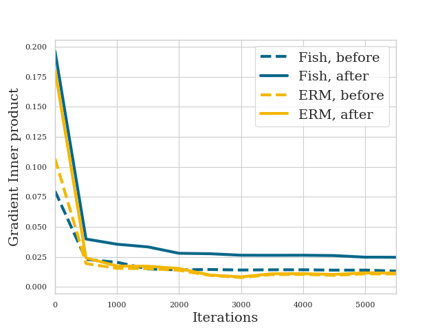
(e) Poverty

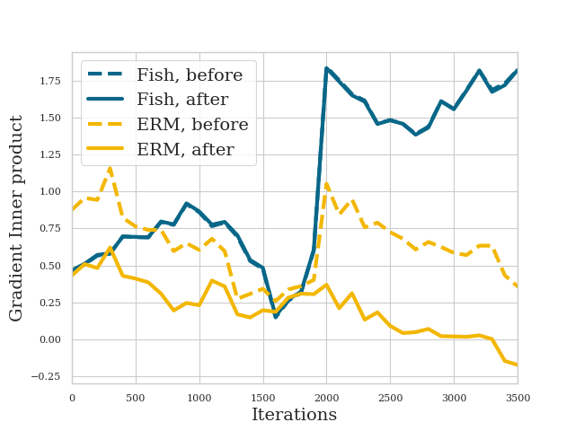
(f) iWildCam

Figure 9: Gradient inner product values during the training for CdSprites-N (N=15) and 5 different Wilds datasets.

In Figure 9, we demonstrate the progression of inter-domain gradient inner products during training using different objectives. We train both Fish (blue) and ERM (yellow) untill convergence while recording the normalized gradient inner products (i.e. cosine similarity) between minibatches from different domains used in each inner-loop. The gradient inner products are computed both before (dotted) and after (solid) the model’s update. To ensure a fair comparison, we use the exact same sequence of data for Fish and ERM (see Appendix H for more details).

Inevitably, the gradient inner product trends differently for each dataset since the data, types of domain splits and the choice of architecture are very different. In fact, the plot for CdSprites-N and Poverty are significantly different from others, with a dip in gradient inner product at the beginning of training – this is because these are the two datasets that we train from scratch. On all other datasets, the gradient inner products are recorded when fine-tuning with Fish.

Despite their differences, there are some important commonalities between these plots: if we compare the pre-update (dotted) to post-update (solid) curves, we can see that ERM updates often result in the decrease of gradient inner product, while for Fish it can either increase significantly (Figure 9(c) and Figure 9(e)) or at least stay at the same level (Figure 9(a), Figure 9(b), Figure 9(d) and Figure 9(f)). As a result of this, we can see that the post-update gradient inner product of Fish is always greater than ERM at convergence.

The observations here shows that Fish is effective in increasing/maintaining the level of inter-domain gradient inner product and sheds some lights on its efficiency on the datasets we studied.

Appendix H Algorithm for tracking gradient inner product

To make sure that the gradients we record for ERM and Fish are comparable, we use the same sequence of $S$-minibatches to train both algorithms. See Algorithm 6 for details.

1:  function $\texttt{{GIP}}(\{d_{1},d_{2},\cdots,d_{N}\},\theta)$:

2:  for $d_{n}\in\{d_{1},d_{2},\cdots,d_{N}\}$ do

3:     $g_{n}=\partial l(\bm{d}_{n};\theta)/\partial\theta$

4:  end for

5:  $\bar{\bar{\bm{g}}}=\frac{1}{S(S-1)}\sum_{i,j\in S}^{i\neq j}g_{i}\cdot g_{j}$

6:  return $\bar{\bar{\bm{g}}}$

Algorithm 5 Function GIP

1:  Initialize Fish $\theta_{f}\leftarrow\theta$, ERM $\theta_{e}\leftarrow\theta$

2:  for i = $1,2,\cdots$ do

3:     /​​/Get all minibatches

4:     for $\mathcal{D}_{n}\in\{\mathcal{D}_{1},\mathcal{D}_{2},\cdots,\mathcal{D}_{N}\}$ do

5:        Sample batch $\bm{d}_{n}\sim\mathcal{D}_{n}$

6:     end for

7:     /​​/GradInnerProd before update

8:     $\bar{\bar{\bm{g}}}_{Fb}=\texttt{GIP}(\{d_{1},d_{2},\cdots,d_{N}\}$, $\theta_{f}$)

9:     $\bar{\bar{\bm{g}}}_{Eb}=\texttt{GIP}(\{d_{1},d_{2},\cdots,d_{N}\}$, $\theta_{e}$)

10:     /​​/Fish training

11:     $\tilde{\theta}\leftarrow\theta_{f}$

12:     for $d_{n}\in\{d_{1},d_{2},\cdots,d_{N}\}$ do

13:        $g_{n}=\partial l(\bm{d}_{n};\tilde{\theta})/\partial\tilde{\theta}$

14:        Update $\tilde{\theta}\leftarrow\tilde{\theta}-\alpha g_{n}$

15:     end for

16:     $\theta_{f}\leftarrow\theta_{f}+\displaystyle\epsilon(\tilde{\theta}-\theta_{f})$

17:     /​​/Rearrange minibatches

18:     $d=\texttt{shuffle}(\texttt{concat}(d_{1},d_{2},\cdots,d_{N}))$

19:     $\{\tilde{d}_{1},\tilde{d}_{2},\cdots,\tilde{d}_{N}\}=\texttt{split}(d)$

20:     /​​/ERM training

21:     for $\tilde{d}_{n}\in\{\tilde{d}_{1},\tilde{d}_{2},\cdots,\tilde{d}_{N}\}$ do

22:        $g_{n}=\partial l(\tilde{d}_{n};\theta_{e})/\partial\theta_{e}$

23:        Update $\theta_{e}\leftarrow\theta_{e}-\alpha g_{n}$

24:     end for

25:     /​​/GradInnerProd after update

26:     $\bar{\bar{\bm{g}}}_{Fa}=\texttt{GIP}(\{d_{1},d_{2},\cdots,d_{N}\}$, $\theta_{f}$)

27:     $\bar{\bar{\bm{g}}}_{Ea}=\texttt{GIP}(\{d_{1},d_{2},\cdots,d_{N}\}$, $\theta_{e}$)

28:  end for

29:  Return $\bar{\bar{\bm{g}}}_{Fb}$, $\bar{\bar{\bm{g}}}_{Fa}$, $\bar{\bar{\bm{g}}}_{Eb}$, $\bar{\bar{\bm{g}}}_{Ea}$

Algorithm 6 Algorithm of collecting gradient inner product $\bar{\bar{\bm{g}}}$ for Fish and ERM both before and after updates. See GIP in Algorithm 5.

References

- Andrychowicz et al. (2016) M. Andrychowicz, M. Denil, S. Gomez, M. W. Hoffman, D. Pfau, T. Schaul, B. Shillingford, and N. De Freitas. Learning to learn by gradient descent by gradient descent. arXiv preprint arXiv:1606.04474, 2016.
- Arjovsky et al. (2019) M. Arjovsky, L. Bottou, I. Gulrajani, and D. Lopez-Paz. Invariant risk minimization. arXiv preprint arXiv:1907.02893, 2019.
- Balaji et al. (2018) Y. Balaji, S. Sankaranarayanan, and R. Chellappa. Metareg: towards domain generalization using meta-regularization. In NIPS’18 Proceedings of the 32nd International Conference on Neural Information Processing Systems, volume 31, pages 1006–1016, 2018.
- Beery et al. (2018) S. Beery, G. V. Horn, and P. Perona. Recognition in terra incognita. In Proceedings of the European Conference on Computer Vision (ECCV), pages 472–489, 2018.
- Ben-David et al. (2010) S. Ben-David, J. Blitzer, K. Crammer, A. Kulesza, F. Pereira, and J. W. Vaughan. A theory of learning from different domains. Machine learning, 79(1):151–175, 2010.
- Blodgett et al. (2016) S. L. Blodgett, L. Green, and B. T. O’Connor. Demographic dialectal variation in social media: A case study of african-american english. In Proceedings of the 2016 Conference on Empirical Methods in Natural Language Processing, pages 1119–1130, 2016.
- Brendel and Bethge (2019) W. Brendel and M. Bethge. Approximating cnns with bag-of-local-features models works surprisingly well on imagenet. In International Conference on Learning Representations (ICLR), 2019.
- Carlucci et al. (2019) F. M. Carlucci, A. D’Innocente, S. Bucci, B. Caputo, and T. Tommasi. Domain generalization by solving jigsaw puzzles. In 2019 IEEE/CVF Conference on Computer Vision and Pattern Recognition (CVPR), pages 2229–2238, 2019.
- Devlin et al. (2018) J. Devlin, M.-W. Chang, K. Lee, and K. N. Toutanova. Bert: Pre-training of deep bidirectional transformers for language understanding. In Proceedings of the 2019 Conference of the North American Chapter of the Association for Computational Linguistics: Human Language Technologies, Volume 1 (Long and Short Papers), pages 4171–4186, 2018.
- Dou et al. (2019) Q. Dou, D. C. de Castro, K. Kamnitsas, and B. Glocker. Domain generalization via model-agnostic learning of semantic features. In Advances in Neural Information Processing Systems, volume 32, pages 6450–6461, 2019.
- Fang et al. (2013) C. Fang, Y. Xu, and D. N. Rockmore. Unbiased metric learning: On the utilization of multiple datasets and web images for softening bias. In 2013 IEEE International Conference on Computer Vision, pages 1657–1664, 2013.
- Finn et al. (2017) C. Finn, P. Abbeel, and S. Levine. Model-agnostic meta-learning for fast adaptation of deep networks. In ICML’17 Proceedings of the 34th International Conference on Machine Learning - Volume 70, pages 1126–1135, 2017.
- Ganin et al. (2016) Y. Ganin, E. Ustinova, H. Ajakan, P. Germain, H. Larochelle, F. Laviolette, M. Marchand, and V. Lempitsky. Domain-adversarial training of neural networks. The journal of machine learning research, 17(1):2096–2030, 2016.
- Geirhos et al. (2018) R. Geirhos, P. Rubisch, C. Michaelis, M. Bethge, F. A. Wichmann, and W. Brendel. Imagenet-trained cnns are biased towards texture; increasing shape bias improves accuracy and robustness. In International Conference on Learning Representations (ICLR), 2018.
- Ghifary et al. (2015) M. Ghifary, W. B. Kleijn, M. Zhang, and D. Balduzzi. Domain generalization for object recognition with multi-task autoencoders. In 2015 IEEE International Conference on Computer Vision (ICCV), pages 2551–2559, 2015.
- Gretton et al. (2006) A. Gretton, K. Borgwardt, M. Rasch, B. Schölkopf, and A. Smola. A kernel method for the two-sample-problem. Advances in neural information processing systems, 19:513–520, 2006.
- Gretton et al. (2009a) A. Gretton, A. Smola, J. Huang, M. Schmittfull, K. Borgwardt, and B. Schölkopf. Covariate shift and local learning by distribution matching, pages 131–160. MIT Press, Cambridge, MA, USA, 2009a.
- Gretton et al. (2009b) A. Gretton, A. Smola, J. Huang, M. Schmittfull, K. Borgwardt, and B. Schölkopf. Covariate shift by kernel mean matching. Dataset shift in machine learning, 3(4):5, 2009b.
- Gulrajani and Lopez-Paz (2020) I. Gulrajani and D. Lopez-Paz. In search of lost domain generalization. arXiv preprint arXiv:2007.01434, 2020.
- Hashimoto et al. (2018) T. B. Hashimoto, M. Srivastava, H. Namkoong, and P. Liang. Fairness without demographics in repeated loss minimization. In International Conference on Machine Learning, pages 1929–1938, 2018.
- He et al. (2016) K. He, X. Zhang, S. Ren, and J. Sun. Deep residual learning for image recognition. In 2016 IEEE Conference on Computer Vision and Pattern Recognition (CVPR), pages 770–778, 2016.
- Hu et al. (2018) W. Hu, G. Niu, I. Sato, and M. Sugiyama. Does distributionally robust supervised learning give robust classifiers. In International Conference on Machine Learning, pages 2029–2037, 2018.
- Hu et al. (2018) W. Hu, G. Niu, I. Sato, and M. Sugiyama. Does distributionally robust supervised learning give robust classifiers? In International Conference on Machine Learning, pages 2029–2037. PMLR, 2018.
- Huang et al. (2017) G. Huang, Z. Liu, L. van der Maaten, and K. Q. Weinberger. Densely connected convolutional networks. In 2017 IEEE Conference on Computer Vision and Pattern Recognition (CVPR), pages 2261–2269, 2017.
- Huang et al. (2020) Z. Huang, H. Wang, E. P. Xing, and D. Huang. Self-challenging improves cross-domain generalization. In European Conference on Computer Vision, pages 124–140, 2020.
- Koh et al. (2020) P. W. Koh, S. Sagawa, H. Marklund, S. M. Xie, M. Zhang, A. Balsubramani, W. Hu, M. Yasunaga, R. L. Phillips, S. Beery, J. Leskovec, A. Kundaje, E. Pierson, S. Levine, C. Finn, and P. Liang. Wilds: A benchmark of in-the-wild distribution shifts. arXiv preprint arXiv:2012.07421, 2020.
- Koyama and Yamaguchi (2021) M. Koyama and S. Yamaguchi. Out-of-distribution generalization with maximal invariant predictor. In arXiv e-prints, 2021.
- Li et al. (2017) D. Li, Y. Yang, Y.-Z. Song, and T. M. Hospedales. Deeper, broader and artier domain generalization. In 2017 IEEE International Conference on Computer Vision (ICCV), pages 5543–5551, 2017.
- Li et al. (2018a) D. Li, Y. Yang, Y.-Z. Song, and T. Hospedales. Learning to generalize: Meta-learning for domain generalization. In Proceedings of the AAAI Conference on Artificial Intelligence, volume 32, 2018a.
- Li et al. (2019) D. Li, J. Zhang, Y. Yang, C. Liu, Y.-Z. Song, and T. Hospedales. Episodic training for domain generalization. In 2019 IEEE/CVF International Conference on Computer Vision (ICCV), pages 1446–1455, 2019.
- Li et al. (2018b) H. Li, S. J. Pan, S. Wang, and A. C. Kot. Domain generalization with adversarial feature learning. In Proceedings of the IEEE Conference on Computer Vision and Pattern Recognition, pages 5400–5409, 2018b.
- Li et al. (2018) Y. Li, X. Tian, M. Gong, Y. Liu, T. Liu, K. Zhang, and D. Tao. Deep domain generalization via conditional invariant adversarial networks. In Proceedings of the European Conference on Computer Vision (ECCV), pages 647–663, 2018.
- Lopez-Paz and Ranzato (2017) D. Lopez-Paz and M. Ranzato. Gradient episodic memory for continual learning. In Advances in Neural Information Processing Systems, volume 30, pages 6467–6476, 2017.
- Matthey et al. (2017) L. Matthey, I. Higgins, D. Hassabis, and A. Lerchner. dsprites: Disentanglement testing sprites dataset. https://github.com/deepmind/dsprites-dataset/, 2017.
- Nichol et al. (2018) A. Nichol, J. Achiam, and J. Schulman. On first-order meta-learning algorithms. arXiv: Learning, 2018.
- Peng et al. (2019) X. Peng, Q. Bai, X. Xia, Z. Huang, K. Saenko, and B. Wang. Moment matching for multi-source domain adaptation. In 2019 IEEE/CVF International Conference on Computer Vision (ICCV), pages 1406–1415, 2019.
- Quionero-Candela et al. (2009) J. Quionero-Candela, M. Sugiyama, A. Schwaighofer, and N. D. Lawrence. Dataset shift in machine learning. The MIT Press, 2009.
- Rojas-Carulla et al. (2015) M. Rojas-Carulla, B. Schölkopf, R. Turner, and J. Peters. A causal perspective on domain adaptation. stat, 1050:19, 2015.
- Sagawa et al. (2019) S. Sagawa, P. W. Koh, T. B. Hashimoto, and P. Liang. Distributionally robust neural networks for group shifts: On the importance of regularization for worst-case generalization. arXiv preprint arXiv:1911.08731, 2019.
- Sagawa et al. (2019) S. Sagawa, P. W. Koh, T. B. Hashimoto, and P. Liang. Distributionally robust neural networks for group shifts: On the importance of regularization for worst-case generalization. arXiv preprint arXiv:1911.08731, 2019.
- Stock and Cisse (2017) P. Stock and M. Cisse. Convnets and imagenet beyond accuracy: Explanations, bias detection, adversarial examples and model criticism. arXiv preprint arXiv:1711.11443, 2017.
- Sun and Saenko (2016) B. Sun and K. Saenko. Deep coral: Correlation alignment for deep domain adaptation. In European conference on computer vision, pages 443–450. Springer, 2016.
- Tatman (2017) R. Tatman. Gender and dialect bias in youtube’s automatic captions. In Proceedings of the First ACL Workshop on Ethics in Natural Language Processing, pages 53–59, 2017.
- Thrun and Pratt (1998) S. Thrun and L. Pratt, editors. Learning to Learn. Kluwer Academic Publishers, USA, 1998. ISBN 0792380479.
- Torralba and Efros (2011) A. Torralba and A. A. Efros. Unbiased look at dataset bias. In Proceedings of the 2011 IEEE Conference on Computer Vision and Pattern Recognition, CVPR ’11, page 1521–1528, USA, 2011. IEEE Computer Society. ISBN 9781457703942. doi: 10.1109/CVPR.2011.5995347. URL https://doi.org/10.1109/CVPR.2011.5995347.
- Venkateswara et al. (2017) H. Venkateswara, J. Eusebio, S. Chakraborty, and S. Panchanathan. Deep hashing network for unsupervised domain adaptation. In 2017 IEEE Conference on Computer Vision and Pattern Recognition (CVPR), pages 5385–5394, 2017.
- Wang et al. (2019) H. Wang, S. Ge, Z. C. Lipton, and E. P. Xing. Learning robust global representations by penalizing local predictive power. In Advances in Neural Information Processing Systems, volume 32, pages 10506–10518, 2019.
- Yan et al. (2020) S. Yan, H. Song, N. Li, L. Zou, and L. Ren. Improve unsupervised domain adaptation with mixup training. arXiv preprint arXiv:2001.00677, 2020.