Enhancement of microwave squeezing via parametric down-conversion in a superconducting quantum circuit

Abstract

We propose an experimentally accessible superconducting quantum circuit, consisting of two coplanar waveguide resonators (CWRs), to enhance the microwave squeezing via parametric down-conversion (PDC). In our scheme, the two CWRs are nonlinearly coupled through a superconducting quantum interference device embedded in one of the CWRs. This is equivalent to replacing the transmission line in a flux-driven Josephson parametric amplifier (JPA) by a CWR, which makes it possible to drive the JPA by a quantized microwave field. Owing to this design, the PDC coefficient can be considerably increased to be about tens of megahertz, satisfying the strong-coupling condition. Using the Heisenberg-Langevin approach, we numerically show the enhancement of the microwave squeezing in our scheme. In contrast to the JPA, our proposed system becomes stable around the critical point and can generate stronger transient squeezing. In addition, the strong-coupling PDC can be used to engineer the photon blockade.

I Introduction

Squeezing, i.e., the reduction of quantum fluctuations in one quadrature component at the expense of increasing fluctuations in the other canonically conjugate variable, is one of the extraordinary effects in quantum optics Walls83 ; Slusher85 ; Wu86 . Owing to the promising applications in, e.g., precision measurement Otterstrom14 ; Kruse2016 ; Malnou19 , quantum key distribution Garcia-Patron09 ; WangPu19 , engineering matter interactions Lv15 ; Zeytinoglu17 ; Qin18 and improving the efficiency of heat engines Klaers17 ; Wang19 , the generation of squeezed light has attracted much attention. Up to now, numerous schemes for squeezing have been proposed, typically using the optomechanical interaction Fabre94 ; Xiao14 ; Yu18 , the four-wave mixing Slusher85 , and the degenerate parametric down-conversion (PDC) Wu86 . Here, the degenerate PDC involves a three-wave mixing process of generating a lower-energy photon pair with the same frequency by splitting a higher-energy photon via a nonlinear medium Walls94 .

On the other hand, fast developments of the superconducting quantum circuits (SQCs) have greatly facilitated the progress in quantum information processing (see. e.g., Devoret1169 ; You11 ; Wendin_2017 ; Tsai_2021 ). Since the SQCs based on Josephson junctions can be designed and fabricated to tailor their characteristics for various purposes, they have also been used as the platforms for exploring quantum-optics phenomena in the microwave domain You11 . For instance, electromagnetically induced transparency and Autler-Townes splitting Li15 ; Novikov16 ; Long18 ; Chien19 , sideband transitions Diaz16 ; Chen2017 ,quantum entanglement Wei2006 ; Neeley2010 ; White2016 ; Armata17 ; Izmalkov04 ; Zippilli15 , Bloch-Siegert shifts Diaz10 ; Wang20 and superradiant quantum phase transitions Feng15 ; Xiang16 ; Motoaki16 ; Garziano14 were demonstrated using the SQCs. Also, the generation of squeezed microwaves via, e.g., degenerate four-wave mixing and degenerate PDC was proposed theoretically and later realized experimentally Yurke89 ; Cao11 ; Benlloch14 ; Zhong_2013 ; Moon05 ; Wang15 . Most importantly, the advantage of easy tunability in SQCs makes it promising to demonstrate and manipulate more quantum-optics phenomena in the microwave domain.

In this paper, we propose an experimentally feasible scheme to obtain squeezed microwaves via quantized-field-driven PDC in a SQC. The considered system is composed of two superconducting coplanar waveguide resonators (CWRs), denoted as CWR-A and CWR-B, which are inductively coupled to each other by a superconducting quantum interference device (SQUID) embedded in CWR-A. The magnetic flux threading the SQUID loop contains the externally applied magnetic flux and the quantized magnetic flux generated by the current in CWR-B. This is equivalent to replacing the transmission line in a flux-driven Josephson parametric amplifier (JPA) with a CWR (i.e., the CWR-B), which makes it possible to drive the JPA by a quantized microwave field. A similar method was also used in the optical parametric amplifier to enhance the squeezing by embedding the nonlinear crystal in an optical cavity Vahlbruch16 , where the nonlinear crystal and the optical cavity play similar roles as the nonlinear CWR-A (i.e., the JPA) and the CWR-B in our proposed system, respectively. The generated quantized magnetic flux modulates the phase across the SQUID and gives rise to the mutual coupling between the two resonators. The SQUID usually works in the phase regime where the phase degree of freedom dominates. When the external magnetic field is much stronger than the generated quantized magnetic field, the coupled SQC system can be described by a PDC Hamiltonian, where the classical drive field in the JPA is replaced by a quantized drive field. With this quantized-field-driven PDC Hamiltonian, we study the microwave squeezing in the proposed system. In fact, due to the nonlinearity of the Josephson junction, a small SQUID is a highly nonlinear system. Therefore, we can use it to explore the high-order nonlinear effect of the SQUID on the microwave squeezing in our SQC system.

Around a critical drive strength, our proposed system is stable and can produce optimum steady-state squeezing. This is different from a flux-driven JPA Zhong_2013 , which can have the same degree of steady-state squeezing, but is unstable around the critical point, yielding the optimum steady-state squeezing experimentally inaccessible. Moreover, for the JPA, its transient squeezing cannot exceed the steady-state squeezing, while our scheme does not have this limitation and stronger transient squeezing can be achieved (cf. Sec. III). Also, compared with the microwave squeezing in Refs. Moon05 ; Wang15 , our proposal has distinct advantages. First, the design we present here is non-dispersive and directly interacted. This is in contrast to other proposals based on dispersive and indirect couplings via couplers Moon05 ; Wang15 . While in those works the nonlinear coupling strength (which is only tens of kilohertz) is much limited by the dispersive condition, our setup can increase the nonlinear coupling strength by three orders of magnitude. This promises an appreciable enhancement of the microwave squeezing in the proposed circuit. Second, our setup with the SQUID can be easily fabricated as well, since the needed technology has been maturely utilized for other experiments Baust15 . In addition, our scheme may have other potential applications in quantum technologies. For example, the nonlinear coupling strength in our scheme is larger than the decay rates of CWRs (usually smaller than one megahertz Xiang13 ), so a strong coupling can be realized between the two CWRs. Contrary to the weak-coupling regime, the photon blockade becomes accessible in this strong-coupling regime Zhou2020 .

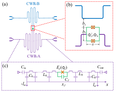
Figure 1: (a) Schematic of the proposed SQC system consisting of two CWRs denoted as CWR-A and CWR-B, which are nonlinearly coupled to each other via a SQUID (green dot) embedded in CWR-A. (b) An enlarged view of the part denoted by a red rectangular in (a). (c) The lumped-element circuit of CWR-A, where the SQUID is located at $x=x_{J}$.

II Proposed circuit

As illustrated in Fig. 1(a), the proposed SQC system is composed of two CWRs (i.e., CWR-A and CWR-B), where both resonators are inductively coupled to each other via a SQUID embedded in CWR-A. Below we first derive CWR-A’s Hamiltonian and then give the Hamiltonian of the proposed SQC system.

II.1 Nonlinear resonator

Due to the SQUID embedded, CWR-A is a nonlinear resonator, which can act as a JPA in the regime with appropriate parameters Zhong_2013 . We assume CWR-A to be of a length $2l_{a}$ and decompose it into lumped-circuit elements, as shown in Fig. 1(c). For simplicity and without loss of generality, we also assume that the two resonators have the same capacitance $C_{0}$ per unit length and the same inductance $L_{0}$ per unit length. When the SQUID is excluded, the Lagrangian of the bare resonator for CWR-A can be written as

$$\mathcal{L}^{\prime}_{a}=\int_{-l_{a}}^{l_{a}}\bigg{[}\frac{C_{0}}{2}\dot{\Phi}^{2}(x,t)-\frac{[\partial_{x}\Phi(x,t)]^{2}}{2L_{0}}\bigg{]}dx,$$ (1)

where $\Phi(x,t)=\int_{-\infty}^{t}V(x,t^{\prime})dt^{\prime}$ is the magnetic flux and $V(x,t^{\prime})$ is the voltage. For a symmetric SQUID with $C_{J1}=C_{J2}=C_{J}/2$ and $E_{J1}=E_{J2}=E_{J}/2$, the effective Josephson energy is $E_{J}(\Phi_{e})=E_{J}\cos(\pi\Phi_{e}/\Phi_{0})$, where $\Phi_{0}=h/(2e)$ is the flux quantum. The total magnetic flux $\Phi_{e}$ threading the SQUID loop is composed of the externally applied magnetic flux $\Phi^{\prime}_{e}$ and the magnetic flux $\Phi_{b}$ generated by the current in CWR-B, i.e., $\Phi_{e}=\Phi^{\prime}_{e}+\Phi_{b}$, where the small magnetic flux induced by the self inductance of the SQUID loop is neglected. Under the condition $\Phi^{\prime}_{e}\gg\Phi_{b}$, the change of the effective Josephson energy $E_{J}(\Phi_{e})$ due to the magnetic flux $\Phi_{b}$ can be linearly approximated as $E_{J}(\Phi_{e})\approx E_{J}(\Phi^{\prime}_{e})[1-\tan(\pi\Phi^{\prime}_{e}/\Phi_{0})(\pi\Phi_{b}/\Phi_{0})]$. This approximation is reasonable because $0.25\leq\Phi^{\prime}_{e}/\Phi_{0}\leq 0.45$ and $\Phi_{b}/\Phi_{0}\sim 1\times 10^{-3}$ in our paper.

The Lagrangian of the SQUID takes the standard form $\mathcal{L}_{S}=C_{J}\dot{\delta}^{2}/2-E_{J}(\Phi_{e})\big{[}1-\cos(2\pi\delta/\Phi_{0})\big{]}$, where $\delta=\Phi(x_{J}^{+},t)-\Phi(x_{J}^{-},t)$ is the phase drop of the SQUID located at $x=x_{J}$ [see Fig. 1(c)]. Another important parameter of the SQUID is the effective charge energy $E_{C}=(2e)^{2}/(2C_{J})$. When the SQUID is in the phase regime, i.e., $E_{J}(\Phi_{e})\gg E_{C}$, we expand the cosine potential of the SQUID up to the fourth order of $2\pi\delta/\Phi_{0}$. The Lagrangian $\mathcal{L}_{S}$ can be approximately written as $\mathcal{L}_{S}=\mathcal{L}_{S}^{(2)}+\mathcal{L}_{S}^{(3)}+\mathcal{L}_{S}^{(4)}$, where

$$\mathcal{L}_{S}^{(2)} =\frac{C_{J}}{2}\dot{\delta}^{2}-\frac{\delta^{2}}{2L_{J}},$$

$$\mathcal{L}_{S}^{(3)} =\frac{\delta^{2}}{2L_{J}}\bigg{(}\pi\frac{\Phi_{b}}{\Phi_{0}}\bigg{)}\tan\bigg{(}\frac{\pi\Phi^{\prime}_{e}}{\Phi_{0}}\bigg{)},$$

$$\mathcal{L}_{S}^{(4)} =\frac{\delta^{4}}{24L_{J}}\bigg{(}\frac{2\pi}{\Phi_{0}}\bigg{)}^{2},$$ (2)

with the Josephson inductance $L_{J}$ defined by $1/L_{J}=(2\pi/\Phi_{0})^{2}E_{J}(\Phi^{\prime}_{e})$. The quality factor of the resonator for CWR-A is assumed to be sufficiently high, so we can consider the limiting case $C_{\rm in,out}\rightarrow 0$, which corresponds to the open-ended boundary condition Johansson14

$$\partial_{x}\Phi(x,t)|_{x=-l_{a}}=\partial_{x}\Phi(x,t)|_{x=l_{a}}=0,$$ (3)

where $C_{\rm in}$ and $C_{\rm out}$ are the capacitances of the input and output capacitors at the two ends of CWR-A. Moreover, according to Kirchhoff’s current law, around $x=x_{J}$, we have

$$\frac{1}{L_{0}}\partial_{x}\Phi(x,t)|_{x=x_{J}^{-}}=\frac{1}{L_{0}}\partial_{x}\Phi(x,t)|_{x=x_{J}^{+}}=C_{J}\ddot{\delta}+\frac{\delta}{L_{J}},$$ (4)

due to the presence of the SQUID in the resonator Bourassa12 .

First, we study the normal modes of CWR-A and quantize the Hamiltonian related to the linear Lagrangian $\mathcal{L}_{a}=\mathcal{L}^{\prime}_{a}+\mathcal{L}_{S}^{(2)}$, where higher-order nonlinear terms in the Lagrangian $\mathcal{L}_{S}$ are ignored. As shown in Appendix A, by using the method of separating variables under the conditions in Eqs. (3) and (4), the linear Lagrangian $\mathcal{L}_{a}$ of CWR-A can be written as $\mathcal{L}_{a}=\sum_{m}[C_{\Sigma}\dot{\phi}_{m}^{2}/2-\phi_{m}^{2}/2L_{m}]$. Here $C_{\Sigma}\equiv 2C_{0}l_{a}+C_{J}$ is the total capacitance and $L_{m}$ is the effective inductance related to the $m$th mode of CWR-A. Both the flux amplitude $\phi_{m}$ and the spatial mode function $\mu_{m}(x)$ of the $m$th mode satisfy $\Phi(x,t)=\sum_{m}\phi_{m}(t)\mu_{m}(x)$. With a Legendre transformation, the Hamiltonian $H_{a}$ of CWR-A is obtained as

$$H_{a}=\sum_{m}\bigg{[}\frac{p_{m}^{2}}{2C_{\Sigma}}+\frac{\phi_{m}^{2}}{2L_{m}}\bigg{]},$$ (5)

where $p_{m}=C_{\Sigma}\dot{\phi}_{m}$ is the canonical momentum of the $m$th mode, conjugate to the canonical coordinate $\phi_{m}$. We treat the canonical variables $\phi_{m}$ and $p_{m}$ as quantum operators satisfying the commutation relation $[\phi_{n},p_{m}]=i\hbar\delta_{nm}$ and can then write them as

$$\phi_{m} =\sqrt{\frac{\hbar}{2C_{\Sigma}{\omega_{m}}}}(a^{{\dagger}}_{m}+a_{m}),$$

$$p_{m} =i\sqrt{\frac{\hbar C_{\Sigma}{\omega_{m}}}{2}}(a^{{\dagger}}_{m}-a_{m}),$$ (6)

where $a_{m}^{{\dagger}}$ and $a_{m}$ are the creation and annihilation operators of the $m$th resonator mode and $\omega_{m}=1/\sqrt{C_{\Sigma}L_{m}}$ is the resonant frequency of this mode. If we only focus on the fundamental mode of the resonator (i.e., $m=1$), the Hamiltonian (5) when setting $\hbar=1$ is reduced to $H_{a}=\omega_{a}a^{{\dagger}}a$, with $a\equiv a_{1}$ and $\omega_{a}\equiv\omega_{1}$. The resonant frequency $\omega_{a}$ satisfies $\omega_{a}=k_{1}\upsilon$, where $k_{1}$ is the wave vector of the fundamental mode and $\upsilon=1/\sqrt{C_{0}L_{0}}$ is the group velocity.

II.2 Hamiltonian of the proposed system

We consider CWR-B to be a $\lambda/2$-type resonator and focus on its fundamental mode as well, i.e., the $\lambda/2$ mode. The Hamiltonian of this mode can be written as $H_{b}=\omega_{b}b^{{\dagger}}b$, with $\omega_{b}=\pi\upsilon/(2l_{b})$ and $b^{{\dagger}}$ ($b$) being the resonant frequency and the creation (annihilation) operator of the mode, respectively. Here, $2l_{b}$ is the length of the resonator. The quantized current in the waveguide of CWR-B reaches its maximum $I=\sqrt{\hbar{\omega_{b}}/(2L_{0}l_{b})}(b^{{\dagger}}+b)$ at the antinode Sun06 . Correspondingly, the magnetic field generated by this current reads $B=\mu_{0}I/(2\pi r)$, where $\mu_{0}$ is the vacuum permeability and $r$ is the radial distance away from the waveguide of CWR-B. The SQUID loop can be designed as a rectangular loop with length $s$ and width $b_{1}$, and it has a distance $b_{2}$ away from the waveguide of the resonator CWR-B [see Fig. 1(b)]. Therefore, in the SQUID loop, the part of the quantized magnetic flux generated by the current in CWR-B can be written as

$$\Phi_{b}=\int_{S}B~{}dS=\phi_{b}(b^{{\dagger}}+b),$$ (7)

which drives the JPA (i.e., the CWR-A) to produce microwave squeezing (cf. Sec. III), where

$$\phi_{b}=\frac{\mu_{0}s}{2\pi}\bigg{(}\frac{\hbar{\omega_{b}}}{2L_{0}l_{b}}\bigg{)}^{1/2}\ln\bigg{(}\frac{b_{1}+b_{2}}{b_{2}}\bigg{)}.$$ (8)

This differs from the conventional JPA driven by a classical field Zhong_2013 .

We then substitute Eqs. (II.1) and (7) into the coupling term $\mathcal{L}_{S}^{(3)}$ given in Eq. (II.1) with $\delta=\Delta_{1}\phi_{1}$, where $\Delta_{1}=\mu_{1}(x_{J}^{+})-\mu_{1}(x_{J}^{-})$ is the fundamental-mode amplitude difference across the SQUID (see Appendix A). The interaction Hamiltonian $H_{I}=-\mathcal{L}_{S}^{(3)}$ is then given by

$$H_{I}=-\chi(a^{{\dagger}}+a)^{2}(b^{{\dagger}}+b),$$ (9)

where the nonlinear coupling strength $\chi$ depends on $\Phi^{\prime}_{e}$,

$$\chi=\tan\left(\pi\frac{\Phi^{\prime}_{e}}{\Phi_{0}}\right)\frac{\phi_{b}}{\Phi_{0}}\frac{\pi\hbar\Delta_{1}^{2}}{4L_{J}C_{\Sigma}\omega_{a}}.$$ (10)

In the case of $\chi\ll\{\omega_{a},\omega_{b}\}$ and $\omega_{b}\approx 2\omega_{a}$, we can neglect the fast oscillating terms via the rotating-wave approximation (RWA) Scully97 and the interaction Hamiltonian is reduced to $H_{I}=-\chi(a^{{\dagger}}a^{{\dagger}}b+aab^{{\dagger}})$. Now, we can write the total Hamiltonian $H_{0}=H_{a}+H_{b}+H_{I}$ of the proposed SQC system as

$$H_{0}=\omega_{a}a^{{\dagger}}a+\omega_{b}b^{{\dagger}}b-\chi(a^{{\dagger}}a^{{\dagger}}b+aab^{{\dagger}}),$$ (11)

which is the Hamiltonian for quantized-field-driven PDC.

In another case when the resonant frequency of CWR-A is much larger than that of CWR-B, i.e., $\omega_{a}\gg\omega_{b}$, $H_{I}$ in Eq. (9) can be approximated as the standard interaction Hamiltonian of an optomechanical system $H_{I}=-2\chi a^{{\dagger}}a(b^{{\dagger}}+b)$ Aspelmeyer14 . Here it is not the scope of the present work and will not be investigated. In Ref. Johansson14 , the case of $x_{J}/l_{a}=\pm 1$ is studied, where the effect of the SQUID is approximated as a turnable length of the SQUID-terminated CWR and the Hamiltonian of two coupled resonators has the standard optomechanical form.

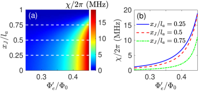
Figure 2: (a) The nonlinear coupling strength $\chi/2\pi$ versus the external flux $\Phi^{\prime}_{e}/\Phi_{0}$ and the position $x_{J}/l_{a}$ of the SQUID. (b) The nonlinear coupling strength $\chi$ versus the external flux $\Phi^{\prime}_{e}/\Phi_{0}$ for $x_{J}/l_{a}=$ 0.25, 0.5 and 0.75, which are the cross-section views of (a) indicated by the three white dashed lines. Other parameters are $2l_{a}=12$ mm, $2l_{b}=\pi\upsilon/(2\omega_{a})$, $L_{0}=4.5\times 10^{-7}$ H/m, $C_{0}=1.8\times 10^{-10}$ F/m, $E_{J}/2\pi=600$ GHz, $E_{C}/2\pi=1$ GHz, $s/(2l_{a})=0.05$, and $b_{2}=0.5b_{1}$.

In Fig. 2(a), we plot the nonlinear coupling strength $\chi$ versus both the external magnetic flux $\Phi^{\prime}_{e}/\Phi_{0}$ and the position $x_{J}/l_{a}$ of the SQUID. When the SQUID is located at the position near the center of CWR-A and the reduced external flux $\Phi^{\prime}_{e}/\Phi_{0}$ approaches 0.45, i.e., around the bottom right corner of Fig. 2(a), a large coupling strength can be obtained. For clarity, in Fig. 2(b), we also show the results for $x_{J}/l_{a}=0.25,0.5$ and $0.75$, corresponding to the three white dashed lines in Fig. 2(a). For $x_{J}/l_{a}=0.25$ and $\Phi^{\prime}_{e}/\Phi_{0}=0.45$, the nonlinear coupling strength is $\chi/2\pi=18$ MHz, approximately three orders of magnitude higher than that achieved in previous studies Moon05 ; Wang15 . Since the frequencies of the CWR-A and CWR-B, $\omega_{a}$ and $\omega_{b}$, are in the microwave domain (a few gigahertz), the condition $\chi\ll\{\omega_{a},\omega_{b}\}$ to make the RWA in Eq. (11) is well satisfied. As shown in Sec. III, a larger nonlinear coupling strength can give rise to an appreciable enhancement of the microwave squeezing in the proposed circuit, which reveals the advantage of our system.

The decay rate of a superconducting CWR is usually smaller than $1\times 2\pi$ MHz Xiang13 . Therefore, the proposed SQC system can reach the strong-coupling regime, i.e., $\chi$ is larger than the decay rates of CWR-A and CWR-B, where the photon blockade, inaccessible in the weak-coupling regime, can be engineered via the quantized-field-driven PDC Zhou2020 . In fact, under the conditions of both $\Phi^{\prime}_{e}\gg\Phi_{b}$ and $E_{J}(\Phi_{e})\gg E_{c}$, an even larger coupling strength $\chi$ can be achieved by further increasing the static magnetic flux $\Phi^{\prime}_{e}$. Thus, our setup also provides the advantage to demonstrate the photon blockade in a SQC system.

III Microwave squeezing enhancement

In this section, we study the performance of our scheme for microwave squeezing. When a microwave field with frequency $\omega_{d}$ drives CWR-B, the interaction Hamiltonian is $H_{d}=\Omega_{d}(b^{{\dagger}}e^{-i\omega_{d}t}+be^{i\omega_{d}t})$, where $\Omega_{d}$ is the drive strength. In the rotating frame with respect to the drive-field frequency $\omega_{d}$, when $\omega_{b}=2\omega_{a}$ and $\omega_{d}=\omega_{b}$, the total Hamiltonian $H=H_{0}+H_{d}$ of the system can be written as

$$H=-\chi(a^{{\dagger}}a^{{\dagger}}b+aab^{{\dagger}})+\Omega_{d}(b^{{\dagger}}+b).$$ (12)

Intuitively, by taking the parametric approximation (i.e., replacing the operators $b$ and $b^{{\dagger}}$ with their expectation values $\beta$ and $\beta^{*}$) and removing the constant terms, the above Hamiltonian can be approximated as Moon05

$$H\approx-(\chi_{\rm eff}a^{{\dagger}}a^{{\dagger}}+\chi_{\rm eff}^{*}aa),$$ (13)

with $\chi_{\rm eff}=\chi\beta$, which is a standard two-photon Hamiltonian for generating the squeezing. To be more precise, here we do not adopt this approximation, but directly harness the Hamiltonian in Eq. (12) to study the microwave squeezing of the proposed system.

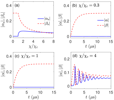
Figure 3: (a) The microwave-field amplitudes $|\alpha_{s}|$ and $|\beta_{s}|$ versus the reduced coupling strength $\chi/\chi_{c}$, calculated using Eqs. (16) and (17). (b)-(d) The time evolution of the microwave-field amplitudes $|\alpha|$ and $|\beta|$, calculated using Eq. (III), where the initial values are $\alpha(t=0)=0.01$ and $\beta(t=0)=0.01i$, with (b) $\chi/\chi_{c}=0.3$, (c) $\chi/\chi_{c}=1$, and (d) $\chi/\chi_{c}=4$. Since the fabrication of the SQUID may reduce the quality factor of CWR-A by one or two orders of magnitude Zhong_2013 , we choose $\kappa_{b}=0.1\kappa_{a}$. Other parameters are $\kappa_{a}/2\pi=2$ MHz and $\Omega_{d}/2\pi=0.03$ MHz.

We assume that the CWR-A and CWR-B interact with their respective thermal reservoirs, which are independent from each other. Via the Heisenberg-Langevin approach Scully97 , the equations of motion for the field operators $a$ and $b$ can be written as

$$\dot{a} =2i\chi a^{{\dagger}}b-\frac{\kappa_{a}}{2}a+F_{a}(t),$$

$$\dot{b} =i\chi aa-i\Omega_{d}-\frac{\kappa_{b}}{2}b+F_{b}(t),$$ (14)

where $\kappa_{a}$ and $\kappa_{b}$ are the decay rates of CWR-A and CWR-B, respectively, while $F_{a}(t)$ and $F_{b}(t)$ are the related noise operators. In order to linearize Eq. (III), we write the operator $a$ $(b)$ as a sum of the expectation value $\alpha$ $(\beta)$ and the fluctuation $\delta a$ $(\delta b)$, i.e., $a=\alpha+\delta a$ and $b=\beta+\delta b$. It follows from Eq. (III) that the expectation values $\alpha$ and $\beta$ satisfy

$$\dot{\alpha} =2i\chi\alpha^{*}\beta-\frac{\kappa_{a}}{2}\alpha,$$

$$\dot{\beta} =i\chi\alpha^{2}-i\Omega_{d}-\frac{\kappa_{b}}{2}\beta.$$ (15)

At the steady state, $\dot{\alpha}=\dot{\beta}=0$. Solving Eq. (III) with $\dot{\alpha}=\dot{\beta}=0$, we obtain two sets of solutions. One set of solutions are

$$\alpha_{s}=0,~{}~{}\beta_{s}=-2i\Omega_{d}/\kappa_{b},$$ (16)

and the other set of solutions are

$$\alpha_{s}=\pm\sqrt{\Omega_{d}(\chi-\chi_{c})}/\chi,~{}~{}\beta_{s}=-i\kappa_{a}/4\chi,$$ (17)

which are steady for $\chi<\chi_{c}$ and $\chi>\chi_{c}$ Wang15 , respectively, with $\chi_{c}=\kappa_{a}\kappa_{b}/(8\Omega_{d})$ being the critical coupling strength. Due to the occurrence of the second-order phase transition, the microwave-field amplitudes in both CWR-A and CWR-B display abrupt changes at $\chi/\chi_{c}=1$, as shown in Fig. 3(a). When $\chi/\chi_{c}<1$, the absolute values $|\alpha_{s}|$ and $|\beta_{s}|$, given by Eq. (16), are constants. However, in the case of $\chi/\chi_{c}>1$, as the reduced coupling strength $\chi/\chi_{c}$ increases, the absolute value $|\alpha_{s}|$, given by Eq. (17), increases from 0 at $\chi/\chi_{c}=1$ to 0.07 around $\chi/\chi_{c}=2$ and then decreases monotonically (blue solid curve), while the absolute value $|\beta_{s}|$, also given by Eq. (17), monotonically decreases with the reduced coupling strength $\chi/\chi_{c}$ (red dashed curve).

To further study the dynamics of the system, we plot the time evolution of the absolute values $|\alpha|$ and $|\beta|$ for various values of the reduced coupling strength $\chi/\chi_{c}$ in Figs. 3(b)-3(d). It can be seen that below the critical coupling strength (i.e., $\chi/\chi_{c}<1$), the microwave field in CWR-A is almost in the ground state with $|\alpha|\approx 0$ at any time $t$, but the microwave-field amplitude $|\beta|$ of CWR-B increases with the time and finally reaches its steady-state value $|\beta_{s}|=0.3$ [see Figs. 3(b) and 3(c)]. By comparing Figs. 3(b) and 3(c), we find that the evolution of $|\alpha|$ ($|\beta|$) remains nearly the same for different values of $\chi/\chi_{c}$, indicating that in the case of $\chi/\chi_{c}<1$, the evolutions are independent of the reduced coupling strength $\chi/\chi_{c}$ and there is no energy exchange between the two resonators. The reason is that the initial state of CWR-A is nearly in its steady state, while the initial state of CWR-B deviates considerably from its steady state. However, when $\chi$ is larger than the critical value $\chi_{c}$ and the initial states of both CWR-A and CWR-B deviate from their steady states, e.g., $\chi/\chi_{c}$=4 in Fig. 3(d), the time evolutions of $|\alpha|$ and $|\beta|$ exhibit obvious oscillations before reaching their steady-state values $|\alpha_{s}|=0.06$ and $|\beta_{s}|=0.08$, and both CWR-A and CWR-B have energy exchange.

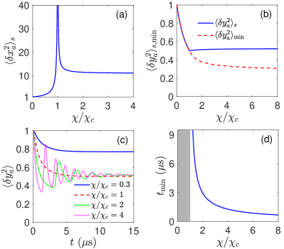
Figure 4: (a) The steady-state variance $\langle\delta x_{a}^{2}\rangle_{s}$ versus the reduced coupling strength $\chi/\chi_{c}$. (b) The steady-state variance $\langle\delta y_{a}^{2}\rangle_{s}$ and the minimum $\langle\delta y_{a}^{2}\rangle_{\rm min}$ versus the reduced coupling strength $\chi/\chi_{c}$. (c) The time evolution of the variance $\langle\delta y_{a}^{2}\rangle$ for $\chi/\chi_{c}=0.3$, 1, 2 and 4. (d) The time $t_{\rm min}$ versus the reduced coupling strength $\chi/\chi_{c}$. Note that no $t_{\rm min}$ exists in the gray region of $\chi/\chi_{c}<1$. Other parameters are the same as in Fig. 3(a).

Below we investigate the microwave squeezing in CWR-A via the variances $\langle\delta x_{a}^{2}\rangle\equiv\langle x_{a}^{2}\rangle-\langle x_{a}\rangle^{2}=\langle(\delta a^{{\dagger}}+\delta a)^{2}\rangle$ and $\langle\delta y_{a}^{2}\rangle\equiv\langle y_{a}^{2}\rangle-\langle y_{a}\rangle^{2}=-\langle(\delta a^{{\dagger}}-\delta a)^{2}\rangle$, where $x_{a}=a^{{\dagger}}+a$ and $y_{a}=i(a^{{\dagger}}-a)$ are the Hermitian amplitude operators. For clarity, here we only give the main results; detailed derivations can be found in Appendix B. At the steady state, the variances $\langle\delta x_{a}^{2}\rangle$ and $\langle\delta y_{a}^{2}\rangle$ can be expressed as

$$\langle\delta x_{a}^{2}\rangle_{s}=\left\{\begin{matrix}\dfrac{\kappa_{a}\kappa_{b}}{\kappa_{a}\kappa_{b}-8\chi\Omega_{d}},&\chi<\chi_{c};\\ 1+\dfrac{\kappa_{a}}{\kappa_{b}}+\dfrac{\kappa_{a}\kappa_{b}}{2(8\chi\Omega_{d}-\kappa_{a}\kappa_{b})},&\chi>\chi_{c},\end{matrix}\right.$$ (18)

and

$$\langle\delta y_{a}^{2}\rangle_{s}=\left\{\begin{matrix}\dfrac{\kappa_{a}\kappa_{b}}{\kappa_{a}\kappa_{b}+8\chi\Omega_{d}},&\chi<\chi_{c};\\ \dfrac{16\chi\Omega_{d}(\kappa_{a}+\kappa_{b})-\kappa_{a}\kappa_{b}^{2}}{16\chi\Omega_{d}(2\kappa_{a}+\kappa_{b})},&\chi>\chi_{c}.\end{matrix}\right.$$ (19)

At the critical point $\chi/\chi_{c}=1$, the variance $\langle\delta y_{a}^{2}\rangle_{s}$ has an abrupt change, while the variance $\langle\delta x_{a}^{2}\rangle_{s}$ is divergent, which is a characteristic of the second-order phase transition Zhu20 . In Figs. 4(a) and 4(b), we plot the steady-state variances $\langle\delta x_{a}^{2}\rangle_{s}$ and $\langle\delta y_{a}^{2}\rangle_{s}$ versus the reduced coupling strength $\chi/\chi_{c}$ (blue solid curves). The steady-state variance $\langle\delta x_{a}^{2}\rangle_{s}$ is always larger than 1, while the conjugate variance $\langle\delta y_{a}^{2}\rangle_{s}$ is smaller than 1. This implies the emergence of microwave squeezing in CWR-A Wang15 ; Moon05 . When $\chi/\chi_{c}<1$, $\langle\delta y_{a}^{2}\rangle_{s}$ decreases monotonically from $1$ to $0.5$, while it increases monotonically from $0.5$ to $0.524$ in the region of $\chi/\chi_{c}>1$, where the optimum steady-state squeezing is $\langle\delta y_{a}^{2}\rangle_{s}=0.5$ around the critical point $\chi/\chi_{c}=1$.

Moreover, we also present the time evolution of the variance $\langle\delta y_{a}^{2}\rangle$ for different values of the reduced coupling strength $\chi/\chi_{c}$ in Fig. 4(c). It can be seen that below the critical coupling strength, the variance $\langle\delta y_{a}^{2}\rangle$ decreases monotonically with time $t$ to its minimum $\langle\delta y_{a}^{2}\rangle_{\rm min}$ ($=\langle\delta y_{a}^{2}\rangle_{s}$), corresponding to the optimum squeezing (cf. the blue solid and red dashed curves). However, when the coupling strength exceeds the critical value $\chi_{c}$, the variance $\langle\delta y_{a}^{2}\rangle$ decreases monotonically with time $t$ to its minimum $\langle\delta y_{a}^{2}\rangle_{\rm min}$ ($<\langle\delta y_{a}^{2}\rangle_{s}$) and then oscillates before reaching the steady-state value $\langle\delta y_{a}^{2}\rangle_{s}$. These dynamical behaviors of the microwave squeezing can be understood using the parametric-approximation Hamiltonian in Eq. (13). Below the critical coupling strength, the effective nonlinear coefficient $|\chi_{\rm eff}|$ ($\propto|\beta|$) increases monotonically with time $t$ [cf. Figs. 3(b) and 3(c)], which is responsible for the monotonic decrease of the variance $\langle\delta y_{a}^{2}\rangle$. When $\chi/\chi_{c}>1$ (i.e., above the critical coupling strength), the oscillatory $|\chi_{\rm eff}|$ ($\propto|\beta|$) results in the oscillating behavior of the variance $\langle\delta y_{a}^{2}\rangle$ [cf. Fig. 3(d)].

In addition, we plot the minimum $\langle\delta y_{a}^{2}\rangle_{\rm min}$ versus the reduced coupling strength $\chi/\chi_{c}$ in Fig. 4(b) (the red dashed curve) as well as the time $t_{\rm min}$ (for reaching $\langle\delta y_{a}^{2}\rangle_{\rm min}$) versus $\chi/\chi_{c}$ in Fig. 4(d). Note that $\langle\delta y_{a}^{2}\rangle$ decreases monotonically with time $t$ in the region of $\chi/\chi_{c}<1$ and the time $t_{\rm min}$ does not exist [see the gray region in Fig. 4(d)]. Because both $\langle\delta y_{a}^{2}\rangle_{\rm min}$ and $t_{\rm min}$ versus $\chi/\chi_{c}$ decrease monotonically, a larger coupling strength can yield more appreciable and faster squeezing. This promises a considerable enhancement of the microwave squeezing via the quantized-field-driven PDC in our proposed circuit, where the PDC coefficient is strengthened by three orders of magnitude, from tens of kilohertz in Ref. Moon05 ; Wang15 to tens of megahertz in the present work. When generating the squeezing, the amplitude of the quantized microwave field in CWR-B is on the order of $\kappa_{a}/\chi$ [cf. Eqs. (16)-(17) and Fig. 3], smaller than 1 because the proposed system is in the strong-coupling regime with $\{\kappa_{a},\kappa_{b}\}_{\rm max}<\chi$. This reveals that microwave squeezing is implemented in the CWR-A, with CWR-B in the quantum limit of single photon.

The above results are obtained at zero temperature, i.e., we take $n_{a}=n_{b}=0$ in the correlation functions $\langle F_{q}^{{\dagger}}(t)F_{q}(t^{\prime})\rangle=n_{q}\kappa_{q}\delta(t-t^{\prime})$ and $\langle F_{q}(t)F_{q}^{{\dagger}}(t^{\prime})\rangle=(n_{q}+1)\kappa_{q}\delta(t-t^{\prime})$ with $q=a,b$ (cf. Appendix B), where $n_{a}$ and $n_{b}$ are the numbers of thermal average photons in CWR-A and CWR-B. In experiments, the SQCs operate at milli-Kelvin temperatures Gu17 , and the typical frequencies of CWRs are a few gigahertz. If we choose $\omega_{a}/2\pi=3.5$ GHz and $\omega_{b}=2\omega_{a}$, the numbers of thermal average photons in CWR-A and CWR-B are about $n_{a}=2.2\times 10^{-4}$ and $n_{b}=5\times 10^{-8}$ at 20 mK ($n_{a}=1.5\times 10^{-2}$ and $n_{b}=2.2\times 10^{-4}$ even at 40 mK), respectively. Therefore, it is reasonable to neglect the temperature effect.

Note that when replacing CWR-B with a transmission line, the system is reduced to a flux-driven JPA, which is a standard device for creating microwave squeezing in the SQCs Gu17 . For the JPA driven by a classical field via the transmission line, the Hamiltonian of the system can be written as Zhong_2013 $H_{\rm JPA}=i\Omega_{d}(a^{{\dagger}2}-a^{2})$. For simplicity, we use the same symbol $\Omega_{d}$ in both cases. When $\Omega_{d}/\kappa_{a}<0.25$, the steady-state value coincides the minimum of the variance $\langle\delta y_{a}^{2}\rangle$, i.e., $\langle\delta y_{a}^{2}\rangle_{s}=\langle\delta y_{a}^{2}\rangle_{\rm min}=\kappa_{a}/(\kappa_{a}+4\Omega_{d})$ Scully97 , which decrease monotonically with the drive strength $\Omega_{d}/\kappa_{a}$, but the JPA becomes unstable for $\Omega_{d}/\kappa_{a}>0.25$. Since the JPA can become unstable around the critical point $\Omega_{d}/\kappa_{a}=0.25$, $\langle\delta y_{a}^{2}\rangle_{s}=\langle\delta y_{a}^{2}\rangle_{\rm min}=0.5$ is experimentally inaccessible. On the contrary, our proposed system is stable around the critical point and the optimum steady-state squeezing $\langle\delta y_{a}^{2}\rangle_{s}=0.5$ can be experimentally achievable [cf. Fig. 4(b)]; note that Fig. 4(b) is plotted by fixing the critical coupling strength $\chi_{c}$ (related to the drive strength $\Omega_{d}$) and varying the coupling strength $\chi$. When fixing $\chi$ and varying $\chi_{c}$, a similar figure can be obtained. Moreover, the proposed system is stable above the critical drive strength, where the minimum $\langle\delta y_{a}^{2}\rangle_{\rm min}$ is smaller than 0.5, which is also beyond the JPA [cf. Fig. 4(b)].

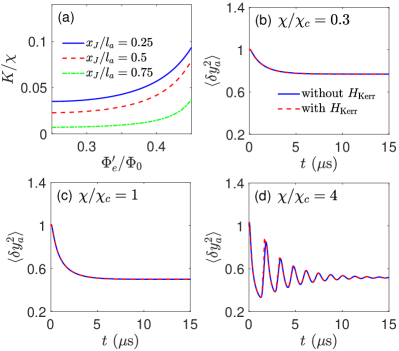
Figure 5: (a) The ratio $K/\chi$ versus the external flux $\Phi^{\prime}_{e}/\Phi_{0}$ for $x_{J}/l_{a}=$ 0.25, 0.5 and 0.75. Other parameters are the same as in Fig. 2. (b)-(d) The time evolution of the variance $\langle\delta y_{a}^{2}\rangle$ in the two cases without and with the Kerr term, respectively, where the reduced coupling strength and the corresponding Kerr coefficient are (b) $\chi/\chi_{c}=0.3$, $K/\chi=0.008$, (c) $\chi/\chi_{c}=1$, $K/\chi=0.013$, and (d) $\chi/\chi_{c}=4$, $K/\chi=0.027$. Here the SQUID are located at $x_{J}/l_{a}=0.75$, and the different values of $\chi$ and $K$ in (b)-(d) correspond to different external flux $\Phi^{\prime}_{e}$ [cf. green dashed-dotted curve in (a)]. Other parameters are the same as in Fig. 3(a).

IV Discussions and conclusions

In the above study, the higher-order nonlinear effect related to $\mathcal{L}_{S}^{(4)}$ is not considered. Below we show that this approximation is reasonable. With the relation in Eq. (II.1), we can obtain the Kerr Hamiltonian $H_{\rm Kerr}=-\mathcal{L}_{S}^{(4)}=-Ka^{{\dagger}}aa^{{\dagger}}a$ under the RWA, where the Kerr coefficient is

$$K=\frac{1}{24L_{J}}\bigg{(}\frac{2\pi}{\Phi_{0}}\bigg{)}^{2}\bigg{(}\frac{\hbar\Delta_{1}^{2}}{2C_{\Sigma}{\omega_{a}}}\bigg{)}^{2}.$$ (20)

Figure 5(a) displays the ratio of the Kerr coefficient $K$ to the coupling strength $\chi$ versus the external flux $\Phi^{\prime}_{e}/\Phi_{0}$ at different positions $x_{J}/l_{a}$ of the SQUID. The corresponding $\chi$ versus $\Phi^{\prime}_{e}/\Phi_{0}$ can be found in Fig. 2(b). For different values of $x_{J}/l_{a}$, the ratio $K/\chi$ increases monotonically with $\Phi^{\prime}_{e}/\Phi_{0}$. Also, for a fixed external flux $\Phi^{\prime}_{e}/\Phi_{0}$, the ratio $K/\chi$ decreases when increasing $x_{J}/l_{a}$. Based on the results in Figs. 5(a) and 2(b), it is vital to choose appropriate $\Phi^{\prime}_{e}/\Phi_{0}$ and $x_{J}/l_{a}$ to have a stronger coupling strength $\chi$ but still keep the ratio $K/\chi$ reasonably small.

Figures 5(b)-5(d) present the time evolution of the variance $\langle\delta y_{a}^{2}\rangle$ in the two cases without and with the Kerr term for different coupling strength $\chi/\chi_{c}$ (see Appendix B for the detailed calculations). Obviously, the variance $\langle\delta y_{a}^{2}\rangle$ shows minor difference in these two cases for various values of $\chi/\chi_{c}$ (cf. the blue solid and red dashed curves). Therefore, it is reasonable to neglect the effect of the higher-order nonlinearities in our scheme. Moreover, only the microwave squeezing in CWR-A is investigated above. In fact, CWR-B can also exhibit the squeezing effect above the critical point (i.e., $\chi/\chi_{c}>1$), but weaker than CWR-A (see Appendix C).

There are also other theoretical proposals for producing microwave squeezing using, e.g., superconducting resonant tank circuits Zagoskin08 , circuit quantum electrodynamical systems Benlloch14 ; Elliott15 and cavity magnomechanical systems Li21 , but those schemes have not been explored experimentally. Different from those schemes, the JPA is widely studied in the experiment and our proposal provides an improved scheme modified from the flux-driven JPA. With the existing technologies, our proposed circuit can be easily fabricated in the experiment Baust15 . Besides generating the squeezing, our scheme may have other potential applications in quantum technologies. For example, in our scheme, the nonlinear interaction of quantized-field-driven PDC can be achieved in the strong-coupling regime, because the typical decay rate of the CWR is smaller than $1\times 2\pi$ MHz Xiang13 and the strong-coupling condition $\chi>\{\kappa_{a},\kappa_{b}\}_{\rm max}$ can be well satisfied. With this strong-coupling quantized-field-driven PDC, the photon blockade becomes achievable Zhou2020 , while it is inaccessible in the weak-coupling regime.

In conclusion, we have shown that the microwave squeezing can be considerably enhanced by designing a SQC, with two CWRs coupled via a SQUID embedded in one of the CWRs. In contrast to the flux-driven JPA Zhong_2013 , optimum steady-state squeezing is experimentally accessible around the critical point and stronger transient squeezing is achievable above the critical drive strength in our scheme. Also, compared with the existing schemes of generating microwave squeezing via PDC Moon05 ; Wang15 , our proposed SQC system can increase the nonlinear coupling strength by three orders of magnitude (i.e., from tens of kilohertz to tens of megahertz). This promises an appreciable enhancement of the microwave squeezing in the resonator.

Appendix A Normal modes of CWR-A

With the Lagrangian $\mathcal{L}^{\prime}_{a}$ of bare CWR-A in Eq. (1) and the linear term $\mathcal{L}_{S}^{(2)}$ of the Lagrangian of the SQUID in Eq. (II.1), we can obtain the total linear Lagrangian $\mathcal{L}_{a}=\mathcal{L}^{\prime}_{a}+\mathcal{L}_{S}^{(2)}$,

$$\mathcal{L}_{a} = \int_{-l_{a}}^{l_{a}}\bigg{[}\frac{C_{0}}{2}\dot{\Phi}^{2}(x,t)-\frac{[\partial_{x}\Phi(x,t)]^{2}}{2L_{0}}\bigg{]}dx$$ (21)

$$+\frac{C_{J}}{2}\dot{\delta}^{2}-\frac{\delta^{2}}{2L_{J}}.$$

According to the Euler-Lagrange equation of motion, the flux field $\Phi(x,t)$ is found to obey the wave equation

$$\ddot{\Phi}(x,t)-\upsilon^{2}\partial_{xx}\Phi(x,t)=0,$$ (22)

with the velocity $\upsilon=1/\sqrt{C_{0}L_{0}}$. By separating the variables, we write the solution in the form of

$$\Phi(x,t)=\sum_{m}\phi_{m}(t)\mu_{m}(x),$$ (23)

where $\phi_{m}$ is the flux amplitude of the $m$th mode of CWR-A and $\mu_{m}(x)$ is the corresponding spatial mode function. Substituting Eq. (23) into Eq. (22), we obtain two independent ordinary differential equations,

$$~{}~{}~{}~{}~{}~{}\ddot{\phi}_{m}(t)+\omega_{m}^{2}\phi_{m}(t) =0,$$

$$\partial_{xx}\mu_{m}(x)+k_{m}^{2}\mu_{m}(x) =0,$$ (24)

with the wave vector $k_{m}$ and the mode frequency $\omega_{m}=k_{m}\upsilon$.

To satisfy the boundary conditions in Eq. (3) and the conditions in Eq. (4) for the point $x=x_{J}$, the general solution of the spatial mode function $\mu_{m}(x)$ takes the form

$$\mu_{m}(x)=A_{m}\bigg{\{}\begin{matrix}\sin[k_{m}(x+l_{a})-\varphi_{0}],&-l_{a}\leq x\leq x_{J}^{-},\\ B_{m}\sin[k_{m}(x-l_{a})+\varphi_{0}],&x_{J}^{+}\leq x\leq l_{a}.\end{matrix}~{}~{}~{}~{}~{}$$ (25)

From Eq. (3), the phase $\varphi_{0}=\pi/2$ can be obtained. By substituting the spatial mode function in Eq. (25) into Eq. (4), we get the expression for the relative amplitudes $B_{m}$,

$$B_{m}=\frac{\cos[k_{m}(x_{J}+l_{a})-\varphi_{0}]}{\cos[k_{m}(x_{J}-l_{a})+\varphi_{0}]},$$ (26)

and the transcendental equation for the wave vectors $k_{m}$,

$$\bigg{(}\tan[k_{m}(x_{J}-l_{a})+\varphi_{0}]-\tan[k_{m}(x_{J}+l_{a})-\varphi_{0}]\bigg{)}$$

$$\times\bigg{[}-(k_{m}l_{a})^{2}\frac{C_{J}}{C_{0}l_{a}}+\frac{L_{0}l_{a}}{L_{J}}\bigg{]}=k_{m}l_{a},$$ (27)

which can be numerically solved. The normalization constants $A_{m}$ can be fixed with the inner product relation Goldstein80

$$\langle\mu_{m}\cdot\mu_{n}\rangle \equiv \int_{-l_{a}}^{l_{a}}dxC_{0}\mu_{m}(x)\mu_{n}(x)+C_{J}\Delta_{m}\Delta_{n}$$ (28)

$$= C_{\Sigma}\delta_{mn},$$

where $\Delta_{m}=\mu_{m}(x_{J}^{+})-\mu_{m}(x_{J}^{-})$ is the mode-amplitude difference across the SQUID, and $C_{\Sigma}=2C_{0}l_{a}+C_{J}$ is the total capacitance. In addition, from Eqs. (A) and (28), the inner product of the envelope derivatives are found to obey a similar orthonormality condition,

$$\langle\partial_{x}\mu_{m}\cdot\partial_{x}\mu_{n}\rangle \equiv \int_{-l_{a}}^{l_{a}}dx\frac{1}{L_{0}}\partial_{x}\mu_{m}(x)\partial_{x}\mu_{n}(x)+\frac{1}{L_{J}}\Delta_{m}\Delta_{n}$$ (29)

$$= \frac{\delta_{mn}}{L_{m}},$$

where $L_{m}$ defined by $1/L_{m}=C_{\Sigma}\omega_{m}^{2}$ is the effective inductance of the $m$th mode. Substituting the normal-mode expansion in Eq. (23) into Eq. (21) and then performing spatial integration, we can write the Lagrangian $\mathcal{L}_{a}$ in the form of a set of harmonic oscillators,

$$\mathcal{L}_{a}=\sum_{m}\left[\frac{1}{2}C_{\Sigma}\dot{\phi}_{m}^{2}-\frac{\phi_{m}^{2}}{2L_{m}}\right],$$ (30)

where the relations in Eqs. (28) and (29) are used.

Appendix B Dynamical equations of CWR-A and CWR-B

When including the higher-order nonlinear effect of the SQUID, which corresponds to adding a Kerr term $-Ka^{{\dagger}}aa^{{\dagger}}a$ to the Hamiltonian $H$ in Eq. (12), the total Hamiltonian of the system becomes

$$H_{\rm tot}=-\chi(a^{{\dagger}}a^{{\dagger}}b+aab^{{\dagger}})-Ka^{{\dagger}}aa^{{\dagger}}a+\Omega_{d}(b^{{\dagger}}+b).$$ (31)

To study the microwave squeezing in the system, we define the variances $\langle\delta x_{o}^{2}\rangle\equiv\langle x_{o}^{2}\rangle-\langle x_{o}\rangle^{2}=\langle(\delta o^{{\dagger}}+\delta o)^{2}\rangle$ and $\langle\delta y_{o}^{2}\rangle\equiv\langle y_{o}^{2}\rangle-\langle y_{o}\rangle^{2}=-\langle(\delta o^{{\dagger}}-\delta o)^{2}\rangle$, with $o=a,~{}b$, where the Hermitian amplitude operators are given by $x_{o}=(o^{{\dagger}}+o)$ and $y_{o}=i(o^{{\dagger}}-o)$. Below we derive the variances $\langle\delta x_{a}^{2}\rangle$ and $\langle\delta y_{a}^{2}\rangle$ for the microwave field in CWR-A, as well as the variances $\langle\delta x_{b}^{2}\rangle$ and $\langle\delta y_{b}^{2}\rangle$ for the microwave field in CWR-B.

With the Hamiltonian in Eq. (31), the dynamics of the proposed system is governed by the following Heisenberg-Langevin equations:

$$\dot{a} =2i\chi a^{{\dagger}}b+iK(aa^{{\dagger}}a+a^{{\dagger}}aa)-\frac{\kappa_{a}}{2}a+F_{a}(t),$$

$$\dot{b} =i\chi aa-i\Omega_{d}-\frac{\kappa_{b}}{2}b+F_{b}(t),$$ (32)

where $\kappa_{a}$ and $\kappa_{b}$ are the decay rates of the microwave fields in CWR-A and CWR-B, respectively. Here $F_{a}(t)$ and $F_{b}(t)$ are the corresponding input noise operators, which satisfy $\langle F_{q}(t)\rangle=0$, $\langle F_{q}(t)F_{q}(t^{\prime})\rangle=\langle F_{q}^{{\dagger}}(t)F_{q}^{{\dagger}}(t^{\prime})\rangle=0$, $\langle F_{q}^{{\dagger}}(t)F_{q}(t^{\prime})\rangle=n_{q}\kappa_{q}\delta(t-t^{\prime})$, and $\langle F_{q}(t)F_{q}^{{\dagger}}(t^{\prime})\rangle=(n_{q}+1)\kappa_{q}\delta(t-t^{\prime})$, with $q=a,b$, where $n_{a}$ and $n_{b}$ are the numbers of thermal average photons in CWR-A and CWR-B. Due to the fact that the SQCs operate at milli-Kelvin temperatures Gu17 , it is reasonable to ignore the temperature effect and take $n_{a}=n_{b}=0$. Following the procedures in Refs. Wang15 ; Marshall90 , if we write the operators $a$ and $b$ as $a=\alpha+\delta a$ and $b=\beta+\delta b$, with $\alpha$ $(\beta)$ being the expectation value and $\delta a$ $(\delta b)$ the fluctuation, it follows from Eq. (B) that the average values $\alpha$ and $\beta$ satisfy

$$\dot{\alpha} =2i\chi\alpha^{*}\beta+2iK|\alpha|^{2}\alpha-\frac{\kappa_{a}}{2}\alpha,$$

$$\dot{\beta} =i\chi\alpha^{2}-i\Omega_{d}-\frac{\kappa_{b}}{2}\beta,$$ (33)

and the fluctuation operators $\delta a$ and $\delta b$ obey

$$\frac{d}{dt}\delta a = 2i\chi\alpha^{*}\delta b+2(i\chi\beta+iK\alpha^{2})\delta a^{{\dagger}}$$

$$+(4iK|\alpha|^{2}-\kappa_{a}/2)\delta a+F_{a}(t),$$

$$\frac{d}{dt}\delta b = 2i\chi\alpha\delta a-\frac{\kappa_{b}}{2}\delta b+F_{b}(t),$$ (34)

where the high-order terms of the fluctuations have been neglected. In the special case without the Kerr effect (i.e., $K=0$), the linearization procedure in Eq. (B) gives the correct results both below and above the critical point, as discussed in Refs. Wang15 ; Marshall90 . In our scheme, the Kerr coefficient is much weaker than the coupling strength [cf. Fig. 5(a) and related discussions], and the Kerr effect can be regarded as a perturbation Boutin17 . Thus, the linearized approximation used in Eq. (B) is well justified.

To investigate the variances of the proposed system, we define the correlation parameters $A_{1}=\langle\delta a^{2}\rangle$, $A_{2}=\langle\delta a^{{\dagger}}\delta a\rangle+\langle\delta a\delta a^{{\dagger}}\rangle$, and $A_{3}=\langle\delta a^{{\dagger}2}\rangle$ for CWR-A, which are related to the two-operator fluctuations. Using Eq. (B), we obtain the equations of motion for $A_{1}$, $A_{2}$ and $A_{3}$,

$$\dot{A}_{1} = 4i\chi\alpha^{*}C_{1}+2(i\chi\beta+iK\alpha^{2})A_{2}+2(4iK|\alpha|^{2}-\kappa_{a}/2)A_{1}$$

$$+\langle\delta aF_{a}(t)+F_{a}(t)\delta a\rangle,$$

$$\dot{A}_{2} = \left[4i\chi\alpha^{*}C_{2}+4(i\chi\beta+iK\alpha^{2})A_{3}\right.$$

$$\left.+\langle\delta a^{{\dagger}}F_{a}(t)+F_{a}(t)\delta a^{{\dagger}}\rangle+h.c.\right]-\kappa_{a}A_{2},$$

$$\dot{A}_{3} = -4i\chi\alpha C_{1}^{*}-2(i\chi\beta^{*}+iK\alpha^{*2})A_{2}-2(4iK|\alpha|^{2}+\kappa_{a}/2)A_{3}$$ (35)

$$+\langle\delta a^{{\dagger}}F^{{\dagger}}_{a}(t)+F^{{\dagger}}_{a}(t)\delta a^{{\dagger}}\rangle,$$

where $C_{1}=\langle\delta a\delta b\rangle$ and $C_{2}=\langle\delta a^{{\dagger}}\delta b\rangle$ are the cross-correlation parameters for both CWR-A and CWR-B. Note that all correlation functions involving the noise operators in Eq. (B) are zero, except for $\langle F_{a}(t)a^{{\dagger}}\rangle=\langle aF_{a}^{{\dagger}}(t)\rangle=\kappa_{a}/2$ Scully97 . Therefore, Eq. (B) reduces to

$$\dot{A}_{1} =4i\chi\alpha^{*}C_{1}+2(i\chi\beta+iK\alpha^{2})A_{2}+2(4iK|\alpha|^{2}-\kappa_{a}/2)A_{1},$$

$$\dot{A}_{2} =[4i\chi\alpha^{*}C_{2}+4(i\chi\beta+iK\alpha^{2})A_{3}+h.c.]-\kappa_{a}A_{2}+\kappa_{a},$$

$$\dot{A}_{3} =-4i\chi\alpha C_{1}^{*}-2(i\chi\beta^{*}+iK\alpha^{*2})A_{2}-2(4iK|\alpha|^{2}+\kappa_{a}/2)A_{3}.$$ (36)

With similar procedures, the equations of motion for the cross-correlation parameters $C_{1}$ and $C_{2}$ are given by

$$\dot{C}_{1} = 2i\chi\alpha^{*}B_{1}+2i\chi\alpha A_{1}+2(i\chi\beta+iK\alpha^{2})C_{2}$$

$$+(4iK|\alpha|^{2}-\kappa_{a}/2-\kappa_{b}/2)C_{1},$$

$$\dot{C}_{2} = -i\chi\alpha(B_{2}-1)+i\chi\alpha(A_{2}-1)-2(i\chi\beta^{*}+iK\alpha^{*2})C_{1}$$ (37)

$$-(4iK|\alpha|^{2}+\kappa_{a}/2+\kappa_{b}/2)C_{2},$$

where the correlation parameters $B_{1}=\langle\delta b^{2}\rangle$, $B_{2}=\langle\delta b^{{\dagger}}\delta b\rangle+\langle\delta b\delta b^{{\dagger}}\rangle$ and $B_{3}=\langle\delta b^{{\dagger}2}\rangle$ for CWR-B satisfy

$$\dot{B}_{1} =4i\chi\alpha C_{1}-\kappa_{b}B_{1},$$

$$\dot{B}_{2} =4i\chi\alpha C_{2}^{*}-4i\chi\alpha^{*}C_{2}-\kappa_{b}B_{2}+\kappa_{b},$$

$$\dot{B}_{3} =-4i\chi\alpha^{*}C_{1}^{*}-\kappa_{b}B_{3}.$$ (38)

Here we assume that the noise operators $F_{a}(t)$ and $F_{b}(t)$ are independent for the two resonators, i.e., $\langle F_{a}(t)F_{b}(t^{\prime})\rangle=\langle F^{{\dagger}}_{a}(t)F^{{\dagger}}_{b}(t^{\prime})\rangle=\langle F^{{\dagger}}_{a}(t)F_{b}(t^{\prime})\rangle=\langle F_{a}(t)F^{{\dagger}}_{b}(t^{\prime})\rangle=0$, under which $\langle aF_{b}(t)\rangle=\langle a^{{\dagger}}F_{b}(t)\rangle=\langle bF_{a}(t)\rangle=\langle bF^{{\dagger}}_{a}(t)\rangle=0$. Obviously, the variances $\langle\delta x_{a}^{2}\rangle$, $\langle\delta y_{a}^{2}\rangle$, $\langle\delta x_{b}^{2}\rangle$ and $\langle\delta y_{b}^{2}\rangle$ can be expressed using the correlation parameters in Eqs. (B)-(B). With Eqs. (B) and (B)-(B), we show the time evolution of the microwave-field amplitudes and the variances in Figs. 3-6, where the initial states in CWR-A and CWR-B are assumed to be coherent states $|\alpha_{0}=0.01\rangle$ and $|\beta_{0}=0.01i\rangle$, respectively, which correspond to $\alpha(t=0)=0.01$, $\beta(t=0)=0.01i$, $A_{1}(t=0)=A_{3}(t=0)=B_{1}(t=0)=B_{3}(t=0)=C_{1}(t=0)=C_{2}(t=0)=0$, and $A_{2}(t=0)=B_{2}(t=0)=1$.

In addition to the dynamical behaviors, we are also interested in the steady-state behaviors of the proposed SQC system. Without the Kerr effect (i.e., $K=0$), Eq. (B) is reduced to Eq. (III), and the corresponding steady-state amplitudes $\alpha_{s}$ and $\beta_{s}$, which satisfy $\alpha_{s}=\alpha_{s}^{*}$ and $\beta_{s}=-\beta_{s}^{*}$, are given in Eqs. (16) and (17). Here we assume that the Rabi frequency $\Omega_{d}$ is real. Using Eqs. (B)-(B) and also with $\alpha=\alpha_{s}=\alpha_{s}^{*}$ and $\beta=\beta_{s}=-\beta_{s}^{*}$, we obtain the dynamical equations of the variances,

$$\frac{d}{dt}\langle\delta x_{a}^{2}\rangle =-4\chi\alpha_{s}\langle\delta x_{a}\delta y_{b}\rangle+(4i\chi\beta_{s}-\kappa_{a})\langle\delta x_{a}^{2}\rangle+\kappa_{a},$$

$$\frac{d}{dt}\langle\delta x_{a}\delta y_{b}\rangle =2\chi\alpha_{s}\langle\delta x_{a}^{2}-\delta y_{b}^{2}\rangle+\left(2i\chi\beta_{s}-\frac{\kappa_{a}+\kappa_{b}}{2}\right)\langle\delta x_{a}\delta y_{b}\rangle,$$

$$\frac{d}{dt}\langle\delta y_{b}^{2}\rangle =4\chi\alpha_{s}\langle\delta x_{a}\delta y_{b}\rangle-\kappa_{b}\langle\delta y_{b}^{2}\rangle+\kappa_{b},$$ (39)

and

$$\frac{d}{dt}\langle\delta y_{a}^{2}\rangle =4\chi\alpha_{s}\langle\delta y_{a}\delta x_{b}\rangle-(4i\chi\beta_{s}+\kappa_{a})\langle\delta y_{a}^{2}\rangle+\kappa_{a},$$

$$\frac{d}{dt}\langle\delta y_{a}\delta x_{b}\rangle =-2\chi\alpha_{s}\langle\delta y_{a}^{2}-\delta x_{b}^{2}\rangle-\left(2i\chi\beta_{s}+\frac{\kappa_{a}+\kappa_{b}}{2}\right)\langle\delta y_{a}\delta x_{b}\rangle,$$

$$\frac{d}{dt}\langle\delta x_{b}^{2}\rangle =-4\chi\alpha_{s}\langle\delta y_{a}\delta x_{b}\rangle-\kappa_{b}\langle\delta x_{b}^{2}\rangle+\kappa_{b}.$$ (40)

Here Eqs. (B) and (B) are valid in the limit $t\rightarrow+\infty$. At the steady states, the steady-state variances $\langle\delta x_{a}^{2}\rangle_{s}$, $\langle\delta y_{a}^{2}\rangle_{s}$, $\langle\delta x_{b}^{2}\rangle_{s}$ and $\langle\delta y_{b}^{2}\rangle_{s}$, as given in Eqs. (18), (19), (41) and (42), can be derived by solving Eqs. (B) and (B) with $d\langle\delta x_{a}^{2}\rangle/dt=d\langle\delta x_{a}\delta y_{b}\rangle/dt=d\langle\delta y_{b}^{2}\rangle/dt=d\langle\delta y_{a}^{2}\rangle/dt=d\langle\delta y_{a}\delta x_{b}\rangle/dt=d\langle\delta x_{b}^{2}\rangle/dt=0$.

Figure 6: (a) The steady-state variances $\langle\delta x_{b}^{2}\rangle_{s}$ and $\langle\delta y_{b}^{2}\rangle_{s}$ versus the reduced coupling strength $\chi/\chi_{c}$. (b) The time evolution of the variance $\langle\delta x_{b}^{2}\rangle$ for $\chi/\chi_{c}=0.3$, 1, 2 and 4. Other parameters are the same as in Fig. 3(a).

Appendix C Microwave squeezing in CWR-B

In Sec. III, we have studied the microwave squeezing in CWR-A. Here we further show the microwave squeezing in CWR-B. At the steady state, the variances $\langle\delta x_{b}^{2}\rangle$ and $\langle\delta y_{b}^{2}\rangle$ are obtained as (see Appendix B)

$$\langle\delta x_{b}^{2}\rangle_{s}=\left\{\begin{matrix}1,&\chi<\chi_{c};\\ \dfrac{8\chi\Omega_{d}(\kappa_{a}+\kappa_{b})+\kappa_{a}^{2}\kappa_{b}}{8\chi\Omega_{d}(2\kappa_{a}+\kappa_{b})},&\chi>\chi_{c},\end{matrix}\right.$$ (41)

and

$$\langle\delta y_{b}^{2}\rangle_{s}=\left\{\begin{matrix}1,&\chi<\chi_{c};\\ (\kappa_{a}+\kappa_{b})/\kappa_{b},&\chi>\chi_{c}.\end{matrix}\right.$$ (42)

When $\chi<\chi_{c}$ (i.e., below the critical point), no microwave squeezing occurs in CWR-B, because $\langle\delta x_{b}^{2}\rangle_{s}=\langle\delta y_{b}^{2}\rangle_{s}=1$. However, when the coupling strength $\chi$ is larger than the critical value $\chi_{c}$, $\langle\delta x_{b}^{2}\rangle_{s}<1$ and $\langle\delta y_{b}^{2}\rangle_{s}>1$ [cf. Fig. 6(a)]. In this region, microwave squeezing can occur in CWR-B.

Compared with the steady-state squeezing in CWR-A, the squeezing effect in CWR-B is weaker (i.e., $\langle\delta x_{b}^{2}\rangle_{s}>\langle\delta y_{a}^{2}\rangle_{s}$) for a finite coupling strength $\chi$ [cf. Figs. 6(a) and 4(b)]. In the limit $\chi/\chi_{c}\rightarrow+\infty$, the two resonators have the same squeezing effect with $\langle\delta y_{a}^{2}\rangle_{s}=\langle\delta x_{b}^{2}\rangle_{s}=0.524$. To further study the squeezing in CWR-B, we plot the time evolution of the variance $\langle\delta x_{b}^{2}\rangle$ for different values of the reduced coupling strength $\chi/\chi_{c}$ in Fig. 6(b) (the related calculation details can be found in Appendix B). Below the critical coupling strength, i.e., $\chi/\chi_{c}<1$, no microwave squeezing occurs in CWR-B (see the blue solid and red dashed curves). While above the critical coupling strength, i.e., $\chi/\chi_{c}>1$, microwave squeezing occurs in CWR-B (see the green dashed-dotted and magenta dotted curves). By comparing Figs. 6(b) and  4(c), we find that for a given coupling strength $\chi$, CWR-A exhibits a stronger squeezing effect than CWR-B.

References

- (1) D. F. Walls, Squeezed states of light, Nature 306(5939), 141-146 (1983).
- (2) R. E. Slusher, L. W. Hollberg, B. Yurke, J. C. Mertz, and J. F. Valley, Observation of Squeezed States Generated by Four-Wave Mixing in an Optical Cavity, Phys. Rev. Lett. 55(22), 2409-2412 (1985).
- (3) L.-A. Wu, H. J. Kimble, J. L. Hall, and H. Wu, Generation of Squeezed States by Parametric Down Conversion, Phys. Rev. Lett. 57(20), 2520-2523 (1986).
- (4) N. Otterstrom, R. C. Pooser, and B. J. Lawrie, Nonlinear optical magnetometry with accessible in situ optical squeezing, Opt. Lett. 39(22), 6533-6536 (2014).
- (5) I. Kruse, K. Lange, J. Peise, B. Lücke, L. Pezzè, J. Arlt, W. Ertmer, C. Lisdat, L. Santos, A. Smerzi, and C. Klempt, Improvement of an Atomic Clock using Squeezed Vacuum, Phys. Rev. Lett. 117(14), 143004 (2016).
- (6) M. Malnou, D. A. Palken, B. M. Brubaker, L. R. Vale, G. C. Hilton, and K. W. Lehnert, Squeezed Vacuum Used to Accelerate the Search for a Weak Classical Signal, Phys. Rev. X 9(2), 021023 (2019).
- (7) R. García-Patrón, and N. J. Cerf, Continuous-Variable Quantum Key Distribution Protocols Over Noisy Channels, Phys. Rev. Lett. 102(13), 130501 (2009).
- (8) P. Wang, X. Wang, and Y. Li, Continuous-variable measurement-device-independent quantum key distribution using modulated squeezed states and optical amplifiers, Phys. Rev. A 99(4), 042309 (2019).
- (9) X.-Y. Lü, Y. Wu, J. R. Johansson, H. Jing, J. Zhang, and F. Nori, Squeezed Optomechanics with Phase-Matched Amplification and Dissipation, Phys. Rev. Lett. 114(9), 093602 (2015).
- (10) S. Zeytinoğlu, A. İmamoğlu, and S. Huber, Engineering Matter Interactions Using Squeezed Vacuum, Phys. Rev. X 7(2), 021041 (2017).
- (11) W. Qin, A. Miranowicz, P.-B. Li, X.-Y. Lü, J. Q. You, and F. Nori, Exponentially Enhanced Light-Matter Interaction, Cooperativities, and Steady-State Entanglement Using Parametric Amplification, Phys. Rev. Lett. 120(9), 093601 (2018).
- (12) J. Klaers, S. Faelt, A. Imamoglu, and E. Togan, Squeezed Thermal Reservoirs as a Resource for a Nanomechanical Engine beyond the Carnot Limit, Phys. Rev. X 7(3), 031044 (2017).
- (13) J. Wang, J. He, and Y. Ma, Finite-time performance of a quantum heat engine with a squeezed thermal bath, Phys. Rev. E 100(5), 052126 (2019).
- (14) C. Fabre, M. Pinard, S. Bourzeix, A. Heidmann, E. Giacobino, and S. Reynaud, Quantum-noise reduction using a cavity with a movable mirror, Phys. Rev. A 49(2), 1337 C1343 (1994).
- (15) Y. Xiao, Y. F. Yu, and Z. M. Zhang, Controllable optomechanically induced transparency and ponderomotive squeezing in an optomechanical system assisted by an atomic ensemble, Opt. express 22(15), 17979 C17989 (2014).
- (16) Z. C. Zhang, Y. P. Wang, Y. F. Yu, and Z. M. Zhang, Quantum squeezing in a modulated optomechanical system, Opt. express 26(9), 11915-11927 (2018).
- (17) D. F. Walls and G. J. Milburn, Quantum Optics (Springer, 1994).
- (18) M. H. Devoret and R. J. Schoelkopf, Superconducting Circuits for Quantum Information: An Outlook, Science 339(6124), 1169-1174 (2013).
- (19) J. Q. You and F. Nori, Atomic physics and quantum optics using superconducting circuits, Nature 474(7353), 589-597 (2011).
- (20) G. Wendin, Quantum information processing with superconducting circuits: a review, Rep. Prog. Phys. 80(10), 106001 (2017).
- (21) S. Kwon, A. Tomonaga, G. L. Bhai, S. J. Devitt, and J. S. Tsai, Gate-based superconducting quantum computing, J. Appl. Phys. 129, 041102 (2021).
- (22) H.-C. Li, G.-Q. Ge, and H.-Y. Zhang, Dressed-state realization of the transition from electromagnetically induced transparency to Autler-Townes splitting in superconducting circuits, Opt. express 23(8), 9844-9851 (2015).
- (23) S. Novikov, T. Sweeney, J. E. Robinson, S. P. Premaratne, B. Suri, F. C. Wellstood, and B. S. Palmer, Raman coherence in a circuit quantum electrodynamics lambda system, Nat. Phys. 12(1), 75-79 (2016).
- (24) J. Long, H. S. Ku, X. Wu, X. Gu, R. E. Lake, M. Bal, Y.-x. Liu, and D. P. Pappas, Electromagnetically Induced Transparency in Circuit Quantum Electrodynamics with Nested Polariton States, Phys. Rev. Lett. 120(8), 083602 (2018).
- (25) W.-C. Chien, Y.-L. Hsieh, C.-H. Chen, D. Dubyna, C.-S. Wu, and W. Kuo, Optical amplification assisted by two-photon processes in a 3-level transmon artificial atom, Opt. express 27(25), 36088-36099 (2019).
- (26) P. Forn-Díaz, G. Romero, C. J. P. M. Harmans, E. Solano, and J. E. Mooij, Broken selection rule in the quantum Rabi model, Sci. Rep. 6(1), 26720 (2016).
- (27) Z. Chen, Y. Wang, T. Li, L. Tian, Y. Qiu, K. Inomata, F. Yoshihara, S. Han, F. Nori, J. S. Tsai, and J. Q. You, Single-photon-driven high-order sideband transitions in an ultrastrongly coupled circuit-quantum-electrodynamics system, Phys. Rev. A 96(1), 012325 (2017).
- (28) L. F. Wei, Y.-x. Liu, and F. Nori, Generation and Control of Greenberger-Horne-Zeilinger Entanglement in Superconducting Circuits, Phys. Rev. Lett. 96(24), 246803 (2006).
- (29) M. Neeley, R. C. Bialczak, M. Lenander, E. Lucero, M. Mariantoni, A. D. O’Connell, D. Sank, H. Wang, M. Weides, J. Wenner, Y. Yin, T. Yamamoto, A. N. Cleland, and J. M. Martinis, Generation of three-qubit entangled states using superconducting phase qubits, Nature 467(7315), 570-573 (2010).
- (30) T. C. White, J. Y. Mutus, J. Dressel, J. Kelly, R. Barends, E. Jeffrey, D. Sank, A. Megrant, B. Campbell, Y. Chen, Z. Chen, B. Chiaro, A. Dunsworth, I.-C. Hoi, C. Neill, P. J. J. O’Malley, P. Roushan, A. Vainsencher, J. Wenner, A. N. Korotkov, and J. M. Martinis, Preserving entanglement during weak measurement demonstrated with a violation of the Bell-Leggett-Garg inequality, npj Quantum Inf. 2(1), 15022 (2016).
- (31) F. Armata, G. Calajo, T. Jaako, M. S. Kim, and P. Rabl, Harvesting Multiqubit Entanglement from Ultrastrong Interactions in Circuit Quantum Electrodynamics, Phys. Rev. Lett. 119(18), 183602 (2017).
- (32) A. Izmalkov, M. Grajcar, E. Il’ichev, T. Wagner, H.-G. Meyer, A. Y. Smirnov, M. H. S. Amin, A. Maassen van den Brink, and A. M. Zagoskin, Evidence for Entangled States of Two Coupled Flux Qubits, Phys. Rev. Lett. 93(3), 037003 (2004).
- (33) S. Zippilli, M. Grajcar, E. Il’ichev, and F. Illuminati, Simulating long-distance entanglement in quantum spin chains by superconducting flux qubits, Phys. Rev. A 91(2), 022315 (2015).
- (34) P. Forn-Díaz, J. Lisenfeld, D. Marcos, J. J. García-Ripoll, E. Solano, C. J. P. M. Harmans, and J. E. Mooij, Observation of the Bloch-Siegert Shift in a Qubit-Oscillator System in the Ultrastrong Coupling Regime, Phys. Rev. Lett. 105(23), 237001 (2010).
- (35) S.-P. Wang, G.-Q. Zhang, Y. Wang, Z. Chen, T. Li, J. S. Tsai, S.-Y. Zhu, and J. Q. You, Photon-Dressed Bloch-Siegert Shift in an Ultrastrongly Coupled Circuit Quantum Electrodynamical System, Phys. Rev. Applied 13(5), 054063 (2020).
- (36) M. Feng, Y. P. Zhong, T. Liu, L. L. Yan, W. L. Yang, J. Twamley, and H. Wang, Exploring the quantum critical behaviour in a driven Tavis-Cummings circuit, Nat. Commun. 6(1), 7111 (2015).
- (37) T. Jaako, Z.-L. Xiang, J. J. Garcia-Ripoll, and P. Rabl, Ultrastrong-coupling phenomena beyond the Dicke model, Phys. Rev. A 94(3), 033850 (2016).
- (38) M. Bamba, K. Inomata, and Y. Nakamura, Superradiant Phase Transition in a Superconducting Circuit in Thermal Equilibrium, Phys. Rev. Lett. 117(17), 173601 (2016).
- (39) L. Garziano, R. Stassi, A. Ridolfo, O. D. Stefano, and S. Savasta, Vacuum-induced symmetry breaking in a superconducting quantum circuit, Phys. Rev. A 90(4), 043817 (2014).
- (40) B. Yurke, L. R. Corruccini, P. G. Kaminsky, L. W. Rupp, A. D. Smith, A. H. Silver, R. W. Simon, and E. A. Whittaker, Observation of parametric amplification and deamplification in a Josephson parametric amplifier, Phys. Rev. A 39(5), 2519-2533 (1989).
- (41) Y. Cao, W. Y. Huo, Q. Ai, and G. L. Long, Theory of degenerate three-wave mixing using circuit QED in solid-state circuits, Phys. Rev. A 84(5), 053846 (2011).
- (42) C. Navarrete-Benlloch, J. J. García-Ripoll, and D. Porras, Inducing Nonclassical Lasing via Periodic Drivings in Circuit Quantum Electrodynamics, Phys. Rev. Lett. 113(19), 193601 (2014).
- (43) L. Zhong, E. P. Menzel, R. D. Candia, P. Eder, M. Ihmig, A. Baust, M. Haeberlein, E. Hoffmann, K. Inomata, T. Yamamoto, Y. Nakamura, E. Solano, F. Deppe, A. Marx, and R. Gross, Squeezing with a flux-driven Josephson parametric amplifier, New J. Phys. 15(12), 125013 (2013).
- (44) K. Moon and S. M. Girvin, Theory of Microwave Parametric Down-Conversion and Squeezing Using Circuit QED, Phys. Rev. Lett. 95(14), 140504 (2005).
- (45) Z. H. Wang, C. P. Sun, and Y. Li, Microwave degenerate parametric down-conversion with a single cyclic three-level system in a circuit-QED setup, Phys. Rev. A 91(4), 043801 (2015).
- (46) H. Vahlbruch, M. Mehmet, K. Danzmann, and R. Schnabel, Detection of 15 dB Squeezed States of Light and their Application for the Absolute Calibration of Photoelectric Quantum Efficiency, Phys. Rev. Lett. 117(11), 110801 (2016).
- (47) A. Baust, E. Hoffmann, M. Haeberlein, M. J. Schwarz, P. Eder, J. Goetz, F. Wulschner, E. Xie, L. Zhong, F. Quijandría, B. Peropadre, D. Zueco, J.-J. García Ripoll, E. Solano, K. Fedorov, E. P. Menzel, F. Deppe, A. Marx, and R. Gross, Tunable and switchable coupling between two superconducting resonators, Phys. Rev. B 91(1), 014515 (2015).
- (48) Z.-L. Xiang, S. Ashhab, J. Q. You, and F. Nori, Hybrid quantum circuits: Superconducting circuits interacting with other quantum systems, Rev. Mod. Phys. 85(2), 623-653 (2013).
- (49) Y. H. Zhou, X. Y. Zhang, Q. C. Wu, B. L. Ye, Z.-Q. Zhang, D. D. Zou, H. Z. Shen, and C.-P. Yang, Conventional photon blockade with a three-wave mixing, Phys. Rev. A 102(3), 033713 (2020).
- (50) J. R. Johansson, G. Johansson, and F. Nori, Optomechanical-like coupling between superconducting resonators, Phys. Rev. A 90(5), 053833 (2014).
- (51) J. Bourassa, F. Beaudoin, J. M. Gambetta, and A. Blais, Josephson-junction-embedded transmission-line resonators: From Kerr medium to in-line transmon, Phys. Rev. A 86(1), 013814 (2012).
- (52) C. P. Sun, L. F. Wei, Y.-x. Liu, and F. Nori, Quantum transducers: Integrating transmission lines and nanomechanical resonators via charge qubits, Phys. Rev. A 73(2), 022318 (2006).
- (53) M. O. Scully and M. S. Zubairy, Quantum Optics (Cambridge University, 1997).
- (54) M. Aspelmeyer, T. J. Kippenberg, and F. Marquardt, Cavity optomechanics, Rev. Mod. Phys. 86(4), 1391-1452 (2014).
- (55) C. J. Zhu, L. L. Ping, Y. P. Yang, and G. S. Agarwal, Squeezed Light Induced Symmetry Breaking Superradiant Phase Transition, Phys. Rev. Lett. 124(7), 073602 (2020).
- (56) X. Gu, A. F. Kockum, A. Miranowicz, Y.-x. Liu, and F. Nori, Microwave photonics with superconducting quantum circuits, Phys. Rep. 718, 1-102 (2017).
- (57) A. M. Zagoskin, E. Il’ichev, M. W. McCutcheon, J. F. Young, and F. Nori, Controlled Generation of Squeezed States of Microwave Radiation in a Superconducting Resonant Circuit, Phys. Rev. Lett. 101(25), 253602 (2008).
- (58) M. Elliott and E. Ginossar, Enhancement and state tomography of a squeezed vacuum with circuit quantum electrodynamics, Phys. Rev. A 92(1), 013826 (2015).
- (59) J. Li, Y. P. Wang, J. Q. You, and S. Y. Zhu, Squeezing Microwave Fields via Magnetostrictive Interaction, arXiv:2101.02796v1.
- (60) H. Goldstein, Classical Mechanics (Addison Wesley, 1980).
- (61) T. W. Marshall and E. Santos, Langevin equation for the squeezing of light by means of a parametric oscillator, Phys. Rev. A 41(3), 1582-1586 (1990).
- (62) S. Boutin, D. M. Toyli, A. V. Venkatramani, A. W. Eddins, I. Siddiqi, and A. Blais, Effect of Higher-Order Nonlinearities on Amplification and Squeezing in Josephson Parametric Amplifiers, Phys. Rev. Applied 8(5), 054030 (2017).