Abstract

This note presents an analysis of the potential of future high-energy electron-positron colliders to measure the $b$-quark mass. We perform a full-simulation study of the measurement of the ratio of the three-jet rates in events with $b\bar{b}(g)$ and $q\bar{q}(g)$ production, $R_{3}^{b\ell}$, and assess the dominant uncertainties, including theory and experimental systematic uncertainties. We find that the ILC "Higgs factory" stage, with an integrated luminosity of 2 ab^-1at $\sqrt{s}=$ 250 GeV can measure the $b$-quark $\overline{MS}$ mass at a scale of 250 GeV ($m_{b}(250\leavevmode\nobreak\ {\mathrm{Ge\kern-1.00006ptV}}\,)$) with a precision of 1 GeV . From this result we extrapolate the potential of the GigaZ runrunning at $\sqrt{s}=m_{Z}$. We expect $m_{b}(m_{Z})$ can be determined with an 0.12 GeV  uncertainty, exceeding the precision of the LEP and SLD measurements by a factor $\sim$3.

1 Introduction

Quark masses in the Standard Model (SM) of particle physics are parameters of high importance and they are required to be determined experimentally with the highest possible accuracy. In this document we will discuss the prospects of the $b$-quark mass measurement in future electron and positron colliders. In the past, several groups have extracted the bottom-quark mass from low energy data. The most precise recent extractions [1, 2] rely on measurements of the mass spectrum of bottomonium bound states (i.e. the mass of the $\Upsilon(1S)$ resonance is known very precisely: $m_{\Upsilon(1S)}=9.46030(26)\leavevmode\nobreak\ {\mathrm{Ge\kern-1.00006ptV}}\,$), perturbative QCD calculations, QCD sum rules and lattice. Other approaches use measurements of the $e^{+}e^{-}\rightarrow$ hadrons cross section as experimental input. These low-scale measurements dominate the PDG world average [3] for the bottom-quark $\overline{MS}$ mass $m_{b}(m_{b})$:

$$m_{b}(m_{b})=4.18^{+0.03}_{-0.02}\leavevmode\nobreak\ {\mathrm{Ge\kern-1.00006ptV}}\,,$$ (1)

where $m_{b}(m_{b})$ stands for the $b$-quark mass at the scale $m_{b}$ in the $\overline{MS}$ renormalization scheme. As parameters of the QCD Lagrangian, the quark masses in the $\overline{MS}$ scheme are not constant, and vary with the energy scale of the process. This scale dependence is described with the renormalization group equations (RGE). Precise $b$-quark mass measurements at energy scales well above the quark mass itself in high-energy electron-positron colliders are of great interest as an evidence of the mass running as predicted by QCD. Motivated by the remarkable sensitivity of jet observables to the quark masses, a method to extract the bottom-quark mass from $Z$-pole data was proposed in Ref. [4]. Three independent groups completed the necessary next-to-leading order (NLO) theoretical calculation of the three-jet rate for massive quarks [5, 6, 7, 8, 9, 10, 11] that were successfully used to measure the $b$-quark mass far above threshold.

The three-jet fraction $R_{3}^{flav}$ is defined as follows:

$$R_{3}^{flav}=\frac{\sigma^{3jet}_{flav}(y_{cut})}{\sigma_{flav}},$$ (2)

where $\sigma^{3jet}_{flav}$ represents the cross section of $q\bar{q}+X$ – being $flav$ the $q$-flavour, $X$ the extra radiation (i.e. a hard gluon) – clustered as three separated jets as a function of the jet resolutions parameter $y_{cut}$ for a given jet clustering algorithm (e.g., the Durham [12] and Cambridge [13] algorithms). The total inclusive cross section of $q\bar{q}$ production is represented by $\sigma_{flav}$. When operating at the Z-pole, the three-jet fraction $R_{3}^{flav}$ is expressed as:

$$R_{3}^{flav}=\frac{\Gamma^{3jet}_{flav}(y_{cut})}{\Gamma_{flav}},$$ (3)

where $\Gamma^{3jet}_{flav}$ is the width of the Z decaying to three jets with two quarks of flavour $flav$ in the final state and $\Gamma_{flav}$ is the total width of the Z decay involving two quarks of flavour $flav$.

In practice, the double ratio

$$R_{3}^{b\ell}=\frac{R_{3}^{b}}{R_{3}^{\ell}}$$ (4)

of the three-jet fractions for $b$-tagged events and $\ell$-tagged events ($\ell=u,d,s$) is used to determine $m_{b}(m_{Z})$. It retains the excellent sensitivity to the bottom quark mass of $R_{3}^{b}$, while important systematic uncertainties cancel to some extent in the double ratio.

The first measurement of this type was performed by the DELPHI collaboration [14, 5] using the LEP $Z$-pole data. Similar measurements were also performed with SLD data [15, 16] and by the ALEPH [17] and OPAL [18] collaborations. DELPHI later improved its measurement from the three-jet rate in the Cambridge jet algorithm [19] and added a measurement based on the four-jet rate [20]. The values obtained for $m_{b}(m_{Z})$ are summarized in Table 1.

Table 1: Measurements of the bottom-quark $\overline{MS}$ mass at the scale $\mu=m_{Z}$, from three and four-jet rates with bottom quarks in $e^{+}e^{-}$ collisions at the $Z$-pole at LEP and SLD.

experiment	$m_{b}(m_{Z})$ [GeV ]	comment
DELPHI	2.67 $\pm$ 0.25 (stat.) $\pm$ 0.34 (frag.) $\pm$ 0.27 (th.)	Ref. [14]
SLD	2.56 $\pm$ 0.27 (stat.) ${}^{+0.28}_{-0.38}$ (syst.) ${}^{+0.49}_{-1.48}$ (th.)	Ref. [15], mass in Ref. [16]
ALEPH	3.27 $\pm$ 0.22 (stat.) $\pm$ 0.22 (exp.) $\pm$ 0.38 (had.) $\pm$ 0.16 (th.)	Ref. [17]
OPAL	2.67 $\pm$ 0.03 (stat.) ${}^{+0.29}_{-0.37}$ (syst.) $\pm$ 0.19 (th.)	Ref. [18]
DELPHI	2.85 $\pm$ 0.18 (stat.) $\pm$ 0.13 (exp.) $\pm$ 0.19 (had.) $\pm$ 0.12 (th.)	Ref. [19], with Cambridge [6]
DELPHI	3.76 $\pm$ 0.32 (stat.) $\pm$ 0.17 (syst.) $\pm$ 0.22 (had.) $\pm$ 0.90 (th.)	LO four-jet rate [20]

Since then, the scale evolution of quark masses has been studied for the charm quark at HERA [21] and for the top quark at the LHC [22] (see Ref. [23] for a critical discussion of this measurement). The sensitivity of a future electron-positron collider to the running of the top quark mass is assessed in Ref. [24].

At a new electron-positron collider operated at the optimum energy for the Higgs-strahlung process (a "Higgs factory" in the jargon of the field) the bottom quark mass can be determined at yet higher scales. In analogy to the LEP/SLC measurements, jet rates in $e^{+}e^{-}\rightarrow b\bar{b}X$ production at $\sqrt{s}=$ 250 GeV can be used to extract the bottom quark mass. The measurement of $m_{b}(250\leavevmode\nobreak\ {\mathrm{Ge\kern-1.00006ptV}}\,)$ may enhance the significance of the evidence for the "running" of the bottom quark mass and probes the QCD evolution of the bottom quark mass out to much higher scales. At this higher scale, subtle effects from new massive states are expected to be enhanced [25, 26].

In this note, we assess the potential of a Higgs factory to measure $m_{b}(250\leavevmode\nobreak\ {\mathrm{Ge\kern-1.00006ptV}}\,)$. The precision of the measurement is estimated on the basis of a Monte Carlo simulation study of the $e^{+}e^{-}\rightarrow b\bar{b}$ process and the main background processes. These processes are generated at leading order and matched with a parton shower and hadronization generator. Predictions for the three-jet ratio $R_{3}^{b\ell}$, its uncertainty and the sensitivity to the bottom quark mass are obtained with the NLO QCD calculation of Ref. [6, 7]. The detector response of the ILD experiment [27] at the ILC [28, 29] is simulated with a detailed model of the experiment implemented in GEANT4 [30]. The statistical uncertainty is then estimated taking into account the acceptance and selection efficiency, in a realistic scenario of the ILC [31] operation. Experimental systematic uncertainties are determined with an in-situ method, while modelling and hadronization uncertainties are extrapolated from the LEP measurements.

Operating a new electron-positron collider at the $Z$-pole, as is envisaged in the "GigaZ" program of the ILC and the "TeraZ" runs of circular collider projects, will enable a new measurement of $m_{b}(m_{Z})$. With a much larger integrated luminosity, progress in theory and Monte Carlo event generators and much improved vertex detectors closer to the interaction point we would expect the experimental uncertainties to be reduced. The detailed projection for the systematic uncertainties developed for the 250 GeV run is therefore used to assess the potential of a new measurement of $m_{b}(m_{Z})$. We extrapolate the most important uncertainties from our full-simulation study at 250 GeV to derive a rough estimate of the precision that can be achieved with the "GigaZ" program.

2 Theory: mass effects in jet rates at NLO QCD

In general, and with the exception of the top quark, the mass effects of the quarks are expected to be very small for inclusive observables (inclusive production cross section, etc) at high energies, since, by dimensional analysis, they are suppressed as the square of the ratio of the quark mass to the centre of mass energy. For example, for the $b$-quark this ratio is $m_{b}^{2}/m_{Z}^{2}\simeq 10^{-3}$ at the $Z$-pole, and the suppression factor will be more evident at even higher energies, e.g., at the ILC Higgs factory stage

$$\frac{m_{b}^{2}}{(250\leavevmode\nobreak\ {\mathrm{Ge\kern-1.00006ptV}}\,)^{2}}\sim 10^{-4}\leavevmode\nobreak\ .$$ (5)

Nevertheless, when more exclusive observables than the total cross section are considered, like jet cross sections, mass effects are enhanced as $(m_{b}^{2}/s)\log{y_{cut}}$, where $y_{cut}$ is the resolution parameter that defines the jet multiplicity, then offering a unique opportunity to probe and measure the $b$-quark mass at high energies.

Moreover, since quarks are not free particles, their masses can be considered as another coupling, and one has the freedom to use different quark mass definitions, e.g., the long-distance perturbative pole mass $M_{b}$ or the running mass $m_{b}(\mu)$ in the $\overline{MS}$ scheme at a specific renormalization scale $\mu$, which is more suitable at short distances. At a fixed order in perturbation theory there is a residual dependence on which mass definition is used, as well as on the renormalization scale. The inclusion of higher orders to reduce these two uncertainties, due to mass definition and renormalization scale, is mandatory for an accurate description of the mass effects.

We recall the theory predictions [5, 6, 7] for the observable in (4), which admit the following perturbative expansion at next-to-leading order (NLO)

$$R_{3}^{b\ell}=1+\frac{\alpha_{S}(\mu)}{\pi}a_{0}(y_{cut})+r_{b}\left(b_{0}(r_{b},y_{cut})+\frac{\alpha_{S}(\mu)}{\pi}b_{1}(r_{b},y_{cut})\right)\leavevmode\nobreak\ ,$$ (6)

where $\ell=\{u,d,s\}$ refers to the sum over the three light flavours. The function $a_{0}$ originates from triangle diagrams [32]. It is numerically very small ($a_{0}(0.01)\sim 0.04$ for both the Durham and Cambridge jet-clustering algorithms) and almost independent of the $b$-quark mass. The $b_{0}$ and $b_{1}$ functions give the leading order (LO) and NLO mass corrections, respectively, once the leading dependence on $r_{b}=M^{2}_{b}/s$, where $M_{b}$ is the $b$-quark pole mass, has been factorised out.

Using the known relationship between the pole mass and the $\overline{MS}$ running mass,

$$M_{b}^{2}=m_{b}^{2}(\mu)\left[1+\frac{2\alpha_{S}(\mu)}{\pi}\left(\frac{4}{3}-\log\frac{m_{b}^{2}(\mu)}{\mu^{2}}\right)\right]\leavevmode\nobreak\ ,$$ (7)

we can re-express (6) in terms of the running mass $m_{b}(\mu)$. Then, keeping only terms of order ${\cal O}(\alpha_{S})$ we obtain

$$R_{3}^{b\ell}=1+\frac{\alpha_{S}(\mu)}{\pi}a_{0}(y_{cut})+\overline{r}_{b}(\mu)\left(b_{0}(\overline{r}_{b},y_{cut})+\frac{\alpha_{S}(\mu)}{\pi}\overline{b}_{1}(\overline{r}_{b},y_{cut},\mu)\right)\leavevmode\nobreak\ ,$$ (8)

where $\overline{r}_{b}(\mu)=m_{b}^{2}(\mu)/s$ and $\overline{b}_{1}(\overline{r}_{b},y_{cut},\mu)=b_{1}(\overline{r}_{b},y_{cut})+2b_{0}(\overline{r}_{b},y_{cut})(4/3-\log\overline{r}_{b}+\log(\mu^{2}/s))$. Although both expressions in (6) and (8) are equivalent at the perturbative level, they give different answers since different higher order contributions have been neglected in each of them. The spread of the results gives an estimate of the size of missing higher order contributions, and thus of the theoretical uncertainty.

We extract the functions $a_{0}$, $b_{0}$, $b_{1}$ and $\overline{b}_{1}$ for the Durham and Cambridge jet-clustering algorithms from [5, 6, 7]. The Cambridge algorithm [13] reduces the formation of spurious jets formed with low transverse momentum particles that appear in the Durham algorithm at low $y_{cut}$. Therefore, compared to Durham, the Cambridge allows to test smaller values of $y_{cut}$ while still keeping higher order corrections relatively small. This makes the calculation with the Cambridge algorithm more sensitive than with the Durham algorithm.

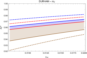
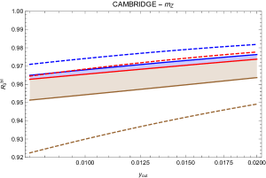
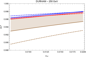
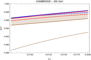
Figure 1: Theory predictions for $R_{3}^{b\ell}$ in the Durham (left plots) and Cambridge (right plots) jet-clustering algorithm at the $Z$-pole scale (upper plots) and $\sqrt{s}=250\leavevmode\nobreak\ {\mathrm{Ge\kern-0.90005ptV}}\,$ (lower plots). The dashed lines are LO, and the solid lines are NLO. The brown lines correspond to the theory predictions in terms of the pole mass and $\mu=\sqrt{s}$. The blue and red lines represent the theory predictions with the running mass and renormalization scales at $\mu=2\sqrt{s}$ and $\mu=\sqrt{s}/2$, respectively. The theory uncertainty is estimated from the spread of the results, and is given by the shadowed band at NLO.

Our reference input numerical values for the $b$-quark running and pole masses are taken from the world averages of the 2020 PDG [3]:

$$m_{b}(m_{b})=4.18^{+0.03}_{-0.02}\leavevmode\nobreak\ {\mathrm{Ge\kern-1.00006ptV}}\,\leavevmode\nobreak\ ,\qquad M_{b}=4.78(6)\leavevmode\nobreak\ {\mathrm{Ge\kern-1.00006ptV}}\,\leavevmode\nobreak\ ,$$ (9)

together with the corresponding values for the strong coupling, and the masses of the $Z$ and Higgs bosons

$$\alpha_{S}(m_{Z})=0.1179(10)\leavevmode\nobreak\ ,\qquad m_{Z}=91.1876(21)\leavevmode\nobreak\ {\mathrm{Ge\kern-1.00006ptV}}\,\leavevmode\nobreak\ ,\qquad m_{H}=125.10(14)\leavevmode\nobreak\ {\mathrm{Ge\kern-1.00006ptV}}\,\leavevmode\nobreak\ .$$ (10)

We use the analytic solutions to the two-loop renormalization group equations in QCD from Refs. [33, 34] to evolve the $b$-quark mass in Eq. (9) from low energies to higher energies,

$$m_{b}(m_{Z})=2.97(4)\leavevmode\nobreak\ {\mathrm{Ge\kern-1.00006ptV}}\,\leavevmode\nobreak\ ,$$ (11)

and then to the ILC 250 GeV scale in the SM

$$m_{b}(250\leavevmode\nobreak\ {\mathrm{Ge\kern-1.00006ptV}}\,)=2.75(4)\leavevmode\nobreak\ {\mathrm{Ge\kern-1.00006ptV}}\,\leavevmode\nobreak\ .$$ (12)

In Fig. 1 we show the theory predictions for $R_{3}^{b\ell}$. The experimental uncertainty in $R_{3}^{b\ell}$ necessary to extract the $b$-quark mass value with a given uncertainty can be estimated through the approximation

$$\Delta R_{3}^{b\ell}\sim\frac{2(1-R_{3}^{b\ell})}{m_{b}(\mu)}\,\Delta m_{b}(\mu)\leavevmode\nobreak\ .$$ (13)

This means, for example, that for a target uncertainty of $\Delta m_{b}(\mu)=0.2\leavevmode\nobreak\ {\mathrm{Ge\kern-1.00006ptV}}\,$, and given the results in Fig. 1, we need to reach a $0.5\%$ accuracy in $R_{3}^{b\ell}$ at the $Z$-pole and a challenging $0.5$ per mile at $\sqrt{s}=250\leavevmode\nobreak\ {\mathrm{Ge\kern-1.00006ptV}}\,$. This is consistent with Fig. 2 where we show the mass dependence of the theory predictions for $R_{3}^{b\ell}$.

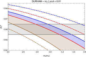
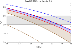
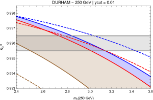
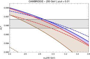
Figure 2: Mass dependence of $R_{3}^{b\ell}$. Same colour scheme as in Fig. 1. The horizontal band represents an Ansatz for the experimental measurement.

The theoretical uncertainty is estimated by considering the following sources:

• Renormalization scale: The renormalization scale $\mu$ in the theoretical expression (8) is varied from $\mu=\sqrt{s}/2$ to $\mu=2\sqrt{s}$ and half of the difference between the results obtained on $m_{b}(\mu)$ is taken as the renormalization scale uncertainty;

• Mass ambiguity: Starting from the NLO calculation of $R_{3}^{b\ell}$ in terms of the pole mass $M_{b}$, the value of $M_{b}$ could be extracted and transformed to $m_{b}(M_{b})$ which was later evolved to $m_{b}(m_{Z})$ by means of the RGE. This is also a valid procedure to extract $m_{b}(m_{Z})$. At infinite orders the result derived in this way and the one obtained directly from the original NLO calculation in terms of the running mass should be the same. The difference between the results obtained from the two procedures was then considered as a conservative indication of the size of the unknown higher order corrections;

• Strong coupling: the strong coupling $\alpha_{S}(m_{Z})$ from (10) is varied within its uncertainty. The spread of values obtained for $m_{b}(\mu)$ is added to the theory uncertainty. It provides a very small contribution in comparison to the renormalization scale uncertainty.

These uncertainty are evaluated quantitatively in Section 6.

3 Monte Carlo simulations

The projection for the bottom quark mass measurement is obtained from a detailed Monte Carlo simulation of the 250 GeV run at the ILC. All results reported in this note are obtained using Monte Carlo samples generated by the ILD concept group [35]. This work uses the same samples, signal definitions and reconstruction tools as a previous study described in [36].

The samples consist of events generated at leading order in QCD using the WHIZARD 1.95 [37, 38] event generator. The parton showering and hadronization are simulated by the Pythia 6.422 event generator [39]. QED initial state radiation (ISR) is simulated on top of the matrix element via CIRCE [40]. QCD final state radiation (FSR) is implemented by Pythia in the parton shower stage.

The LO generator setup lacks the formal precision to predict the value of $R_{3}^{b\ell}$ accurately. The Monte Carlo simulation is primarily used to assess the importance of hadronization and experimental effects. The central values of estimated observable is re-scaled, where needed, to the Next-to-leading order (NLO) QCD prediction described in Section 2. Studies on the implementation of NLO calculations in the WHIZARD 2 generator are ongoing, in collaboration with the Whizard authors, and may eventually be incorporated in the ILD simulation framework, but is left for a future publication.

All samples, signal and backgrounds, are generated assuming a longitudinal beam polarization of 100%. The configuration where the electron beam is left polarized and the positron beam is right-polarized is indicated as $e_{L}^{\mbox{\scriptsize-}}$$e_{R}^{\mbox{\scriptsize+}}$. The opposite configuration is labelled as $e_{R}^{\mbox{\scriptsize-}}$$e_{L}^{\mbox{\scriptsize+}}$. The statistics of the samples is limited and corresponds to integrated luminosity of 250 fb^-1for the signal events.

The ILC data taking program (ILC H20 program [31]) foresees a total integrated luminosity of 2000 fb^-1 shared between different beam polarizations schemes. Most of the luminosity will be collected in two samples of equal size of 900 fb^-1with the polarisation schemes $-+$ and $+-$. The $-+$ scheme stands for $Pol(e^{-})=P=-80\%$ and $Pol(e^{+})=P^{\prime}=+30\%$ and the $+-$ schems for $Pol(e^{-})=P=+80\%$ and $Pol(e^{+})=P^{\prime}=-30\%$. This is the so called H20 luminosity scenario for the ILC.

The signal, $e^{\mbox{\scriptsize-}}e^{\mbox{\scriptsize+}}\rightarrow Z^{*}/\gamma\rightarrow q\overline{q}$, cross section for different scenarios with fully polarised beams are listed in Table 2. The cross sections of the processes contributing to the background contamination are listed in Table 3, also for fully polarised beam scenarios. These backgrounds come from two different types of process. The first one is the so-called radiative return: when the energy of the ISR, $E_{\gamma}$ is large enough to produce a shift on the centre of mass energy of the hard interaction to produce a on-shell $Z$-boson in the process, $e^{\mbox{\scriptsize-}}e^{\mbox{\scriptsize+}}\gamma\rightarrow Z\gamma\rightarrow\gamma q\overline{q}$. Therefore, the $q$$\overline{q}$ in the final state are not produced at 250 GeV but at the $Z$-pole.

Polarization	$\sigma_{e^{\mbox{\scriptsize-}}e^{\mbox{\scriptsize+}}\rightarrow q\overline{q}}(E_{\gamma}<50\,{\mathrm{Ge\kern-1.00006ptV}}\,)$[fb]
	$b$$\overline{b}$	$c$$\overline{c}$	$q$$\overline{q}$ ($q=uds$)
$e_{L}^{\mbox{\scriptsize-}}$$e_{R}^{\mbox{\scriptsize+}}$	5970.9	8935.2	19347.6
$e_{R}^{\mbox{\scriptsize-}}$$e_{L}^{\mbox{\scriptsize+}}$	1352.1	3735.1	5920.4

Table 2: LO production cross section of quark pairs at 250 GeV of centre of mass using polarized beams.

Channel	$\sigma_{e_{L}^{\mbox{\scriptsize-}}e_{R}^{\mbox{\scriptsize+}}}$ [fb]	$\sigma_{e_{R}^{\mbox{\scriptsize-}}e_{L}^{\mbox{\scriptsize+}}}$ [fb]
$e^{\mbox{\scriptsize-}}e^{\mbox{\scriptsize+}}\rightarrow Z\gamma\rightarrow\gamma q\overline{q}(E_{\gamma}>50\,{\mathrm{Ge\kern-1.00006ptV}}\,)$	94895.3	60265.3
$e^{\mbox{\scriptsize-}}e^{\mbox{\scriptsize+}}\rightarrow WW\rightarrow q_{1}\bar{q_{2}}q_{3}\bar{q_{4}}$	14874.4	136.4
$e^{\mbox{\scriptsize-}}e^{\mbox{\scriptsize+}}\rightarrow ZZ\rightarrow q_{1}\bar{q_{1}}q_{2}\bar{q_{2}}$	1402.1	605.0
$e^{\mbox{\scriptsize-}}e^{\mbox{\scriptsize+}}\rightarrow HZ\rightarrow q_{1}\bar{q_{1}}q_{2}\bar{q_{2}}$	346.0	222.0

Table 3: Cross sections at 250 GeV for processes producing at least a pair of quarks (all flavours except $t$-quark).

The ILD detector geometry and the interaction of the particles with the detector are simulated within the Mokka framework interfaced with the GEANT4 toolkit [30, 41, 42].

4 Event selection

In this section, the main steps of the event selection are introduced.

Low-level object reconstruction

The simulated events are reconstructed using the standard ILCSoft toolkit, which includes algorithms for tracking [43] and vertex reconstruction, the Pandora particle flow algorithm [44], photon identification, jet clustering and flavour tagging algorithms. We refer to the description in Ref. [36] for details and only describe the jet clustering and flavour tagging steps in some detail.

The Particle Flow Objects reconstructed with the Pandora algorithm form the input to the jet clustering algorithm. For the initial jet clustering we use the generalised $k_{t}$ algorithm for $e^{\mbox{\scriptsize-}}$$e^{\mbox{\scriptsize+}}$ colliders as implemented in FastJet [45], with parameters $R=1.25$ and $p=1$, following the optimization in [36]. The algorithm is configured to reconstruct exactly two jets (exclusive clustering).

Flavour selection. The reconstruction of $R_{3}^{b\ell}$ requires the identification of the flavour of quarks in the $e^{+}e^{-}\rightarrow q\overline{q}(g)$ process. To this end the nominal ILD flavour tagging algorithm is applied on both jets. The LCFIPlus package [46] provides a vertex reconstruction algorithms. The jet flavour tag is assigned using boosted decision trees (BDTs) that take into account a number of variables from tracks and vertices. For each jet the LCFIPlus algorithm returns two tagging variables, $btag$ and $ctag$, which reflect the likelihood that the jet originated from the fragmentation of a $b$-quark or a $c$-quark, respectively. The likelihood distribution for the $e^{+}e^{-}\rightarrow q\overline{q}(g)$ at $\sqrt{s}=$ 250 GeV  is shown in Fig. 3, for the $e_{L}^{\mbox{\scriptsize-}}$$e_{R}^{\mbox{\scriptsize+}}$ configuration in the left panel and for the $e_{R}^{\mbox{\scriptsize-}}$$e_{L}^{\mbox{\scriptsize+}}$ configuration in the right panel. The contributions from the different processes, classified by the Monte Carlo truth information, are indicated with different fill colours in the histograms.

Events are assigned to the $b$-quark or $\ell$-quark sample based on a double tag, requiring that both jets satisfy the following criterion:

• For the $b$-quark sample: $btag>0.85$

• For the $\ell$-quark sample: $btag<0.4$ & $ctag<0.25$

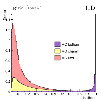
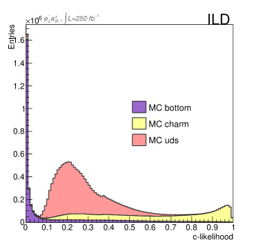
Figure 3: Distributions of b-likelihood(left) and c-likelihood(right) for left polarised $e^{+}e^{-}\to q\overline{q}$ sample.

The efficiency and purity of the flavour tag classification are summarized in Table 4 for $b$-quark and $\ell$-quarks. For comparison, the performance of the DELPHI selection is shown in the same table. The efficiency with which ILD expects to select the $b$-quark sample is approximately 80%, with a purity of nearly 98%. It thus exceeds the DELPHI results in both aspects very considerably, as might be expected from the advance in vertex detector technology since LEP era together with a more precise primary vertex reconstruction allowed by the higher energy of the jets and the excellent vertexing due to the smaller radius of the vacuum pipe. Also for the $\ell$-quark sample the $b$ and $c$-quark vetoes are expected to work somewhat more efficiently, and with much greater purity, than in the DELPHI analysis.

	$b$-quark		$\ell$-quarks
Experiment	Eff. [%]	Pur. [%]	Eff. [%]	Pur. [%]
DELPHI [19]	47%	86%	51%	82%
ILD (this note)	80%	98.7%	58%	96.1%

Table 4: Prospects for efficiency and purity of single jet tagging at ILD compared with the values published in [19] used as reference of the $R_{3}^{b\ell}$ experimental method.

Rejection of radiative return events. To clearly identify the scale of the process used to measure $m_{b}(m_{Z})$ events where a hard photon from Initial State Radiation (ISR) reduces the center-of-mass energy significantly are removed from the sample. The simplest way to remove these radiative-return events is to veto events with an energetic ISR photon. We therefore veto events with an energetic photon. However, for a large fraction of the cases, ISR photons are emitted at low angle and often the photon is lost in the beam pipe. Again following Ref. [36], we reject these events using angular and energy conservation criteria. For this analysis, cuts are applied on the invariant mass of the two-jet system and on the $K_{reco}$ quantity. This quantity is used as an estimator of the momentum of the ISR, $|\vec{k}|$ and it is defined as:

$$|\vec{k}|\approx K_{reco}=\frac{250\,\text{GeV}\cdot\sin{\Psi_{acol}}}{\sin{\Psi_{acol}}+\sin{\theta_{1}}+\sin{\theta_{2}}}$$ (14)

where the $\Psi_{acol}$ variable describes the acolinearity between the two reconstructed jets:

$$\sin{\Psi_{acol}}=\frac{|\vec{p}_{j_{1}}\times\vec{p}_{j_{2}}|}{|\vec{p}_{j_{1}}|\cdot|\vec{p}_{j_{1}}|}$$ (15)

and $\theta_{j}$ refers to the reconstructed polar angle of the jet-$j$ in the detector reference frame.

The cuts that aim to reduce the contamination by radiative-return events can be summarized as follows:

• no photons with $E_{\gamma}>$ 100 GeV

• no photon with $E_{\gamma}>$ 70 GeV  and $|\cos\theta|>$ 0.95

• $K_{reco}<50$ GeV

• $m_{2jets}>130$ GeV.

This selection removes approximately 99% of the radiative-return events, and a good fraction of the diboson background events, while keeping around 80% of our signal events.

Rejection of the boson pair production background. After the radiative-return and flavour selection, a significant background due to boson pair production still remains. In Ref. [36], this background [36] is rejected with a cut on the $y_{23}$ variable which is tightly connected to three-jet rates. To avoid a strong bias in the $R_{3}^{b\ell}$ measurement, we investigate other event shapes variables, motivated by the selection procedure described in [19]. In Fig. 4 we show the potential of the $Thrust$ variable to remove background events. This variable is defined as:

$$Thrust=\max\limits_{|\vec{n}|=1}(\frac{\sum\limits_{PFO}|\vec{n}\cdot\vec{p}_{PFO}|}{\sum\limits_{PFO}|\vec{p}_{PFO}|})$$ (16)

A mild cut is found to reduce the boson pair background strongly, with a minimal bias on the signal events. We therefore apply the following $WW/ZZ/ZH$ rejection cut:

• $Thrust$ > 0.8.

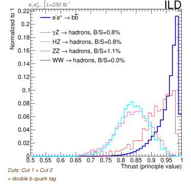
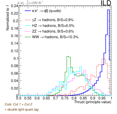
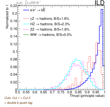
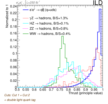
Figure 4: Distribution of the Thrust variable used to discriminate the remaining di-boson backgrounds from the signal events. The upper row presents the results for the $e_{L}^{\mbox{\scriptsize-}}$$e_{R}^{\mbox{\scriptsize+}}$ configuration, the lower row for $e_{R}^{\mbox{\scriptsize-}}$$e_{L}^{\mbox{\scriptsize+}}$. The plots in the leftmost panel are for $b$-quark production, the ones in the rightmost panel for $\ell$-quark (uds) production.

Selection efficiency and purity. The result of the selection procedure described above is summarized in Table 5. The efficiency for the $e^{+}e^{-}\rightarrow b\bar{b}(g)$ process is nearly 40% for both beam polarizations. The $\ell$-quark sample is selected with an efficiency slightly over 16%. The contamination by radiative-return events, that complicate the assignment of an unambiguous scale to the process, is controlled to the 1-2% level in both samples. The contribution to the event yield of other processes is expected to be order of 2-5% for the $\ell$-quark sample in the $e_{L}^{\mbox{\scriptsize-}}$$e_{R}^{\mbox{\scriptsize+}}$ configuration, and much smaller for the $b$-quark sample and the $e_{R}^{\mbox{\scriptsize-}}$$e_{L}^{\mbox{\scriptsize+}}$ beam polarization configuration.

$e_{L}^{\mbox{\scriptsize-}}$$e_{R}^{\mbox{\scriptsize+}}$
		B/S
	Signal Eff [%]	Rad. Return	$WW$	$ZZ$	$HZ$
T>0.8
$R_{3}^{\ell}$	16.5%	1.4%	5.1%	0.3%	0.0%
$R_{3}^{b}$	37.8%	1.2%	0.0%	0.6%	0.6%
T>0.85
$R_{3}^{\ell}$	16.2%	1.3%	2.3%	0.2%	0.0%
$R_{3}^{b}$	36.9%	1.2%	0.0%	0.3%	0.3%
$e_{R}^{\mbox{\scriptsize-}}$$e_{L}^{\mbox{\scriptsize+}}$
		B/S
	Signal Eff [%]	Rad. Return	$WW$	$ZZ$	$HZ$
T>0.8
$R_{3}^{\ell}$	16.7%	1.5%	0.1%	0.5%	0.0%
$R_{3}^{b}$	37.3%	1.9%	0.0%	1.4%	1.8%
T>0.85
$R_{3}^{\ell}$	16.4%	1.4%	0.0%	0.3%	0.0%
$R_{3}^{b}$	36.5%	1.8%	0.0%	0.9%	1.0%

Table 5: Cut flow for the signal and background events.

5 Measurement of $R_{3}^{b\ell}$ at $\sqrt{s}=$ 250 GeV 

Definition of the observable. The $R_{3}^{b\ell}$ observable is reconstructed by re-clustering the Particle Flow Objects in the selected events using the Cambridge algorithm [13]. This algorithm was used in the most precise DELPHI measurement, where it was shown to reduce the hadronization uncertainties compared to the Durham algorithm. In principle, one could explore the use of more robust algorithms [47], but as the NLO calculation of Section 2 is available for Cambridge, we stick to the Cambridge algorithm in the current study.

For a given flavour, $q$, after the full selection procedure we get a sample of events forced to be clustered as two jets and with both of them tagged as originated from a $q$-quark. The size of this sample is $N^{q}_{double-tag}$. Studying the internal structure of the jets using the Cambridge algorithm we determine how many of these events would be reconstructed as 3 jets, as a function of $y_{cut}$. The size of this sample is $N^{q,3-jets}_{double-tag}$. With these two distributions we define the three-jet rate as follows:

$$\left.R_{3}^{q}\right|_{reco}=\frac{N_{double-tag}^{q,3-jets}(y_{cut})}{N_{double-tag}^{q}}.$$ (17)

where $q$ indicates the quark flavour, and can take two values: $q=b$ or $q=\ell$. The double ratio $\left.R_{3}^{b\ell}\right|_{reco}$ is the ratio of $\left.R_{3}^{b}\right|_{reco}$ and $\left.R_{3}^{\ell}\right|_{reco}$, as in Eq. 4.

Monte Carlo results for $R_{3}^{b\ell}$. The value of $R_{3}^{b\ell}$ in signal events is shown as a function of $y_{cut}$ in Fig. 5.

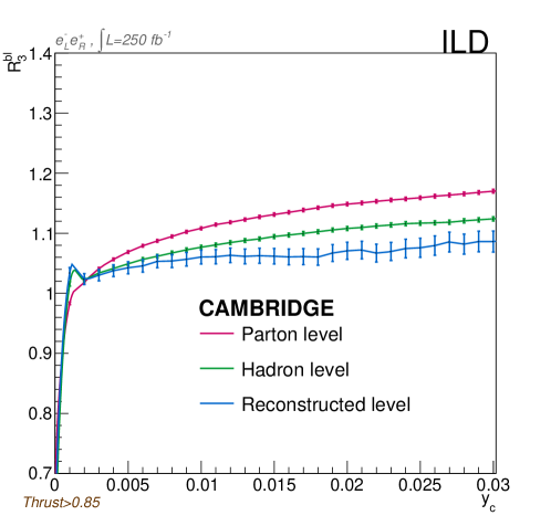
Figure 5: $R_{3}^{b\ell}$ distribution at parton level (red), at hadron level (green) and at the level of reconstructed objects (dark blue) applying the selection cuts described in the previous section. All curves correspond to signal events, without backgrounds. The central value for $R_{3}^{b\ell}$ predicted by the LO Monte Carlo is not reliable since the gluon radiation and the quark mass effects are only generated by the parton shower algorithm; only the difference between the curves are meaningful, indicating a size of the correction between generator levels.

The observable is defined at several different levels as shown in Fig. 5. The red markers, labelled as parton shower level, indicate the result that is obtained when the Cambridge clustering is applied to partons from the Pythia truth record after Final State Radiation. This level is closest  to the result of the fixed-order calculation reported in Section 2. The green markers, labelled as hadron level, indicate the result obtained when clustering stable final-state particles. The sets of points with blue markers indicate the result at the detector level, obtained when clustering particle flow objects.

Clearly, the observable is transformed in important ways by the parton shower and the hadronization into colour-neutral particles and by the response of the detector.

Correction to the parton level. To compare the measured value of $R_{3}^{b\ell}$ to a fixed-order calculation, the result must be corrected back to parton level. Following the same approach as Ref. [19], the result is unfolded with two correction factors:

$$\left.R_{3}^{b\ell}\right|_{parton}=C_{had}\times C_{det}\times\left.R_{3}^{b\ell}\right|_{reco}$$ (18)

The first correction factor, $C_{had}$, contains the correction to the parton level distribution, undoing the effect of hadronization modelling.

The second factor, $C_{det}$, corrects the effect of the detector resolution and any bias introduced by the detector acceptance and efficiency. It can be broken down in terms of the signal selection efficiency $\epsilon_{sel}$, the background selection efficiency $\epsilon_{bkg}$ and the flavour tagging efficiency $\epsilon_{q}$ and mis-tag probability $\epsilon_{q}^{\prime}$:

$$\left.R_{3}^{q}(y_{cut})\right|_{reco}=\frac{\epsilon_{sel}\cdot\left[\epsilon_{q}^{2}\sigma_{q\overline{q}}^{3jet}(y_{cut})+\epsilon_{q^{\prime}}^{2}\sigma_{q^{\prime}\bar{q}}^{3jet}(y_{cut})\right]+\epsilon_{bkg}\sigma_{bkg}^{3jet}(y_{cut})}{\epsilon_{sel}\cdot\left[\epsilon_{q}^{2}\sigma_{q\overline{q}}+\epsilon_{q^{\prime}}^{2}\sigma_{q^{\prime}\bar{q}}\right]+\epsilon_{bkg}\sigma_{bkg}}.$$ (19)

The values obtained from the Monte Carlo simulation for these correction factors are shown in the Fig. 6, separately for the two polarization configurations and for the signal and background samples.

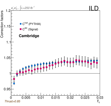
Figure 6: $C^{had}$ and $C^{det}$ for only signal and the two $100\%$ beam polarisation cases used in our simulated samples.

For a choice of $y_{cut}=$ 0.01, the correction for hadronization and detector effects are of the order of 2-3%. The correction for the background samples is found to be very similar to that of the signal. The systematic uncertainty on the correction is expected to be a fraction of the correction. We estimate these systematic uncertainties in the following.

Statistical uncertainty. The statistical uncertainty of the $R_{3}^{b\ell}$ measurement with an integrated luminosity of 2 ab^-1 at $\sqrt{s}=$ 250 GeV  is, combining both channels, of 1 GeV , as explained in Section 6.

Estimation of systematic uncertainties. The main sources of uncertainty in the DELPHI analysis of Ref. [19] correspond to the hadronization modelling and the contamination of other quarks in the double tagged samples. We proceed to estimate the dominant systematic uncertainties for the measurement at 250 GeV .

Flavour tagging. As shown in the Table 4, the tagging capabilities of ILD are expected to be far superior than those of the LEP experiments, therefore reducing the miss-tag rates considerably. The flavour tagging efficiencies can be determined in situ using the double and single tag rates. Ref. [36] predicts a precision at the 0.1-0.5% level. Propagating these uncertainties to the $R_{3}^{b\ell}$ measurement from Eq. 19 one obtains an uncertainty of 0.07% for the $e_{L}^{\mbox{\scriptsize-}}$$e_{R}^{\mbox{\scriptsize+}}$ configuration and 0.06% for the $e_{R}^{\mbox{\scriptsize-}}$$e_{L}^{\mbox{\scriptsize+}}$ beam polarization. The other stages of the event selection may also bias the result, but its effect is expected to cancel to a good extent in the double tag rate.

Hadronization. The uncertainties related to the hadronization correction are expected to be smaller than at LEP, thanks to progress in Monte Carlo generators and the important data set collected at the Tevatron and LHC since LEP era. On general grounds, one expects that the impact of hadronization is further reduced at higher centre-of-mass energies. We assume that the this uncertainty is a half of that in the DELPHI measurement of Ref. [19], which leads to an 0.1% uncertainty on $R_{3}^{b\ell}$.

Background modelling. In contrast with the analysis running at the $Z$-pole, the analysis at $\sqrt{s}=$ 250 GeV  is sensitive to the modelling of the backgrounds. Assuming that the experiment can control the normalization of the remaining di-boson background at the per cent level, the uncertainty on $R_{3}^{b\ell}$ is approximately 0.22% for the $e_{L}^{\mbox{\scriptsize-}}$$e_{R}^{\mbox{\scriptsize+}}$ configuration and 0.1% for the $e_{R}^{\mbox{\scriptsize-}}$$e_{L}^{\mbox{\scriptsize+}}$ measurement.

The estimates for the dominant uncertainties are summarized in Table 6.

$C_{had}$ Systematic Unc.
Source	Estimation	comments
hadronization modelling	0.1 %	Assumed to be half the uncertainty evaluated for LEP
$C_{det}$ Systematic Unc. ($e_{L}^{\mbox{\scriptsize-}}$$e_{R}^{\mbox{\scriptsize+}}$)
flavour tagging	0.07 %	assuming flavour tagging uncertainties as estimated in [36]
pre-selection efficiency	0.06 %	as estimated in [36]
$Z\gamma/WW/HZ/ZZ$ modelling	0.20 %	assuming modelling uncertainties at the per cent level. It assumes a moderated cut in the thrust of the event which may required further studies to reject possible biases on the observable due to this cut.
total	0.22 %	dominated by the $WW$ contamination to $R_{3}^{\ell}$
$C_{det}$ Systematic Unc. ($e_{R}^{\mbox{\scriptsize-}}$$e_{L}^{\mbox{\scriptsize+}}$)
flavour tagging	0.06 %	assuming flavour tagging uncertainties as estimated in [36]
pre-selection efficiency	0.06 %	as estimated in [36]
$Z\gamma/WW/HZ/ZZ$ modelling	0.1 %	Assuming modelling uncertainties at the per cent level. No specific cuts are needed for the removal of the backgrounds.
total	0.13 %	dominated by the $ZZ$ and radiative return contamination to $R_{3}^{b}$

Table 6: Comprehensive assessment of the expected main systematic uncertainties on the measurement of $R_{3}^{b\ell}$.

6 Prospects for bottom-quark mass measurements at the ILC

In this section we present the estimates of the uncertainty on the bottom mass that can be achieved in the envisaged runs at the ILC. Apart from the main result of this note, the prospect for the measurement of $m_{b}(250{\mathrm{Ge\kern-1.00006ptV}}\,)$, we extrapolate the precision achieved at LEP to the GigaZ run.

Measurement of $m_{b}(250\leavevmode\nobreak\ {\mathrm{Ge\kern-1.00006ptV}}\,)$ in the "Higgs factory" run. We estimate the precision of the bottom quark mass measurement at $\sqrt{s}=$ 250 GeV from the projection for $R_{3}^{b\ell}$ in Section 5. The statistical and systematic uncertainties are estimated using the mass sensitivity of the $R_{3}^{b\ell}$ observable as approximated in Eq. 13. A total integrated luminosity of 2 ab^-1 is envisaged in the standard ILC operating scenario, with 40% of the data collected in the LR polarization, and 40% in the RL configuration. The central value for $R_{3}^{b\ell}$ is taken to be the SM prediction, $R_{3}^{b\ell}=$ 0.996, obtained with the NLO QCD calculation. The statistical uncertainty is estimated for a value of $R_{3}^{b}\sim R_{3}^{\ell}\sim 0.3$ for $y^{CAMB}_{cut}=0.01$. The systematic uncertainties on the $R_{3}^{b\ell}$ measurement are propagated to the mass determination using the information from the Eq. 13 and the Fig. 1 (bottom right). The theoretical uncertainty is estimated from variations in the renormalization scale and mass scheme and the value of the strong coupling constant in Section 2. The result is divided by two to anticipate a future NNLO calculation of the observable.

This procedure yields the following expected precision for the mass measurements performed with the two main beam polarization configurations:

$$\Delta m_{b}(-+)=\pm 0.85(stat.)\pm 0.34(had.)\pm 0.75(exp.)\pm 0.07(th.)\leavevmode\nobreak\ {\mathrm{Ge\kern-1.00006ptV}}\,$$ (20)

$$\Delta m_{b}(+-)=\pm 1.53(stat.)\pm 0.34(had.)\pm 0.44(exp.)\pm 0.07(th.)\leavevmode\nobreak\ {\mathrm{Ge\kern-1.00006ptV}}\,\$$ (21)

The two results are combined with the best linear unbiased estimator procedure (BLUE [48]), that takes into account the correlations among systematic uncertainties (100% for hadronization and theory uncertainties, 50% for the experimental systematics). The projected uncertainty for the mass measurement is given by:

$$\Delta m_{b}(250\leavevmode\nobreak\ {\mathrm{Ge\kern-1.00006ptV}}\,)=1.0\leavevmode\nobreak\ {\mathrm{Ge\kern-1.00006ptV}}\,=\pm 0.76(stat)\pm 0.59(syst.)\pm 0.34(had.)\pm 0.07(th.)\leavevmode\nobreak\ {\mathrm{Ge\kern-1.00006ptV}}\,$$ (22)

The precision on the high-scale is not directly competitive with measurements at lower scales, but extends the analysis to scales not probed by previous experiments.

Measurement of $m_{b}(m_{Z})$ in the "GigaZ" scenario. The "GigaZ" run is an option in the ILC program, where an integrated luminosity of $\sim$ 100 fb^-1is collected at the $Z$-pole [31]. This run is thus expected to generate two orders of magnitude more $b$$\overline{b}$ pairs than LEP1. With the larger data set and the excellent flavour tagging performance the ILC experiments can improve the measurement of $m_{b}(m_{Z})$ very considerably.

The statistical uncertainty is expected to become sub-dominant. We assume that the theory uncertainties are reduced by a factor two with respect to the LEP result, anticipating an NNLO calculation of the three-jet rate. Also the hadronization uncertainty is divided by two, which requires an important improvement of the hadronization model. The experimental uncertainty is estimated by assuming the same flavour tagging capabilities than at 250 GeV. Compared to the 250 GeV  estimate, the impact of systematic uncertainties is much reduced. This is a result of the much larger mass sensitivity at the $Z$-pole, as antipicated in Section 2.

The expected precision of the $b$-quark mass measurement is then:

$$\Delta m_{b}(m_{Z})=0.12\leavevmode\nobreak\ {\mathrm{Ge\kern-1.00006ptV}}\,=\pm 0.02(stat.)\pm 0.09(had.)\pm 0.02(exp.)\pm 0.06(th.)\leavevmode\nobreak\ {\mathrm{Ge\kern-1.00006ptV}}\,$$ (23)

The total uncertainty of 0.12 GeV , improves considerably on the combination of the LEP/SLD measurements.

7 Conclusions and summary

The mass measurements at the ILC can provide an important contribution to the characterization of the scale evolution of the $b$-quark mass. To visualize their impact, the projections obtained in this section are added to Fig. 7. It furthermore includes the world average for the mass measurements at low scale, given by the PDG value for $m_{b}(m_{b})$ [3] and the LEP and SLD measurements [14, 15, 16, 17, 18, 19, 6, 20] of $m_{b}(m_{Z})$. The reference value of $m_{b}(m_{b})=$ 4.18 GeV is evolved to higher scale using the RGE implemented in the REvolver code [49].

The ILC measurements are expected to bring considerable additional evidence for the evolution of the bottom quark mass. The measurement of $R_{3}^{b\ell}$ at $\sqrt{s}=$ 250 GeV has a modest precision, limited by the much reduced mass sensitivity, but extends the test of the QCD evolution to energies not probed by previous experiments. The GigaZ program offers the potential of a considerable improvement of the measurement of $m_{b}(m_{Z})$.

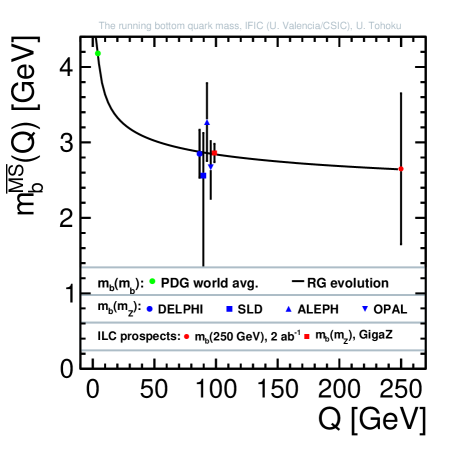
Figure 7: The evolution of the bottom-quark $\overline{MS}$ mass with the scale $Q$. The black line corresponds to the QCD prediction, obtained from the RGE implemented in the REvolver code [49] for four loops and input values for $\alpha_{s}(m_{Z})$ and $m_{b}(m_{b})$ given by the PDG world average [3] (see Eqs. 9 and 10). The reference bottom quark mass is shown in a green marker. The blue markers indicate the results of four measurements at LEP and by SLD in Table 1. The red markers correspond to the projections obtained in this note.

References

- [1] Y. Kiyo, G. Mishima and Y. Sumino, Determination of mc and mb from quarkonium 1S energy levels in perturbative QCD, Phys. Lett. B752 (2016) 122–127, [1510.07072].
- [2] A. Penin and N. Zerf, Bottom Quark Mass from Sum Rules to , JHEP 04 (2014) 120, [1401.7035].
- [3] Particle Data Group collaboration, P. Zyla et al., Review of Particle Physics, PTEP 2020 (2020) 083C01.
- [4] M. S. Bilenky, G. Rodrigo and A. Santamaria, Three jet production at LEP and the bottom quark mass, Nucl. Phys. B 439 (1995) 505–535, [hep-ph/9410258].
- [5] G. Rodrigo, A. Santamaria and M. S. Bilenky, Do the quark masses run? Extracting from LEP data, Phys. Rev. Lett. 79 (1997) 193–196, [hep-ph/9703358].
- [6] M. S. Bilenky, S. Caberera, J. Fuster, S. Marti, G. Rodrigo and A. Santamaria, m(b)(m(Z)) from jet production at the Z peak in the Cambridge algorithm, Phys. Rev. D60 (1999) 114006, [hep-ph/9807489].
- [7] G. Rodrigo, M. S. Bilenky and A. Santamaria, Quark mass effects for jet production in e+ e- collisions at the next-to-leading order: Results and applications, Nucl. Phys. B 554 (1999) 257–297, [hep-ph/9905276].
- [8] W. Bernreuther, A. Brandenburg and P. Uwer, Next-to-leading order QCD corrections to three jet cross-sections with massive quarks, Phys. Rev. Lett. 79 (1997) 189–192, [hep-ph/9703305].
- [9] A. Brandenburg and P. Uwer, Next-to-leading order QCD corrections and massive quarks in e+ e- — three jets, Nucl. Phys. B 515 (1998) 279–320, [hep-ph/9708350].
- [10] P. Nason and C. Oleari, Next-to-leading order corrections to momentum correlations in Z0 — b anti-b, Phys. Lett. B 407 (1997) 57–60, [hep-ph/9705295].
- [11] P. Nason and C. Oleari, Next-to-leading order corrections to the production of heavy flavor jets in e+ e- collisions, Nucl. Phys. B 521 (1998) 237–273, [hep-ph/9709360].
- [12] S. Catani, Y. L. Dokshitzer, M. Olsson, G. Turnock and B. Webber, New clustering algorithm for multi - jet cross-sections in e+ e- annihilation, Phys. Lett. B 269 (1991) 432–438.
- [13] Y. L. Dokshitzer, G. Leder, S. Moretti and B. Webber, Better jet clustering algorithms, JHEP 08 (1997) 001, [hep-ph/9707323].
- [14] DELPHI collaboration, P. Abreu et al., at , Phys. Lett. B418 (1998) 430–442.
- [15] SLD collaboration, K. Abe et al., An Improved test of the flavor independence of strong interactions, Phys. Rev. D59 (1999) 012002, [hep-ex/9805023].
- [16] A. Brandenburg, P. N. Burrows, D. Muller, N. Oishi and P. Uwer, Measurement of the running b quark mass using e+ e- —> b anti-b g events, Phys. Lett. B468 (1999) 168–177, [hep-ph/9905495].
- [17] ALEPH collaboration, R. Barate et al., A Measurement of the b quark mass from hadronic Z decays, Eur. Phys. J. C18 (2000) 1–13, [hep-ex/0008013].
- [18] OPAL collaboration, G. Abbiendi et al., Determination of the b quark mass at the Z mass scale, Eur. Phys. J. C21 (2001) 411–422, [hep-ex/0105046].
- [19] DELPHI collaboration, J. Abdallah et al., Determination of the b quark mass at the M(Z) scale with the DELPHI detector at LEP, Eur. Phys. J. C46 (2006) 569–583, [hep-ex/0603046].
- [20] DELPHI collaboration, J. Abdallah et al., Study of b-quark mass effects in multijet topologies with the DELPHI detector at LEP, Eur. Phys. J. C55 (2008) 525–538, [0804.3883].
- [21] A. Gizhko et al., Running of the Charm-Quark Mass from HERA Deep-Inelastic Scattering Data, Phys. Lett. B775 (2017) 233–238, [1705.08863].
- [22] CMS collaboration, Running of the top quark mass from proton-proton collisions at 13 TeV, 1909.09193.
- [23] S. Catani, S. Devoto, M. Grazzini, S. Kallweit and J. Mazzitelli, Top-quark pair hadroproduction at NNLO: differential predictions with the mass, JHEP 08 (2020) 027, [2005.00557].
- [24] M. Boronat, E. Fullana, J. Fuster, P. Gomis, A. Hoang, V. Mateu et al., Top quark mass measurement in radiative events at electron-positron colliders, Phys. Lett. B 804 (2020) 135353, [1912.01275].
- [25] K. Bora, Updated values of running quark and lepton masses at GUT scale in SM, 2HDM and MSSM, Horizon 2 (2013) 112, [1206.5909].
- [26] S. Chigusa and T. Moroi, Bottom-tau unification in a supersymmetric model with anomaly-mediation, Phys. Rev. D 94 (Aug, 2016) 035016.
- [27] ILD Concept Group collaboration, H. Abramowicz et al., International Large Detector: Interim Design Report, 2003.01116.
- [28] P. Bambade et al., The International Linear Collider: A Global Project, 1903.01629.
- [29] T. Behnke et al., The International Linear Collider Technical Design Report - Volume 1-4, 1306.6327.
- [30] GEANT4 collaboration, S. Agostinelli et al., GEANT4: A Simulation toolkit, Nucl.Instrum.Meth. A506 (2003) 250–303.
- [31] T. Barklow, J. Brau, K. Fujii, J. Gao, J. List, N. Walker et al., ILC Operating Scenarios, 1506.07830.
- [32] K. Hagiwara, T. Kuruma and Y. Yamada, Three jet distributions from the one loop Z g g vertex at e+ e- colliders, Nucl. Phys. B 358 (1991) 80–96.
- [33] G. Rodrigo, A. Pich and A. Santamaria, Alpha-s (m(Z)) from tau decays with matching conditions at three loops, Phys. Lett. B 424 (1998) 367–374, [hep-ph/9707474].
- [34] G. Rodrigo and A. Santamaria, QCD matching conditions at thresholds, Phys. Lett. B 313 (1993) 441–446, [hep-ph/9305305].
- [35] H. Abramowicz et al., The International Linear Collider Technical Design Report - Volume 4: Detectors, 1306.6329.
- [36] A. Irles, R. Poeschl and F. Richard, Methods for b quark EW couplings measurements at ILC250 with 2000 fb-1: a tecnical review, xxxxxxxx.
- [37] W. Kilian, T. Ohl and J. Reuter, WHIZARD: Simulating Multi-Particle Processes at LHC and ILC, Eur. Phys. J. C71 (2011) 1742, [0708.4233].
- [38] M. Moretti, T. Ohl and J. Reuter, O’Mega: An Optimizing matrix element generator, hep-ph/0102195.
- [39] T. Sjöstrand, S. Mrenna and P. Skands, PYTHIA 6.4 physics and manual, Journal of High Energy Physics 2006 (may, 2006) 026–026.
- [40] T. Ohl, CIRCE version 1.0: Beam spectra for simulating linear collider physics, Comput. Phys. Commun. 101 (1997) 269–288, [hep-ph/9607454].
- [41] J. Allison et al., Geant4 developments and applications, IEEE Trans. Nucl. Sci. 53 (2006) 270.
- [42] J. Allison et al., Recent developments in Geant4, Nucl. Instrum. Meth. A835 (2016) 186–225.
- [43] F. Gaede, S. Aplin, R. Glattauer, C. Rosemann and G. Voutsinas, Track reconstruction at the ILC: the ILD tracking software, J. Phys. Conf. Ser. 513 (2014) 022011.
- [44] J. S. Marshall and M. A. Thomson, The Pandora software development kit for particle flow calorimetry, J. Phys. Conf. Ser. 396 (2012) 022034.
- [45] M. Cacciari, G. P. Salam and G. Soyez, FastJet user manual, Eur. Phys. J. C72 (2012) 1896, [1111.6097].
- [46] T. Suehara and T. Tanabe, LCFIPlus: A Framework for Jet Analysis in Linear Collider Studies, Nucl. Instrum. Meth. A808 (2016) 109–116, [1506.08371].
- [47] M. Boronat, J. Fuster, I. Garcia, P. Roloff, R. Simoniello and M. Vos, Jet reconstruction at high-energy electron–positron colliders, Eur. Phys. J. C78 (2018) 144, [1607.05039].
- [48] R. Nisius, BLUE: combining correlated estimates of physics observables within ROOT using the Best Linear Unbiased Estimate method, 2001.10310.
- [49] A. H. Hoang, C. Lepenik and V. Mateu, REvolver: Automated running and matching of couplings and masses in QCD, 2102.01085.