GPS-denied Navigation: Attitude, Position, Linear Velocity, and Gravity Estimation with Nonlinear Stochastic Observer

Abstract

Successful navigation of a rigid-body traveling with six degrees of freedom (6 DoF) requires accurate estimation of attitude, position, and linear velocity. The true navigation dynamics are highly nonlinear and are modeled on the matrix Lie group of $\mathbb{SE}_{2}(3)$. This paper presents novel geometric nonlinear continuous stochastic navigation observers on $\mathbb{SE}_{2}(3)$ capturing the true nonlinearity of the problem. The proposed observers combines IMU and landmark measurements. It efficiently handles the IMU measurement noise. The proposed observers are guaranteed to be almost semi-globally uniformly ultimately bounded in the mean square. Quaternion representation is provided. A real-world quadrotor measurement dataset is used to validate the effectiveness of the proposed observers in its discrete form.

I Introduction

Autonomous navigation would be infeasible without robust algorithms that enable accurate pose (i.e. attitude and position) and velocity estimation of a rigid-body. The challenge of attitude estimation, an essential component of pose, has been explored extensively over the past three decades [1, 2, 3, 4, 5]. Attitude can be defined given at least two observations in the inertial-frame and their measurements in the body-frame. For instance, a typical low-cost inertial measurement unit (IMU) module includes a magnetometer and an accelerometer which supply the two necessary body-frame measurements and a gyroscope which provides measurements of angular velocity. The main shortcoming of low-cost sensors is the high level of noise. Multiple solutions tackle attitude measurement uncertainty in attitude estimation, namely Gaussian filters [2], nonlinear deterministic filters on the Special Orthogonal Group $\mathbb{SO}(3)$ [3, 5], and nonlinear stochastic filters on $\mathbb{SO}(3)$ [4, 1]. In contrast, pose estimation requires a vision unit in addition to an IMU. Initially, Gaussian filters dominated the area of pose estimation. In the last few years, nonlinear deterministic filters on the Special Euclidean Group $\mathbb{SE}(3)$ [6, 7] and nonlinear stochastic filters on $\mathbb{SE}(3)$ [8, 9, 10] have been shown to be more effective. Pose estimation algorithms rely on measurements of angular and linear velocity [8]. In practice, linear velocity information is not attainable in case of 1) a GPS-denied environment and 2) a vehicle equipped with low-cost sensors.

The true six degrees of freedom (6 DoF) navigation dynamics are a combination of attitude, position, and linear velocity dynamics. The dynamics are highly nonlinear, are modeled on the Lie group of $\mathbb{SE}_{2}(3)$, are neither right nor left invariant, and rely on angular velocity and acceleration. The navigation problem has been approached using Gaussian filters, for instance, [11]. Other solutions that attempted mimicking the true navigation dynamics include a Riccati observer [12] and an invariant extended Kalman filter (IEKF) on $\mathbb{SE}_{2}(3)$ [13].

Considering the true nature of the navigation dynamics, this paper proposes novel nonlinear stochastic navigation observers on $\mathbb{SE}_{2}(3)$ that 1) mimics the true navigation dynamics; 2) estimates rigid-body’s attitude, position, linear velocity, and unknown gravity; and 3) relies on measurements of angular velocity and acceleration. The noise associated with IMU measurements is successfully handled. The closed loop signals are guaranteed to be almost semi-globally uniformly ultimately bounded (SGUUB) in the mean square. The novel solutions is shown to be cost-effective at a low sampling rate using a real-world dataset.

The rest of the paper is organized as follows: Section II introduces important math notation and the preliminaries, and formulates the navigation problem in a stochastic sense. Section III presents a novel nonlinear stochastic navigation observer. Section IV presents the obtained results. Finally, Section V summarizes the work.

II Problem Formulation

II-A Preliminaries

In this paper, sets of real numbers, nonnegative real numbers, and a real $n$-by-$m$ dimensional space are defined by $\mathbb{R}$, $\mathbb{R}_{+}$, and $\mathbb{R}^{n\times m}$, respectively. For $x\in\mathbb{R}^{n}$ and $M\in\mathbb{R}^{n\times m}$, $||x||=\sqrt{x^{\top}x}$ is the Euclidean norm of $x$ and $||M||_{F}=\sqrt{{\rm Tr}\{MM^{*}\}}$ is the Frobenius norm of $M$ with $*$ being a conjugate transpose. $\mathbf{I}_{n}$ denotes an $n$-by-$n$ identity matrix, while $0_{n\times m}$ and $1_{n\times m}$ denote $n$-by-$m$ dimensional matrices of zeros and ones, respectively. A set of eigenvalues of $M\in\mathbb{R}^{n\times n}$ is described by $\lambda(M)=\{\lambda_{1},\lambda_{2},\ldots,\lambda_{n}\}$ with $\overline{\lambda}_{M}=\overline{\lambda}(M)$ being the maximum value and $\underline{\lambda}_{M}=\underline{\lambda}(M)$ being the minimum value of $\lambda(M)$. $\mathbb{P}\{\cdot\}$ represents probability and $\mathbb{E}[\cdot]$ denotes an expected value. $\left\{\mathcal{I}\right\}$ represents fixed inertial-frame and $\left\{\mathcal{B}\right\}$ denotes fixed body-frame. Rigid-body’s attitude is defined by $R\in\mathbb{SO}\left(3\right)$ where $\mathbb{SO}(3)=\{R\in\mathbb{R}^{3\times 3}|RR^{\top}=R^{\top}R=\mathbf{I}_{3}\text{, }{\rm det}(R)=+1\}$ with ${\rm det}(\cdot)$ being a determinant. $\mathfrak{so}(3)$ defines the Lie algebra of $\mathbb{SO}(3)$ with $\mathfrak{so}\left(3\right)=\{[x]_{\times}\in\mathbb{R}^{3\times 3}|[x]_{\times}^{\top}=-[x]_{\times},x\in\mathbb{R}^{3}\}$. Note that $[x]_{\times}$ is a skew symmetric matrix such that

$$\left[x\right]_{\times} =\left[\begin{array}[]{ccc}0&-x_{3}&x_{2}\\ x_{3}&0&-x_{1}\\ -x_{2}&x_{1}&0\end{array}\right]\in\mathfrak{so}\left(3\right),\hskip 9.00002ptx=\left[\begin{array}[]{c}x_{1}\\ x_{2}\\ x_{3}\end{array}\right]$$

The inverse mapping of $[\cdot]_{\times}$ follows the map $\mathbf{vex}:\mathfrak{so}\left(3\right)\rightarrow\mathbb{R}^{3}$ with $\mathbf{vex}([x]_{\times})=x,\forall x\in\mathbb{R}^{3}$. The anti-symmetric projection on $\mathfrak{so}\left(3\right)$ is represented by $\boldsymbol{\mathcal{P}}_{a}(A)=\frac{1}{2}(A-A^{\top})\in\mathfrak{so}\left(3\right),\forall A\in\mathbb{R}^{3\times 3}$. $\boldsymbol{\Upsilon}=\mathbf{vex}\circ\boldsymbol{\mathcal{P}}_{a}$ describes a composition mapping where $\boldsymbol{\Upsilon}(A)=\mathbf{vex}(\boldsymbol{\mathcal{P}}_{a}(A))\in\mathbb{R}^{3},\forall A\in\mathbb{R}^{3\times 3}$. The Euclidean distance of $R\in\mathbb{SO}\left(3\right)$ is described by

$$||R||_{{\rm I}}={\rm Tr}\{\mathbf{I}_{3}-R\}/4\in\left[0,1\right]$$ (1)

where $-1\leq{\rm Tr}\{R\}\leq 3$ and $||R||_{{\rm I}}=\frac{1}{8}||\mathbf{I}_{3}-R||_{F}^{2}$, see [4, 1]. Consider a rigid-body navigating in 3D space where its attitude, position, and velocity are termed $R\in\mathbb{SO}\left(3\right)$, $P\in\mathbb{R}^{3}$, and $V\in\mathbb{R}^{3}$, respectively, with $R\in\{\mathcal{B}\}$ and $P,V\in\{\mathcal{I}\}$. Let $\mathbb{SE}_{2}\left(3\right)=\mathbb{SO}\left(3\right)\times\mathbb{R}^{3}\times\mathbb{R}^{3}\subset\mathbb{R}^{5\times 5}$ be the extended form of $\mathbb{SE}\left(3\right)=\mathbb{SO}\left(3\right)\times\mathbb{R}^{3}\subset\mathbb{R}^{4\times 4}$ with

$$\mathbb{SE}_{2}\left(3\right) =\{\left.X\in\mathbb{R}^{5\times 5}\right|R\in\mathbb{SO}\left(3\right),P,V\in\mathbb{R}^{3}\}$$ (2)

$$X=\Psi( R,P,V)=\left[\begin{array}[]{ccc}R&P&V\\ 0_{1\times 3}&1&0\\ 0_{1\times 3}&0&1\end{array}\right]\in\mathbb{SE}_{2}\left(3\right)$$ (6)

$X\in\mathbb{SE}_{2}\left(3\right)$ denotes a homogeneous navigation matrix which is assumed to be bounded. The tangent space of $\mathbb{SE}_{2}\left(3\right)$ at point $X$ is $T_{X}\mathbb{SE}_{2}\left(3\right)\in\mathbb{R}^{5\times 5}$. Define a submanifold $\mathcal{U}_{\mathcal{M}}=\mathfrak{so}\left(3\right)\times\mathbb{R}^{3}\times\mathbb{R}^{3}\times\mathbb{R}\subset\mathbb{R}^{5\times 5}$ such that

$$\mathcal{U}_{\mathcal{M}} =\left\{\left.u([\Omega\text{$]_{\times}$},V,a,\kappa)\right|[\Omega\text{$]_{\times}$}\in\mathfrak{so}(3),V,a\in\mathbb{R}^{3},\kappa\in\mathbb{R}\right\}$$

$$u( [\Omega\text{$]_{\times}$},V,a,\kappa)=\left[\begin{array}[]{ccc}[\Omega\text{$]_{\times}$}&V&a\\ 0_{1\times 3}&0&0\\ 0_{1\times 3}&\kappa&0\end{array}\right]\in\mathcal{U}_{\mathcal{M}}\subset\mathbb{R}^{5\times 5}$$ (10)

with $\Omega\in\mathbb{R}^{3}$, $V\in\mathbb{R}^{3}$, and $a\in\mathbb{R}^{3}$ being the rigid-body’s true angular velocity, linear velocity, and apparent acceleration composed of all non-gravitational forces affecting the rigid-body, respectively, where $\Omega,a\in\{\mathcal{B}\}$.

II-B Measurements and Dynamics

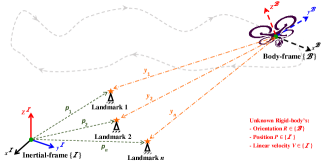
Figure 1: Navigation estimation problem.

The true dynamics of the homogeneous navigation matrix in (6) are as follow:

$$\begin{cases}\dot{R}&=R\left[\Omega\right]_{\times}\\ \dot{P}&=V\\ \dot{V}&=Ra+\overrightarrow{\mathtt{g}}\end{cases}\hskip 10.00002pt\equiv\hskip 10.00002pt\underbrace{\dot{X}=XU-\mathcal{\mathcal{G}}X}_{\text{Compact form}}$$ (11)

with $\overrightarrow{\mathtt{g}}$ denoting a gravity vector. The left portion of (11) represents the detailed navigation dynamics, while the right portion is its equivalent compact form with $X=\left[\begin{array}[]{ccc}R&P&V\\ 0_{1\times 3}&1&0\\ 0_{1\times 3}&0&1\end{array}\right]\in\mathbb{SE}_{2}\left(3\right)$, $U=u([\Omega\text{$]_{\times}$},0_{3\times 1},a,1)=\left[\begin{array}[]{ccc}[\Omega\text{$]_{\times}$}&0_{3\times 1}&a\\ 0_{1\times 3}&0&0\\ 0_{1\times 3}&1&0\end{array}\right]\in\mathcal{U}_{\mathcal{M}}$, and $\mathcal{\mathcal{G}}=u(0_{3\times 3},0_{3\times 1},-\overrightarrow{\mathtt{g}},1)=\left[\begin{array}[]{ccc}0_{3\times 3}&0_{3\times 1}&-\overrightarrow{\mathtt{g}}\\ 0_{1\times 3}&0&0\\ 0_{1\times 3}&1&0\end{array}\right]\in\mathcal{U}_{\mathcal{M}}$, visit (10). Note that $\dot{X}:\mathbb{SE}_{2}\left(3\right)\times\mathcal{U}_{\mathcal{M}}\rightarrow T_{X}\mathbb{SE}_{2}\left(3\right)$. The components of the navigation matrix $X$, namely $R$, $P$, and $V$, become completely unknown when the vehicle is equipped with low-cost sensors in a GPS-denied environment. Fig. 1 depicts the navigation problem. Availability of a set of sensor measurements enables the estimation of $X$. Consider a group of $n$ landmarks observed in $\left\{\mathcal{I}\right\}$ and measured in $\left\{\mathcal{B}\right\}$ [8, 9, 10]:

$$\overline{y}_{i} =X^{-1}\overline{p}_{i}+[(n_{i}^{y})^{\top},0,0]^{\top}\in\mathbb{R}^{5}$$

$$y_{i} =R^{\top}(p_{i}-P)+n_{i}^{y}\in\mathbb{R}^{3}$$ (12)

where $X^{-1}=\Psi(R^{\top},-R^{\top}P,-R^{\top}V)$, $p_{i}\in\left\{\mathcal{I}\right\}$ denotes the $i$th landmark observation, $y_{i}\in\left\{\mathcal{B}\right\}$ denotes the $i$th landmark measurement, and $n_{i}^{y}\in\left\{\mathcal{B}\right\}$ denotes the noise associated with $y_{i}$, $\overline{y}_{i}=[y_{i}^{\top},1,0]^{\top}$, and $\overline{p}_{i}=[p_{i}^{\top},1,0]^{\top}$. Note that in this analysis, $n_{i}^{y}$ is assumed to be zero.

Assumption 1.

The number of non-collinear landmarks available for observation and measurement is greater or equal to three.

Measurements of $\Omega$ and $a$ are easily obtainable by a low-cost IMU module:

$$\begin{cases}\Omega_{m}&=\Omega+n_{\Omega}\in\mathbb{R}^{3}\\ a_{m}&=a+n_{a}\in\mathbb{R}^{3}\end{cases}$$ (13)

with $n_{\Omega}$ and $n_{a}$ being unknown bounded zero-mean noise. A derivative of a Gaussian process is a Gaussian process. Therefore, one can express $n_{\Omega}=\mathcal{Q}d\beta_{\Omega}/dt$ and $n_{a}=\mathcal{Q}d\beta_{a}/dt$ as Brownian motion process vectors [14, 15] with $\mathcal{Q}={\rm diag}(\mathcal{Q}_{1,1},\mathcal{Q}_{2,2},\mathcal{Q}_{3,3})\in\mathbb{R}^{3\times 3}$ being an unknown positive time-variant diagonal matrix. $\mathcal{Q}^{2}=\mathcal{Q}\mathcal{Q}^{\top}$ denotes the covariance of $n_{\Omega}$ and $n_{a}$. For more details on the Brownian motion properties with regard to the attitude and pose estimation problems visit [4, 1, 8]. Hence, the attitude dynamics in (11) can be represented in an incremental form as $dR=R[\Omega_{m}]_{\times}dt-R[\mathcal{Q}d\beta_{\Omega}]_{\times}$. From (1), the dynamics in (11) may be rewritten as a stochastic differential equation:

$$\begin{cases}d||R||_{{\rm I}}&=(1/2)\mathbf{vex}(\boldsymbol{\mathcal{P}}_{a}(R))^{\top}(\Omega_{m}dt-\mathcal{Q}d\beta_{\Omega})\\ dP&=Vdt\\ dV&=(Ra_{m}+\overrightarrow{\mathtt{g}})dt-R\mathcal{Q}d\beta_{a}\end{cases}$$ (14)

where ${\rm Tr}\{R[\Omega_{m}]_{\times}\}={\rm Tr}\{\boldsymbol{\mathcal{P}}_{a}(R)[\Omega_{m}]_{\times}\}=-2\mathbf{vex}(\boldsymbol{\mathcal{P}}_{a}(R))^{\top}\Omega_{m}$, visit [1, 8, 16]. In other words, (14) can be described as

$$dx =fdt+h\overline{\mathcal{Q}}d\beta$$ (15)

where $x=[||R||_{{\rm I}},P^{\top},V^{\top}]^{\top}\in\mathbb{R}^{7}$, $f=[(1/2)\mathbf{vex}(\boldsymbol{\mathcal{P}}_{a}(R))^{\top}\Omega_{m},V^{\top},(Ra_{m}+\overrightarrow{\mathtt{g}})^{\top}]^{\top}\in\mathbb{R}^{7}$, $h\in\mathbb{R}^{7\times 9}$, $\overline{\mathcal{Q}}d\beta=[d\beta_{\Omega}^{\top}\mathcal{Q},0_{3\times 1}^{\top},d\beta_{a}^{\top}\mathcal{Q}]^{\top}\in\mathbb{R}^{9}$, $\overline{\mathcal{Q}}={\rm diag}(\mathcal{Q},\mathcal{Q},\mathcal{Q})\in\mathbb{R}^{9\times 9}$, and $\beta=[\beta_{\Omega}^{\top},0_{3\times 1}^{\top},\beta_{a}^{\top}]^{\top}\in\mathbb{R}^{9}$. Note that ${\rm diag}$ denotes a diagonal matrix. With the aim of achieving adaptive stabilization, define

$$\sigma=[\sup_{t\geq 0}\mathcal{Q}_{1,1},\sup_{t\geq 0}\mathcal{Q}_{2,2},\sup_{t\geq 0}\mathcal{Q}_{3,3}]^{\top}\in\mathbb{R}^{3}$$ (16)

Definition 1.

[4, 8, 17, 16] For the stochastic dynamics in (15), $x(t)$ is almost SGUUB if for a known set $\varDelta\in\mathbb{R}^{7}$ and $x(t_{0})$ there is a constant $c>0$ and a time constant $\tau_{c}=\tau_{c}(\kappa,x(t_{0}))$ with $\mathbb{E}[||x(t_{0})||]<c,\forall t>t_{0}+c$.

Lemma 1.

[14] Consider the stochastic system in (15) and suppose that $\mathbb{V}(x)$ is a twice differentiable cost function with $\mathbb{V}:\mathbb{R}^{7}\rightarrow\mathbb{R}_{+}$ such that

$$\mathcal{L}\mathbb{V}(x)=\mathbb{V}_{x}^{\top}f+\frac{1}{2}{\rm Tr}\{h\overline{\mathcal{Q}}^{2}h^{\top}\mathbb{V}_{xx}\}$$ (17)

where $\mathcal{L}\mathbb{V}(x)$ denotes a differential operator, $\mathbb{V}_{x}=\partial\mathbb{V}/\partial x$ and $\mathbb{V}_{xx}=\partial^{2}\mathbb{V}/\partial x^{2}$. Define $\varpi_{1}(\cdot)$ and $\varpi_{2}(\cdot)$ as class $\mathcal{K}_{\infty}$ functions and let constants $\eta_{1}>0$ and $\eta_{2}\geq 0$ such that

$$\hskip 10.00002pt\varpi_{1}(x)\leq\mathbb{V}(x)\leq\varpi_{2}(x)$$ (18)

$$\mathcal{L}\mathbb{V}(x)= \mathbb{V}_{x}^{\top}f+\frac{1}{2}{\rm Tr}\{h\overline{\mathcal{Q}}^{2}h^{\top}\mathbb{V}_{xx}\}\leq-\eta_{1}\mathbb{V}(x)+\eta_{2}$$ (19)

Thus, the stochastic differential system in (14) has almost a unique strong solution on $[0,\infty)$. Additionally, the solution $x$ is bounded in probability satisfying

$$\mathbb{E}[\mathbb{V}(x)]\leq\mathbb{V}(x(0)){\rm exp}(-\eta_{1}t)+\eta_{2}/\eta_{1}$$ (20)

Furthermore, the inequality in (20) shows that $x$ is SGUUB in the mean square.

II-C Estimates, Error, and Measurements Setup

Consider $\hat{\sigma}$ to be the estimate of $\sigma$ described in (16). Let the covariance error be

$$\tilde{\sigma}=\sigma-\hat{\sigma}\in\mathbb{R}^{3}$$

Let the estimate of $X\in\mathbb{SE}_{2}\left(3\right)$ in (6) be

$$\hat{X}=\Psi(\hat{R},\hat{P},\hat{V})=\left[\begin{array}[]{ccc}\hat{R}&\hat{P}&\hat{V}\\ 0_{1\times 3}&1&0\\ 0_{1\times 3}&0&1\end{array}\right]\in\mathbb{SE}_{2}\left(3\right)$$ (21)

where $\hat{R}\in\mathbb{SO}\left(3\right)$, $\hat{P}\in\mathbb{R}^{3}$, and $\hat{V}\in\mathbb{R}^{3}$ refer to the estimates of $R$, $P$, and $V$, respectively. Define the error between $X$ and $\hat{X}$ as

$$\tilde{X}=X\hat{X}^{-1} =\left[\begin{array}[]{ccc}\tilde{R}&\tilde{P}&\tilde{V}\\ 0_{1\times 3}&1&0\\ 0_{1\times 3}&0&1\end{array}\right]\in\mathbb{SE}_{2}\left(3\right)$$

such that $\hat{X}^{-1}=\Psi(\hat{R}^{\top},-\hat{R}^{\top}\hat{P},-\hat{R}^{\top}\hat{V})$, $\tilde{R}=R\hat{R}^{\top}$, $\tilde{P}=P-\tilde{R}\hat{P}$, and $\tilde{V}=V-\tilde{R}\hat{V}$. The overarching objective of driving $X\rightarrow\hat{X}$ means that $\tilde{X}\rightarrow\mathbf{I}_{5}$, $\tilde{R}\rightarrow\mathbf{I}_{3}$, $\tilde{P}\rightarrow 0_{3\times 1}$, and $\tilde{V}\rightarrow 0_{3\times 1}$. Let us define the error as

$$\overset{\circ}{\tilde{y}}_{i} =\overline{p}_{i}-\tilde{X}^{-1}\overline{p}_{i}=\overline{p}_{i}-\hat{X}\overline{y}_{i}=[(p_{i}-\hat{R}y_{i}-\hat{P})^{\top},0,0]^{\top}$$

where $\overset{\circ}{\tilde{y}}_{i}=[\tilde{y}_{i}^{\top},0,0]^{\top}$, $p_{i}-\hat{R}y_{i}-\hat{P}=\tilde{p}_{i}-\tilde{P}$, $\tilde{p}_{i}=\hat{p}_{i}-\tilde{R}p_{i}$, and $\tilde{P}=\hat{P}-\tilde{R}P$. Let $s_{i}>0$ be the sensor confidence level of the $i$th measurement. Define the following elements in the context of available vector measurements:

$$\begin{cases}p_{c}&=\frac{1}{s_{T}}\sum_{i=1}^{n}s_{i}p_{i},\hskip 9.00002pts_{T}=\sum_{i=1}^{n}s_{i}\\ M&=\sum_{i=1}^{n}s_{i}(p_{i}-p_{c})(p_{i}-p_{c})^{\top}\\ &=\sum_{i=1}^{n}s_{i}p_{i}p_{i}^{\top}-s_{T}p_{c}p_{c}^{\top}\\ \tilde{R}^{\top}\tilde{P}_{\varepsilon}&=\sum_{i=1}^{n}s_{i}\tilde{y}_{i}=\frac{1}{s_{T}}\sum_{i=1}^{n}s_{i}(p_{i}-\hat{R}y_{i}-\hat{P})\\ M\tilde{R}&=\sum_{i=1}^{n}s_{i}(p_{i}-p_{c})(p_{i}-P)^{\top}\tilde{R}\\ &=\sum_{i=1}^{n}s_{i}(p_{i}-p_{c})y_{i}^{\top}\hat{R}^{\top}\end{cases}$$ (22)

It can be deduced that $\tilde{R}\rightarrow\mathbf{I}_{3}$ indicates that $\tilde{P}_{\varepsilon}\rightarrow\tilde{P}$.

Lemma 2.

Let $\tilde{R}\in\mathbb{SO}\left(3\right)$ and $M=M^{\top}\in\mathbb{R}^{3\times 3}$ as in (22). Consider $\overline{\mathbf{M}}={\rm Tr}\{M\}\mathbf{I}_{3}-M$ where $\underline{\lambda}_{\overline{\mathbf{M}}}$ and $\overline{\lambda}_{\overline{\mathbf{M}}}$ denote the minimum and the maximum eigenvalues of $\overline{\mathbf{M}}$, respectively. Since $||M\tilde{R}||_{{\rm I}}=\frac{1}{4}{\rm Tr}\{M(\mathbf{I}_{3}-\tilde{R})\}$ and $\boldsymbol{\Upsilon}(M\tilde{R})=\mathbf{vex}(\boldsymbol{\mathcal{P}}_{a}(M\tilde{R}))$, then

$$\frac{\underline{\lambda}_{\overline{\mathbf{M}}}}{2}(1+{\rm Tr}\{\tilde{R}\})||M\tilde{R}||_{{\rm I}} \leq||\boldsymbol{\Upsilon}(M\tilde{R})||^{2}\leq 2\overline{\lambda}_{\overline{\mathbf{M}}}||M\tilde{R}||_{{\rm I}}$$ (23)

Proof.

See ([6], Lemma 1).∎

In view of Lemma 2, let $\lambda(M)=\{\lambda_{1},\lambda_{2},\lambda_{3}\}$ with $\lambda_{3}\geq\lambda_{2}\geq\lambda_{1}$. According to Assumption 1, all the eigenvalues of $\lambda(M)$ are nonnegative, and at least $\lambda_{2}$ and $\lambda_{3}$ are greater than zero. As such, ([18] page. 553): 1) $\overline{\mathbf{M}}$ is positive-definite, and 2) $\lambda(\overline{\mathbf{M}})=\{\lambda_{3}+\lambda_{2},\lambda_{3}+\lambda_{1},\lambda_{2}+\lambda_{1}\}$ such that $\underline{\lambda}_{\overline{\mathbf{M}}}=\lambda_{2}+\lambda_{1}>0$.

Definition 2.

Define an unstable set $\mathbb{U}_{s}\subset\mathbb{SO}\left(3\right)$ as

$$\mathbb{U}_{s}=\left\{\left.\tilde{R}(0)\in\mathbb{SO}\left(3\right)\right|{\rm Tr}\{\tilde{R}(0)\}=-1\right\}$$ (24)

where $\tilde{R}(0)\in\mathbb{U}_{s}$ if one of the following conditions is met: $\tilde{R}(0)={\rm diag}(1,-1,-1)$, $\tilde{R}(0)={\rm diag}(-1,1,-1)$, or $\tilde{R}(0)={\rm diag}(-1,-1,1)$ which indicates that $||\tilde{R}(0)||_{{\rm I}}=+1$.

III Nonlinear Stochastic Navigation Observer

In view of the vector measurements in (22), and the true compact dynamics defined in (11), we propose the following nonlinear stochastic navigation observer with known gravity developed on the matrix Lie Group of $\mathbb{SE}_{2}\left(3\right)$ and compactly expressed as:

$$\dot{\hat{X}}=\hat{X}U_{m}-W\hat{X}$$ (25)

with $U_{m}=u([\Omega_{m}\text{$]_{\times}$},0_{3\times 1},a_{m},1)=\left[\begin{array}[]{ccc}[\Omega_{m}\text{$]_{\times}$}&0_{3\times 1}&a_{m}\\ 0_{1\times 3}&0&0\\ 0_{1\times 3}&1&0\end{array}\right]\in\mathcal{U}_{\mathcal{M}}$, $\hat{X}\in\mathbb{SE}_{2}\left(3\right)$ being the estimate of $X$, and $W=u([w_{\Omega}\text{$]_{\times}$},w_{V},w_{a},1)=\left[\begin{array}[]{ccc}[w_{\Omega}\text{$]_{\times}$}&w_{V}&w_{a}\\ 0_{1\times 3}&0&0\\ 0_{1\times 3}&1&0\end{array}\right]\in\mathcal{U}_{\mathcal{M}}$ being a matrix composed of correction factors. It becomes apparent that $\dot{\hat{X}}:\mathbb{SE}_{2}\left(3\right)\times\mathcal{U}_{\mathcal{M}}\rightarrow T_{\hat{X}}\mathbb{SE}_{2}\left(3\right)\subset\mathbb{R}^{5\times 5}$. The observer in (25) can be detailed as follows:

$$\begin{cases}\dot{\hat{R}}&=\hat{R}[\Omega_{m}\text{$]_{\times}$}-[w_{\Omega}]_{\times}\hat{R}\\ \dot{\hat{P}}&=\hat{V}-[w_{\Omega}]_{\times}\hat{P}-w_{V}\\ \dot{\hat{V}}&=\hat{R}a_{m}-[w_{\Omega}]_{\times}\hat{V}-w_{a}\\ w_{\Omega}&=-k_{w}(||M\tilde{R}||_{{\rm I}}+1)\boldsymbol{\Upsilon}(M\tilde{R})\\ &\hskip 10.00002pt-\frac{1}{4}\frac{||M\tilde{R}||_{{\rm I}}+2}{||M\tilde{R}||_{{\rm I}}+1}\hat{R}{\rm diag}(\hat{R}^{\top}\boldsymbol{\Upsilon}(M\tilde{R}))\hat{\sigma}\\ w_{V}&=[p_{c}]_{\times}w_{\Omega}-k_{v}\tilde{R}^{\top}\tilde{P}_{\varepsilon}\\ w_{a}&=-\overrightarrow{\mathtt{g}}-k_{a}\tilde{R}^{\top}\tilde{P}_{\varepsilon}\\ k_{R}&=\gamma_{\sigma}\frac{||M\tilde{R}||_{{\rm I}}+2}{8}\exp(||M\tilde{R}||_{{\rm I}})\\ \dot{\hat{\sigma}}_{\Omega}&=k_{R}{\rm diag}(\hat{R}^{\top}\boldsymbol{\Upsilon}(M\tilde{R}))\hat{R}^{\top}\boldsymbol{\Upsilon}(M\tilde{R})-k_{\sigma}\gamma_{\sigma}\hat{\sigma}\end{cases}$$ (26)

with $k_{w}$, $k_{v}$, $k_{a}$, $\gamma_{\sigma}$, and $k_{\sigma}$ being positive constants. Quaternion representation of (26) is presented in the Appendix.

Theorem 1.

Consider the stochastic system in (14). Let Assumption 1 hold true. Let the nonlinear navigation stochastic observer in (25) be combined with the set of measurements in (22) along with $\overline{y}_{i}=X^{-1}\overline{p}_{i}$, $\Omega_{m}=\Omega+n_{\Omega}$, and $a_{m}=a+n_{a}$. Hence, for $\tilde{R}(0)\notin\mathbb{U}_{s}$ defined in (24), all the signals in the closed-loop are almost semi-globally uniformly ultimately bounded in the mean square.

Proof.

Considering (14) and (26), one obtains

$$\begin{cases}d\tilde{R}&=\tilde{R}[w_{\Omega}]_{\times}dt-\tilde{R}[\hat{R}\mathcal{Q}d\beta_{\Omega}]_{\times}\\ d\tilde{P}&=(\tilde{V}+\tilde{R}w_{V})dt+\tilde{R}[\hat{P}]_{\times}\hat{R}\mathcal{Q}d\beta_{\Omega}\\ d\tilde{V}&=((\mathbf{I}_{3}-\tilde{R})g+\tilde{R}w_{a})dt-\tilde{R}\hat{R}\mathcal{Q}d\beta_{a}\\ &\hskip 10.00002pt-\tilde{R}[\hat{V}]_{\times}\hat{R}\mathcal{Q}d\beta\end{cases}$$ (27)

Thus, it is straightforward to show that

$$\begin{cases}d||M\tilde{R}||_{{\rm I}}&=\underbrace{\frac{1}{2}\boldsymbol{\Upsilon}(M\tilde{R})^{\top}w_{\Omega}}_{f_{R}}dt+\underbrace{-\frac{1}{2}\boldsymbol{\Upsilon}(M\tilde{R})^{\top}\hat{R}}_{h_{R}}\mathcal{Q}d\beta_{\Omega}\\ d\tilde{R}^{\top}\tilde{P}_{\varepsilon}&=\underbrace{(\tilde{R}^{\top}\tilde{V}-[p_{c}-\tilde{R}^{\top}\tilde{P}_{\varepsilon}]_{\times}w_{\Omega}+w_{V})}_{f_{P}}dt\\ &\hskip 10.00002pt+\underbrace{-[\hat{P}-p_{c}+\tilde{R}^{\top}\tilde{P}_{\varepsilon}]_{\times}\hat{R}}_{h_{P}}\mathcal{Q}d\beta_{\Omega}\\ d\tilde{R}^{\top}\tilde{V}&=\underbrace{(-[w_{\Omega}]_{\times}\tilde{R}^{\top}\tilde{V}+(\tilde{R}-\mathbf{I}_{3})^{\top}\overrightarrow{\mathtt{g}}+w_{a})}_{f_{V}}dt\\ &\hskip 10.00002pt+\underbrace{-[\begin{array}[]{cc}[\tilde{R}^{\top}V]_{\times}\hat{R}&\hat{R}\end{array}]}_{h_{V}}[\begin{array}[]{cc}\mathcal{Q}d\beta_{\Omega}&\mathcal{Q}d\beta_{a}\end{array}]^{\top}\end{cases}$$ (28)

Let $\mathbb{V}=\mathbb{V}(||M\tilde{R}||_{{\rm I}},\tilde{R}^{\top}\tilde{P}_{\varepsilon},\tilde{R}^{\top}\tilde{V},\tilde{\sigma})$ be a Lyapunov function candidate given by

$$\mathbb{V}=\mathbb{V}^{a}+\mathbb{V}^{b}$$ (29)

The real-valued function $\mathbb{V}^{a}$ has the map $\mathbb{V}^{a}:\mathbb{SO}\left(3\right)\times\mathbb{R}^{3}\rightarrow\mathbb{R}_{+}$ defined by

$$\mathbb{V}^{a}=\exp(||M\tilde{R}||_{{\rm I}})||M\tilde{R}||_{{\rm I}}+\frac{1}{2\gamma_{\sigma}}||\tilde{\sigma}||^{2}$$ (30)

In view of (17), one easily finds that $\mathbb{V}_{||M\tilde{R}||_{{\rm I}}}^{a}=(||M\tilde{R}||_{{\rm I}}+1)\exp(E_{R})$ and $\mathbb{V}_{||M\tilde{R}||_{{\rm I}}||M\tilde{R}||_{{\rm I}}}^{a}=(||M\tilde{R}||_{{\rm I}}+2)\exp(E_{R})$. From (19) and (28), one obtains

$$\mathcal{L}\mathbb{V}^{a}= \mathbb{V}_{||M\tilde{R}||_{{\rm I}}}^{a^{\top}}f_{R}+\frac{1}{2}{\rm Tr}\{h_{R}\mathcal{Q}^{2}h_{R}^{\top}\mathbb{V}_{||M\tilde{R}||_{{\rm I}}||M\tilde{R}||_{{\rm I}}}^{a}\}-\frac{1}{\gamma_{\sigma}}\tilde{\sigma}^{\top}\dot{\hat{\sigma}}$$

$$\leq \frac{1}{2}\exp(||M\tilde{R}||_{{\rm I}})(||M\tilde{R}||_{{\rm I}}+1)\boldsymbol{\Upsilon}(M\tilde{R})^{\top}w_{\Omega}$$

$$+k_{R}\boldsymbol{\Upsilon}(M\tilde{R})^{\top}\hat{R}{\rm diag}(\sigma)\hat{R}^{\top}\boldsymbol{\Upsilon}(M\tilde{R})-\frac{1}{\gamma_{\sigma}}\tilde{\sigma}^{\top}\dot{\hat{\sigma}}$$ (31)

where $\mathcal{Q}^{2}\leq{\rm diag}(\sigma)$ as in (16). Replacing $w_{\Omega}$ and $\dot{\hat{\sigma}}$ with their definitions in (26) and considering (23) in Lemma 2, one finds

$$\mathcal{L}\mathbb{V}^{a}\leq-(1+{\rm Tr}\{\tilde{R}\})\frac{k_{w}\underline{\lambda}_{\overline{\mathbf{M}}}}{4}\exp(||M\tilde{R}||_{{\rm I}})||M\tilde{R}||_{{\rm I}}+k_{\sigma}\tilde{\sigma}^{\top}\hat{\sigma}$$

$$\hskip 9.00002pt\leq-k_{w}c_{R}\exp(||M\tilde{R}||_{{\rm I}})||M\tilde{R}||_{{\rm I}}-\frac{k_{\sigma}}{2}||\tilde{\sigma}||^{2}+\frac{k_{\sigma}}{2}||\sigma||^{2}$$ (32)

where $k_{\sigma}\tilde{\sigma}^{\top}\sigma\leq(k_{\sigma}/2)||\sigma||^{2}+(k_{\sigma}/2)||\tilde{\sigma}||^{2}$ as to Young’s inequality and $c_{R}=\frac{1}{4}\underline{\lambda}_{\overline{\mathbf{M}}}(1+{\rm Tr}\{\tilde{R}\})$. Bringing our attention to the second part of (29), the real-valued function $\mathbb{V}^{b}$ has the map $\mathbb{V}^{b}:\mathbb{SO}\left(3\right)\times\mathbb{R}^{3}\times\mathbb{R}^{3}\rightarrow\mathbb{R}_{+}$ defined by

$$\mathbb{V}^{b}= \frac{||\tilde{R}^{\top}\tilde{P}_{\varepsilon}||^{4}}{4}+\frac{||\tilde{R}^{\top}\tilde{V}||^{4}}{4k_{a}}-\frac{||\tilde{R}^{\top}\tilde{V}||^{2}\tilde{V}^{\top}\tilde{R}\tilde{R}^{\top}\tilde{P}_{\varepsilon}}{\mu}$$ (33)

where $k_{a}$ and $\mu$ are positive constants. From (17), one has

$$\mathbb{V}_{\tilde{R}^{\top}\tilde{P}_{\varepsilon}}^{b} =||\tilde{R}^{\top}\tilde{P}_{\varepsilon}||^{2}\tilde{R}^{\top}\tilde{P}_{\varepsilon}-\frac{1}{\mu}||\tilde{R}^{\top}\tilde{V}||^{2}\tilde{R}^{\top}\tilde{V}$$

$$\mathbb{V}_{\tilde{R}^{\top}\tilde{P}_{\varepsilon}\tilde{R}^{\top}\tilde{P}_{\varepsilon}}^{b} =||\tilde{R}^{\top}\tilde{P}_{\varepsilon}||^{2}\mathbf{I}_{3}+2\tilde{R}^{\top}\tilde{P}_{\varepsilon}\tilde{P}_{\varepsilon}^{\top}\tilde{R}$$

$$\mathbb{V}_{\tilde{R}^{\top}\tilde{V}}^{b} =\frac{1}{k_{d}}||\tilde{R}^{\top}\tilde{V}||^{2}\tilde{R}^{\top}\tilde{V}-\frac{1}{\mu}||\tilde{R}^{\top}\tilde{V}||^{2}\tilde{R}^{\top}\tilde{P}_{\varepsilon}$$

$$\mathbb{V}_{\tilde{R}^{\top}\tilde{V}\tilde{R}^{\top}\tilde{V}}^{b} =\frac{1}{k_{d}}||\tilde{R}^{\top}\tilde{V}||^{2}\mathbf{I}_{3}-\frac{2}{\mu}\tilde{R}^{\top}\tilde{P}_{\varepsilon}\tilde{V}^{\top}\tilde{R}$$ (34)

Therefore, from (19), (28), (33), and (34), one obtains

$$\mathcal{L}\mathbb{V}^{b}=\mathbb{V}_{\tilde{R}^{\top}\tilde{P}_{\varepsilon}}^{b^{\top}}f_{P}+\frac{1}{2}{\rm Tr}\{h_{P}\mathcal{Q}^{2}h_{P}^{\top}\mathbb{V}_{\tilde{R}^{\top}\tilde{P}_{\varepsilon}\tilde{R}^{\top}\tilde{P}_{\varepsilon}}^{b}\}$$

$$\hskip 10.00002pt+\mathbb{V}_{\tilde{R}^{\top}\tilde{V}}^{b^{\top}}f_{V}+\frac{1}{2}{\rm Tr}\{h_{V}\mathcal{Q}^{2}h_{V}^{\top}\mathbb{V}_{\tilde{R}^{\top}\tilde{V}\tilde{R}^{\top}\tilde{V}}^{b}\}$$

$$\leq-(k_{v}-c_{1})||\tilde{R}^{\top}\tilde{P}_{\varepsilon}||^{4}-(1/\mu-c_{2})||\tilde{R}^{\top}\tilde{V}||^{4}$$

$$\hskip 10.00002pt+(k_{d}k_{v}/\mu^{2}+c_{3})||\tilde{R}^{\top}\tilde{V}||^{2}||\tilde{R}^{\top}\tilde{P}_{\varepsilon}||^{2}$$

$$\hskip 10.00002pt+c_{g}||\tilde{R}^{\top}\tilde{V}||^{2}||\mathbf{I}_{3}-\tilde{R}||_{F}+(\frac{3c_{P}}{2}+\frac{c_{V}}{4k_{d}})||\sigma||^{2}$$ (35)

where $c_{1}=\frac{3c_{P}}{4}+\frac{1}{2}$, $c_{2}=\frac{||\overrightarrow{\mathtt{g}}||}{2k_{d}}+\frac{1}{4k_{d}}$, $c_{3}=\frac{||\overrightarrow{\mathtt{g}}||}{2\mu}+\frac{1}{4k_{d}}$, $c_{g}=\frac{||\overrightarrow{\mathtt{g}}||}{2k_{d}}+\frac{||\overrightarrow{\mathtt{g}}||}{2\mu}$, $c_{V}=\sup_{t\geq 0}(1+||V||^{2})$, and $c_{P}=\sup_{t\geq 0}||P-p_{c}||^{2}$. Also, one finds ${\rm Tr}\{\hat{R}\mathcal{Q}^{2}\hat{R}^{\top}\}={\rm Tr}\{\mathcal{Q}^{2}\}$, $\tilde{V}^{\top}\tilde{R}\left[w_{\Omega}\right]_{\times}\tilde{R}^{\top}\tilde{V}=0$, and $||\mathbf{I}_{3}-\tilde{R}||_{F}=2\sqrt{2}\sqrt{||\tilde{R}||_{{\rm I}}}\leq 4\overline{\lambda}_{M}\sqrt{||M\tilde{R}||_{{\rm I}}}$. Hence, the inequality in (35) becomes

$$\mathcal{L}\mathbb{V}^{b}\leq-e_{1}^{\top}\underbrace{\left[\begin{array}[]{cc}k_{v}-c_{1}&\frac{1}{2}(k_{d}k_{v}/\mu^{2}+c_{3})\\ \frac{1}{2}(k_{d}k_{v}/\mu^{2}+c_{3})&\frac{1}{\mu}-c_{2}\end{array}\right]}_{A_{1}}e_{1}$$ (38)

$$\hskip 16.99998pt+c_{g}||\tilde{R}^{\top}\tilde{V}||^{2}||\mathbf{I}_{3}-\tilde{R}||_{F}+(\frac{3c_{P}}{2}+\frac{c_{V}}{4k_{d}})||\sigma||^{2}$$ (39)

where $e_{1}=[||\tilde{R}^{\top}\tilde{P}_{\varepsilon}||^{2},||\tilde{R}^{\top}\tilde{V}||^{2}]^{\top}$. It can be deduced that $A_{1}$ can be made positive by selecting $k_{v}>3/4$, $k_{v}>\mu c_{x}/\underline{c}_{1}$, and $k_{v}>c_{x}\mu^{2}/(\mu\underline{c}_{1}-c_{x})$. Considering the parameter selection above, define $\underline{\lambda}_{1}=\underline{\lambda}(A_{1})$. In view of (29), (32), and (39), the differential operator $\mathcal{L}\mathbb{V}$ can be expressed as

$$\mathcal{L}\mathbb{V}\leq -k_{w}c_{R}\exp(||M\tilde{R}||_{{\rm I}})||M\tilde{R}||_{{\rm I}}-(k_{\sigma}/2)||\tilde{\sigma}||^{2}$$

$$+(k_{\sigma}/2)||\sigma||^{2}-\underline{\lambda}_{1}||\tilde{R}^{\top}\tilde{P}_{\varepsilon}||^{4}-\underline{\lambda}_{1}||\tilde{R}^{\top}\tilde{V}||^{4}$$

$$+c_{g}||\tilde{R}^{\top}\tilde{V}||^{2}||\mathbf{I}_{3}-\tilde{R}||_{F}+(\frac{3c_{P}}{2}+\frac{c_{V}}{4k_{d}})||\sigma||^{2}$$

$$\leq -e_{2}^{\top}\underbrace{\left[\begin{array}[]{c|c}k_{w}c_{R}&\frac{c_{g}}{2}\mathbf{1}_{1\times 2}\\ \hline\cr\frac{c_{g}}{2}\mathbf{1}_{2\times 1}&\underline{\lambda}_{1}\mathbf{I}_{2}\end{array}\right]}_{A_{2}}e_{2}-(k_{\sigma}/2)||\tilde{\sigma}||^{2}$$ (42)

$$+\eta_{2}||\sigma||^{2}$$ (43)

where $e_{2}=[\sqrt{\exp(||M\tilde{R}||_{{\rm I}})||M\tilde{R}||_{{\rm I}}},||\tilde{R}^{\top}\tilde{P}_{\varepsilon}||^{2},||\tilde{R}^{\top}\tilde{V}||^{2}]^{\top}$ and $\eta_{2}=\frac{3c_{P}}{2}+\frac{c_{V}}{4k_{d}}$. To make $A_{2}$ positive, consider selecting $k_{w}c_{R}\underline{\lambda}_{1}>c_{g}^{2}/4$. Define $e_{T}=[\sqrt{\exp(||M\tilde{R}||_{{\rm I}})||M\tilde{R}||_{{\rm I}}},||\tilde{R}^{\top}\tilde{P}_{\varepsilon}||^{2},||\tilde{R}^{\top}\tilde{V}||^{2},||\tilde{\sigma}||]^{\top}$ and $\eta_{1}=\min\{\underline{\lambda}(A_{2}),k_{\sigma}/2\}$. Hence, one has

$$\mathcal{L}\mathbb{V}\leq -\eta_{1}||e_{T}||^{2}+\eta_{2}||\sigma||^{2}$$ (44)

such that

$$d\mathbb{E}[\mathbb{V}]/dt=\mathbb{E}[\mathcal{L}\mathbb{V}]\leq-\eta_{1}\mathbb{E}[\mathbb{V}]+\eta_{2}$$ (45)

In accordance with Lemma 1, it becomes apparent that

$$0\leq\mathbb{E}[\mathbb{V}(t)]\leq\mathbb{V}(0){\rm exp}(-\eta_{1}t)+\text{$\eta_{2}$}/\eta_{1},\,\forall t\geq 0$$

Thus, it can be seen that the vector $e_{T}$ is almost SGUUB which completes the proof.∎

III-A Nonlinear Stochastic Observer with Unknown Gravity

Consider an unknown gravity vector $\overrightarrow{\mathtt{g}}$ and let $\hat{\mathtt{g}}$ denote the estimate of $\overrightarrow{\mathtt{g}}$. Define the error between $\hat{\mathtt{g}}$ and $\overrightarrow{\mathtt{g}}$ as $\tilde{\mathtt{g}}=\overrightarrow{\mathtt{g}}-\tilde{R}\hat{\mathtt{g}}$. Modify $w_{a}$ in the observer design in (26) to include $\dot{\hat{\mathtt{g}}}$ as follows:

$$w_{a} =-\hat{\mathtt{g}}-k_{a}\tilde{R}^{\top}\tilde{P}_{\varepsilon}$$

$$\dot{\hat{\mathtt{g}}} =-[w_{\Omega}]_{\times}\hat{\mathtt{g}}+\mu\gamma_{g}\tilde{R}^{\top}\tilde{P}_{\varepsilon}$$ (46)

where $\gamma_{g}>0$ is an adaptation gain. Let $\mathbb{V}=\mathbb{V}(||M\tilde{R}||_{{\rm I}},\tilde{R}^{\top}\tilde{P}_{\varepsilon},\tilde{R}^{\top}\tilde{V},\tilde{R}^{\top}\tilde{\mathtt{g}},\tilde{\sigma})$ be a Lyapunov function candidate given by $\mathbb{V}=\mathbb{V}^{a}+\mathbb{V}^{b}$ where $\mathbb{V}^{a}$ is as in (30) while $\mathbb{V}^{b}=\frac{||\tilde{R}^{\top}\tilde{P}_{\varepsilon}||^{4}}{4}+\frac{||\tilde{R}^{\top}\tilde{V}||^{4}}{4k_{a}}+\frac{||\tilde{R}^{\top}\tilde{\mathtt{g}}||^{2}}{2\gamma_{g}}-\frac{||\tilde{R}^{\top}\tilde{V}||^{2}\tilde{V}^{\top}\tilde{R}\tilde{R}^{\top}\tilde{P}_{\varepsilon}}{\mu}-\frac{||\tilde{R}^{\top}\tilde{V}||^{2}\tilde{V}^{\top}\tilde{R}\tilde{R}^{\top}\tilde{\mathtt{g}}}{\mu}$. Following the analogous proving steps of Theorem 1 the obtained result is similar to (45).

The detailed implementation steps of the observer in its discrete form can be found in Algorithm 1, where $\Delta t$ denotes a small sample time.

Algorithm 1 Discrete nonlinear stochastic observer

Initialization:

1. Set $\hat{R}_{0|0}\in\mathbb{SO}\left(3\right)$, and $\hat{P}_{0|0},\hat{V}_{0|0},\hat{\sigma}_{0|0},\hat{\mathtt{g}}_{0}\in\mathbb{R}^{3}$

2. Start with $k=0$ and select the design parameters

while (1) do

1. $\hat{X}_{k|k}=\left[\begin{array}[]{ccc}\hat{R}_{k|k}&\hat{P}_{k|k}&\hat{V}_{k|k}\\ 0_{1\times 3}&1&0\\ 0_{1\times 3}&0&1\end{array}\right]$ and
   $\hat{U}_{k}=\left[\begin{array}[]{ccc}[\Omega_{m}[k]\text{$]_{\times}$}&0_{3\times 1}&a_{m}[k]\\ 0_{1\times 3}&0&0\\ 0_{1\times 3}&1&0\end{array}\right]$

2. /* Prediction */

3. $\hat{X}_{k+1|k}=\hat{X}_{k|k}\exp(\hat{U}_{k}\Delta t)$

4. /* Update step */

5. $\begin{cases}p_{c}&=\frac{1}{s_{T}}\sum_{i=1}^{n}s_{i}p_{i}[k],\hskip 9.00002pts_{T}=\sum_{i=1}^{n}s_{i}\\ M_{k}&=\sum_{i=1}^{n}s_{i}p_{i}[k]p_{i}^{\top}[k]-s_{T}p_{c}p_{c}^{\top}\\ M\tilde{R}_{k}&=\sum_{i=1}^{n}s_{i}\left(p_{i}[k]-p_{c}\right)y_{i}^{\top}[k]\hat{R}_{k+1|k}^{\top}\\ \tilde{R}^{\top}\tilde{P}_{\varepsilon}[k]&=\frac{1}{s_{T}}\sum_{i=1}^{n}s_{i}(p_{i}[k]-\hat{R}_{k+1|k}y_{i}[k]-\hat{P}_{k+1|k})\end{cases}$

6. $\begin{cases}w_{\Omega}[k]&=-k_{w}(||M\tilde{R}_{k}||_{{\rm I}}+1)\boldsymbol{\Upsilon}(M\tilde{R}_{k})\\ &\hskip 10.00002pt-\frac{1}{4}\frac{||M\tilde{R}_{k}||_{{\rm I}}+2}{||M\tilde{R}_{k}||_{{\rm I}}+1}\hat{R}_{k}{\rm diag}(\hat{R}_{k}^{\top}\boldsymbol{\Upsilon}(M\tilde{R}_{k}))\hat{\sigma}_{k}\\ w_{V}[k]&=[p_{c}[k]]_{\times}w_{\Omega}[k]-k_{v}\tilde{R}^{\top}\tilde{P}_{\varepsilon}[k]\\ &{\color[rgb]{0,0,1}\text{ /* If gravity is known, $\hat{\mathtt{g}}_{k+1}=\overrightarrow{\mathtt{g}}$ */}}\\ \hat{\mathtt{g}}_{k+1}&=\hat{\mathtt{g}}_{k}\Delta t(-[w_{\Omega}[k]]_{\times}\hat{\mathtt{g}}_{k}+\mu\gamma_{g}\tilde{R}^{\top}\tilde{P}_{\varepsilon}[k])\\ w_{a}[k]&=-\hat{\mathtt{g}}_{k+1}-k_{a}\tilde{R}^{\top}\tilde{P}_{\varepsilon}[k]\end{cases}$

7. $W_{k}=\left[\begin{array}[]{ccc}[w_{\Omega}[k]\text{$]_{\times}$}&w_{V}[k]&w_{a}[k]\\ 0_{1\times 3}&0&0\\ 0_{1\times 3}&1&0\end{array}\right]$

8. $k_{R}=\gamma_{\sigma}\frac{||M\tilde{R}_{k}||_{{\rm I}}+2}{8}\exp(||M\tilde{R}_{k}||_{{\rm I}})$

9. $\hat{\sigma}_{k+1}=\hat{\sigma}_{k}+\Delta tk_{R}{\rm diag}(\hat{R}_{k+1|k}^{\top}\boldsymbol{\Upsilon}(M\tilde{R}_{k}))\hat{R}_{k+1|k}^{\top}\boldsymbol{\Upsilon}(M\tilde{R}_{k})$

10. $\hskip 10.00002pt\hskip 10.00002pt\hskip 10.00002pt-\Delta tk_{\sigma}\gamma_{\sigma}\hat{\sigma}_{k}$

11. $\hat{X}_{k+1|k+1}=\exp(-W_{k}\Delta t)\hat{X}_{k+1|k}$

12. $k=k+1$

end while

IV Experimental Results

This section experimentally evaluates the performance of the proposed nonlinear stochastic navigation observers on the Lie group of $\mathbb{SE}_{2}\left(3\right)$. The discrete forms of the proposed observers (known gravity and unknown gravity) outlined in Algorithm 1 have been examined using real-word data (EuRoc dataset) [19]. The dataset contains the ground truth, IMU measurements obtained by ADIS16448 at a sampling rate of 200 Hz, and stereo images obtained by MT9V034 at a sampling rate of 20 Hz. Owing to the fact that landmark positions are not included in the dataset, landmarks are placed arbitrarily. To increase the rigor of the experiment, IMU measurements were supplemented with additional normally distributed noise $n_{\Omega}=\mathcal{N}(0,0.12)$ (rad/sec) and $n_{a}=\mathcal{N}(0,0.11)$ (m/sec²) with a zero mean and a standard deviation $0.12$ and $0.11$, respectively. The design parameters are selected as follows: $k_{w}=3$, $k_{v}=10$, $k_{a}=10$, $\gamma_{\sigma}=3$, $\gamma_{\mathtt{g}}=2$, and $k_{\sigma}=0.1$, while the initial covariance estimate is $\hat{\sigma}\left(0\right)=\hat{\mathtt{g}}\left(0\right)=[0,0,0]^{\top}$.

Fig. 2 shows strong tracking capabilities in view of uncertain measurements and large initialization error in attitude and position. Fig. 4 demonstrates fast convergence of the error components $||R\hat{R}^{\top}||_{{\rm I}}$, $||P-\hat{P}||$, $||V-\hat{V}||$, and $||\mathtt{g}-\hat{\mathtt{g}}||$ from large values to the close neighborhood of the origin. It can be noticed that impressive results have been achieved at low sampling rates demonstrating the computational inexpensiveness of the proposed algorithm.

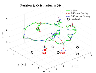
Figure 2: Vicon Room 2 01 experimental validation using a dataset. The true trajectories (green solid-line) and three axes true attitude (black solid-line) is plotted against the trajectory estimated by the proposed nonlinear stochastic discrete navigation observers (Algorithm 1; red dashed-line and blue center-line). The landmarks are plotted as black circles.

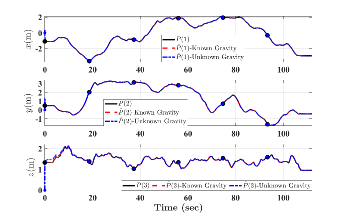
Figure 3: Position: true (black solid-line) vs estimated observers (red dashed-line and blue center-line).

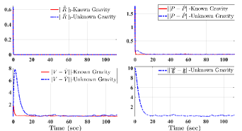
Figure 4: Error of proposed observers: Known Gravity vs Unknown Gravity.

V Conclusion

This paper addresses the problem of attitude, position, linear velocity, and gravity estimation of a vehicle traveling with 6 DoF. Nonlinear stochastic navigation observers on $\mathbb{SE}_{2}(3)$ has been proposed. The proposed observers are guaranteed to be almost SGUUB in the mean square. Experimental results revealed robustness and fast adaptability of the proposed approach for identification of unknown pose, linear velocity and gravity.

References

- [1] H. A. Hashim, “Systematic convergence of nonlinear stochastic estimators on the special orthogonal group SO(3),” International Journal of Robust and Nonlinear Control, vol. 30, no. 10, pp. 3848–3870, 2020.
- [2] J. L. Crassidis and F. L. Markley, “Unscented filtering for spacecraft attitude estimation,” Journal of guidance, control, and dynamics, vol. 26, no. 4, pp. 536–542, 2003.
- [3] H. F. Grip, T. I. Fossen, T. A. Johansen, and A. Saberi, “Attitude estimation using biased gyro and vector measurements with time-varying reference vectors,” IEEE Transactions on Automatic Control, vol. 57, no. 5, pp. 1332–1338, 2012.
- [4] H. A. Hashim, L. J. Brown, and K. McIsaac, “Nonlinear stochastic attitude filters on the special orthogonal group 3: Ito and stratonovich,” IEEE Transactions on Systems, Man, and Cybernetics: Systems, vol. 49, no. 9, pp. 1853–1865, 2019.
- [5] T. Lee, “Exponential stability of an attitude tracking control system on so (3) for large-angle rotational maneuvers,” Systems & Control Letters, vol. 61, no. 1, pp. 231–237, 2012.
- [6] H. A. Hashim, L. J. Brown, and K. McIsaac, “Nonlinear pose filters on the special euclidean group SE(3) with guaranteed transient and steady-state performance,” IEEE Transactions on Systems, Man, and Cybernetics: Systems, vol. PP, no. PP, pp. 1–14, 2019.
- [7] J. F. Vasconcelos, R. Cunha, C. Silvestre, and P. Oliveira, “A nonlinear position and attitude observer on se (3) using landmark measurements,” Systems & Control Letters, vol. 59, no. 3-4, pp. 155–166, 2010.
- [8] H. A. Hashim and F. L. Lewis, “Nonlinear stochastic estimators on the special euclidean group SE(3) using uncertain imu and vision measurements,” IEEE Transactions on Systems, Man, and Cybernetics: Systems, vol. PP, no. PP, pp. 1–14, 2020.
- [9] H. A. Hashim, “Guaranteed performance nonlinear observer for simultaneous localization and mapping,” IEEE Control Systems Letters, vol. 5, no. 1, pp. 91–96, 2021.
- [10] H. A. Hashim and A. E. E. Eltoukhy, “Landmark and imu data fusion: Systematic convergence geometric nonlinear observer for slam and velocity bias,” IEEE Transactions on Intelligent Transportation Systems, vol. PP, no. PP, pp. 1–10, 2020.
- [11] P. Batista, C. Silvestre, and P. Oliveira, “On the observability of linear motion quantities in navigation systems,” Systems & Control Letters, vol. 60, no. 2, pp. 101–110, 2011.
- [12] M.-D. Hua and G. Allibert, “Riccati observer design for pose, linear velocity and gravity direction estimation using landmark position and imu measurements,” in 2018 IEEE Conference on Control Technology and Applications (CCTA). IEEE, 2018, pp. 1313–1318.
- [13] A. Barrau and S. Bonnabel, “The invariant extended kalman filter as a stable observer,” IEEE Transactions on Automatic Control, vol. 62, no. 4, pp. 1797–1812, 2016.
- [14] H. Deng, M. Krstic, and R. J. Williams, “Stabilization of stochastic nonlinear systems driven by noise of unknown covariance,” IEEE Transactions on Automatic Control, vol. 46, no. 8, pp. 1237–1253, 2001.
- [15] K. Ito and K. M. Rao, Lectures on stochastic processes. Tata institute of fundamental research, 1984, vol. 24.
- [16] H. A. Hashim, “A geometric nonlinear stochastic filter for simultaneous localization and mapping,” Aerospace Science and Technology, vol. 111, p. 106569, 2021.
- [17] H.-B. Ji and H.-S. Xi, “Adaptive output-feedback tracking of stochastic nonlinear systems,” IEEE Transactions on Automatic Control, vol. 51, no. 2, pp. 355–360, 2006.
- [18] F. Bullo and A. D. Lewis, Geometric control of mechanical systems: modeling, analysis, and design for simple mechanical control systems. Springer Science & Business Media, 2004, vol. 49.
- [19] M. Burri, J. Nikolic, P. Gohl, T. Schneider, J. Rehder, S. Omari, M. W. Achtelik, and R. Siegwart, “The EuRoC micro aerial vehicle datasets,” The International Journal of Robotics Research, vol. 35, no. 10, pp. 1157–1163, 2016.
- [20] H. A. Hashim, “Special orthogonal group SO(3), euler angles, angle-axis, rodriguez vector and unit-quaternion: Overview, mapping and challenges,” arXiv preprint arXiv:1909.06669, 2019.